4/8: Cost Propagation & Partialization

Today’s lesson:Beware of solicitous suggestions from juvenile cosmetologists

Exhibit A: Abe LincolnExhibit B: Rao

Next Class: LPG—ICAPS 2003 paper. *READ* it before coming. Homework on SAPA coming from Vietnam

Multi-objective search

Multi-dimensional nature of plan quality in metric temporal planning: Temporal quality (e.g. makespan, slack) Plan cost (e.g. cumulative action cost, resource consumption)

Necessitates multi-objective optimization: Modeling objective functions Tracking different quality metrics and heuristic estimation Challenge: There may be inter-dependent

relations between different quality metric

Example

Option 1: Tempe Phoenix (Bus) Los Angeles (Airplane) Less time: 3 hours; More expensive: $200

Option 2: Tempe Los Angeles (Car) More time: 12 hours; Less expensive: $50

Given a deadline constraint (6 hours) Only option 1 is viable Given a money constraint ($100) Only option 2 is viable

Tempe

Phoenix

Los Angeles

Solution Quality in the presence of multiple objectives

When we have multiple objectives, it is not clear how to define global optimum

E.g. How does <cost:5,Makespan:7> plan compare to <cost:4,Makespan:9>? Problem: We don’t know what the user’s utility metric

is as a function of cost and makespan.

Solution 1: Pareto Sets

Present pareto sets/curves to the user A pareto set is a set of non-dominated solutions

A solution S1 is dominated by another S2, if S1 is worse than S2 in at least one objective and equal in all or worse in all other objectives. E.g. <C:4,M9> dominated by <C:5;M:9>

A travel agent shouldn’t bother asking whether I would like a flight that starts at 6pm and reaches at 9pm, and cost 100$ or another ones which also leaves at 6 and reaches at 9, but costs 200$.

A pareto set is exhaustive if it contains all non-dominated solutions Presenting the pareto set allows the users to state their preferences implicitly by

choosing what they like rather than by stating them explicitly. Problem: Exhaustive Pareto sets can be large (non-finite in many cases).

In practice, travel agents give you non-exhaustive pareto sets, just so you have the illusion of choice

Optimizing with pareto sets changes the nature of the problem—you are looking for multiple rather than a single solution.

Solution 2: Aggregate Utility Metrics

Combine the various objectives into a single utility measure Eg: w1*cost+w2*make-span

Could model grad students’ preferences; with w1=infinity, w2=0 Log(cost)+ 5*(Make-span)25

Could model Bill Gates’ preferences. How do we assess the form of the utility measure (linear? Nonlinear?) and how will we get the weights?

Utility elicitation process Learning problem: Ask tons of questions to the users and learn their utility function to fit their preferences

Can be cast as a sort of learning task (e.g. learn a neual net that is consistent with the examples) Of course, if you want to learn a true nonlinear preference function, you will need many many more examples, and the

training takes much longer.

With aggregate utility metrics, the multi-obj optimization is, in theory, reduces to a single objective optimization problem *However* if you are trying to good heuristics to direct the search, then since estimators are likely to be

available for naturally occurring factors of the solution quality, rather than random combinations there-of, we still have to follow a two step process

1. Find estimators for each of the factors2. Combine the estimates using the utility measure THIS IS WHAT WE WILL DO IN THE NEXT FEW SLIDES

Our approach

Using the Temporal Planning Graph (Smith & Weld) structure to track the time-sensitive cost function: Estimation of the earliest time (makespan) to achieve all goals. Estimation of the lowest cost to achieve goals Estimation of the cost to achieve goals given the specific

makespan value. Using this information to calculate the heuristic

value for the objective function involving both time and cost

New issue: How to propagate cost over planning graphs?

The (Relaxed) Temporal PG

Tempe

Phoenix

Los Angeles

Drive-car(Tempe,LA)

Heli(T,P)

Shuttle(T,P)

Airplane(P,LA)

t = 0 t = 0.5 t = 1 t = 1.5 t = 10

Time-sensitive Cost Function

Standard (Temporal) planning graph (TPG) shows the time-related estimates e.g. earliest time to achieve fact, or to execute action

TPG does not show the cost estimates to achieve facts or execute actions

Tempe

Phoenix

L.A

Shuttle(Tempe,Phx): Cost: $20; Time: 1.0 hourHelicopter(Tempe,Phx):Cost: $100; Time: 0.5 hourCar(Tempe,LA):Cost: $100; Time: 10 hourAirplane(Phx,LA):Cost: $200; Time: 1.0 hour

cost

time0 1.5 2 10

$300

$220

$100

Drive-car(Tempe,LA)

Heli(T,P)

Shuttle(T,P)

Airplane(P,LA)

t = 0 t = 0.5 t = 1 t = 1.5 t = 10

Estimating the Cost Function

Tempe

Phoenix

L.A

time0 1.5 2 10

$300

$220

$100

t = 1.5 t = 10

Shuttle(Tempe,Phx): Cost: $20; Time: 1.0 hourHelicopter(Tempe,Phx):Cost: $100; Time: 0.5 hourCar(Tempe,LA):Cost: $100; Time: 10 hourAirplane(Phx,LA):Cost: $200; Time: 1.0 hour

1

Drive-car(Tempe,LA)

Hel(T,P)

Shuttle(T,P)

t = 0

Airplane(P,LA)

t = 0.5

0.5

t = 1

Cost(At(LA)) Cost(At(Phx)) = Cost(Flight(Phx,LA))

Airplane(P,LA)

t = 2.0

$20

Cost Propagation Issues:

At a given time point, each fact is supported by multiple actions Each action has more than one precondition

Propagation rules: Cost(f,t) = min {Cost(A,t) : f Effect(A)} Cost(A,t) = Aggregate(Cost(f,t): f Pre(A))

Sum-propagation: Cost(f,t) The plans for individual preconds may be interacting

Max-propagation: Max {Cost(f,t)} Combination: 0.5 Cost(f,t) + 0.5 Max {Cost(f,t)}

Probably other better ideas could be tried

Can’t use something like set-level idea here becauseThat will entail tracking the costs of subsets of literals

Termination Criteria

Deadline Termination: Terminate at time point t if: goal G: Dealine(G) t goal G: (Dealine(G) < t) (Cost(G,t) =

Fix-point Termination: Terminate at time point t where we can not improve the cost of any proposition.

K-lookahead approximation: At t where Cost(g,t) < , repeat the process of applying (set) of actions that can improve the cost functions k times.

cost

time0 1.5 2 10

$300

$220

$100

Drive-car(Tempe,LA)

H(T,P)

Shuttle(T,P)

Plane(P,LA)

t = 0 0.5 1 1.5 t = 10

Earliest time pointCheapest cost

Heuristic estimation using the cost functions

If the objective function is to minimize time: h = t0

If the objective function is to minimize cost: h = CostAggregate(G, t)

If the objective function is the function of both time and cost

O = f(time,cost) then:h = min f(t,Cost(G,t)) s.t. t0 t t

Eg: f(time,cost) = 100.makespan + Cost then h = 100x2 + 220 at t0 t = 2 t

time

cost

0 t0=1.5 2 t = 10

$300

$220

$100

Cost(At(LA))

Earliest achieve time: t0 = 1.5Lowest cost time: t = 10

The cost functions have information to track both temporal and costmetric of the plan, and their inter-dependent relations !!!

Heuristic estimation by extracting the relaxed plan

Relaxed plan satisfies all the goals ignoring the negative interaction: Take into account positive interaction Base set of actions for possible adjustment according to

neglected (relaxed) information (e.g. negative interaction, resource usage etc.)

Need to find a good relaxed plan (among multiple ones) according to the objective function

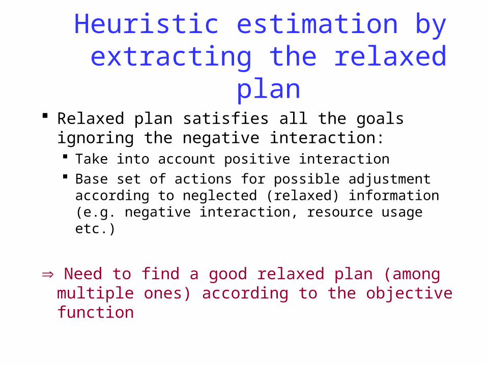
Heuristic estimation by extracting the relaxed plan

General Alg.: Traverse backward searching for actions supporting all the goals. When A is added to the relaxed plan RP, then:

Supported Fact = SF Effects(A)Goals = SF \ (G Precond(A))

Temporal Planning with Cost: If the objective function is f(time,cost), then A is selected such that:

f(t(RP+A),C(RP+A)) + f(t(Gnew),C(Gnew)) is minimal (Gnew = (G Precond(A)) \ Effects)

Finally, using mutex to set orders between A and actions in RP so that less number of causal constraints are violated

time

cost

0 t0=1.5 2 t = 10

$300

$220

$100

Tempe

Phoenix

L.A

f(t,c) = 100.makespan + Cost

Adjusting the Heuristic Values

Ignored resource related information can be used to improve the heuristic values (such like +ve and –ve interactions in classical planning)

Adjusted Cost:

C = C + R (Con(R) – (Init(R)+Pro(R)))/R * C(AR)

Cannot be applied to admissible heuristics

4/10

Partialization Example

A1 A2 A3

A1(10) gives g1 but deletes pA3(8) gives g2 but requires p at startA2(4) gives p at end We want g1,g2

A position-constrained plan with makespan 22

A1

A2

A3 G

p

g1

g2

[et(A1) <= et(A2)] or [st(A1) >= st(A3)][et(A2) <= st(A3)….

OrderConstrainedplan

The best makespan dispatch of the order-constrained plan

A1

A2 A3 14+

There could be multiple O.C. plansbecause of multiple possible causal sources. Optimization will involve Going through them all.

Problem Definitions Position constrained (p.c) plan: The execution time of each action is

fixed to a specific time point Can be generated more efficiently by state-space planners

Order constrained (o.c) plan: Only the relative orderings between actions are specified More flexible solutions, causal relations between actions

Partialization: Constructing a o.c plan from a p.c plan

QR R

G

QR

{Q} {G}

t1 t2 t3

p.c plan o.c plan

Q R RG

QR

{Q} {G}

Validity Requirements for a partialization

An o.c plan Poc is a valid partialization of a valid p.c plan Ppc, if: Poc contains the same actions as Ppc

Poc is executable Poc satisfies all the top level goals (Optional) Ppc is a legal dispatch (execution) of Poc

(Optional) Contains no redundant ordering relations

PQ

PQ

Xredundant

Greedy Approximations

Solving the optimization problem for makespan and number of orderings is NP-hard (Backstrom,1998)

Greedy approaches have been considered in classical planning (e.g. [Kambhampati & Kedar, 1993], [Veloso et. al.,1990]):

Find a causal explanation of correctness for the p.c plan Introduce just the orderings needed for the explanation to

hold

Modeling greedy approaches as value ordering strategies

Variation of [Kambhampati & Kedar,1993] greedy algorithm for temporal planning as value ordering: Supporting variables: Sp

A = A’ such that: etp

A’ < stpA in the p.c plan Ppc

B s.t.: etpA’ < etp

B < stpA

C s.t.: etpC < etp

A’ and satisfy two above conditions Ordering and interference variables:

pAB = < if etp

B < stpA ; p

AB = > if stpB > stp

A

rAA’= < if etr

A < strA’ in Ppc; r

AA’= > if strA > etr

A’ in Ppc; rAA’= other wise.

Key insight: We can capture many of the greedy approaches as specific value ordering strategies on the CSOP encoding

Empirical evaluation

Objective: Demonstrate that metric temporal planner armed with our

approach is able to produce plans that satisfy a variety of cost/makespan tradeoff.

Testing problems: Randomly generated logistics problems from TP4

(Hasslum&Geffner)Load/unload(package,location): Cost = 1; Duration = 1;Drive-inter-city(location1,location2): Cost = 4.0; Duration = 12.0;Flight(airport1,airport2): Cost = 15.0; Duration = 3.0;Drive-intra-city(location1,location2,city): Cost = 2.0; Duration = 2.0;

LPG Discussion—Look at notes of Week 12 (as they are more uptodate)