4D Seismic Interpretation of the Norne Field - A … Semi-quantitative Approach ... This paper shows a workflow for the 4D seismic interpretation of the Norne field ... The interpretation

30 May – 2 June 2016 | Reed Messe Wien

78th EAGE Conference & Exhibition 2016 Vienna, Austria, 30 May – 2 June 2016

Th LHR2 024D Seismic Interpretation of the Norne Field - ASemi-quantitative ApproachJ.M.C. Santos* (University of Campinas), A. Davolio (University ofCampinas), C. MacBeth (Heriot-Watt University) & D.J. Schiozer (Universityof Campinas)

SUMMARYThis paper shows a workflow for the 4D seismic interpretation of the Norne field benchmark case and theuse to better understand how 4D seismic data can be input for updating the simulation model. Theinterpretation was performed in two passes. The first pass aimed to understand the character of the seismicdata, identify the anomalies in the data and how they relate to the well activities and fluid movement in thefield. The second pass consisted of integrating this previous seismic understanding into the simulationdata, distinguishing pressure and saturation effects and recognizing how they relate to the rock physicsand/or the static and dynamic parameters from the simulation model. Simulation to seismic (sim2seis)was performed to relate the simulation response to the seismic domain. We show several examples ofinconsistencies between the sim2seis predicted response and the observed seismic data, and evaluatewhether these are caused by a simulation model inaccuracy or by uncertainties in the actual seismicresponse. After this careful qualitative and semi-quantitative analysis, we ranked the data we are mostconfident in before implementing the desired updates.



Introduction

4D seismic is an important reservoir management tool and often used in the simulation model updating process. However, an important aspect is the information provided by 4D seismic at the history matching process, which must reflect a good understanding of the character of the seismic and its interpretation. For this reason, we propose a workflow that aims to first evaluate the areas where the simulation model properties should be adjusted and second to identify the areas where 4D seismic data information can be confidently incorporated for adjusting the simulation model. We show examples of inconsistencies between the seismic response predicted from the simulation model and the observed seismic for the Norne field benchmark case. These inconsistencies are then investigated in more detail, evaluating whether they are caused by a simulation model inaccuracy or by uncertainties in the actual seismic response.

Calibration and updating workflow

The interpretation of the 4D seismic data was done in two passes, with the level of quantitativeness increasing throughout the study. The first pass aimed to understand the character of the seismic, identify the anomalies in the data and how they relate to the well activities and fluid movement from the field. The second pass integrated this seismic understanding with the simulation data, distinguishing pressure and saturation effects and recognizing how they relate to the rock physics, and to the static and dynamic parameters from the simulation model. Simulation to seismic (sim2seis) was performed to bring the simulation response to the seismic domain. Next, a search for mismatches between sim2seis synthetic and actual seismic response is considered. Lastly, we assess the possible causes for the mismatch, and if this information can be incorporated for improving the simulation model. A rank of the data which we are most confident in is also a tool we will use before fully implementing the simulation model updates.

Data examples

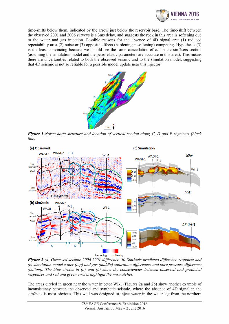
Our methodology was applied in the Norne field benchmark case made available by Statoil and license partners. The Norne field is a 3x 9km horst structure located in the Norwegian Sea. It consists of two separate oil compartments, the Norne Main Structure (C, D and E-segments), containing 97% of the oil in place, and the Northeast Segment (G-segment). A gas filled soft sandstone (Garn Formation) and the gas oil contact in the vicinity of the Not Formation claystones were discovered in 1991 and production started in 1997 (Statoil 2004). The seismic surveys acquired in 2001, 2003, 2004 and 2006 were available for this study. Four areas from the field were selected as examples, one in each segment. The first example is from a vertical section extracted along the C, D and E segments, represented by the black line in Figure 1. This section crosses the location of two WAG injectors (WAG-1 and 2) which have been operating since 1998, one oil/gas producer (P-1), open in the end of 1997, and one water injector (WI-1), operating since 1999 at the north of E-segment. Figure 2a shows the 2006 minus 2001 4D difference of the observed seismic data, Figure 2b shows the same 4D difference from sim2seis and Figures 2c show the simulated differences for the same time-steps. In Figures 2a and 2b we firstly note a weak 4D response picked at the top reservoir, this was expected as all changes are occurring at a deeper level. The anomalies are laterally contained by the faults in grey. We note a reasonable match between the water saturation increase anomaly (hardening effect) from the sim2seis and the observed seismic in the D-segment (blue circles from Figures 2a and 2b). However, there are big mismatches near WAG-1 and WI-1 wells (red and green circles respectively, from Figures 2a and 2b). The WAG-1 area shows the sim2seis anomaly (red circles from Figures 2a and 2b) which could be both softening (increase of gas saturation and pressure build up response) or a hardening (water saturation increase) response. This anomaly is not seen on the observed data, however, we see the



time-shifts below them, indicated by the arrow just below the reservoir base. The time-shift between the observed 2001 and 2006 surveys is a 3ms delay, and suggests the rock in this area is softening due to the water and gas injection. Possible reasons for the absence of 4D signal are: (1) reduced repeatability area (2) noise or (3) opposite effects (hardening + softening) competing. Hypothesis (3) is the least convincing because we should see the same cancellation effect in the sim2seis section (assuming the simulation model and the petro-elastic parameters are accurate in this area). This means there are uncertainties related to both the observed seismic and to the simulation model, suggesting that 4D seismic is not so reliable for a possible model update near this injector.

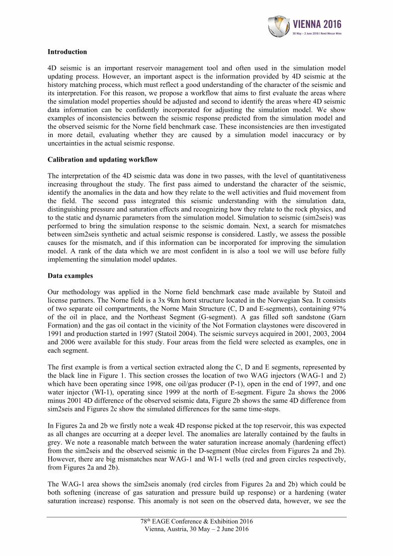
Figure 1 Norne horst structure and location of vertical section along C, D and E segments (black line).

Figure 2 (a) Observed seismic 2006-2001 difference (b) Sim2seis predicted difference response and (c) simulation model water (top) and gas (middle) saturation differences and pore pressure difference (bottom). The blue circles in (a) and (b) show the consistencies between observed and predicted responses and red and green circles highlight the mismatches. The areas circled in green near the water injector WI-1 (Figures 2a and 2b) show another example of inconsistency between the observed and synthetic seismic, where the absence of 4D signal in the sim2seis is most obvious. This well was designed to inject water in the water leg from the northern

Time‐shifts



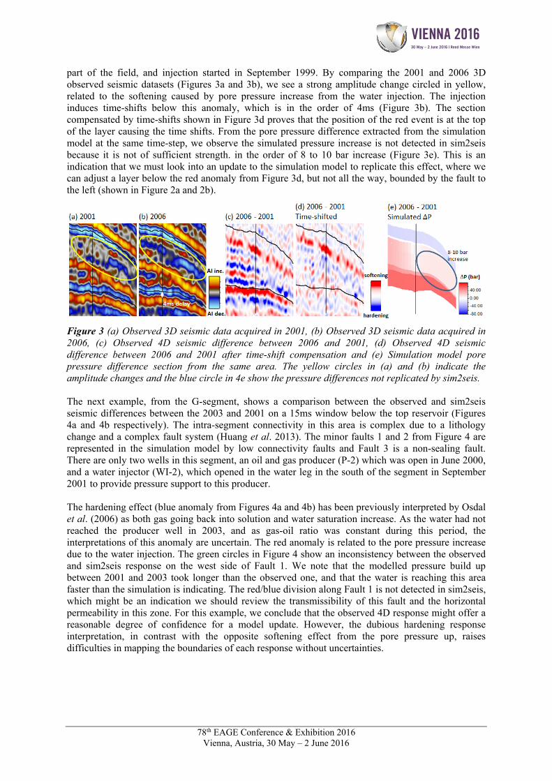
part of the field, and injection started in September 1999. By comparing the 2001 and 2006 3D observed seismic datasets (Figures 3a and 3b), we see a strong amplitude change circled in yellow, related to the softening caused by pore pressure increase from the water injection. The injection induces time-shifts below this anomaly, which is in the order of 4ms (Figure 3b). The section compensated by time-shifts shown in Figure 3d proves that the position of the red event is at the top of the layer causing the time shifts. From the pore pressure difference extracted from the simulation model at the same time-step, we observe the simulated pressure increase is not detected in sim2seis because it is not of sufficient strength. in the order of 8 to 10 bar increase (Figure 3e). This is an indication that we must look into an update to the simulation model to replicate this effect, where we can adjust a layer below the red anomaly from Figure 3d, but not all the way, bounded by the fault to the left (shown in Figure 2a and 2b).

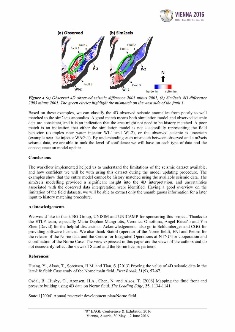
Figure 3 (a) Observed 3D seismic data acquired in 2001, (b) Observed 3D seismic data acquired in 2006, (c) Observed 4D seismic difference between 2006 and 2001, (d) Observed 4D seismic difference between 2006 and 2001 after time-shift compensation and (e) Simulation model pore pressure difference section from the same area. The yellow circles in (a) and (b) indicate the amplitude changes and the blue circle in 4e show the pressure differences not replicated by sim2seis. The next example, from the G-segment, shows a comparison between the observed and sim2seis seismic differences between the 2003 and 2001 on a 15ms window below the top reservoir (Figures 4a and 4b respectively). The intra-segment connectivity in this area is complex due to a lithology change and a complex fault system (Huang et al. 2013). The minor faults 1 and 2 from Figure 4 are represented in the simulation model by low connectivity faults and Fault 3 is a non-sealing fault. There are only two wells in this segment, an oil and gas producer (P-2) which was open in June 2000, and a water injector (WI-2), which opened in the water leg in the south of the segment in September 2001 to provide pressure support to this producer. The hardening effect (blue anomaly from Figures 4a and 4b) has been previously interpreted by Osdal et al. (2006) as both gas going back into solution and water saturation increase. As the water had not reached the producer well in 2003, and as gas-oil ratio was constant during this period, the interpretations of this anomaly are uncertain. The red anomaly is related to the pore pressure increase due to the water injection. The green circles in Figure 4 show an inconsistency between the observed and sim2seis response on the west side of Fault 1. We note that the modelled pressure build up between 2001 and 2003 took longer than the observed one, and that the water is reaching this area faster than the simulation is indicating. The red/blue division along Fault 1 is not detected in sim2seis, which might be an indication we should review the transmissibility of this fault and the horizontal permeability in this zone. For this example, we conclude that the observed 4D response might offer a reasonable degree of confidence for a model update. However, the dubious hardening response interpretation, in contrast with the opposite softening effect from the pore pressure up, raises difficulties in mapping the boundaries of each response without uncertainties.



Figure 4 (a) Observed 4D observed seismic difference 2003 minus 2001, (b) Sim2seis 4D difference 2003 minus 2001. The green circles highlight the mismatch on the west side of the fault 1. Based on these examples, we can classify the 4D observed seismic anomalies from poorly to well matched to the sim2seis anomalies. A good match means both simulation model and observed seismic data are consistent, and it is an indication that the area might not need to be history matched. A poor match is an indication that either the simulation model is not successfully representing the field behavior (examples near water injector WI-1 and WI-2), or the observed seismic is uncertain (example near the injector WAG-1). By understanding each mismatch between observed and sim2seis seismic data, we are able to rank the level of confidence we will have on each type of data and the consequence on model update.

Conclusions

The workflow implemented helped us to understand the limitations of the seismic dataset available, and how confident we will be with using this dataset during the model updating procedure. The examples show that the entire model cannot be history matched using the available seismic data. The sim2seis modelling provided a significant insight into the 4D interpretation, and uncertainties associated with the observed data interpretation were identified. Having a good overview on the limitation of the field datasets, we will be able to extract only the unambiguous information for a later input to history matching procedure.

Acknowledgements

We would like to thank BG Group, UNISIM and UNICAMP for sponsoring this project. Thanks to the ETLP team, especially Maria-Daphne Mangriotis, Veronica Omofoma, Angel Briceño and Yin Zhen (David) for the helpful discussions. Acknowledgements also go to Schlumberger and CGG for providing software licences. We also thank Statoil (operator of the Norne field), ENI and Petoro for the release of the Norne data and the Centre for Integrated Operations at NTNU for cooperation and coordination of the Norne Case. The view expressed in this paper are the views of the authors and do not necessarily reflect the views of Statoil and the Norne license partners.

References

Huang, Y., Alsos, T., Sorensen, H.M. and Tian, S. [2013] Proving the value of 4D seismic data in the late-life field: Case study of the Norne main field. First Break, 31(9), 57-67. Osdal, B., Husby, O., Aronsen, H.A., Chen, N. and Alsos, T. [2006] Mapping the fluid front and pressure buildup using 4D data on Norne field. The Leading Edge, 25, 1134-1141. Statoil [2004] Annual reservoir development plan/Norne field.

Documents

4D Seismic Interpretation of the Norne Field - A … Semi-quantitative Approach ... This paper shows a workflow for the 4D seismic interpretation of the Norne field ... The interpretation