5. Chapter 5 Vibroseis- A Very Special Source

Chapter 5 Vibroseis: A Very Special Source

In conclusion, it should be said that the critical comments made in this paper were made out of concerned admiration for the Vibroseis technique. It should not be forgotten that, apart from its success as an exploration tool, it has stimu-lated more interest and contributed more to our understanding of seismology than any other technique. The vibrator remains the most sophisticated energy source with the greatest possibilities for development.

—W. E. Lerwill (Lerwill, 1981, p. 526)

Introduction

The vibroseis method was introduced in the mid-1950s by Conoco. The name Vibroseis was a trademark of Continental Oil Company, granted in 1962. William Doty and John Crawford applied for the original patent on 27 February 1953, and it was granted on 31 August 1954. The first claim of this patent is as follows (Doty and Craw-ford, 1954, p. 7):

Broadly stated, the present invention comprises a method of determining the travel time, between spaced first and second points, of a unique signal having vibration energy which is non-repetitive during a period which is at least as long as such travel time, comprising

(a) Transmitting such a signal from said first point,(b) Providing a counterpart of said transmitted signal,(c) Multiplying

(i) at least a substantial portion of the total transmitted vibration energy of said signal which is received at said second point, by

(ii) said counterpart signal,(d) Integrating for a substantial period the product of said multiplication,

and altering the phase relation between said counterpart signal and said transmitted signal during successive integrating periods, and

(e) Recording the values derived from such integration; whereby the out-of-time-phase relation of said counterpart signal with respect to the transmitted signal at said first point, which yields the greatest value from such integration, may be used as a parameter of the travel time of said unique signal between said points.

Distinguished Instructor Short Course • 97

Dow

nloa

ded

01/1

7/13

to 1

92.1

59.1

06.2

00. R

edis

trib

utio

n su

bjec

t to

SEG

lice

nse

or c

opyr

ight

; see

Ter

ms

of U

se a

t http

://lib

rary

.seg

.org

/

In 1953, the seismic business focused mainly on measuring traveltimes, which still are the center of our attention. Perhaps we can obtain slightly better precision now, and after almost 60 years, we can measure more than just traveltimes.

Doty and Crawford (1954) include a description of correlation, but surprisingly, they never use the word correlation itself. Could we describe vibroseis operations without using that word today?

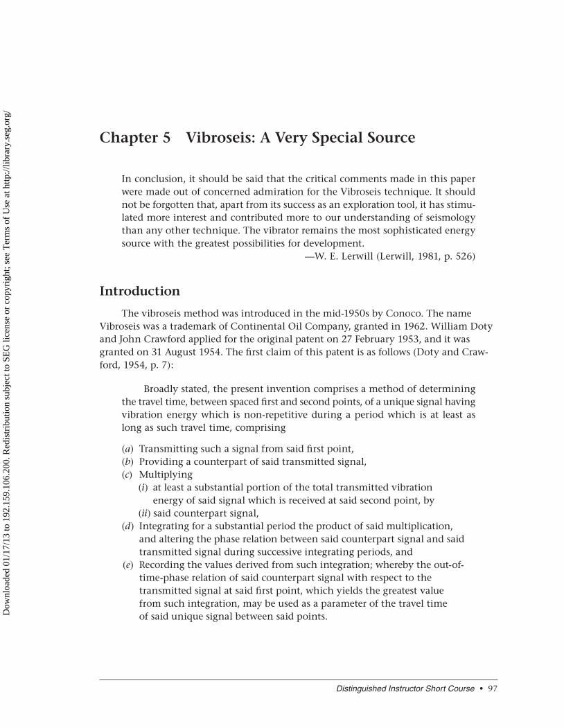
The vibrator started life as an alternative to explosive sources on land. It had to com-pete for a short time with weight-drop trucks, but they could not be synchronized, whereas vibrators could. After various technologies were tested (Figure 1), hydraulic technology was

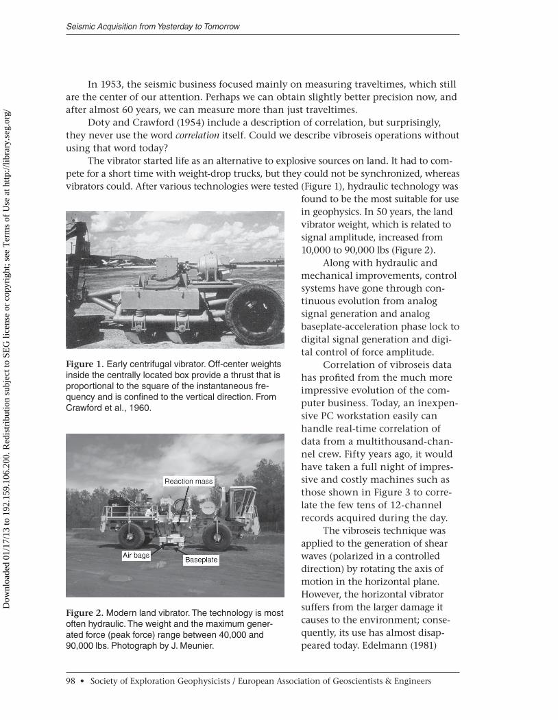
found to be the most suitable for use in geophysics. In 50 years, the land vibrator weight, which is related to signal amplitude, increased from 10,000 to 90,000 lbs (Figure 2).

Along with hydraulic and mechanical improvements, control systems have gone through con-tinuous evolution from analog signal generation and analog baseplate-acceleration phase lock to digital signal generation and digi-tal control of force amplitude.

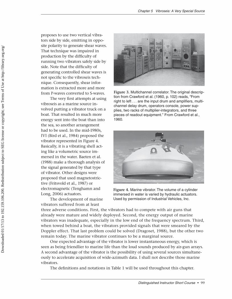
Correlation of vibroseis data has profited from the much more impressive evolution of the com-puter business. Today, an inexpen-sive PC workstation easily can handle real-time correlation of data from a multithousand-chan-nel crew. Fifty years ago, it would have taken a full night of impres-sive and costly machines such as those shown in Figure 3 to corre-late the few tens of 12-channel records acquired during the day.

The vibroseis technique was applied to the generation of shear waves (polarized in a controlled direction) by rotating the axis of motion in the horizontal plane. However, the horizontal vibrator suffers from the larger damage it causes to the environment; conse-quently, its use has almost disap-peared today. Edelmann (1981)

Seismic Acquisition from Yesterday to Tomorrow

98 • Society of Exploration Geophysicists / European Association of Geoscientists & Engineers

Figure 1. Early centrifugal vibrator. Off-center weights inside the centrally located box provide a thrust that is proportional to the square of the instantaneous fre-quency and is confined to the vertical direction. From Crawford et al., 1960.

Figure 2. Modern land vibrator. The technology is most often hydraulic. The weight and the maximum gener-ated force (peak force) range between 40,000 and 90,000 lbs. Photograph by J. Meunier.

Dow

nloa

ded

01/1

7/13

to 1

92.1

59.1

06.2

00. R

edis

trib

utio

n su

bjec

t to

SEG

lice

nse

or c

opyr

ight

; see

Ter

ms

of U

se a

t http

://lib

rary

.seg

.org

/

proposes to use two vertical vibra-tors side by side, emitting in oppo-site polarity to generate shear waves. That technique was impaired in production by the difficulty of running two vibrators safely side by side. Note that the difficulty of generating controlled shear waves is not specific to the vibroseis tech-nique. Consequently, shear infor-mation is extracted more and more from P-waves converted to S-waves.

The very first attempts at using vibroseis as a marine source in-volved putting a vibrator truck on a boat. That resulted in much more energy sent into the boat than into the sea, so another arrangement had to be used. In the mid-1980s, IVI (Bird et al., 1984) proposed the vibrator represented in Figure 4. Basically, it is a vibrating shell act-ing like a volumetric source im-mersed in the water. Baeten et al. (1988) make a thorough analysis of the signal generated by that type of vibrator. Other designs were proposed that used magnetostric-tive (Fritsvold et al., 1987) or electro magnetic (Tenghamn and Long, 2006) actuators.

The development of marine vibrators suffered from at least three adverse conditions. First, the vibrators had to compete with air guns that already were mature and widely deployed. Second, the energy output of marine vibrators was inadequate, especially in the low end of the frequency spectrum. Third, when towed behind a boat, the vibrators provided signals that were smeared by the Doppler effect. That last problem could be solved (Dragoset, 1988), but the other two remain today. The marine vibrator continues to be a marginal source.

One expected advantage of the vibrator is lower instantaneous energy, which is seen as being friendlier to marine life than the loud sounds produced by air-gun arrays. A second advantage of the vibrator is the possibility of using several sources simultane-ously to accelerate acquisition of wide-azimuth data. I shall not describe those marine vibrators.

The definitions and notations in Table 1 will be used throughout this chapter.



Figure 3. Multichannel correlator. The original descrip-tion from Crawford et al. (1960, p. 102) reads, “From right to left . . . are the input drum and amplifiers, multi-channel delay drum, operators console, power sup-plies, two racks of multiplier-integrators, and three pieces of readout equipment.” From Crawford et al., 1960.

Figure 4. Marine vibrator. The volume of a cylinder immersed in water is varied by hydraulic actuators. Used by permission of Industrial Vehicles, Inc.

Dow

nloa

ded

01/1

7/13

to 1

92.1

59.1

06.2

00. R

edis

trib

utio

n su

bjec

t to

SEG

lice

nse

or c

opyr

ight

; see

Ter

ms

of U

se a

t http

://lib

rary

.seg

.org

/

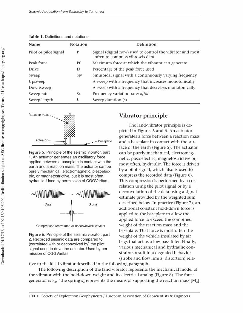
Vibrator principle

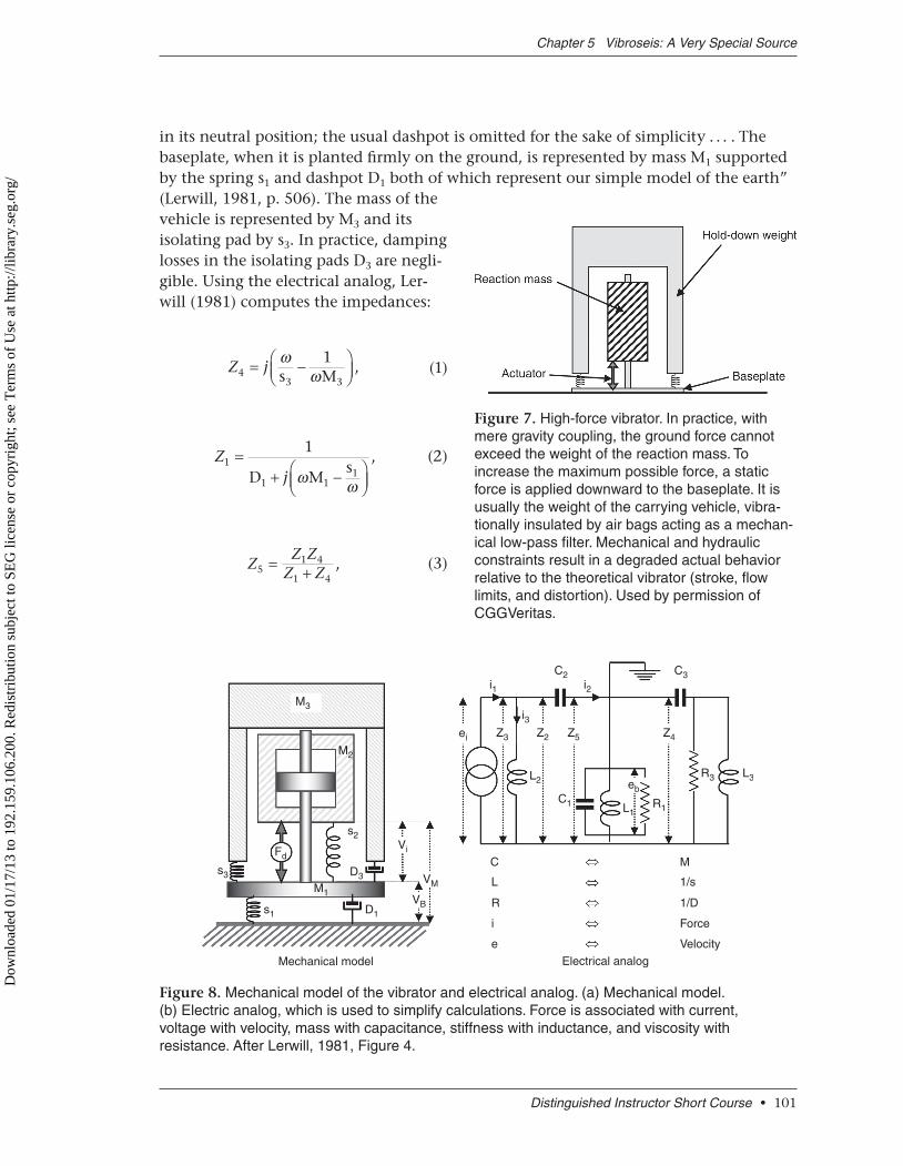
The land-vibrator principle is de-picted in Figures 5 and 6. An actuator generates a force between a reaction mass and a baseplate in contact with the sur-face of the earth (Figure 5). The actuator can be purely mechanical, electromag-netic, piezoelectric, magnetostrictive or, most often, hydraulic. The force is driven by a pilot signal, which also is used to compress the recorded data (Figure 6). This compression is performed by a cor-relation using the pilot signal or by a deconvolution of the data using a signal estimate provided by the weighted sum described below. In practice (Figure 7), an additional constant hold-down force is applied to the baseplate to allow the applied force to exceed the combined weight of the reaction mass and the baseplate. That force is most often the weight of the vehicle insulated by air bags that act as a low-pass filter. Finally, various mechanical and hydraulic con-straints result in a degraded behavior (stroke and flow limits, distortion) rela-

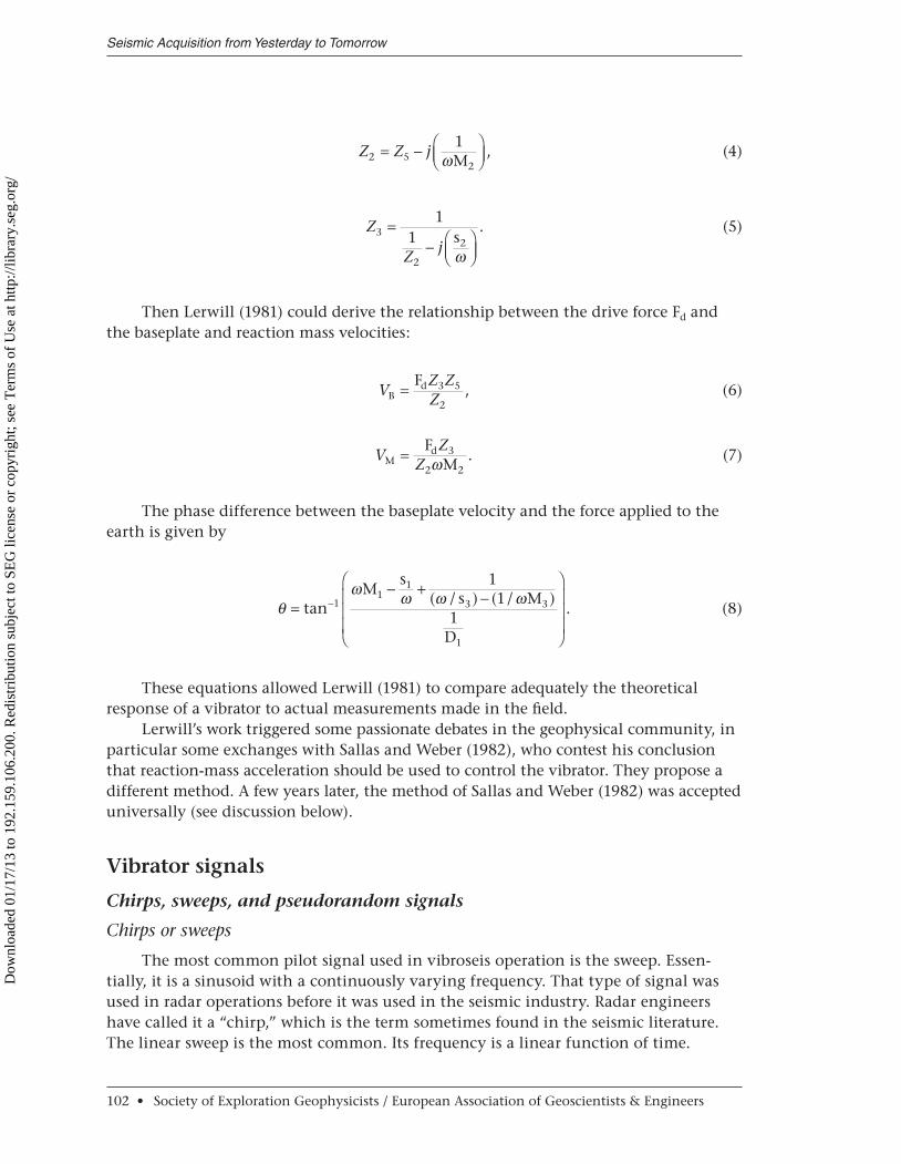
tive to the ideal vibrator described in the following paragraph.The following description of the land vibrator represents the mechanical model of

the vibrator with the hold-down weight and its electrical analog (Figure 8). The force generator is Fd, “the spring s2 represents the means of supporting the reaction mass [M2]



Figure 5. Principle of the seismic vibrator, part 1. An actuator generates an oscillatory force applied between a baseplate in contact with the earth and a reaction mass. The actuator can be purely mechanical, electromagnetic, piezoelec-tric, or magnetostrictive, but it is most often hydraulic. Used by permission of CGGVeritas.

Figure 6. Principle of the seismic vibrator, part 2. Re corded seismic data are compared to (correlated with or deconvolved by) the pilot signal used to drive the actuator. Used by per-mission of CGGVeritas.

Table 1. Definitions and notations.

Name Notation Definition

Pilot or pilot signal P Signal (digital now) used to control the vibrator and most often to compress vibroseis data

Peak force Pf Maximum force at which the vibrator can generate

Drive D Percentage of the peak force used

Sweep Sw Sinusoidal signal with a continuously varying frequency

Upsweep A sweep with a frequency that increases monotonically

Downsweep A sweep with a frequency that decreases monotonically

Sweep rate Sr Frequency variation rate: df/dt

Sweep length L Sweep duration (s)

Dow

nloa

ded

01/1

7/13

to 1

92.1

59.1

06.2

00. R

edis

trib

utio

n su

bjec

t to

SEG

lice

nse

or c

opyr

ight

; see

Ter

ms

of U

se a

t http

://lib

rary

.seg

.org

/

in its neutral position; the usual dashpot is omitted for the sake of simplicity . . . . The baseplate, when it is planted firmly on the ground, is represented by mass M1 supported by the spring s1 and dashpot D1 both of which represent our simple model of the earth” (Lerwill, 1981, p. 506). The mass of the vehicle is represented by M3 and its isolating pad by s3. In practice, damping losses in the isolating pads D3 are negli-gible. Using the electrical analog, Ler-will (1981) computes the impedances:

Z j4

3 3

1= -ÊËÁ

ˆ¯̃

wws M

,

(1)

Zj

1

1 11

1=+ -Ê

ËÁˆ¯̃

D Msw w

,

(2)

Z

Z ZZ Z5

1 4

1 4= + ,

(3)



Figure 7. High-force vibrator. In practice, with mere gravity coupling, the ground force cannot exceed the weight of the reaction mass. To increase the maximum possible force, a static force is applied downward to the baseplate. It is usually the weight of the carrying vehicle, vibra-tionally insulated by air bags acting as a mechan-ical low-pass filter. Mechanical and hydraulic constraints result in a degraded actual behavior relative to the theoretical vibrator (stroke, flow limits, and distortion). Used by permission of CGGVeritas.

Mechanical model

M3

M2

s2

s3

s1 D1

VB

Vi

ei Z3 Z2 Z5 Z4

L2

C1

C

L

R

i

e

M

1/s

1/D

Force

Velocity

Electrical analog

eb

L1R1

i3

i1 i2

C2

R3 L3

C3

VMM1

Fd

D3

Figure 8. Mechanical model of the vibrator and electrical analog. (a) Mechanical model. (b) Electric analog, which is used to simplify calculations. Force is associated with current, voltage with velocity, mass with capacitance, stiffness with inductance, and viscosity with resistance. After Lerwill, 1981, Figure 4.

Dow

nloa

ded

01/1

7/13

to 1

92.1

59.1

06.2

00. R

edis

trib

utio

n su

bjec

t to

SEG

lice

nse

or c

opyr

ight

; see

Ter

ms

of U

se a

t http

://lib

rary

.seg

.org

/

Z Z j2 5

2

1= - ÊËÁ

ˆ¯̃wM

,

(4)

Z

Zj

3

2

2

11

=- Ê

ËÁˆ¯̃

sw

.

(5)

Then Lerwill (1981) could derive the relationship between the drive force Fd and the baseplate and reaction mass velocities:

V

Z ZZB

dF= 3 5

2,

(6)

V

ZZM

dFM

= 3

2 2w .

(7)

The phase difference between the baseplate velocity and the force applied to the earth is given by

qw w w w=

- + -Ê

Ë

ÁÁÁ

ˆ

¯

˜˜˜

-tan( / ) ( / )

.11

1

3 3

1

11

1

Ms

s M

D

(8)

These equations allowed Lerwill (1981) to compare adequately the theoretical response of a vibrator to actual measurements made in the field.

Lerwill’s work triggered some passionate debates in the geophysical community, in particular some exchanges with Sallas and Weber (1982), who contest his conclusion that reaction-mass acceleration should be used to control the vibrator. They propose a different method. A few years later, the method of Sallas and Weber (1982) was accepted universally (see discussion below).

Vibrator signals

Chirps, sweeps, and pseudorandom signals

Chirps or sweeps

The most common pilot signal used in vibroseis operation is the sweep. Essen-tially, it is a sinusoid with a continuously varying frequency. That type of signal was used in radar operations before it was used in the seismic industry. Radar engineers have called it a “chirp,” which is the term sometimes found in the seismic literature. The linear sweep is the most common. Its frequency is a linear function of time.



Dow

nloa

ded

01/1

7/13

to 1

92.1

59.1

06.2

00. R

edis

trib

utio

n su

bjec

t to

SEG

lice

nse

or c

opyr

ight

; see

Ter

ms

of U

se a

t http

://lib

rary

.seg

.org

/

For a linear sweep, if t represents time, L is the sweep duration, and f is frequency, starting at f = f1 for t = 0 and ending at f = f2 for t = L, then

f f f f

tL

= + -( )1 2 1 .

(9)

The frequency in Hertz is the derivative of the phase (normalized by 2π), and thus the phase is given by

f p f= + -( )Ê

ËÁˆ¯̃

+221 2 1

2

0f t f ftL

,

(10)

where φ0 is the phase at time t = 0.If a0 is the peak amplitude, the sweep is given by

S t a f t f f

tL

( ) cos .= + -( )ÊËÁ

ˆ¯̃

+Ê

ËÁˆ

¯̃0 1 2 1

2

022

p f

(11)

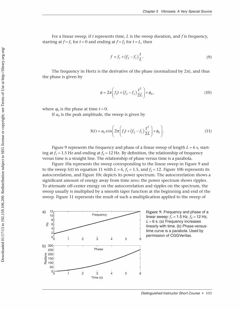
Figure 9 represents the frequency and phase of a linear sweep of length L = 6 s, start-ing at f1 = 1.5 Hz and ending at f2 = 12 Hz. By definition, the relationship of frequency versus time is a straight line. The relationship of phase versus time is a parabola.

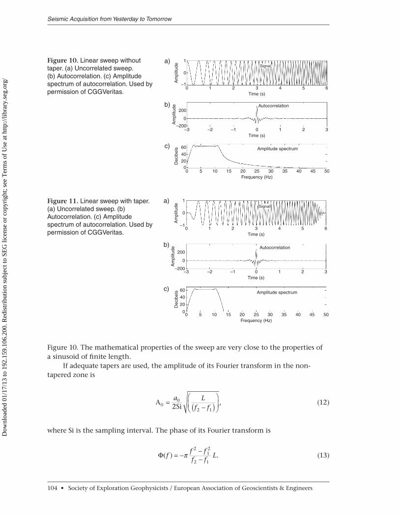
Figure 10a represents the sweep corresponding to the linear sweep in Figure 9 and to the sweep S(t) in equation 11 with L = 6, f1 = 1.5, and f2 = 12. Figure 10b represents its autocorrelation, and Figure 10c depicts its power spectrum. The autocorrelation shows a significant amount of energy away from time zero; the power spectrum shows ripples. To attenuate off-center energy on the autocorrelation and ripples on the spectrum, the sweep usually is multiplied by a smooth taper function at the beginning and end of the sweep. Figure 11 represents the result of such a multiplication applied to the sweep of



12a)Frequency

Phase

Time (s)

1086H

z

420

300b)250200150

Rad

ians

100500

0 1 2 3 4 5 6

0 1 2 3 4 5 6

Figure 9. Frequency and phase of a linear sweep: f1 = 1.5 Hz, f2 = 12 Hz, L = 6 s. (a) Frequency increases linearly with time. (b) Phase-versus-time curve is a parabola. Used by permission of CGGVeritas.

Dow

nloa

ded

01/1

7/13

to 1

92.1

59.1

06.2

00. R

edis

trib

utio

n su

bjec

t to

SEG

lice

nse

or c

opyr

ight

; see

Ter

ms

of U

se a

t http

://lib

rary

.seg

.org

/



Figure 10. The mathematical properties of the sweep are very close to the properties of a sinusoid of finite length.

If adequate tapers are used, the amplitude of its Fourier transform in the non-tapered zone is

ASi0 =

-( )Ê

ËÁˆ

¯̃a L

f f0

2 12,

(12)

where Si is the sampling interval. The phase of its Fourier transform is

F( ) .f

f ff f

L= - --p

212

2 1 (13)

1a)

b)

0

Am

plitu

de

–1

–3 –2 –1 0 1 2 3

200

0

Am

plitu

de

–200

c) 60

40

Dec

ibel

s

20

00 5 10 15 20 25 30 35 40 45 50

0 1 2 3 4 5Time (s)

Time (s)

Frequency (Hz)

Autocorrelation

Amplitude spectrum

Signal

6

Figure 11. Linear sweep with taper. (a) Uncorrelated sweep. (b) Autocorrelation. (c) Amplitude spectrum of autocorrelation. Used by permission of CGGVeritas.

1a)

b)

0

Am

plitu

de

–1

–3 –2 –1 0 1 2 3

200

0

Am

plitu

de

–200

c) 60

40

Dec

ibel

s

2000 5 10 15 20 25 30 35 40 45 50

0 1 2 3 4 5Time (s)

Time (s)

Frequency (Hz)

Autocorrelation

Amplitude spectrum

Signal

6

Figure 10. Linear sweep without taper. (a) Uncorrelated sweep. (b) Autocorrelation. (c) Amplitude spectrum of autocorrelation. Used by permission of CGGVeritas.

Dow

nloa

ded

01/1

7/13

to 1

92.1

59.1

06.2

00. R

edis

trib

utio

n su

bjec

t to

SEG

lice

nse

or c

opyr

ight

; see

Ter

ms

of U

se a

t http

://lib

rary

.seg

.org

/

The maximum of its autocorrelation is

A

Sic = aL

02

2.

(14)

Until the late 1970s, linear sweeps were the only option available with current equip-ment. Advances in electronic equipment have made nonlinear sweeps available to tilt the signal spectrum upward or downward. The basic parameter that controls nonlinear sweep is the sweep rate, the derivative of the sweep frequency relative to time:

Sr( )

( ).t

df tdt

=

(15)

For a linear sweep,

Sr( )t

f fL

= -2 1

(16)

is constant. The generalized formula for the amplitude spectrum of a (constant ampli-tude) sweep is

A

Si Sr0( )( )

.fa

f= Ê

ËÁˆ¯̃

0

21

(17)

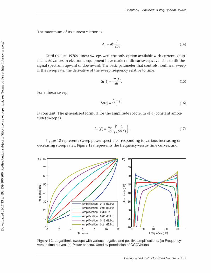
Figure 12 represents sweep power spectra corresponding to various increasing or decreasing sweep rates. Figure 12a represents the frequency-versus-time curves, and



80a)

70

60

50

Freq

uenc

y (H

z)

40

30

20

10

0

60b)

55

50

45

Am

plitu

de (

dB)

40

35

30

25

200 2 4 6

Amplification –0.16 dB/Hz

Amplification 0.16 dB/Hz


Amplification –0.08 dB/Hz


Amplification 0 dB/Hz

Time (s)

8 0 20 40 60

Frequency (Hz)

8010 12

Figure 12. Logarithmic sweeps with various negative and positive amplifications. (a) Frequency-versus-time curves. (b) Power spectra. Used by permission of CGGVeritas.

Dow

nloa

ded

01/1

7/13

to 1

92.1

59.1

06.2

00. R

edis

trib

utio

n su

bjec

t to

SEG

lice

nse

or c

opyr

ight

; see

Ter

ms

of U

se a

t http

://lib

rary

.seg

.org

/

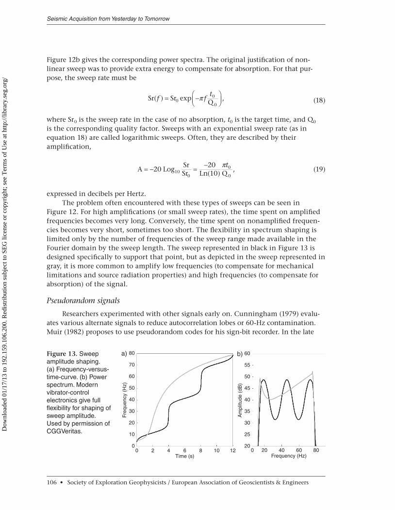
Figure 12b gives the corresponding power spectra. The original justification of non-linear sweep was to provide extra energy to compensate for absorption. For that pur-pose, the sweep rate must be

Sr Sr

Q( ) exp ,f f

t= -ÊËÁ

ˆ¯̃0

0

0π

(18)

where Sr0 is the sweep rate in the case of no absorption, t0 is the target time, and Q0 is the corresponding quality factor. Sweeps with an exponential sweep rate (as in equation 18) are called logarithmic sweeps. Often, they are described by their amplification,

A Log

SrSr Ln Q

= - = -20

201010

0

0

0( ),

πt

(19)

expressed in decibels per Hertz.The problem often encountered with these types of sweeps can be seen in

Figure 12. For high amplifications (or small sweep rates), the time spent on amplified frequencies becomes very long. Conversely, the time spent on nonamplified frequen-cies becomes very short, sometimes too short. The flexibility in spectrum shaping is limited only by the number of frequencies of the sweep range made available in the Fourier domain by the sweep length. The sweep represented in black in Figure 13 is designed specifically to support that point, but as depicted in the sweep represented in gray, it is more common to amplify low frequencies (to compensate for mechanical limitations and source radiation properties) and high frequencies (to compensate for absorption) of the signal.

Pseudorandom signals

Researchers experimented with other signals early on. Cunningham (1979) evalu-ates various alternate signals to reduce autocorrelation lobes or 60-Hz contamination. Muir (1982) proposes to use pseudorandom codes for his sign-bit recorder. In the late



80

70

60

50

40

Freq

uenc

y (H

z)

30

20

10

00 2 4 6

Time (s)8 0 20 40 60

Frequency (Hz)8010 12

a) 60

55

50

45

40

Am

plitu

de (

dB)

35

30

25

20

b)Figure 13. Sweep amplitude shaping. (a) Frequency-versus-time-curve. (b) Power spectrum. Modern vibrator-control electronics give full flexibility for shaping of sweep amplitude. Used by permission of CGGVeritas.D

ownl

oade

d 01

/17/

13 to

192

.159

.106

.200

. Red

istr

ibut

ion

subj

ect t

o SE

G li

cens

e or

cop

yrig

ht; s

ee T

erm

s of

Use

at h

ttp://

libra

ry.s

eg.o

rg/

1980s, digital-control electronics made pseudorandom signals (curiously, sometimes also called random sweeps) as easy to use as conventional sweeps. One possible imple-mentation (Burger et al., 1992) is to use a binary shift register to generate a maximum-length pseudorandom binary sequence (PRBS). The PRBS output of the shift register then is filtered to the desired bandwidth.

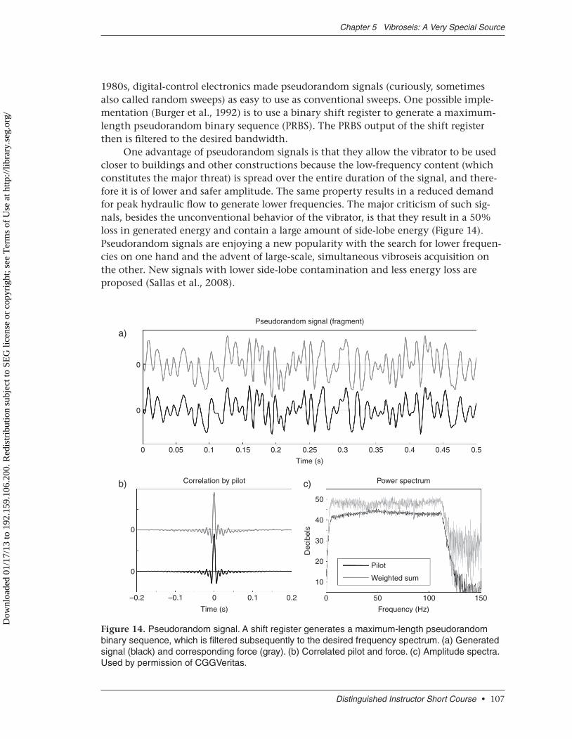
One advantage of pseudorandom signals is that they allow the vibrator to be used closer to buildings and other constructions because the low-frequency content (which constitutes the major threat) is spread over the entire duration of the signal, and there-fore it is of lower and safer amplitude. The same property results in a reduced demand for peak hydraulic flow to generate lower frequencies. The major criticism of such sig-nals, besides the unconventional behavior of the vibrator, is that they result in a 50% loss in generated energy and contain a large amount of side-lobe energy (Figure 14). Pseudorandom signals are enjoying a new popularity with the search for lower frequen-cies on one hand and the advent of large-scale, simultaneous vibroseis acquisition on the other. New signals with lower side-lobe contamination and less energy loss are proposed (Sallas et al., 2008).



0

50

40

30

Dec

ibel

s

20 Pilot

Weighted sum10

0 50 100

Frequency (Hz)

150

0

–0.2 –0.1 0.1 0.20

Time (s)

Correlation by pilotb) c) Power spectrum

Pseudorandom signal (fragment)

0

0

0 0.05 0.1

a)

0.15 0.2 0.25

Time (s)

0.3 0.35 0.4 0.45 0.5

Figure 14. Pseudorandom signal. A shift register generates a maximum-length pseudorandom binary sequence, which is filtered subsequently to the desired frequency spectrum. (a) Generated signal (black) and corresponding force (gray). (b) Correlated pilot and force. (c) Amplitude spectra. Used by permission of CGGVeritas.

Dow

nloa

ded

01/1

7/13

to 1

92.1

59.1

06.2

00. R

edis

trib

utio

n su

bjec

t to

SEG

lice

nse

or c

opyr

ight

; see

Ter

ms

of U

se a

t http

://lib

rary

.seg

.org

/

Relationship between vibrator motion and far-field signal

Miller and Pursey (1954) show that for a homogeneous, lossless elastic half-space in the far field, the time-shifted particle displacement is proportional to the stress gener-ated by a disk of finite radius vibrating normally to the surface of the half-space. In other words, a semi-infinite homogeneous elastic medium behaves like a spring.

In their comments to Lerwill, Sallas and Weber (1982) show that the weighted sum of the reaction mass and baseplate accelerations is an adequate representation of the ground force and should be used for vibrator control. The weighted sum provides an approximation of the vibrator signal or, more precisely, of its displacement component.

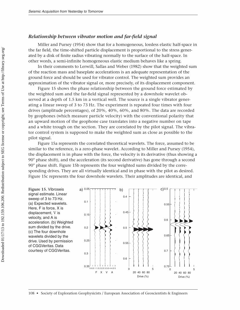
Figure 15 shows the phase relationship between the ground force estimated by the weighted sum and the far-field signal represented by a downhole wavelet ob-served at a depth of 1.5 km in a vertical well. The source is a single vibrator gener-ating a linear sweep of 3 to 73 Hz. The experiment is repeated four times with four drives (amplitude percentages), of 20%, 40%, 60%, and 80%. The data are recorded by geophones (which measure particle velocity) with the conventional polarity that an upward motion of the geophone case translates into a negative number on tape and a white trough on the section. They are correlated by the pilot signal. The vibra-tor control system is supposed to make the weighted sum as close as possible to the pilot signal.

Figure 15a represents the correlated theoretical wavelets. The force, assumed to be similar to the reference, is a zero-phase wavelet. According to Miller and Pursey (1954), the displacement is in phase with the force, the velocity is its derivative (thus showing a 90° phase shift), and the acceleration (its second derivative) has gone through a second 90° phase shift. Figure 15b represents the four weighted sums divided by the corre-sponding drives. They are all virtually identical and in phase with the pilot as desired. Figure 15c represents the four downhole wavelets. Their amplitudes are identical, and



0.05a)

0.4

0.45

0.5

0.55

0.6

0 5

b)

0.1

0.15

0.2

0.25

0.3

0.35

0.5c)

0.55

0.6

0.65

0.7

0.75

F X V A 20 40 60

Drive (%)

800 5

20 40 60

Drive (%)

80

0 0.5 1 1.5 2 2.5 3 3.5 4 4.5 5

Figure 15. Vibroseis signal estimate. Linear sweep of 3 to 73 Hz. (a) Expected wavelets. Here, F is force, X is displacement, V is velocity, and A is acceleration. (b) Weighted sum divided by the drive. (c) The four downhole wavelets divided by the drive. Used by permission of CGGVeritas. Data courtesy of CGGVeritas.

Dow

nloa

ded

01/1

7/13

to 1

92.1

59.1

06.2

00. R

edis

trib

utio

n su

bjec

t to

SEG

lice

nse

or c

opyr

ight

; see

Ter

ms

of U

se a

t http

://lib

rary

.seg

.org

/

their phases are very close to the phase of the velocity wavelet shown in Figure 15a, in good agreement with the theory.

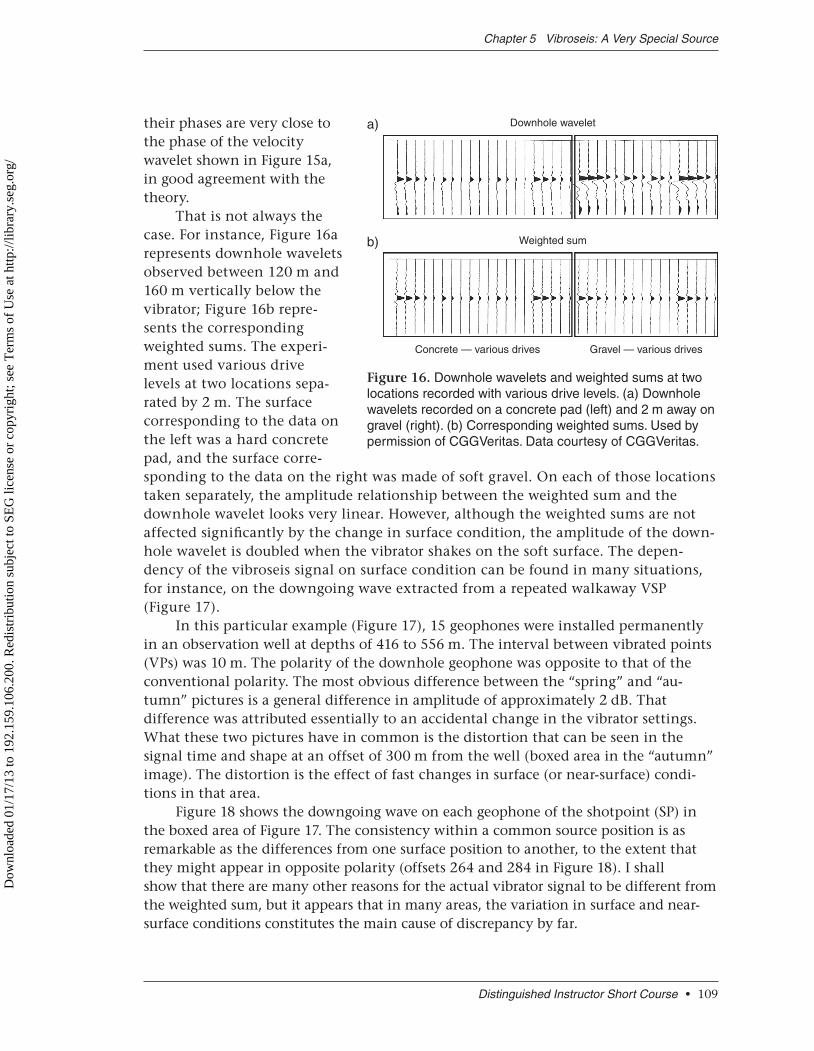
That is not always the case. For instance, Figure 16a represents downhole wavelets observed between 120 m and 160 m vertically below the vibrator; Figure 16b repre-sents the corresponding weighted sums. The experi-ment used various drive levels at two locations sepa-rated by 2 m. The surface corresponding to the data on the left was a hard concrete pad, and the surface corre-sponding to the data on the right was made of soft gravel. On each of those locations taken separately, the amplitude relationship between the weighted sum and the downhole wavelet looks very linear. However, although the weighted sums are not affected significantly by the change in surface condition, the amplitude of the down-hole wavelet is doubled when the vibrator shakes on the soft surface. The depen-dency of the vibroseis signal on surface condition can be found in many situations, for instance, on the downgoing wave extracted from a repeated walkaway VSP (Figure 17).

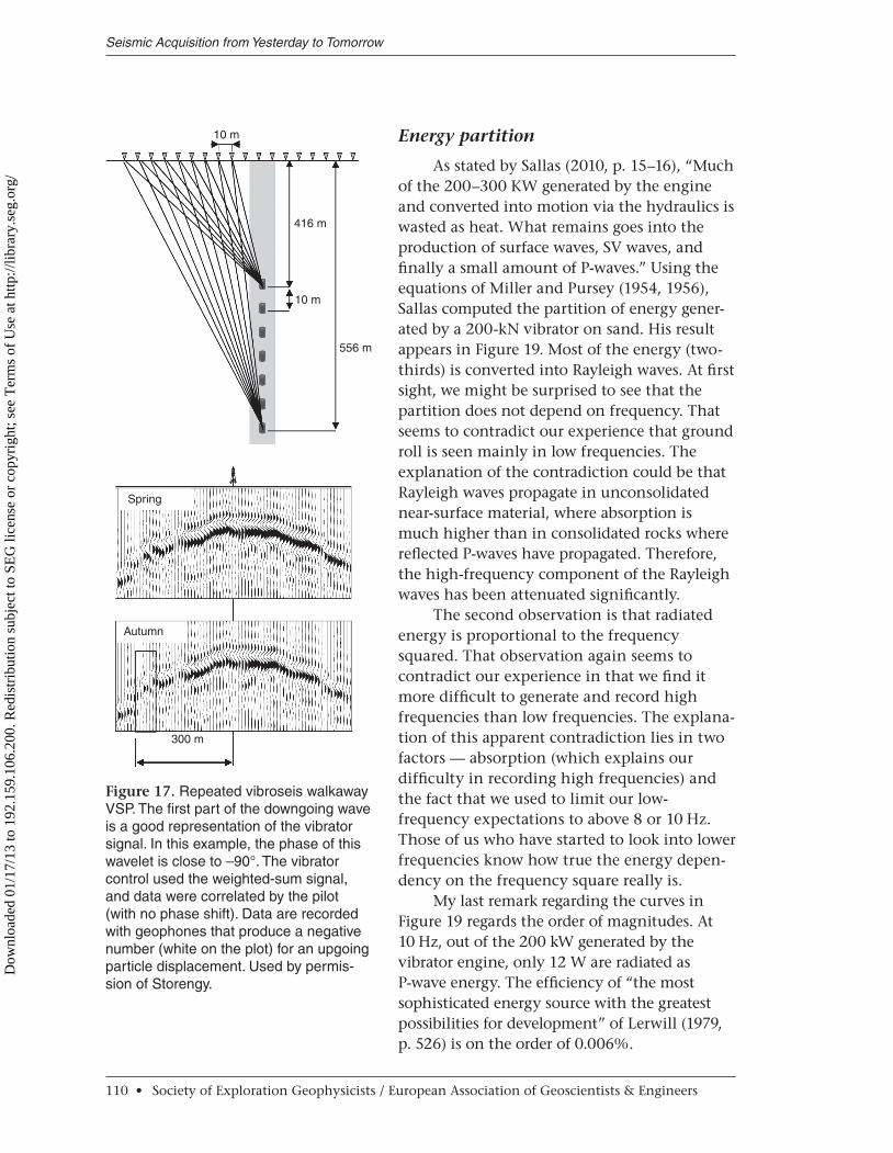
In this particular example (Figure 17), 15 geophones were installed permanently in an observation well at depths of 416 to 556 m. The interval between vibrated points (VPs) was 10 m. The polarity of the downhole geophone was opposite to that of the conventional polarity. The most obvious difference between the “spring” and “au-tumn” pictures is a general difference in amplitude of approximately 2 dB. That difference was attributed essentially to an accidental change in the vibrator settings. What these two pictures have in common is the distortion that can be seen in the signal time and shape at an offset of 300 m from the well (boxed area in the “autumn” image). The distortion is the effect of fast changes in surface (or near-surface) condi-tions in that area.

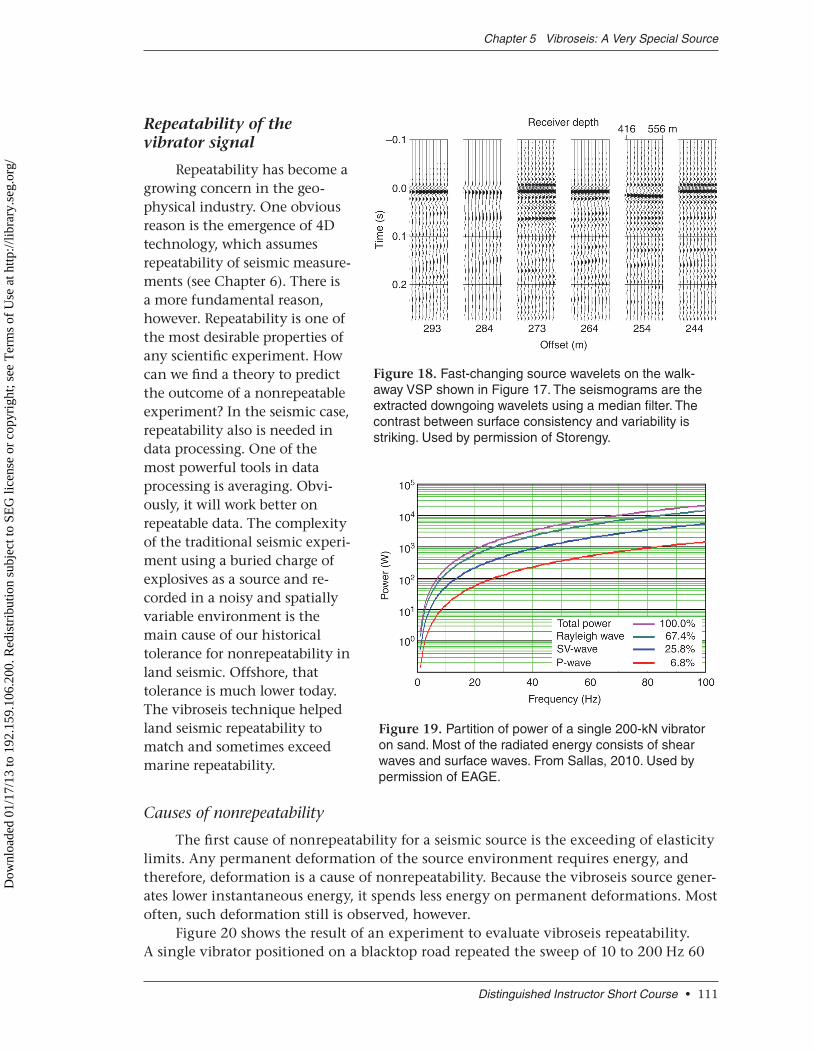
Figure 18 shows the downgoing wave on each geophone of the shotpoint (SP) in the boxed area of Figure 17. The consistency within a common source position is as remarkable as the differences from one surface position to another, to the extent that they might appear in opposite polarity (offsets 264 and 284 in Figure 18). I shall show that there are many other reasons for the actual vibrator signal to be different from the weighted sum, but it appears that in many areas, the variation in surface and near-surface conditions constitutes the main cause of discrepancy by far.



Downhole waveleta)

Weighted sum

Concrete — various drives Gravel — various drives

b)

Figure 16. Downhole wavelets and weighted sums at two locations recorded with various drive levels. (a) Downhole wavelets recorded on a concrete pad (left) and 2 m away on gravel (right). (b) Corresponding weighted sums. Used by permission of CGGVeritas. Data courtesy of CGGVeritas.

Dow

nloa

ded

01/1

7/13

to 1

92.1

59.1

06.2

00. R

edis

trib

utio

n su

bjec

t to

SEG

lice

nse

or c

opyr

ight

; see

Ter

ms

of U

se a

t http

://lib

rary

.seg

.org

/

Energy partition

As stated by Sallas (2010, p. 15–16), “Much of the 200–300 KW generated by the engine and converted into motion via the hydraulics is wasted as heat. What remains goes into the production of surface waves, SV waves, and finally a small amount of P-waves.” Using the equations of Miller and Pursey (1954, 1956), Sallas computed the partition of energy gener-ated by a 200-kN vibrator on sand. His result appears in Figure 19. Most of the energy (two-thirds) is converted into Rayleigh waves. At first sight, we might be surprised to see that the partition does not depend on frequency. That seems to contradict our experience that ground roll is seen mainly in low frequencies. The explanation of the contradiction could be that Rayleigh waves propagate in unconsolidated near-surface material, where absorption is much higher than in consolidated rocks where reflected P-waves have propagated. Therefore, the high-frequency component of the Rayleigh waves has been attenuated significantly.

The second observation is that radiated energy is proportional to the frequency squared. That observation again seems to contradict our experience in that we find it more difficult to generate and record high frequencies than low frequencies. The explana-tion of this apparent contradiction lies in two factors — absorption (which explains our difficulty in recording high frequencies) and the fact that we used to limit our low- frequency expectations to above 8 or 10 Hz. Those of us who have started to look into lower frequencies know how true the energy depen-dency on the frequency square really is.

My last remark regarding the curves in Figure 19 regards the order of magnitudes. At 10 Hz, out of the 200 kW generated by the vibrator engine, only 12 W are radiated as P-wave energy. The efficiency of “the most sophisticated energy source with the greatest possibilities for development” of Lerwill (1979, p. 526) is on the order of 0.006%.



10 m

416 m

10 m

300 m

Spring

Autumn

556 m

Figure 17. Repeated vibroseis walkaway VSP. The first part of the downgoing wave is a good representation of the vibrator signal. In this example, the phase of this wavelet is close to –90°. The vibrator control used the weighted-sum signal, and data were correlated by the pilot (with no phase shift). Data are recorded with geophones that produce a negative number (white on the plot) for an upgoing particle displacement. Used by permis-sion of Storengy.

Dow

nloa

ded

01/1

7/13

to 1

92.1

59.1

06.2

00. R

edis

trib

utio

n su

bjec

t to

SEG

lice

nse

or c

opyr

ight

; see

Ter

ms

of U

se a

t http

://lib

rary

.seg

.org

/

Repeatability of the vibrator signal

Repeatability has become a growing concern in the geo-physical industry. One obvious reason is the emergence of 4D technology, which assumes repeatability of seismic measure-ments (see Chapter 6). There is a more fundamental reason, however. Repeatability is one of the most desirable properties of any scientific experiment. How can we find a theory to predict the outcome of a nonrepeatable experiment? In the seismic case, repeatability also is needed in data processing. One of the most powerful tools in data processing is averaging. Obvi-ously, it will work better on repeatable data. The complexity of the traditional seismic experi-ment using a buried charge of explosives as a source and re-corded in a noisy and spatially variable environment is the main cause of our historical tolerance for nonrepeatability in land seismic. Offshore, that tolerance is much lower today. The vibroseis technique helped land seismic repeatability to match and sometimes exceed marine repeatability.

Causes of nonrepeatability

The first cause of nonrepeatability for a seismic source is the exceeding of elasticity limits. Any permanent deformation of the source environment requires energy, and therefore, deformation is a cause of nonrepeatability. Because the vibroseis source gener-ates lower instantaneous energy, it spends less energy on permanent deformations. Most often, such deformation still is observed, however.

Figure 20 shows the result of an experiment to evaluate vibroseis repeatability. A single vibrator positioned on a blacktop road repeated the sweep of 10 to 200 Hz 60



Figure 18. Fast-changing source wavelets on the walk-away VSP shown in Figure 17. The seismograms are the extracted downgoing wavelets using a median filter. The contrast be tween surface consistency and variability is striking. Used by permission of Storengy.

Figure 19. Partition of power of a single 200-kN vibrator on sand. Most of the radiated energy consists of shear waves and surface waves. From Sallas, 2010. Used by permission of EAGE.

Dow

nloa

ded

01/1

7/13

to 1

92.1

59.1

06.2

00. R

edis

trib

utio

n su

bjec

t to

SEG

lice

nse

or c

opyr

ight

; see

Ter

ms

of U

se a

t http

://lib

rary

.seg

.org

/

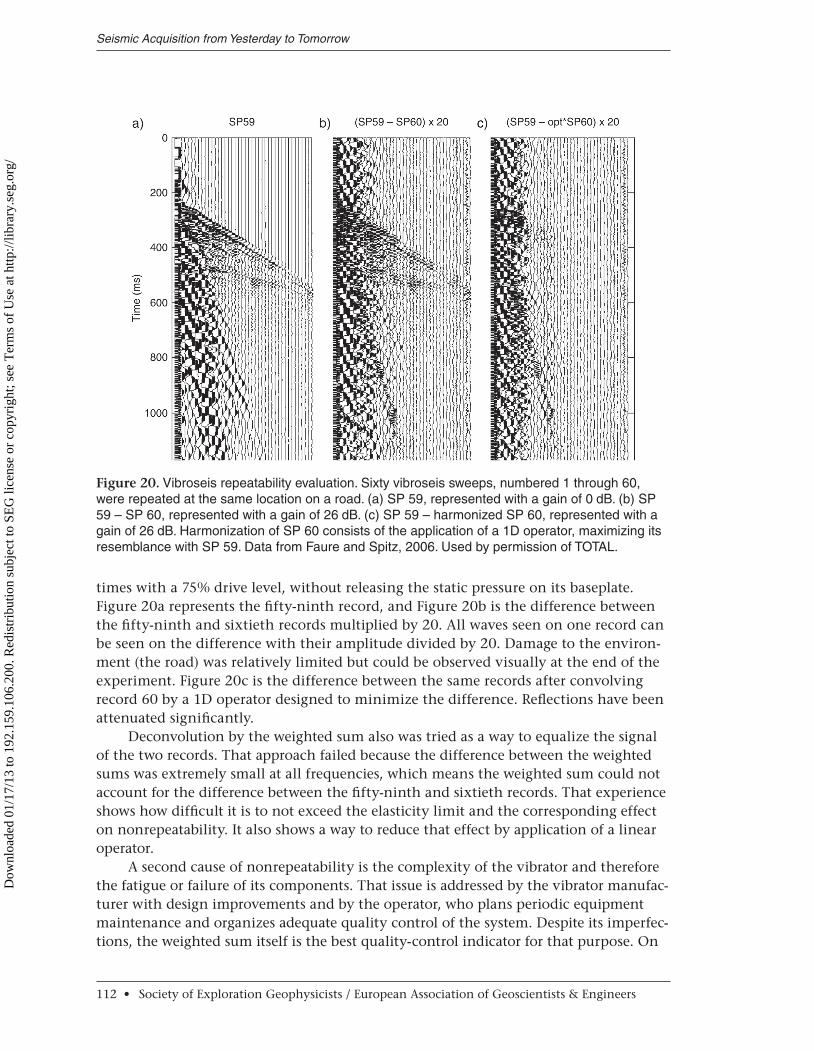
times with a 75% drive level, without releasing the static pressure on its baseplate. Figure 20a represents the fifty-ninth record, and Figure 20b is the difference between the fifty-ninth and sixtieth records multiplied by 20. All waves seen on one record can be seen on the difference with their amplitude divided by 20. Damage to the environ-ment (the road) was relatively limited but could be observed visually at the end of the experiment. Figure 20c is the difference between the same records after convolving record 60 by a 1D operator designed to minimize the difference. Reflections have been attenuated significantly.

Deconvolution by the weighted sum also was tried as a way to equalize the signal of the two records. That approach failed because the difference between the weighted sums was extremely small at all frequencies, which means the weighted sum could not account for the difference between the fifty-ninth and sixtieth records. That experience shows how difficult it is to not exceed the elasticity limit and the corresponding effect on nonrepeatability. It also shows a way to reduce that effect by application of a linear operator.

A second cause of nonrepeatability is the complexity of the vibrator and therefore the fatigue or failure of its components. That issue is addressed by the vibrator manufac-turer with design improvements and by the operator, who plans periodic equipment maintenance and organizes adequate quality control of the system. Despite its imperfec-tions, the weighted sum itself is the best quality-control indicator for that purpose. On



Figure 20. Vibroseis repeatability evaluation. Sixty vibroseis sweeps, numbered 1 through 60, were repeated at the same location on a road. (a) SP 59, represented with a gain of 0 dB. (b) SP 59 – SP 60, represented with a gain of 26 dB. (c) SP 59 – harmonized SP 60, represented with a gain of 26 dB. Harmonization of SP 60 consists of the application of a 1D operator, maximizing its resemblance with SP 59. Data from Faure and Spitz, 2006. Used by permission of TOTAL.

Dow

nloa

ded

01/1

7/13

to 1

92.1

59.1

06.2

00. R

edis

trib

utio

n su

bjec

t to

SEG

lice

nse

or c

opyr

ight

; see

Ter

ms

of U

se a

t http

://lib

rary

.seg

.org

/

many crews today, weighted sums are recorded for each vibration of each vibrator and subsequently are analyzed for quality control.

The last cause of nonrepeatability is the most difficult to deal with and has not been addressed satisfactorily as of this writing — variability of surface conditions. That is by far the most significant cause of nonrepeatability. A possible, albeit expensive and imperfect, way to reduce the effect of surface-condition variability is to use permanent seismic systems.

How can repeatability be improved?

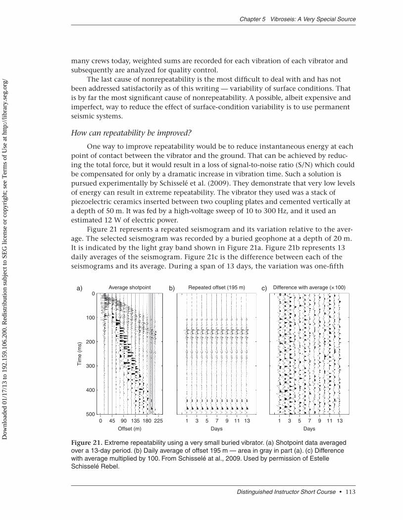
One way to improve repeatability would be to reduce instantaneous energy at each point of contact between the vibrator and the ground. That can be achieved by reduc-ing the total force, but it would result in a loss of signal-to-noise ratio (S/N) which could be compensated for only by a dramatic increase in vibration time. Such a solution is pursued experimentally by Schisselé et al. (2009). They demonstrate that very low levels of energy can result in extreme repeatability. The vibrator they used was a stack of piezoelectric ceramics inserted between two coupling plates and cemented vertically at a depth of 50 m. It was fed by a high-voltage sweep of 10 to 300 Hz, and it used an estimated 12 W of electric power.

Figure 21 represents a repeated seismogram and its variation relative to the aver-age. The selected seismogram was recorded by a buried geophone at a depth of 20 m. It is indicated by the light gray band shown in Figure 21a. Figure 21b represents 13 daily averages of the seismogram. Figure 21c is the difference between each of the seismograms and its average. During a span of 13 days, the variation was one-fifth



0Average shotpointa) Repeated offset (195 m)b)

100

200

Tim

e (m

s)

300

400

5000 45 90 135

Offset (m)

180 225 1 3 5 7

Days

9 11 13

Difference with average (× 100)c)

1 3 5 7

Days

9 11 13

Figure 21. Extreme repeatability using a very small buried vibrator. (a) Shotpoint data averaged over a 13-day period. (b) Daily average of offset 195 m — area in gray in part (a). (c) Difference with average multiplied by 100. From Schisselé at al., 2009. Used by permission of Estelle Schisselé Rebel.

Dow

nloa

ded

01/1

7/13

to 1

92.1

59.1

06.2

00. R

edis

trib

utio

n su

bjec

t to

SEG

lice

nse

or c

opyr

ight

; see

Ter

ms

of U

se a

t http

://lib

rary

.seg

.org

/

that of a conventional vibrator between two consecutive sweeps. It must be noted that a large part of the repeatability enhancement is associated with the depth of operation of the source and (to a lesser degree) of the receiver. Away from the earth surface, the mechanical properties of the rocks no longer are affected by weather-related variations.

The second solution, to increase the surface of contact with the ground, is made difficult by insufficient stiffness of the baseplate or by resolution loss that would result from use of a larger source array.

Vibroseis signal and noise

Chapter 4 showed that summations of signal and noise have different properties. That fact is certainly true for any seismic source. What makes the vibroseis source special is the fact that signal at any frequency can be generated in a longer or shorter period of time and that noise also is recorded during that time. Therefore, the vibroseis technique provides some leverage on S/N. To analyze the leverage, I shall make a few assumptions that will be discussed. From those assumptions, I will derive a law describ-ing the behavior of signal and ambient noise in the imaging process for vibroseis data.

Assumptions

First, I assume that wave propagation is linear. That assumption has an obvious upper limit: When a very large signal is generated, some damage to the environment occurs, as noted above. Damage is not linear. It is worth repeating here that the vibro-seis source, with its relatively modest amplitude, honors the assumption of linearity more than many other seismic sources do. Whether there is a lower limit to the assump-tion is not known. As far as I know, the question, “Is there a threshold below which wave propagation stops?” remains unanswered. An investigation of a possible threshold was described in Chapter 4, in the section entitled “Order of magnitude.” No threshold was found. Following the experiment described in Chapter 4, I shall assume there is no lower limit to the linearity of wave propagation. A consequence of that absence is that penetration, “[t]he greatest depth from which seismic reflections can be picked with reasonable certainty” (Sheriff, 1981, p. 259), is only a function of the signal-to-noise ratio. If we can increase S/N, we can see to lower depths. Note that in the above state-ment, noise is not restricted to ambient noise — it is taken in a more general sense.

Next, I assume that in an ideal seismic sum, at any given frequency, signal is pro-portional to the number of terms. That assumption simply means that after possible alignment, signal wavelength is large compared with the array formed by the summed seismograms.

Finally, I assume that in an ideal seismic sum, at any given frequency, ambient noise is proportional to the square root of the number of terms. In fact, that assumption is very similar to the assumption that ambient noise has constant rms amplitude and is uncorrelated. The assumption that in an ideal seismic sum, at any given frequency, ambient noise is proportional to the square root of the number of terms might seem quite restrictive. However, ambient noise measured on a given receiver at different times most often shows a very low degree of correlation.



Dow

nloa

ded

01/1

7/13

to 1

92.1

59.1

06.2

00. R

edis

trib

utio

n su

bjec

t to

SEG

lice

nse

or c

opyr

ight

; see

Ter

ms

of U

se a

t http

://lib

rary

.seg

.org

/

Signal and noise behavior

In Chapter 4, I showed that the reference in which to evaluate signal and noise in the seismic image is not the arbitrary 3D bin but the physical unit of surface. From now on, for the sake of simplicity, signal and noise will refer to signal and ambient noise per unit of surface. It also was shown that at any given frequency, S/N was proportional to the signal strength estimator (SSE) (equation 12 of Chapter 4, reproduced below):

SSE Ss SD NR RA( ) ( ) * * ,f f= (20)

where RA is the area of the receiver station, NR is the number of receiver per shotpoint, and SD is the source density (number of shotpoints per surface unit). Here, Ss(f ) is the source strength. It is the amplitude of the far-field signal generated by a single source, and it usually depends on frequency. In vibroseis operations, using the above three assump-tions, source strength Ss(f ) can be expressed as a function of the source parameters.

From assumptions one and two above, at any given frequency, signal is proportional to the ground force applied at that frequency and to the time spent emitting that frequency (inverse sweep rate). Proportionality to the time spent is a natural consequence of linearity: A signal of length L can be seen as L signals of unit length. Those signals are summed subsequently. For the same reason and following assumption three above, at any given frequency, noise is proportional to the square root of the time spent emitting that frequency (inverse sweep rate, or dwell). That can be expressed by the equations

Signal( Pf D Nvf

f)

( )ª Ê

ËÁˆ¯̃

1Sr

(21)

and

Noise( )

( ).f

fª 1

Sr

(22)

Consequently,

Ss( )

( ),f

f= Pf D Nv

Sr1

(23)

where Pf is the vibrator peak force, D is the drive, Nv is the number of vibrators, and Sr(f ) is the sweep rate df/dt.

Figure 22 illustrates the relationship among sweep rate, signal, and noise. In the figure, the signal is a logarithmic sweep of length L = 10 s with an amplification of 0.25 dB/Hz, and the noise is a sum of sinusoids of equal amplitude, of frequencies multiple of 1/L, and of random phase. The solid black curve represents the amplitude spectrum of the correlation of the signal by the sweep. It is parallel (and therefore proportional) to the inverse sweep rate (dashed black line). The solid gray curve represents the amplitude spectrum of the correlation of the noise by the sweep. It



Dow

nloa

ded

01/1

7/13

to 1

92.1

59.1

06.2

00. R

edis

trib

utio

n su

bjec

t to

SEG

lice

nse

or c

opyr

ight

; see

Ter

ms

of U

se a

t http

://lib

rary

.seg

.org

/

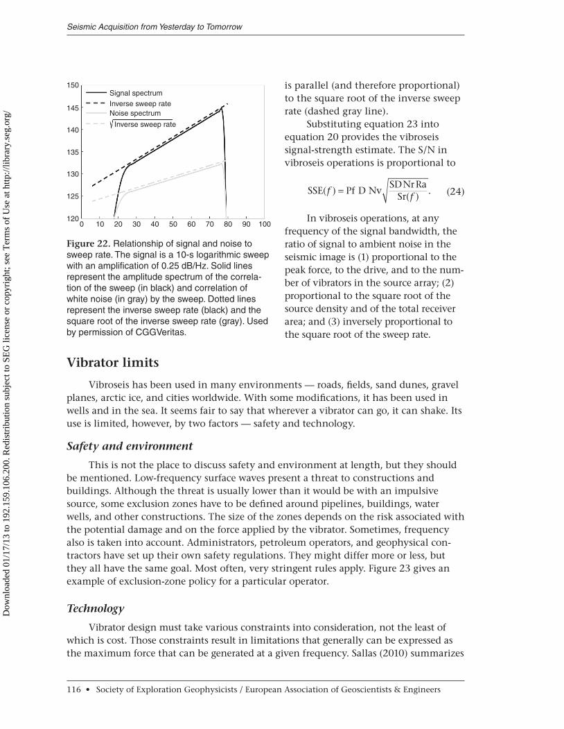
is parallel (and therefore proportional) to the square root of the inverse sweep rate (dashed gray line).

Substituting equation 23 into equation 20 provides the vibroseis signal-strength estimate. The S/N in vibroseis operations is proportional to

SSE Pf NvSDNrRa

Sr( )

( ).f

f= D (24)

In vibroseis operations, at any frequency of the signal bandwidth, the ratio of signal to ambient noise in the seismic image is (1) proportional to the peak force, to the drive, and to the num-ber of vibrators in the source array; (2) proportional to the square root of the source density and of the total receiver area; and (3) inversely proportional to the square root of the sweep rate.

Vibrator limits

Vibroseis has been used in many environments — roads, fields, sand dunes, gravel planes, arctic ice, and cities worldwide. With some modifications, it has been used in wells and in the sea. It seems fair to say that wherever a vibrator can go, it can shake. Its use is limited, however, by two factors — safety and technology.

Safety and environment

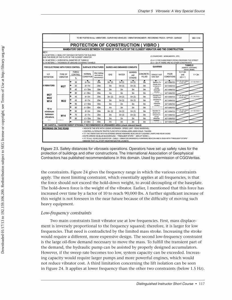
This is not the place to discuss safety and environment at length, but they should be mentioned. Low-frequency surface waves present a threat to constructions and buildings. Although the threat is usually lower than it would be with an impulsive source, some exclusion zones have to be defined around pipelines, buildings, water wells, and other constructions. The size of the zones depends on the risk associated with the potential damage and on the force applied by the vibrator. Sometimes, frequency also is taken into account. Administrators, petroleum operators, and geophysical con-tractors have set up their own safety regulations. They might differ more or less, but they all have the same goal. Most often, very stringent rules apply. Figure 23 gives an example of exclusion-zone policy for a particular operator.

Technology

Vibrator design must take various constraints into consideration, not the least of which is cost. Those constraints result in limitations that generally can be expressed as the maximum force that can be generated at a given frequency. Sallas (2010) summarizes



150

145

140

135

130

125

1200 10 20 30 40 50 60 70 80 90 100

Signal spectrumInverse sweep rateNoise spectrum

Inverse sweep rate

Figure 22. Relationship of signal and noise to sweep rate. The signal is a 10-s logarithmic sweep with an amplification of 0.25 dB/Hz. Solid lines represent the amplitude spectrum of the correla-tion of the sweep (in black) and correlation of white noise (in gray) by the sweep. Dotted lines represent the inverse sweep rate (black) and the square root of the inverse sweep rate (gray). Used by permission of CGGVeritas.

Dow

nloa

ded

01/1

7/13

to 1

92.1

59.1

06.2

00. R

edis

trib

utio

n su

bjec

t to

SEG

lice

nse

or c

opyr

ight

; see

Ter

ms

of U

se a

t http

://lib

rary

.seg

.org

/

the constraints. Figure 24 gives the frequency range in which the various constraints apply. The most limiting constraint, which essentially applies at all frequencies, is that the force should not exceed the hold-down weight, to avoid decoupling of the baseplate. The hold-down force is the weight of the vibrator. Earlier, I mentioned that this force has increased over time by a factor of 10 to reach 90,000 lbs. A further significant increase of this weight is not foreseen in the near future because of the difficulty of moving such heavy equipment.

Low-frequency constraints

Two main constraints limit vibrator use at low frequencies. First, mass displace-ment is inversely proportional to the frequency squared; therefore, it is larger for low frequencies. That need is contradicted by the limited mass stroke. Increasing the stroke would require a different, more expensive design. The second low-frequency constraint is the large oil-flow demand necessary to move the mass. To fulfill the transient part of the demand, the hydraulic pump can be assisted by properly designed accumulators. However, if the sweep rate becomes too low, system capacity can be exceeded. Increas-ing capacity would require larger pumps and more powerful engines, which would not reduce vibrator cost. A third limitation concerning the lift isolation can be seen in Figure 24. It applies at lower frequency than the other two constraints (below 1.5 Hz).



Figure 23. Safety distances for vibroseis operations. Operators have set up safety rules for the protection of buildings and other constructions. The International Association of Geophysical Contractors has published recommendations in this domain. Used by permission of CGGVeritas.

Dow

nloa

ded

01/1

7/13

to 1

92.1

59.1

06.2

00. R

edis

trib

utio

n su

bjec

t to

SEG

lice

nse

or c

opyr

ight

; see

Ter

ms

of U

se a

t http

://lib

rary

.seg

.org

/

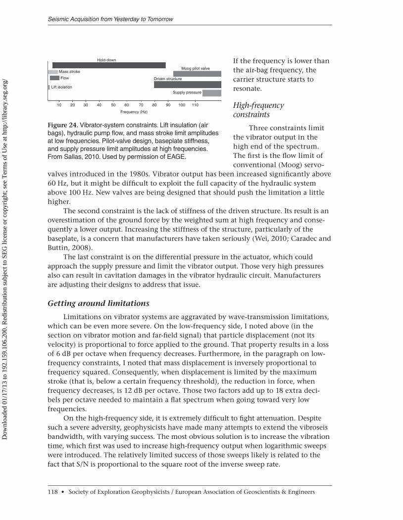
If the frequency is lower than the air-bag frequency, the carrier structure starts to resonate.

High-frequency constraints

Three constraints limit the vibrator output in the high end of the spectrum. The first is the flow limit of conventional (Moog) servo-

valves introduced in the 1980s. Vibrator output has been increased significantly above 60 Hz, but it might be difficult to exploit the full capacity of the hydraulic system above 100 Hz. New valves are being designed that should push the limitation a little higher.

The second constraint is the lack of stiffness of the driven structure. Its result is an overestimation of the ground force by the weighted sum at high frequency and conse-quently a lower output. Increasing the stiffness of the structure, particularly of the baseplate, is a concern that manufacturers have taken seriously (Wei, 2010; Caradec and Buttin, 2008).

The last constraint is on the differential pressure in the actuator, which could approach the supply pressure and limit the vibrator output. Those very high pressures also can result in cavitation damages in the vibrator hydraulic circuit. Manufacturers are adjusting their designs to address that issue.

Getting around limitations

Limitations on vibrator systems are aggravated by wave-transmission limitations, which can be even more severe. On the low-frequency side, I noted above (in the section on vibrator motion and far-field signal) that particle displacement (not its velocity) is proportional to force applied to the ground. That property results in a loss of 6 dB per octave when frequency decreases. Furthermore, in the paragraph on low-frequency constraints, I noted that mass displacement is inversely proportional to frequency squared. Consequently, when displacement is limited by the maximum stroke (that is, below a certain frequency threshold), the reduction in force, when frequency decreases, is 12 dB per octave. Those two factors add up to 18 extra deci-bels per octave needed to maintain a flat spectrum when going toward very low frequencies.

On the high-frequency side, it is extremely difficult to fight attenuation. Despite such a severe adversity, geophysicists have made many attempts to extend the vibroseis bandwidth, with varying success. The most obvious solution is to increase the vibration time, which first was used to increase high-frequency output when logarithmic sweeps were introduced. The relatively limited success of those sweeps likely is related to the fact that S/N is proportional to the square root of the inverse sweep rate.



Hold-down

Mass strokeMoog pilot valve

Driven structure

Supply pressure

Flow

Lift isolation

10 20 30 40 50 60

Frequency (Hz)

70 80 90 100 110

Figure 24. Vibrator-system constraints. Lift insulation (air bags), hydraulic pump flow, and mass stroke limit amplitudes at low frequencies. Pilot-valve design, baseplate stiffness, and supply pressure limit amplitudes at high frequencies. From Sallas, 2010. Used by permission of EAGE.

Dow

nloa

ded

01/1

7/13

to 1

92.1

59.1

06.2

00. R

edis

trib

utio

n su

bjec

t to

SEG

lice

nse

or c

opyr

ight

; see

Ter

ms

of U

se a

t http

://lib

rary

.seg

.org

/

Therefore, if a gain of two is needed, sweep time must be increased by a factor of four. The same cure is being applied to low frequencies (see, for instance, Bagaini [2007] and Baeten et al. [2010]). The chance of success seems higher because the 4 Hz used to extend a spectrum start from 8 to 4 Hz will bring a very significant gain. The same 4 Hz used to extend a spectrum end from 80 to 84 Hz will produce an insignificant gain but does require similar effort.

Distortion

In the discussion which follows, analysis will be restricted to harmonic and sub-harmonic distortions. Mathematically, this means that if fi is the input frequency (the frequency of the pilot signal), the output (rather than containing only frequency fi, as implied by linearity) also contains harmonic distortion at frequencies nfi, where n is an integer, and subharmonic distortion at frequencies fi/m, where m is an integer. Note that when subharmonics are observed, harmonics of those subharmonics also are observed at frequencies (n/m)fi. Also note that the existence of subharmonic distortion was considered at one time to be a violation of the causality principle because the pilot sweep was assumed to be the single original cause of the vibrator motion. That assump-tion clearly was contradicted by experiment.

I shall use the convention that the harmonic of order n or nth harmonic (n ≥ 2) corresponds to the fundamental frequency multiplied by n. Consequently, there is no harmonic 1.

In the vibrator

The larger contributor to distortion in vibroseis operations is the vibrator itself. The culprits are the main valve, which is responsible for most odd harmonic distortion, and the lack of stiffness of the baseplate. Another cause of distortion is the rocking motion of the vibrator assembly, which is responsible for subharmonic distortion. Vibrator dis-tortion is at least one order of magnitude above the distortion of the receiver or, more likely, of the receiver coupling, which therefore cannot be evaluated.

In the earth

The third contributor to distortion is wave propagation in the near surface, which can be detected. Most of the corresponding distortion is even; it is attributed to a varia-tion in propagation velocity during the compression-decompression cycle. Evidence of that distortion is given by the intermodulation sometimes observed between two vibra-tors located side by side. An example of this relatively complex phenomenon will be shown later after a brief discussion of some elementary properties of harmonic distor-tion. Before looking at this relatively complex phenomenon, I will discuss briefly some elementary properties of harmonic distortion.

Properties of harmonic components

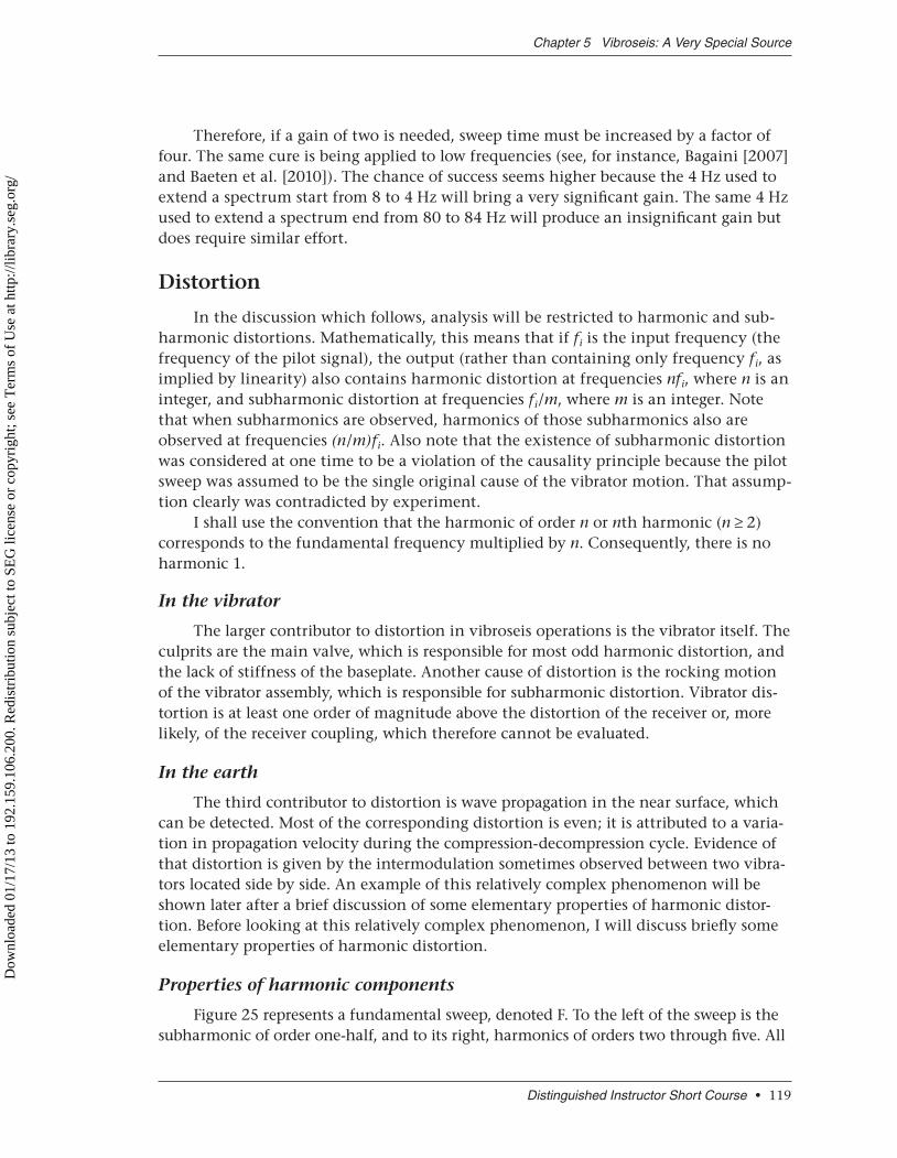
Figure 25 represents a fundamental sweep, denoted F. To the left of the sweep is the subharmonic of order one-half, and to its right, harmonics of orders two through five. All



Dow

nloa

ded

01/1

7/13

to 1

92.1

59.1

06.2

00. R

edis

trib

utio

n su

bjec

t to

SEG

lice

nse

or c

opyr

ight

; see

Ter

ms

of U

se a

t http

://lib

rary

.seg

.org

/

harmonics are represented with the same amplitude as the fundamental. In general, their amplitude is a frac-tion (one-tenth to one-fourth) of the fundamental amplitude.

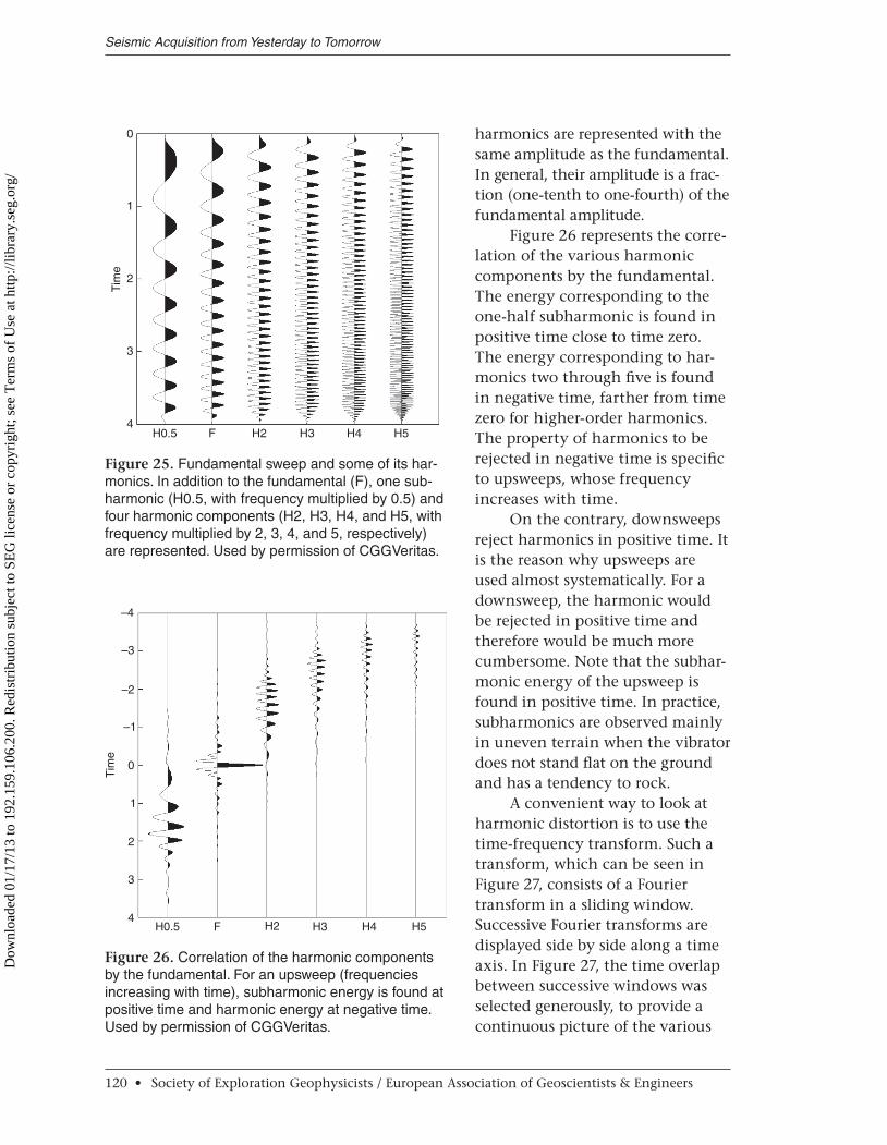
Figure 26 represents the corre-lation of the various harmonic components by the fundamental. The energy corresponding to the one-half subharmonic is found in positive time close to time zero. The energy corresponding to har-monics two through five is found in negative time, farther from time zero for higher-order harmonics. The property of harmonics to be rejected in negative time is specific to upsweeps, whose frequency increases with time.

On the contrary, downsweeps reject harmonics in positive time. It is the reason why upsweeps are used almost systematically. For a downsweep, the harmonic would be rejected in positive time and therefore would be much more cumbersome. Note that the subhar-monic energy of the upsweep is found in positive time. In practice, subharmonics are observed mainly in uneven terrain when the vibrator does not stand flat on the ground and has a tendency to rock.

A convenient way to look at harmonic distortion is to use the time-frequency transform. Such a transform, which can be seen in Figure 27, consists of a Fourier transform in a sliding window. Successive Fourier transforms are displayed side by side along a time axis. In Figure 27, the time overlap between successive windows was selected generously, to provide a continuous picture of the various



0

1

2

Tim

e

3

4H0.5 F H2 H3 H4 H5

Figure 25. Fundamental sweep and some of its har-monics. In addition to the fundamental (F), one sub-harmonic (H0.5, with frequency multiplied by 0.5) and four harmonic components (H2, H3, H4, and H5, with frequency multiplied by 2, 3, 4, and 5, respectively) are represented. Used by permission of CGGVeritas.

–4

–3

–2

–1

Tim

e

0

1

2

3

4H0.5 F H2 H3 H4 H5

Figure 26. Correlation of the harmonic components by the fundamental. For an upsweep (frequencies increasing with time), subharmonic energy is found at positive time and harmonic energy at negative time. Used by permission of CGGVeritas.

Dow

nloa

ded

01/1

7/13

to 1

92.1

59.1

06.2

00. R

edis

trib

utio

n su

bjec

t to

SEG

lice

nse

or c

opyr

ight

; see

Ter

ms

of U

se a

t http

://lib

rary

.seg

.org

/

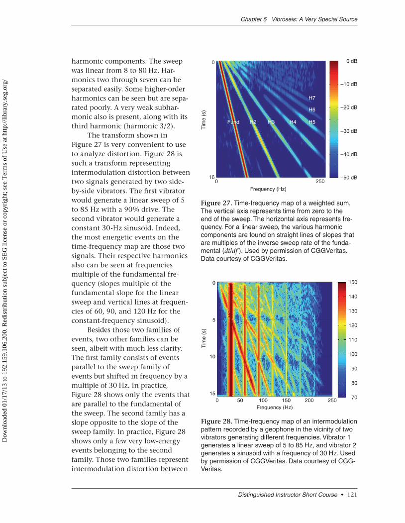
harmonic components. The sweep was linear from 8 to 80 Hz. Har-monics two through seven can be separated easily. Some higher-order harmonics can be seen but are sepa-rated poorly. A very weak subhar-monic also is present, along with its third harmonic (harmonic 3/2).

The transform shown in Figure 27 is very convenient to use to analyze distortion. Figure 28 is such a transform representing intermodulation distortion between two signals generated by two side-by-side vibrators. The first vibrator would generate a linear sweep of 5 to 85 Hz with a 90% drive. The second vibrator would generate a constant 30-Hz sinusoid. Indeed, the most energetic events on the time-frequency map are those two signals. Their respective harmonics also can be seen at frequencies multiple of the fundamental fre-quency (slopes multiple of the fundamental slope for the linear sweep and vertical lines at frequen-cies of 60, 90, and 120 Hz for the constant- frequency sinusoid).

Besides those two families of events, two other families can be seen, albeit with much less clarity. The first family consists of events parallel to the sweep family of events but shifted in frequency by a multiple of 30 Hz. In practice, Figure 28 shows only the events that are parallel to the fundamental of the sweep. The second family has a slope opposite to the slope of the sweep family. In practice, Figure 28 shows only a few very low-energy events belonging to the second family. Those two families represent intermodulation distortion between



0 0 dB

–10 dB

–20 dB

–30 dB

–40 dB

–50 dB

Tim

e (s

)

160 250

Frequency (Hz)

Fund H2 H3 H4 H5

H6

H7

Figure 27. Time-frequency map of a weighted sum. The vertical axis represents time from zero to the end of the sweep. The horizontal axis represents fre-quency. For a linear sweep, the various harmonic components are found on straight lines of slopes that are multiples of the inverse sweep rate of the funda-mental (dt/df ). Used by permission of CGGVeritas. Data courtesy of CGGVeritas.

0 150

140

130

120

110

100

90

80

70

5

10

Tim

e (s

)

150 50 100

Frequency (Hz)150 200 250

Figure 28. Time-frequency map of an intermodulation pattern recorded by a geophone in the vicinity of two vibrators generating different frequencies. Vibrator 1 generates a linear sweep of 5 to 85 Hz, and vibrator 2 generates a sinusoid with a frequency of 30 Hz. Used by permission of CGGVeritas. Data courtesy of CGG-Veritas.

Dow

nloa

ded

01/1

7/13

to 1

92.1

59.1

06.2

00. R

edis

trib

utio

n su

bjec

t to

SEG

lice

nse

or c

opyr

ight

; see

Ter

ms

of U

se a

t http

://lib

rary

.seg

.org

/

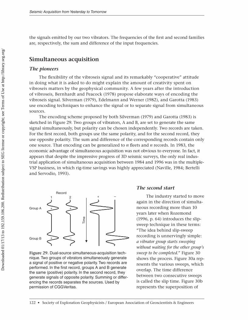
the signals emitted by our two vibrators. The frequencies of the first and second families are, respectively, the sum and difference of the input frequencies.

Simultaneous acquisition

The pioneers

The flexibility of the vibroseis signal and its remarkably “cooperative” attitude in doing what it is asked to do might explain the amount of creativity spent on vibroseis matters by the geophysical community. A few years after the introduction of vibroseis, Bernhardt and Peacock (1978) propose elaborate ways of encoding the vibroseis signal. Silverman (1979), Edelmann and Werner (1982), and Garotta (1983) use encoding techniques to enhance the signal or to separate signal from simultaneous sources.

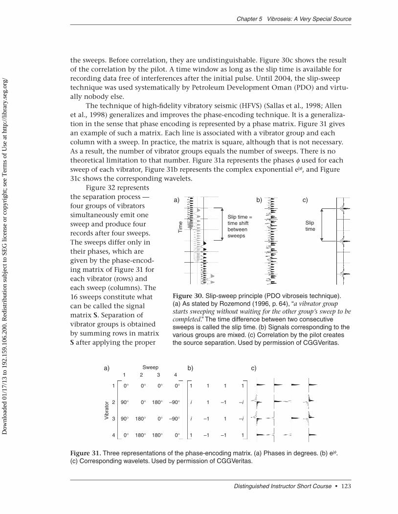
The encoding scheme proposed by both Silverman (1979) and Garotta (1983) is sketched in Figure 29. Two groups of vibrators, A and B, are set to generate the same signal simultaneously, but polarity can be chosen independently. Two records are taken. For the first record, both groups use the same polarity, and for the second record, they use opposite polarity. The sum and difference of the corresponding records contain only one source. That encoding can be generalized to n fleets and n records. In 1983, the economic advantage of simultaneous acquisition was not obvious to everyone. In fact, it appears that despite the impressive progress of 3D seismic surveys, the only real indus-trial application of simultaneous acquisition be tween 1984 and 1996 was in the multiple- VSP business, in which rig-time savings was highly appreciated (Naville, 1984; Bertelli and Servodio, 1993).

The second start

The industry started to move again in the direction of simulta-neous recording more than 10 years later when Rozemond (1996, p. 64) introduces the slip-sweep technique in these terms: “The idea behind slip-sweep recording is unnervingly simple: a vibrator group starts sweeping without waiting for the other group’s sweep to be completed.” Figure 30 shows the process. Figure 30a rep-resents the various sweeps, which overlap. The time difference between two consecutive sweeps is called the slip time. Figure 30b represents the superposition of



Record

Group A

Group B

1 2

Tim

e

+ +

+ –

+ –

Figure 29. Dual-source simultaneous-acquisition tech-nique. Two groups of vibrators simultaneously generate a signal of positive or negative polarity. Two records are performed. In the first record, groups A and B generate the same (positive) polarity. In the second record, they generate signals of opposite polarity. Summing or differ-encing the records separates the sources. Used by permission of CGGVeritas.

Dow

nloa

ded

01/1

7/13

to 1

92.1

59.1

06.2

00. R

edis

trib

utio

n su

bjec

t to

SEG

lice

nse

or c

opyr

ight

; see

Ter

ms

of U

se a

t http

://lib

rary

.seg

.org

/

the sweeps. Before correlation, they are undistinguishable. Figure 30c shows the result of the correlation by the pilot. A time window as long as the slip time is available for recording data free of interferences after the initial pulse. Until 2004, the slip-sweep technique was used systematically by Petroleum Development Oman (PDO) and virtu-ally nobody else.

The technique of high-fidelity vibratory seismic (HFVS) (Sallas et al., 1998; Allen et al., 1998) generalizes and improves the phase-encoding technique. It is a generaliza-tion in the sense that phase encoding is represented by a phase matrix. Figure 31 gives an example of such a matrix. Each line is associated with a vibrator group and each column with a sweep. In practice, the matrix is square, although that is not necessary. As a result, the number of vibrator groups equals the number of sweeps. There is no theoretical limitation to that number. Figure 31a represents the phases ϕ used for each sweep of each vibrator, Figure 31b represents the complex exponential ejϕ, and Figure 31c shows the corresponding wavelets.

Figure 32 represents the separation process — four groups of vibrators simultaneously emit one sweep and produce four records after four sweeps. The sweeps differ only in their phases, which are given by the phase-encod-ing matrix of Figure 31 for each vibrator (rows) and each sweep (columns). The 16 sweeps constitute what can be called the signal matrix S. Separation of vibrator groups is obtained by summing rows in matrix S after applying the proper



Slip time =time shiftbetweensweeps

a) b) c)

SliptimeT

ime

Figure 30. Slip-sweep principle (PDO vibroseis technique). (a) As stated by Rozemond (1996, p. 64), “a vibrator group starts sweeping without waiting for the other group’s sweep to be completed.” The time difference between two consecutive sweeps is called the slip time. (b) Signals corresponding to the various groups are mixed. (c) Correlation by the pilot creates the source separation. Used by permission of CGGVeritas.

Sweepa) b) c)1

1

2

Vib

rato

r

3

4

1

–1

1

–1

1

1

–1

–1

1

i

i

1

1

–i

–i

1

0∞

90∞

90∞

0∞

0∞

–90∞

–90∞

0∞

0∞

0∞

180∞

180∞

0∞

180∞

0∞

180∞

2 3 4

Figure 31. Three representations of the phase-encoding matrix. (a) Phases in degrees. (b) ejϕ. (c) Corresponding wavelets. Used by permission of CGGVeritas.

Dow

nloa

ded

01/1

7/13

to 1

92.1

59.1

06.2

00. R

edis

trib

utio

n su

bjec

t to

SEG

lice

nse

or c

opyr

ight

; see

Ter

ms

of U

se a

t http

://lib

rary

.seg

.org

/

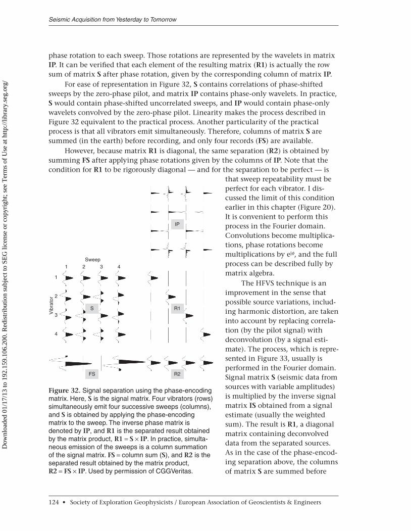
phase rotation to each sweep. Those rotations are represented by the wavelets in matrix IP. It can be verified that each element of the resulting matrix (R1) is actually the row sum of matrix S after phase rotation, given by the corresponding column of matrix IP.

For ease of representation in Figure 32, S contains correlations of phase-shifted sweeps by the zero-phase pilot, and matrix IP contains phase-only wavelets. In practice, S would contain phase-shifted uncorrelated sweeps, and IP would contain phase-only wavelets convolved by the zero-phase pilot. Linearity makes the process described in Figure 32 equivalent to the practical process. Another particularity of the practical process is that all vibrators emit simultaneously. Therefore, columns of matrix S are summed (in the earth) before recording, and only four records (FS) are available.

However, because matrix R1 is diagonal, the same separation (R2) is obtained by summing FS after applying phase rotations given by the columns of IP. Note that the condition for R1 to be rigorously diagonal — and for the separation to be perfect — is

that sweep repeatability must be perfect for each vibrator. I dis-cussed the limit of this condition earlier in this chapter (Figure 20). It is convenient to perform this process in the Fourier domain. Convolutions become multiplica-tions, phase rotations become multiplications by ejϕ, and the full process can be described fully by matrix algebra.

The HFVS technique is an improvement in the sense that possible source variations, includ-ing harmonic distortion, are taken into account by replacing correla-tion (by the pilot signal) with deconvolution (by a signal esti-mate). The process, which is repre-sented in Figure 33, usually is performed in the Fourier domain. Signal matrix S (seismic data from sources with variable amplitudes) is multiplied by the inverse signal matrix IS obtained from a signal estimate (usually the weighted sum). The result is R1, a diagonal matrix containing deconvolved data from the separated sources. As in the case of the phase-encod-ing separation above, the columns of matrix S are summed before



Sweep1

1

2

Vib

rato

r

3

4

2

S

FS R2

R1

IP

3 4

Figure 32. Signal separation using the phase-encoding matrix. Here, S is the signal matrix. Four vibrators (rows) simultaneously emit four successive sweeps (columns), and S is obtained by applying the phase-encoding matrix to the sweep. The inverse phase matrix is denoted by IP, and R1 is the separated result obtained by the matrix product, R1 = S × IP. In practice, simulta-neous emission of the sweeps is a column summation of the signal matrix. FS = column sum (S), and R2 is the separated result obtained by the matrix product, R2 = FS × IP. Used by permission of CGGVeritas.

Dow

nloa

ded

01/1

7/13

to 1

92.1

59.1

06.2

00. R

edis

trib

utio

n su

bjec

t to

SEG

lice

nse

or c

opyr

ight

; see

Ter

ms

of U

se a

t http

://lib

rary

.seg

.org

/

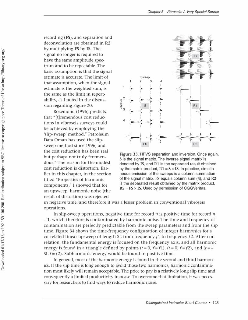
recording (FS), and separation and deconvolution are obtained in R2 by multiplying FS by IS. The signal no longer is required to have the same amplitude spec-trum and to be repeatable. The basic assumption is that the signal estimate is accurate. The limit of that assumption, when the signal estimate is the weighted sum, is the same as the limit in repeat-ability, as I noted in the discus-sion regarding Figure 20.

Rozemond (1996) predicts that “[t]remendous cost reduc-tions in vibroseis surveys could be achieved by employing the ‘slip-sweep’ method.” Petroleum Data Oman has used the slip-sweep method since 1996, and the cost reduction has been real but perhaps not truly “tremen-dous.” The reason for the modest cost reduction is distortion. Ear-lier in this chapter, in the section titled “Properties of harmonic components,” I showed that for an upsweep, harmonic noise (the result of distortion) was rejected in negative time, and therefore it was a lesser problem in conventional vibroseis operations.

In slip-sweep operations, negative time for record n is positive time for record n – 1, which therefore is contaminated by harmonic noise. The time and frequency of contamination are perfectly predictable from the sweep parameters and from the slip time. Figure 34 shows the time-frequency configuration of integer harmonics for a correlated linear upsweep of length SL from frequency f1 to frequency f2. After cor-relation, the fundamental energy is focused on the frequency axis, and all harmonic energy is found in a triangle defined by points (t = 0, f = f1), (t = 0, f = f2), and (t = – SL f = f2). Subharmonic energy would be found in positive time.

In general, most of the harmonic energy is found in the second and third harmon-ics. If the slip time is long enough to avoid those two harmonics, harmonic contamina-tion most likely will remain ac ceptable. The price to pay is a relatively long slip time and consequently a limited productivity increase. To overcome that limitation, it was neces-sary for researchers to find ways to reduce harmonic noise.



Sweep1

1

2

S

FS R2

R1

IS

Vib

rato

r

3

4

2 3 4

Figure 33. HFVS separation and inversion. Once again, S is the signal matrix. The inverse signal matrix is denoted by IS, and R1 is the separated result obtained by the matrix product, R1 = S × IS. In practice, simulta-neous emission of the sweeps is a column summation of the signal matrix. FS equals column sum (S), and R2 is the separated result obtained by the matrix product, R2 = FS × IS. Used by permission of CGGVeritas.

Dow

nloa

ded

01/1

7/13

to 1

92.1

59.1

06.2

00. R

edis

trib

utio

n su

bjec

t to

SEG

lice

nse

or c

opyr

ight

; see

Ter

ms

of U

se a

t http

://lib

rary

.seg

.org

/

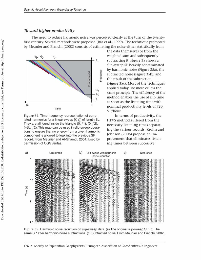
Toward higher productivity

The need to reduce harmonic noise was perceived clearly at the turn of the twenty-first century. Several methods were proposed (Ras et al., 1999). The technique promoted by Meunier and Bianchi (2002) consists of estimating the noise either statistically from

the data themselves or from the weighted sum and subsequently subtracting it. Figure 35 shows a slip-sweep SP heavily contaminated by harmonic noise (Figure 35a), the subtracted noise (Figure 35b), and the result of the subtraction (Figure 35c). Most of the techniques applied today use more or less the same principle. The efficiency of the method enables the use of slip time as short as the listening time with nominal productivity levels of 720 VP/hour.

In terms of productivity, the HFVS method suffered from the necessary listening times separat-ing the various records. Krohn and Johnson (2006) propose an im-prove ment that eliminates listen-ing times between successive



H4 H3 H2

–SL 0

f2

3f12f1

f1

Fun

dam

enta

l

Freq

uenc

y

Time

Figure 34. Time-frequency representation of corre-lated harmonics for a linear sweep [f1 f2] of length SL. They are all found inside the triangle (0, f1), (0, f 2), (–SL, f2). This map can be used in slip-sweep opera-tions to ensure that no energy from a given harmonic component is allowed to leak into the previous SP record. From Meunier and Al-Ghamdi, 2004. Used by permission of CGGVeritas.

Slip sweep

0

0.5

Tim

e (s

)

1

1.5

a) b) c)Slip sweep with harmonicnoise reduction

Difference

Figure 35. Harmonic noise reduction on slip-sweep data. (a) The original slip-sweep SP. (b) The same SP after harmonic-noise subtractions. (c) Subtracted noise. From Meunier and Bianchi, 2002.

Dow

nloa

ded

01/1

7/13

to 1

92.1

59.1

06.2

00. R

edis

trib

utio

n su

bjec

t to

SEG

lice

nse

or c

opyr

ight

; see

Ter

ms

of U

se a

t http

://lib

rary

.seg

.org

/

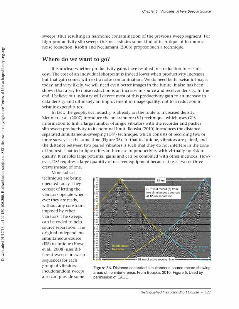
sweeps, thus resulting in harmonic contamination of the previous sweep segment. For high-productivity slip sweep, this necessitates some kind of technique of harmonic noise reduction. Krohn and Neelamani (2008) propose such a technique.

Where do we want to go?

It is unclear whether productivity gains have resulted in a reduction in seismic cost. The cost of an individual shotpoint is indeed lower when productivity increases, but that gain comes with extra noise contamination. We do need better seismic images today, and very likely, we will need even better images in the future. It also has been shown that a key to noise reduction is an increase in source and receiver density. In the end, I believe our industry will devote most of this productivity gain to an increase in data density and ultimately an improvement in image quality, not to a reduction in seismic expenditures.

In fact, the geophysics industry is already on the route to increased density. Meunier et al. (2007) introduce the one-vibrator (V1) technique, which uses GPS information to link a large number of single vibrators with the recorder and pushes slip-sweep productivity to its nominal limit. Bouska (2010) introduces the distance- separated simultaneous-sweeping (DS3) technique, which consists of recording two or more surveys at the same time (Figure 36). In that technique, vibrators are paired, and the distance between two paired vibrators is such that they do not interfere in the zone of interest. That technique offers an increase in productivity with virtually no risk to quality. It enables large potential gains and can be combined with other methods. How-ever, DS3 requires a large quantity of receiver equipment because it uses two or three crews instead of one.

More radical techniques are being operated today. They consist of letting the vibrators operate when-ever they are ready, without any constraint imposed by other vibrators. The sweeps can be coded to help source separation. The original independent- simultaneous-source (ISS) technique (Howe et al., 2008) uses dif-ferent sweeps or sweep sequences for each group of vibrators. Pseudorandom sweeps also can provide some



12 km

Interference-free zone

18 km of active receiver line

Interference-free zone

0.000.100.200.300.400.500.600.700.800.901.001.101.201.301.401.501.601.701.801.902.002.102.202.302.40

2.602.702.802.903.003.103.203.303.403.50

2.50

DS3 field record (s) from two simultaneous sources at 12-km separation

Figure 36. Distance-separated simultaneous-source record showing areas of noninterference. From Bouska, 2010, Figure 5. Used by permission of EAGE.

Dow

nloa

ded

01/1

7/13

to 1

92.1

59.1

06.2

00. R

edis

trib

utio

n su

bjec

t to

SEG

lice

nse

or c

opyr

ight

; see

Ter

ms

of U

se a

t http

://lib

rary

.seg

.org

/

initial source separation. Using that technique, Pecholcs et al. (2010) report a productiv-ity of 45,501 SP per day. Alternatively, the sweeps all might be strictly identical. Then it would be necessary to operate source separation at the processing stage.

Conclusion

The route is opened. It is very likely that traffic will increase despite the many obstacles that already can be identified (such as environmental concerns, organization, processing, and cost) and those that still hide along the way.



Dow

nloa

ded

01/1

7/13

to 1

92.1

59.1

06.2

00. R

edis

trib

utio

n su

bjec

t to

SEG

lice

nse

or c

opyr

ight

; see

Ter

ms

of U

se a

t http

://lib

rary

.seg

.org

/

Documents

5. Chapter 5 Vibroseis- A Very Special Source