5 Photo-Point Monitoring - US EPA · Monitoring and Evaluating Nonpoint Source Watershed Projects Chapter 5 . 5-1 . 5 Photo-Point Monitoring . ... trash removal and ... and they are

Monitoring and Evaluating Nonpoint Source Watershed Projects Chapter 5

5-1

5 Photo-Point Monitoring By S.A. Dressing and D.W. Meals

5.1 Introduction Good photographs can yield much information, and photography can play important roles in watershed projects because the technology is available to everyone, training is simple, and the cost is relatively low (USEPA 2008, ERS 2010). In the assessment phase, photos can help identify problem areas both within the water resource (e.g., algal blooms, streambank erosion) and within the drainage area (e.g., cattle in streams, discharge pipes). These same photos can also be very helpful in generating interest in the project because they can convey easily understood information to a wide audience. In addition, photos can be used to document implementation of practices including contour strip-cropping, stream buffers, rain gardens, and other practices where physical changes are observable. Finally, photos can be used in project evaluation. For example, photos taken before and after implementation of some types of remedial efforts (e.g., trash removal and prevention) provide an indicator of progress that can be communicated easily to most people.

To be useful, however, photographs must be taken in accordance with a protocol that ensures the photographic database accurately represents watershed conditions and is suitable for meeting stated objectives. This section provides an overview of ground-based photographic, or photo-point, monitoring, including specific elements of an acceptable protocol and example applications.

5.2 Procedure Photo-point monitoring requires careful planning to ensure that meaningful information is provided to assess condition or trends (Bauer and Burton 1993). Monitoring design begins with a set of clear objectives, and different objectives will generally require different photo points (Hamilton, n.d.).

There are two basic methods of photo-point monitoring – comparison photography and repeat photography – but these methods can be used in combination (i.e., comparison photography repeated over time). Method selection should generally precede other design decisions but choices made in one step of monitoring plan design can affect the options in other steps, so flexibility is necessary. Selection of monitoring areas, identification of the specific features to photograph, camera placement, and the timing and frequency of photography are all typically determined after monitoring objectives and basic method are addressed (after Hamilton n.d.).

Photo-Point Monitoring • Set objectives • Select method • Select monitoring areas • Establish, mark, and assign

identification numbers to photo and camera points

• Identify a witness site • Record site information and create a

site locator field book • Determine timing and frequency of

photographs • Define data analysis plans • Establish data management system • Take and document photos


5-2

All photo and camera locations must be marked, monitoring site characteristics must be recorded, and a field book or similar documentation should be created to assist those taking photographs at the sites over time. This is critical if different people will be taking photographs throughout the course of a project. Plans for analysis of the photos and use of any photo-derived information must be determined and documented before photo-point monitoring begins. The data analysis plan will also help determine how best to organize and file photos and metadata.

These various design steps are described in greater detail below.

5.2.1 Setting Objectives There will most likely be different photo-point monitoring objectives for project assessment, planning, implementation, and evaluation. Objectives for all project phases should be defined as early on in the project as possible, however, to maximize the efficiency of the photo-point monitoring effort. It may be possible, for example, to use photos from problem assessment or planning as pre-implementation photos for tracking implementation.

Realistic objectives begin with an understanding of what is likely to be seen and measured with photographs. Cameras exist that can take photos in both the visible and the non-visible spectrum (e.g., infrared or ultraviolet). For example, aerial photography has been used successfully to identify sediment sources at the watershed scale through correlation of photo density readings from the transparencies of color-infrared photographs with suspended sediment measurements (Rosgen 1973 1976). In addition, Hively et al. (2009a 2009b) combined cost-share program enrollment data with satellite imagery and on-farm sampling to evaluate cover crop N uptake on 136 fields within the Choptank River watershed on Maryland’s eastern shore. Thermal infrared (TIR) images acquired from airborne platforms have been used in stream temperature monitoring and analysis programs, detecting and quantifying warm and cool water sources, calibrating stream temperature models, and identifying thermal processes (Faux et al. 2001). TIR imagery has also been used in the mapping of groundwater inflows and the analysis of floodplain hydrology. While such applications are indeed useful, this guidance and the example objectives that follow focus solely on ground-based photography in the visible spectrum.

An array of observable features listed in various guidance documents includes pasture condition, livestock distribution in a meadow, ground cover, tree canopy and health, vegetation density, woody vegetation, native vegetation area, wetland area, native plant richness, large trees, stream profile, streambank stability, streambank cover, fallen woody material and in-stream habitat, farm water flow, gully erosion, hill slope erosion, wind erosion, weed cover and species (Bauer and Burton 1993, ERS 2010, Hall 2001, Shaff et al. 2007). In addition, Hall (2001) provides numerous examples of successes and failures to measure changes in observable features with photo-point monitoring.

Examples of potential objectives for photo-point monitoring at various project stages include the following.

Assessment

Document trash levels on beaches or in urban settings

Document stream features

Document algal blooms in waterbodies

Identify sources of sediment plumes


5-3

Document livestock activity near waterbodies

Identify gullies and areas of streambank instability

Identify areas in greatest need of urban runoff control measures

Planning

Help locate areas were streambank protection and stream restoration are needed

Document livestock operation needs to assist in budget development

Provide evidence of watershed problems and potential solutions for public outreach

Provide photos to assist the design of urban runoff control measures

Implementation

Document tree growth in riparian zone over time

Document implementation of rain gardens

Document stream restoration activities

Document and track changes in percent residue at representative agricultural sites across a watershed

Evaluation

Document changes in streambank cover or stream profile as a result of stream restoration

Demonstrate the effects of different grazing management systems on pasture condition

Illustrate how a stream handles high-flow events before and after restoration

Document changes in beach trash over time

The type and rigor of photo-point monitoring needed to meet these objectives varies. Alternative methods are described below.

5.2.2 Selecting Methods As defined by Hall (2001), ground-based photo monitoring involves “using photographs taken at a specific site to monitor conditions or change,” something that is accomplished by one of two methods: comparison or repeat photography. Comparison photography typically involves the creation of a photo guide from a set of standard photos taken to represent the expected range of an attribute (or condition) of interest (e.g., utilization of grazing plants). Field measurements are taken to establish values for the attribute of interest at levels represented by each of the photos in the guide. Figure 5-1 illustrates the concept whereby the value (percentage of area covered with dots) is determined from field measurement of the attribute of interest (dots/unit area in this conceptual example). The comparison photos in the guide are then used in the field to perform on-site assessment.


5-4

Photo 1 Photo 2 Photo 3 Photo 4 Photo 5

Value 5%

Value 10%

Value 20%

Value 30%

Value 40%

Figure 5-1. Comparison photos

In repeat photography, photos are taken of the subject over time at the same location to document change or monitor activity. Repeat photography has been used to document landscape change, including the advance and retreat of glaciers (Key et al. 2002). This method has also been used extensively to document progress in dam removal (USDA-FS 2007), riparian area protection (Bauer and Burton 1993), and stream restoration projects (Bledsoe and Meyer 2005).

A third type of photography is opportunistic photography. As described by Shaff et al. (2007), opportunistic photos are not taken from a permanently marked location, and they are not part of a repeat photography effort. There is also no photo guide as is used in comparison photography. Examples of subjects that can be addressed with opportunistic photography include a site during construction or an area after a significant natural or human-induced event.

Comparison photography is generally well suited to meeting assessment objectives in cases where photography is an appropriate monitoring approach. Opportunistic photography also usually plays a role in problem assessment. Both methods can be used for qualitative purposes, and comparison photography can be used in quantitative analyses to a limited degree (see “Qualitative” and “Quantitative” below). Opportunistic photography is not designed for quantitative analyses, however. Other information sources (e.g., livestock inventories, street maps, and permitted discharge reports) and monitoring data (e.g., water chemistry, aquatic biology, and habitat) will be needed in combination with photos to meet assessment objectives.

A combination of comparison and opportunistic photography can be helpful in achieving planning objectives, coupled with information from other sources. Opportunistic photos, in particular, can be quite helpful in communicating to the general public and stakeholders the need for restoration or BMPs to achieve watershed objectives. Visual inventories can be helpful in estimating implementation costs but should be used in combination with more traditional approaches to assessing need.


5-5

Repeat photography is generally most useful for tracking restoration and implementation of BMPs. Comparison photos can be used to assess such important indicators as the extent that conservation tillage has resulted in increased percent residue. Opportunistic photos can help show how restored stream reaches or urban runoff practices handle high-flow events.

While photo-point monitoring can be very helpful, it should be kept in mind that tracking implementation of rain gardens, for example, does not require photos. Observers could simply record in a database that a rain garden has been implemented at a specific address or global positioning system (GPS) location, but a photograph might add valuable information about the rain garden (e.g., size, location, plant selection and density) that could be explored at a later date if water quality data raise questions about rain garden performance.

Watershed projects cannot rely on photographs as the sole source of information for problem assessment or planning. Project implementation is nearly always tracked by means other than photo-point monitoring, but the addition of photographs can be the best way to document the installation of structural practices (e.g., lagoons, constructed wetlands) or the growth of vegetation associated with stream restoration or grazing management. It is important to keep in mind that photo-point monitoring should always be considered as a cost-effective tool for providing information in conjunction with other monitoring and information gathering efforts. While there are examples where photo-point monitoring is relied on as the primary monitoring method due to budgetary constraints, it is not recommended.

All three photo-point monitoring methods – comparison, repeat, and opportunistic – can support qualitative analyses, and comparison and repeat photography can also be used in quantitative analyses.

5.2.2.1 Qualitative Monitoring Photographic monitoring methods usually generate qualitative information (e.g., Shaff et al. 2007). Creating a pictorial record of changing conditions, showing major changes in shrub and tree populations, visually representing physical measurements taken at a location, or recording particular events such as floods are typical of the types of photo-point monitoring objectives stated for these projects (ERS 2010). Those who have used photographic monitoring for watershed projects have generally used this method to document implementation of practices, typically the growth of vegetation associated with stream/streambank restoration or grazing management. These qualitative findings have been used most frequently to corroborate findings from more quantitative monitoring methods.

Photos are recommended for long-term monitoring of grassland, shrubland, and savanna ecosystems but simply as a qualitative indicator of large changes in vegetation structure and for visually documenting changes measured with other methods (Herrick et al. 2005 2005a). Photos should not be considered as a substitute for quantitative data; it is very difficult to obtain reliable quantitative data from photos unless conditions are controlled. Bledsoe and Meyer (2005) used photographs to compare changes from year to year, document noteworthy morphologic adjustments, document features of interest at various locations and times during the year, and analyze vegetation establishments as part of monitoring channel stability.

5.2.2.2 Quantitative Monitoring Quantitative monitoring involves either measurement or counting. When measurement is desired it is important to use meter boards (field rulers mounted vertically) or other size control boards to provide a reference for measurement (Hall 2001 2002). Small frames (1 m2) have been used for closeup or plot studies, while meter boards and Robel poles are often used for more distant studies. These standard


5-6

references are captured within the photographs to provide a means of measuring features of interest. Counts of items of interest (e.g., trees of varying heights) can be obtained through visual observation of images. Another alternative for obtaining counts or percentages for quantitative analysis is to count digital image pixels that fall within a specified color range (see Digital Image Analysis below).

Meter boards can also provide a consistent point for camera orientation and a point on which to focus the camera (Hamilton n.d.). Figure 5-2 illustrates the use of a meter board and photo identification card (see section 5.2.13). The following are methods described by Hall (2001) that incorporate varying degrees of quantitative analysis. It should be noted that while these methods all support some level of quantification, documentation of precision and accuracy is generally lacking.

Figure 5-2. Illustration of a photo identification card and a meter board

5.2.2.2.1 Photo Grid Analysis Photo grid analysis involves placing a standardized grid over a photo and counting the number of intersects between the grid lines and features of interest. When photo grid analysis is planned, it is very important that the distance between the camera and meter board is constant (Hall 2001 2002). It is recommended that the camera height is held constant, but it is only required to be constant if the grid is used to track position (in addition to size) of features over time. The size control board should cover at least 25 percent of the photo height, with the optimum range being 35 to 50 percent. The board, however,


5-7

cannot obstruct the features of interest that will be measured. A level meter control board is preferred because it will match up more easily with a superimposed grid. Vegetation around the front of the meter board should be removed to expose the bottom measurement line to provide maximum precision in grid adjustment.

Hall (2001 2002) notes that both grid precision and observer variability are major factors in determining the ability to measure change. The percentage of photo height taken by the meter board is a very important factor in the precision with which grids are fit. It should be noted that changes in technology (cameras and software) may provide better results than found by Hall. For example, testing showed that a meter board that covers 35 percent of the photo height was 1.3 times more precise than a board that covered 25 percent of the photo height. Testing on observer variability also indicated that, on average, a change >12 percent in intersects for all shrubs (a measurement for grid analysis) was needed to demonstrate change at the 5 percent confidence level. Additional details and examples of photo grid analysis are provided by Hall (2001 2002).

5.2.2.2.2 Transect Photo Sampling Photo points can also be established along a transect to obtain more quantitative information (Hamilton n.d.). Hall (2001) describes in detail five kinds of photo transects: (1) 1-ft2 frequency photographed with or without a stereo attachment on the camera, (2) nested frequency using four plot sizes in a 0.5- by 0.5-m frame, (3) 1-m2 plot frame photographed at an angle, (4) vertical photographs of tree canopy cover, and (5) measurement of herbaceous stubble height using the Robel pole system.

Transect installation is straightforward, requiring skillsets and procedures similar to those for the establishment of photo-point and camera sites (see sections 5.2.4 and 5.2.5). Equipment needs are similar as well. Size control boards are required, and they can serve multiple purposes, including estimation of height of grass and shrubs, orientation (for consistency) and focus (for greatest depth of field) of the camera, and grid analysis (Hall 2001). Key features of the five kinds of photo transects are provided below, but the reader should not select any of these methods until reviewing the detailed discussion of each by Hall.

5.2.2.2.2.1 One-Square-Foot Sampling This method uses a 1-ft2 plot placed every 5 ft along a 100-ft transect. The 20 plots are monitored to document changes in species, species density, and frequency as a means to estimate change in vegetation and soil surface conditions. Statistical analysis of data generated by this method is not possible.

5.2.2.2.2.2 Nested Frequency This method uses a sample frame with four nested plot sizes to document change in species frequency along five 100-ft transects of 20 plots each. Statistical analysis suggests significant change in frequency (the number of times a species occurs in a given number of plots) at the 80-percent level of probability.

5.2.2.2.2.3 Nine-Square-Foot Transects This plot system uses five 9-ft2 plots along a 100-ft transect to document changes in species frequency. Photographs are taken of the plot frame at an oblique angle rather than from directly above. Interpretation of change is based not on statistical analysis but on professional judgment and interpretation of the photos.


5-8

5.2.2.2.2.4 Tree Canopy It is recommended that any transect placed in a forest setting should have tree cover sampled because of its effects on the density and composition of ground vegetation. Tree canopies are photographed from ground level by using a camera leveling board or other means to ensure that the camera is pointing directly above. The method requires photographs of tree cover at the 0-, 25-, 50-, 75-, and 100-ft locations on transects used for any of the three methods described above. Because photo grid analysis is used to estimate tree cover, the same focal length must be used for all photos and the long axis of the camera should be perpendicular to the transect.

5.2.2.2.2.5 Robel Pole A Robel pole is a 4-ft pole with 1-in bands painted in alternating colors (USDA-CES et al. 1999). Vegetation height is measured by photographing the pole from a specific distance and height above the ground. This is accomplished by attaching a 4-m-long line between the 1-m mark on the Robel pole and the top of a 1-m-tall line pole. The Robel pole is placed at the sample location and the line is stretched out. The camera is set on top of the line pole and a photo is taken. By consistently using the 4-m line and 1-m camera height (4-to-1 ratio), the same angle is obtained for all photos.

5.2.2.2.3 Digital Image Analysis Many of the methods described by Hall (2001) were centered on film-based photography, and they often require a substantial amount of measurement and analysis by hand. Newer methods such as digital image analysis (DIA) use computers to analyze digital images, offering the potential advantages of improved objectivity, accuracy, and precision. In one form of DIA, color images are converted to grayscale (monochrome) images using an algorithm that converts each pixel to white or black based on the color content of the original pixel. The algorithm in this case is designed to select those colors that represent the feature to be counted. For example, Rasmussen et al. (2007) used DIA to determine the proportion of pixels in digital images that were green to estimate crop soil cover in weed harrowing research.

There are significant hurdles to overcome in applying DIA to photo-point monitoring for watershed projects. Factors such as lighting, camera angle, size of the area photographed, and the growth stage of plants should be evaluated to quantify their effects on the accuracy or precision of the method (Rasmussen et al. 2007). It is also important to have a true value to compare against the DIA-based results to assess the accuracy of the method (Richardson et al. 2001).

A significant contribution to DIA made by Rasmussen et al. (2007) was automated determination of the gray-level threshold which defines the difference between vegetation (the subject of interest in their study) and non-vegetation. This is especially important when lighting conditions vary in the field. With this capability, the researchers were able to develop an automated DIA procedure for converting each digital image into a single leaf cover (proportion of pixels that are green) value for analysis. Their research used the MATLAB Image Processing Toolbox (MathWorks 2012) but other options include Mathematica (Wolfram 2012) and a wide range of image processing products developed for a large number of applications.


5-9

5.2.3 Selecting Areas to Monitor The areas selected for photo-point monitoring must be appropriate for the stated objectives and consistent with the data analysis plans (section 5.2.11). Depending on the monitoring objectives, suitable sampling locations may be chosen to represent average or extreme conditions.

For problem assessment where opportunistic photography is used, site selection may be similar to that employed in a synoptic survey for water quality monitoring. Photos may be taken by individuals walking the stream to identify areas of streambank erosion or point source discharges. Photography of sources could involve a windshield-survey approach where photos are taken on a pre-determined route. Each opportunistic photo would need to be properly labeled as described in section 5.2.13.

When tracking project implementation (e.g., BMPs, restoration) or evaluating project success, it is most important to select an area that is most likely to undergo the physical transformations that can and must be tracked in order to support these objectives. Hall (2001) notes that this task may be straightforward (e.g., measuring the impact of stream restoration on the segment restored) or somewhat more complicated (e.g., documenting the impacts of livestock grazing on riparian vegetation). The latter case is more complicated because it requires some knowledge of livestock distribution, areas sensitive to grazing, and grazing patterns. Because it is likely that only a portion of the area of interest can be monitored, it is important to determine up front whether or not the findings can be extrapolated to areas not monitored. This is particularly challenging for photo-point monitoring because statistical analysis of photo-based data is not common. Attribution of sample findings to the broader area of interest would require the sample is representative, there is a measurable variable from the photos, the distribution for that variable is known, and an estimate of the standard deviation is available.

Some may wish to use photo-point monitoring to track BMP-related information in support of a traditional biological or chemical monitoring program. For example, if total suspended sediment concentration or loads are monitored in a predominantly agricultural watershed, it may be useful to track percent residue as an indicator of the extent to which reduced tillage practices have been implemented across the watershed. This could be accomplished in a number of ways including photo-point monitoring of a set of randomly selected field sites. Both comparison (to determine percent residue) and repeat (to track changes in percent residue over time) photography would be used in this application (see section 5.2.2). Again, attribution of sample findings to the broader area would require that the samples are representative, the distribution of percent residue is known, and an estimate of the standard deviation is available.

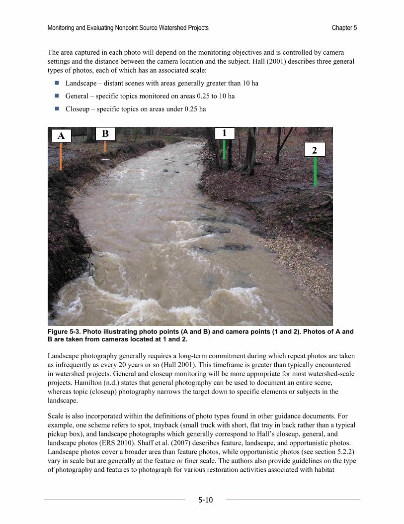
5.2.4 Identifying Photo Points Photo points are defined somewhat differently in various guidance manuals, which can lead to confusion when flipping back and forth between manuals. This document adopts the terminology used by Hall (2001), in which the photo point is essentially what you point the camera at when you take the photograph, and the camera point is a permanently marked location for the camera (Figure 5-3). Photo points have also been defined as permanent or semi-permanent sites set up from where you take a series of photographs over time (ERS 2010). Despite the different definitions and intermingling of various concepts within these definitions, photo-point monitoring manuals ultimately address the area to be photographed, the location from which the photos are taken, and the camera direction and settings to identify what will be captured in the photos. In simple terms, the photo point is what you point the camera at when you take the photograph.


5-10

The area captured in each photo will depend on the monitoring objectives and is controlled by camera settings and the distance between the camera location and the subject. Hall (2001) describes three general types of photos, each of which has an associated scale:

Landscape – distant scenes with areas generally greater than 10 ha

General – specific topics monitored on areas 0.25 to 10 ha

Closeup – specific topics on areas under 0.25 ha

Figure 5-3. Photo illustrating photo points (A and B) and camera points (1 and 2). Photos of A and B are taken from cameras located at 1 and 2.

Landscape photography generally requires a long-term commitment during which repeat photos are taken as infrequently as every 20 years or so (Hall 2001). This timeframe is greater than typically encountered in watershed projects. General and closeup monitoring will be more appropriate for most watershed-scale projects. Hamilton (n.d.) states that general photography can be used to document an entire scene, whereas topic (closeup) photography narrows the target down to specific elements or subjects in the landscape.

Scale is also incorporated within the definitions of photo types found in other guidance documents. For example, one scheme refers to spot, trayback (small truck with short, flat tray in back rather than a typical pickup box), and landscape photographs which generally correspond to Hall’s closeup, general, and landscape photos (ERS 2010). Shaff et al. (2007) describes feature, landscape, and opportunistic photos. Landscape photos cover a broader area than feature photos, while opportunistic photos (see section 5.2.2) vary in scale but are generally at the feature or finer scale. The authors also provide guidelines on the type of photography and features to photograph for various restoration activities associated with habitat


5-11

improvement projects, road projects, water management projects, wetlands, and fish passage improvement.

Be sure to consider the following when establishing photo points:

The general or specific features that must be photographed to meet the monitoring objectives.

How representative the photo points are of conditions in the study area.

Whether the number and type of photo points are sufficient for tracking change.

Whether changes will be visible at the desired scale.

Whether the site is accessible and lighting and sight lines are adequate during the entire monitoring period.

5.2.5 Establishing Camera Points As noted in section 5.2.4, camera points are permanently marked locations for the camera. Hamilton (n.d.) suggests selecting camera points from which multiple photo points can be photographed. The same photo point can also be photographed from multiple camera points, for example, if there is a need to examine the subject matter at different scales or from different angles. If the sizes of objects will be compared in photos taken from multiple camera points, the distance from each camera point to the photo point must be the same. In addition, to avoid shadowing of the photo point, camera points should be located north of photo points when they are close together.

Hall (2001) performed field testing of camera point setups (e.g., distance from photo point and the vertical and horizontal positioning of the camera) to determine the effects of various camera positions and settings on the ability to perform reliable repeat photography. Results of this testing clearly showed the following:

Distance from the camera to the meter board (or subject) affects both the size and location of objects photographed.

The vertical and horizontal position of the camera affects the location but not the size of objects photographed.

Focal length is not a critical issue because images can be enlarged or reduced to a constant area of coverage. Resolution can be lost, however, if images are enlarged or cropped too much, so it is best that the same or similar focal length be used for all photos.

Depending on the study objectives, therefore, camera point setup should provide a constant distance from the camera to the photo point (for size and location considerations), and consistent height and left-right orientation of the camera (for location). It should be noted that in Hall’s testing, camera position was shifted both upward and sideways by 40 cm (16 in) from an initial position centered at 1.4 m (55 in) above the ground. Smaller shifts would result in lesser changes in object location.

Figure 5-3 illustrates the location of photo and camera points. Both camera points 1 and 2 would need consistent camera positions if object locations were to be tracked over time. Meter boards can be used to guide camera position when taking photos, with the camera siting always on the top, bottom, or other specific marking on the meter board.


5-12

A recommended standard equipment list for establishing photo-point monitoring areas can be found in section 5.3.

5.2.6 Marking and Identifying Photo and Camera Points Every photo and camera point should be geolocated, photographed, and permanently marked so that those returning to take photos can find the sites with little waste of time. Capturing prominent features such as a ridge line in the photos can help others identify the location and the photo points (Bauer and Burton 1993). Labor is usually the greatest cost associated with monitoring efforts (see chapter 9), and doing whatever it takes to minimize the time needed to find photo-monitoring sites is cost effective. If volunteers perform the monitoring, marking of photo and camera points is essential to efficiently finding the locations so they can spend more time taking and documenting photos and less time searching for sites.

The best material to mark sites depends on the circumstances, but metal fenceposts work well in many cases (Hamilton n.d.). If metal fenceposts are unsuitable due to appearance or other considerations, steel survey stakes driven into the ground may be appropriate provided that metal detecting equipment is available (Hall 2001). If steel stakes are used, they can be covered with plastic pipe for safety, and all stakes can be painted in bright colors to improve visibility (Larsen 2006). Each photo and camera point should be given a unique identification number.

It is very important that the distance between camera points and photo points is measured and documented (Hamilton n.d.). Site location can be facilitated by use of a GPS but marking of photo and camera points will still be necessary in many cases, given that the best resolution for GPS systems is currently about 3-5 meters. Identifiers for opportunistic photos and temporary photo and camera points used for problem assessment and planning should at least include the purpose, address or GPS coordinates, camera direction, date photos were taken, narrative description of what was observed, and photographer name to provide sufficient information to interpret the information obtained and revisit the site if necessary.

5.2.7 Identifying a Witness Site A witness site is an object that can be easily identified when returning to the monitoring area (Hamilton n.d., Hall 2001). It may be a large rock, a structure, or other feature that is easily identifiable from the road or path to the photo and camera points. It is important to measure and document the distance and direction from the witness site to the camera points, photo points, or both. If possible, it is also helpful to attach a permanent identification tag to the witness site with the distance and direction to the photo and/or camera points inscribed on the tag (Hamilton n.d.). Newer photo-monitoring guidance recommends the use of GPS devices to facilitate finding the photo and camera points (ERS 2010, Shaff et al. 2007). In all cases, however, it is helpful to have photographs of the site and a description of landmarks to help locate and identify important spots within the monitoring area.

5.2.8 Recording Important Site Information Information about any monitoring site, whether it be chemical, biological, physical, or photographic (permanent or temporary), should be recorded to help future staff understand the reasons for selecting the site and to help in the interpretation of data collected from the site. Maps, aerial photographs, and


5-13

standardized forms can be used to record date, observer name(s), location, site description, objectives, identification numbers, and locations of the witness site, photo points, and camera points, including distances and directions between points. It is important to indicate whether directions are magnetic or true degrees (Hamilton n.d.), a topic addressed in detail by the U.S. Search and Rescue Task Force (USSARTF n.d.). Standardized forms for all aspects of photo-point monitoring can be found in existing documents (Hall 2001 2002, Shaff et al. 2007).

5.2.9 Determining Timing and Frequency of Photographs Monitoring frequency should be based primarily on the monitoring objectives, planned data analyses, features to be photographed, and expectations regarding detectable change in those features. Photo-point monitoring for problem assessment and planning can be a one-time activity or may involve multiple photographs taken at various times during the year to characterize seasonal, flow-related, or other significant variability. Efforts to track project implementation or evaluate project success will usually involve multiple years, with the frequency and timing of photos based on an understanding of seasonal and other variability.

Land managers are encouraged to photograph native vegetation at least once per year at the end of the growing season, or twice per year to show seasonal differences (ERS 2010). For restoration projects, the frequency options are generally seasonal, annual, or biennial (Shaff et al. 2007). In addition, photos taken during the high-flow and low-flow seasons should be compared to give some indication of the causes affecting streambank condition. Regardless of the frequency selected, annual changes should be assessed using photos taken at the same time of year.

Although photo-point monitoring for watershed projects is usually qualitative rather than quantitative, the concept of MDC (see section 3.4.2) can still be applied when determining the frequency and duration of photography. In essence, MDC is based on sample variance and the number of independent samples taken over time. Kinney and Clary (1998) used repeat photography to track cattle density (animals/ha) on various vegetation-soil categories in a riparian meadow and used analysis of variance to test for differences in cattle distribution across vegetation-soil categories. Such time-series data could be analyzed to estimate variance (i.e., variability) in the number of cattle in each photograph. This data could then be used in an MDC analysis to estimate how often photographs would need to be taken to detect a significant change in cattle density at a given level of confidence. It is important to note that the authors found autocorrelation in their data due to frequency of photography, something that would have to be addressed in the MDC analysis (see section 3.4.2).

In an assessment of photo grid analysis precision, it was found that variability among different observers was about 12 percent, indicating that a change in mean intersects of that much would be needed to indicate that the change was real at the 5 percent level of confidence (Hall 2001). Monitoring, therefore, would need to continue until a 12 percent change or more was expected.

Absent a rigorous database to support MDC analysis, it is recommended that a qualitative assessment of time needed to see measurable change is performed. Guidelines that can be used to estimate the number of years photo-monitoring should continue to document measurable change include plant growth rates for restoration activities, typical timeframes for construction of urban runoff controls, and historical patterns for adoption of agricultural BMPs.


5-14

5.2.10 Creating a Field Book Hamilton (n.d.) recommends creation of a field book to help others find the monitoring location, witness site, and photo and camera points. Field books should also include copies of the original photo-point photographs, and other important site information recorded as described under section 5.2.8. Advances in GPS, portable computer, and cell phone technology, however, may reduce the need for a physical field book, but a printed version should be created as a backup.

5.2.11 Defining Data Analysis Plans It is essential to establish plans for analysis before taking the photos. As described in section 5.2.1 and 5.2.2, photo-point monitoring objectives can range from highly qualitative to quantitative, and data analysis plans need to be worked out in advance to ensure that information collected through photo-point monitoring will be sufficient to achieve these objectives.

Although statistical analysis of photo-based data for watershed projects is uncommon, examples exist that could be applied to watershed projects. For example, quantitative analysis of differences in grazing patterns in various areas of a riparian meadow was performed by Kinney and Clary (1998) using analysis of variance. Photos were analyzed to count the number of cattle within each of five vegetation-soil categories that were delineated within the study area and superimposed on individual photographs. Through this method, researchers created a database with counts that were converted to a density measure that was associated with both year and class variables (e.g., vegetation-soil category, pasture number).

In another example where statistical analysis was applied to photo-derived data, digital image analysis was compared against subjective analysis (SA) and line-intersect analysis (LIA) in determining the percentage of turf cover on study plots (Richardson et al. 2001). For DIA, the percentage of green pixels in images of turfgrass taken from a digital camera mounted on a monopod was calculated to determine the turf coverage percentage in each of the images. The DIA approach was shown to be very accurate through calibration with turf plugs of known cover, and DIA also performed far better than either SA or LIA in determining the percent cover of study plots. The variance for DIA was only 0.65, while the variances for LIA and SA were 13.18 and 99.12, respectively.

As described in section 5.2.2, both the photo grid analysis and nested frequency methods support statistical analysis (Hall 2001). For example, demonstration of regression analysis of grid intersects from annual photography over a 20-year period appeared to be useful.

If these or other monitoring approaches that support statistical analysis are planned, it is essential that the statistics to be performed are identified, the data needs to support the statistical analyses are documented, and plans are developed at the beginning of a project to obtain the needed information from photo-point monitoring. Because statistical analysis of photo-derived data is uncommon for watershed projects, it is essential that a statistician is involved in the design of the monitoring effort.

5.2.12 Establishing a Data Management System Data management systems are described in detail in section 3.9. The basic requirements and safeguards associated with a data management system for water quality data also apply to photo-point monitoring data sets. These include an organized and readily accessible filing system, quality assurance and quality control procedures, working interfaces between data files and data analysis software, and backup systems.


5-15

It is recommended that backup archives are kept at a location separate from the original data (Hamilton n.d.).

As with water quality monitoring data records, information on monitoring objectives, designs, and locations must also be recorded and associated with the photos taken at each site. All information recorded on forms should be included in the database and linked to photos as appropriate.

If necessary, hard copies of photos can be stored in manila folders in filing cabinets or above-floor boxes and should be labeled clearly with locational information, date, time, and camera and photo point identifiers (Bechtel 2005, Larsen 2006, Shaff et al. 2007). Digital images and files will need to be stored in a computer database housed on a computer or computer network, and it is recommended that file names provide the same information contained in the labels on the paper photos (Bechtel 2005, Shaff et al. 2007). Software such as GPS Photo Link can be used to process the GPS information onto the images (Larsen 2006). Digital information should be backed up on CDs or other “permanent” storage devices, and networks should be backed up nightly (Bechtel 2005). Photo-point monitoring will usually be performed far less frequently than storm-event monitoring, for example, but the file sizes associated with photographs may create data storage challenges that should be considered early on in the project.

Whether photos are used for qualitative or quantitative analyses, it is important that standard procedures are established and followed. For example, photos used in a river continuity assessment in New Hampshire were taken in accordance with a standard operating procedure that was incorporated within a quality assurance project plan (Bechtel 2005). The QAPP identified equipment needs and the roles and duties of team members, provided general instructions, and gave details on all important aspects of selecting sites and taking the photos. In addition, volunteers were trained in photo documentation, and standardized forms were provided to ensure consistency.

5.2.13 Taking and Documenting Photographs Whether photo points are temporary or permanent, opportunistic or part of a trend assessment, certain guidelines should be followed to ensure that the photos support the monitoring objectives. It should be clear from the following recommendations, some of which are slightly at odds with each other, that photography is part art, part science (Bechtel 2005, ERS 2010, Shaff et al. 2007):

Closeup photos should be taken from the north facing south to minimize shadows.

Both medium and longer distance photos should be taken with the sun behind the photographer.

Recommendations on the best times for taking photos vary, with some choosing early in the morning, late in the afternoon, or on slightly overcast days to reduce shadows and glare, and others wanting clear days between 9 a.m. and 3 p.m.. Photos taken before 9 a.m. and after 3 p.m. can result in increased shadowing and a different color cast that could conceal some features.

Some recommend camera settings that give the greatest depth of field, while others simply recommend using the camera’s auto settings.

Report the true compass bearing (corrected for declination) if possible.


5-16

Additional guidelines apply when the monitoring plan involves repeat photography. For example, consistency is essential for trend assessment, and the following information taken from a variety of sources should be recorded with each photograph to ensure such consistency (Bechtel 2005, ERS 2010, Hall 2001, Hamilton n.d., Larsen 2006, Shaff et al. 2007):

When shooting repeat photography it is helpful to compare the view through the camera with a copy of the original photo to create comparable photos. Camera settings should be the same as those documented when the original photo was taken.

Document the type of camera and lens used, digital resolution, tripod and camera height, lens focal length or degree of zoom, light conditions, compass direction of the photo, and the distance from the camera to the one-meter board or center of the photo area.

Document whether the camera is held horizontally or vertically.

Record the date, location, compass bearing, and management history since the last photo was taken (e.g., description of observable progress in achieving restoration or BMP goals).

Describe the scene or subject and record that information.

Hold the camera at eye level, positioning it so the one-meter board is centered in the middle of the photo. Try to include some skyline in the photo to help establish the scale of the area. Photo identification cards should be placed within the camera’s field of view for each photograph to embed relevant information into the picture. Figure 5-2 illustrates one approach to positioning of the 1-m board and photo-identification card. The recommended content for each card is illustrated in Figure 5-4. Some of this information (e.g., date and time) can be embedded using digital camera options, and these options are likely to improve over time.

Blue paper should be used for photo identification cards. Alternative approaches may include laminated cards or small chalk boards.

Framing of the photo should ensure that the photo identification card does not obscure features of interest.

The angle from which the photo is taken should be consistent. When taking photos at a height of about 3 m from a trayback, tripod, or step ladder, a downward angle of 15 degrees is recommended to illustrate ground condition and features, (e.g., the amount of feed available in a pasture).

Date: _____/_____/_____ Time: __________ Site Name: ___________________________ Photo Point Number: ______________ Camera Point ID: _____________ Photographer: _______________________

Figure 5-4. Photo identification card

Logistical considerations for repeat photography include the following:

Photo-documentation teams should consist of two people for both safety and logistical concerns (Bechtel 2005, Herrick 2005).


5-17

Once at the site, it is estimated that it will take about 3 min per photo from a single camera point (Herrick 2005).

Landowner permission may be needed for some monitoring locations, and it is advisable to check on the legality of taking photos of private property in your jurisdiction before monitoring begins. There may also be gates for which keys or combinations are needed to gain access to the photo points. It is important that landowners be notified before photos are taken and that keys or combinations for gates are in hand.

A recommended standard equipment list for photo-taking events can be found in section 5.3. Larsen (2006) recommends using GPS Photo Link, a software program that “links” digital photos to the GPS coordinates. This software program is now marketed as GeoJot+ Core (GeoSpatial Experts 2016). A geolocation feature is available on some current digital camera models. There are a wide range of GPS receivers now available, with most enabling the user to take precise position coordinate readings and record details about each position in an attribute table that can be downloaded to a computer (ERS 2010). In addition, GIS software usually supports display of digital images, and there are numerous options for property mapping software that can be found on the Internet (ERS 2010).

5.3 Equipment Needs Methods described by Hall (2001 2002) are still largely relevant today but equipment has changed considerably in the past decade. Most cameras in use today are digital, with resolutions far exceeding the 2 megapixel cameras described by Hall. Storage cards are larger and faster as well, and batteries last far longer than they did just five years ago. The many improvements in camera technology have increased the capabilities of photo-point monitoring by increasing the amount and quality of information contained in each photo, increasing the number of photos that can be taken and stored under a single battery charge, improving the options for time-lapse and programmed photography, and greatly enhancing the capabilities for photo interpretation and analysis with computer software.

Because camera technology will continue to improve, it is recommended that an initial step in designing a photo-point monitoring effort should be to survey currently available cameras and associated hardware and software to assess the possibilities for photographic data collection and analysis, the potential for unattended time-lapse photography (e.g., how long will batteries last at various resolutions and frequency of taking photos), the ability to retrieve photos from a remote location through a computer link or to rapidly upload images directly from the camera to a remote website, and the cost of various options. Coordination with others (e.g., USDA) may be an excellent way to obtain access to integrated technology for photo-point monitoring. For example, software such as GPS Photo Link1 has been used by NRCS to link photos to GPS coordinates and create data files that include the photos, coordinates, and other descriptive information (GeoSpatial Experts 2004). Technology should not drive study objectives but it is common sense to assess the extent to which available technology can be used to meet or augment study objectives. With labor the major cost in many monitoring efforts, there may be attractive options for using more technology and less labor to keep costs down.

The following items should also be considered in standard equipment lists for site establishment and subsequent photo-taking visits (Bechtel 2005, Hamilton n.d., Herrick et al. 2005a, Larsen 2006):

1 Now marketed as GeoJot+ Core (Geospatial Experts 2016).


5-18

Site Establishment

Camera (and extra batteries)

GPS unit or map of monitoring areas

Clipboard, data forms (site description/location, camera location and photo points), and pencils OR field computer with data entry software (extra battery for field computer if used)

Compass

Level (for permanently mounted meter boards)

Hammer or post driver

Keys and gate combinations (if needed)

Measuring tape

Rebar (3 ft) or other states for marking transect ends (if used)

Shovel

Whiteboard (and marker), chalkboard (and chalk), or photo-point ID cards

Fenceposts

Stakes or posts made of wood, fiberglass, plastic, rebar, or steel (point markers)

Meter board

Spray paint

PVC pole (1.5 m or 5 ft long) or tripod for mounting camera at fixed height

Each Photo-Taking Visit

Camera (and extra batteries)

Compass

Level

Timepiece

GPS unit or map of monitoring areas

Site locator field book or field computer with copies of original photos and site information (extra battery for field computer if used)

Clipboard, data forms (site description/location, camera location and photo points), and pencils or field computer with data entry software (e.g., GPS-photo ID software)

Whiteboard, chalkboard, or photo-point ID cards

Thick marking pen

PVC pole (1.5 m or 5 ft long) or tripod for mounting camera at fixed height

Keys and gate combinations (if needed)

Measuring tape

Metal detector (if needed for stake location)


5-19

Ruler (optional – for scale on close-ups)

Spray paint

5.4 Applications of Photo-Point Monitoring

5.4.1 Comparison Photos Comparison photography has been used in a number of applications associated with grazing. In one example cited by Hall (2001), the height and weight of grasses and forbs were measured, and a height-weight curve was developed and used to estimate percent utilization based on height measurements (Kinney and Clary 1994). The utilization level of an individual plant was determined by matching its residual stubble to a photo in the guide and then assigning the percent utilization value for that photo to the plant. Average utilization in an area was estimated from a number of individual plants (e.g., 50 to 100). It should be noted that the quality of estimates developed with this method depends substantially on the level of detail in the photo guide. It may be necessary to develop seasonal or species-specific guides depending on the level of accuracy and precision needed for the study. The authors concluded that about 25 random plant height measurements should give mean plant height estimates within 5 percent of the mean at 95 percent confidence.

Comparison photos have also been used to provide a quick approximation of percent residue under various conservation tillage practices (Eck and Brown 2004, Hickman and Schoenberger 1989, Shelton et al. 1995). Percent cover can usually be estimated within 10 to 20 percent of the actual cover when using the photo-comparison method. When using this method to estimate percent residue it is important to find a representative area of the field, look straight down at the residue if it is flat or at an angle if it is standing residue, and compare the observed residue cover with photos of known cover. Interpolation between photos may be necessary, and it is recommended that the results of three or more observations from different representative locations on the field be averaged for a better estimate.

The Queensland BioCondition Assessment Framework specifies a quantitative approach to photo-point monitoring to assess terrestrial biodiversity, incorporating a 100-m vegetation transect and spot (close-up) and landscape photos taken in accordance with a detailed protocol (Eyre et al. 2015). Despite the attention to detail regarding the taking of photographs, no analysis of the photographs is described, and photos are only recommended, not required. The related method for establishing reference sites for biocondition assessment states only that spot photos can be useful to capture the variability in ground cover within sample locations (Eyre et al. 2011).

5.4.2 Repeat Photography Repeat photography has been used for a range of purposes in a large number of NPS projects including wetland restoration, streambank restoration, and fencing (OEPA n.d., Oregon DEQ 2002, Shaff et al. 2007). The Jordan Cove, CT, Section 319 National Nonpoint Source Monitoring Program (NNPSMP) project took weekly photos as homes were constructed and documented all development changes in the suburban lot. Weekly observation of construction activities allowed documentation of water quantity effects such as storage of water in cellar excavations and rainfall ponding on pavement (Clausen 2011). The Morro Bay Section 319 NNPSMP project in California documented implementation of BMPs with photo-point monitoring (CCRWQCB 2012b). In the Maino Ranch study area of the Morro Bay project, photo-point monitoring failed to document changes in stream channels as a result of fencing and other


5-20

practices designed to control cattle movement through pastures (CCRWQCB and CPSU 2003). This result agreed, however, with the findings from the monitoring of stream channel stability and stream profiles from fall 1993 through spring 2001.

Photo-monitoring of pre- and post-construction conditions is used to document the success of all erosion control projects on rural roads in Santa Cruz County, California (CCRWQCB 2012a). A report on Section 319 projects funded in NM from 1998 to 2008 showed that 11 of 127 projects used photo-point monitoring for project evaluation, and many others used photos to assist in problem documentation (NMED 2009). Of the 11, nine photographed vegetation to track progress associated with range/grazing management and/or riparian restoration, one tracked road reclamation, and the other used photo-point monitoring to document improvement from trail reconstruction.

Photo-point monitoring at Chinamans Beach, Australia, was used to gain understanding of the movement and accumulation of wrack (piles of seaweed) on the beach (MMC n.d.). Photos collected two times per week over a 12-week period helped determine the need for and best approach to beach raking. Supplemental information on tides, weather, and activities in the area was used to help interpret the photos but all observations were qualitative.

Photo-documentation was a major component of assessment monitoring for the South Fork Palouse River riparian area restoration project (PCEI 2005). Permanent photo monitoring stations were established along the restoration site to document both vegetation establishment success and streambank stability. Using the methods of Hall (2001), bank stability was evaluated with photos taken twice per year (in March following high-flows and in July under base-flow conditions) at three photo points located along the restored site. Permanent meter stakes installed at the top of the bank at each location served as visual reference points for photo monitoring and as references to measure erosion. Vegetation establishment success (changes in growth and production) was also tracked through photo monitoring, with photos taken during the first week of August and then yearly for 10 years following restoration.

The NRCS has published guidance on photo-point monitoring as a qualitative method for documenting short-term and long-term effects of a prescribed grazing plan (Larsen 2006). In support of this guidance, the Nebraska NRCS developed a field office guide to demonstrate the use of GPS Photo Link2, a software program that “links” digital photos to the GPS coordinates (GeoSpatial Experts 2004).

Kinney and Clary (1998) used time-lapse photography to demonstrate differences in time spent by cattle on several pastures within a riparian meadow. Cattle location was classified by five broad plant community-soil groups. Photographs were taken at 20-min intervals during daylight hours, a frequency at which auto-correlation was observed. Information obtained from the photos was reduced to number of cattle per unit area, and analysis of variance was performed on number of animals per ha per plant-soil site per photograph, with pasture and year used as explanatory variables that would account for differences in animal stocking densities. The authors were able to show statistically significant differences in cattle densities among site categories overall and for three different animal positions (standing head down, standing head up, and lying down).

Photo-documentation is very popular among volunteer monitoring groups. For example, the SOLVE Green Team in Oregon uses photo point monitoring to track progress at watershed restoration sites (SOLVE 2011). The Missouri Stream Team uses photo-point monitoring to supplement water quality and other stream monitoring activities (MST n.d.).

2 Now marketed as GeoJot+ Core (GeoSpatial Experts 2016).


5-21

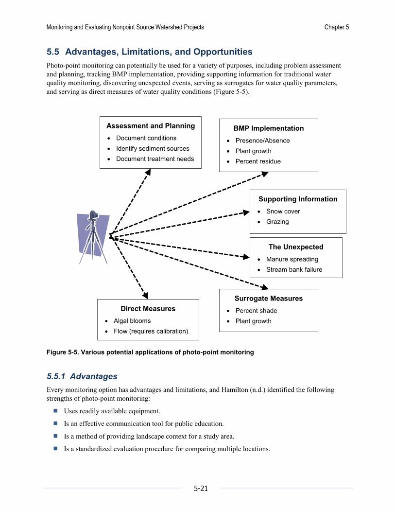
5.5 Advantages, Limitations, and Opportunities Photo-point monitoring can potentially be used for a variety of purposes, including problem assessment and planning, tracking BMP implementation, providing supporting information for traditional water quality monitoring, discovering unexpected events, serving as surrogates for water quality parameters, and serving as direct measures of water quality conditions (Figure 5-5).

BMP Implementation • Presence/Absence• Plant growth• Percent residue

Supporting Information • Snow cover• Grazing

The Unexpected • Manure spreading• Stream bank failure

Surrogate Measures • Percent shade• Plant growth

Direct Measures • Algal blooms• Flow (requires calibration)

Assessment and Planning • Document conditions• Identify sediment sources• Document treatment needs

Figure 5-5. Various potential applications of photo-point monitoring

5.5.1 Advantages Every monitoring option has advantages and limitations, and Hamilton (n.d.) identified the following strengths of photo-point monitoring:

Uses readily available equipment.

Is an effective communication tool for public education.

Is a method of providing landscape context for a study area.

Is a standardized evaluation procedure for comparing multiple locations.


5-22

Is a method to document rates of change.

In addition to these observations, photo-point monitoring is less expensive than most other watershed project monitoring options.

5.5.2 Limitations Some weaknesses of photo-point monitoring were also identified by Hamilton (n.d.):

Only limited quantitative data can be obtained.

Bias in photo point placement may occur.

It may be difficult to use in dense vegetation.

Photo points can be lost or obscured over time.

An additional limitation of photo-point monitoring for watershed projects is that, in most cases, it cannot be used to evaluate progress in achieving water quality objectives. Further, statistical approaches to using photo-derived data remain to be developed for use by those who apply photo-point monitoring techniques.

5.5.3 Opportunities Recognizing the inherent advantages and limitations of photo-point monitoring, there are many opportunities to use this tool for watershed projects. Several of these opportunities have been realized, while others are suggested only for consideration, with full understanding that any method must be tested and evaluated before being adopted.

Photo-point monitoring can be very helpful in assessing watershed problems. For example, it was used in a volunteer-led river continuity assessment of the Ashuelot River water in New Hampshire (Bechtel 2005). Photos were taken at each dam site (at the downstream end) and at both the upstream and downstream ends of stream crossings. The QA officer used the photographs to ensure that information recorded regarding bridge and culvert type made sense. Photos were also used as part of the permanent inventory record.

Photo-point monitoring for western grazing lands has been found to be an easy and inexpensive way to provide an excellent visual representation of conditions at a given point in time. These photographs were considered only as supplementary data, however, not sufficient alone to evaluate objectives (Bauer and Burton 1993). Photographs could be used to indicate a trend in woody vegetation, streambank stability, and streambank cover, but the authors noted that vegetation “expression” as seen in photographs was not the same as vegetation “succession” needed for stream ecosystem health.

At the farm-scale, researchers at the University of Wisconsin-Platteville have applied photo-point monitoring to farm-scale research. Photos have been used for a variety of applications as seen in the sidebar (Busch and Mentz, 2012).

As an example of new applications of photo-point monitoring, it is feasible that photo-point monitoring could be used to track flow provided that a stage-discharge relationship is first established. While this may at first seem to offer no advantage over visual observation of a staff gage, tracking stage with photographs could offer the advantages of 24-hour surveillance and safety during high-flow events.


5-23

Cameras would need to be positioned in secure locations, however, and remote transmission of photos may be required.

The greatest opportunity for photo-point monitoring at the watershed scale, however, may be an improvement in the quantification of variables of interest and statistical analysis of photo-derived data. All monitoring is limited by sample size and representativeness but interpretation of water chemistry monitoring data, for example, is supported by a long history of statistical analysis. Photo-point monitoring for watershed projects has almost no history of statistical analysis. Numeric data are needed for statistical analysis. The primary challenge for those who want to pursue low-cost photo-point monitoring options for project evaluation is to develop more quantitative data and put that data through statistical analyses to create a record of achievement and potential.

Photographic Data Collected at UW-Platteville Pioneer Farm

Researchers at the University of Wisconsin-Platteville have applied photo-point monitoring to farm-scale research. Photographs are used to identify areas of concern, record field conditions within research project areas, monitor the locations of grazing cattle, record unusual or atypical events, and support QA/QC efforts in the surface-water runoff monitoring program. Photographs can be especially useful to convey information to off-site researchers.

Time-lapse photos are taken on a 24-hr interval at surface-water gauging stations to create a record of field conditions within monitored areas. These photographs are useful in determining soil cover, plant canopy, snow cover, and crop growth throughout the year- especially at times when runoff events occur. Moreover, photographs of surface water runoff sample bottles are taken after collectionand prior to lab analysis (Figure 1). While bottle photos provide only qualitative information, such as relative sample color, this information, along with time-lapse photos can help confirm results when laboratory test results are in question. Photos of the bottle tops are used as part of the chain of custody record and project QA/QC, providing an accurate record of samples shipped for analysis.

Figure 1. Sample bottles

Daily time-lapse photos have also been used both to identify paddocks where cattle are grazing in riparian corridors, and to record pasture vegetation height and density. In studies where the location of grazing cattle needs to be recorded daily, landscape photographs can identify the paddocks in which cattle are grazing on a daily basis (Figure 2). Plot photos of pasture vegetation have been used to create a visual record of pasture condition and grass height for runoff studies as well (Figure 3).

Figure 2. Grazing cattle

Figure 3. Pasture vegetation

Photographs are often taken to record extreme events and unusual field observations. For example, photographs have been taken of high-flow events where water depth was greater than the flume height and runoff water flowed over the wing walls holding the flume (Figure 4). Information from these photos can be used to confirm recorded maximum stage readings, and estimate discharge by providing information that can be used to calculate cross-section flow area that occurs above the flume.

Figure 4. Flume


5-24


5-25

5.6 References Bauer, S.B. and T.A. Burton. 1993. Monitoring Protocols to Evaluate Water Quality Effects of Grazing

Management on Western Rangeland Streams. EPA 910/R-93-017. U.S. Environmental Protection Agency, Water Division, Seattle, WA. Accessed February 10, 2016.

Bechtel, D.A. 2005. River Continuity Assessment of the Ashuelot River Watershed Quality Assurance Project Plan. The Nature Conservancy, New Hampshire Chapter, Concord, NH. Accessed February 10, 2016. http://des.nh.gov/organization/divisions/water/wmb/was/qapp/documents/ashuelot.pdf.

Bledsoe, B.P., and J.E. Meyer. 2005. Monitoring of the Little Snake River and Tributaries Year 5 – Final Report. Colorado State University, Department of Civil Engineering, Ft. Collins, CO. Accessed February 10, 2016. http://www.wildlandhydrology.com/assets/Monitoring_of_the_Little_Snake_River_Year_5_Final_Report.pdf.

Busch, D. and R. Mentz. 2012. Photographic Data Collected at UW-Platteville Pioneer Farm. University of Wisconsin-Platteville, Platteville, WI.

CCRWQCB (Central Coast Regional Water Quality Control Board). 2012a. Water Quality Success Stories: Rural Roads Erosion Control Assistance in Santa Cruz County, California. Central Coast Regional Water Quality Control Board, San Luis Obispo, CA. Accessed February 10, 2016. http://www.waterboards.ca.gov/centralcoast/about_us/docs/success/rural_roads.pdf.

CCRWQCB (Central Coast Regional Water Quality Control Board). 2012b. Water Quality Success Stories: The Morro Bay National Monitoring Program - a Ten-Year Rangeland Management Practices Study. Central Coast Regional Water Quality Control Board, San Luis Obispo, CA. Accessed February 10, 2016. http://www.waterboards.ca.gov/centralcoast/about_us/morrobay.shtml.

CCRWQCB (Central Coast Regional Water Quality Control Board) and CPSU (California Polytechnic State University). 2003. Morro Bay National Monitoring Program: Nonpoint Source Pollution and Treatment Measure Evaluation for the Morro Bay Watershed 1992-2002 Final Report. Prepared for U.S. Environmental Protection Agency, by Central Coast Regional Water Quality Control Board and California Polytechnic State University – San Luis Obispo, CA. Accessed February 10, 2016. http://www.elkhornsloughctp.org/uploads/files/1149032089MorroBayEstuaryProgram.pdf.

Clausen, John C., University of Connecticut, Department of Natural Resources and the Environment. 2011. Telephone conversation with Steve Dressing, Tetra Tech, Inc., regarding Jordan Cove Section 319 National Monitoring Program project. Accessed February 10, 2016. See http://jordancove.uconn.edu/index.html for additional details.

Eck, K.J. and D.E. Brown. 2004. Estimating Corn and Soybean Residue Cover. AY-269-W. Purdue University Cooperative Extension Service, West Lafayette, IN. Accessed February 10, 2016. http://www.extension.purdue.edu/extmedia/AY/AY-269-W.pdf.

ERS (Environment and Resource Sciences). 2010. Land Manager’s Monitoring Guide – Photopoint Monitoring. State of Queensland Department of Environment and Resource Management,

http://nepis.epa.gov/Exe/ZyNET.exe/9100QSR9.txt?ZyActionD=ZyDocument&Client=EPA&Index=1991%20Thru%201994&Docs=&Query=910R93017&Time=&EndTime=&SearchMethod=2&TocRestrict=n&Toc=&TocEntry=&QField=&QFieldYear=&QFieldMonth=&QFieldDay=&UseQField=&IntQFieldOp=0&ExtQFieldOp=0&XmlQuery=&File=D%3A%5CZYFILES%5CINDEX%20DATA%5C91THRU94%5CTXT%5C00000025%5C9100QSR9.txt&User=ANONYMOUS&Password=anonymous&SortMethod=h%7C-&MaximumDocuments=15&FuzzyDegree=0&ImageQuality=r85g16/r85g16/x150y150g16/i500&Display=hpfr&DefSeekPage=x&SearchBack=ZyActionL&Back=ZyActionS&BackDesc=Results%20page&MaximumPages=1&ZyEntry=1&SeekPage=x

http://nepis.epa.gov/Exe/ZyNET.exe/9100QSR9.txt?ZyActionD=ZyDocument&Client=EPA&Index=1991%20Thru%201994&Docs=&Query=910R93017&Time=&EndTime=&SearchMethod=2&TocRestrict=n&Toc=&TocEntry=&QField=&QFieldYear=&QFieldMonth=&QFieldDay=&UseQField=&IntQFieldOp=0&ExtQFieldOp=0&XmlQuery=&File=D%3A%5CZYFILES%5CINDEX%20DATA%5C91THRU94%5CTXT%5C00000025%5C9100QSR9.txt&User=ANONYMOUS&Password=anonymous&SortMethod=h%7C-&MaximumDocuments=15&FuzzyDegree=0&ImageQuality=r85g16/r85g16/x150y150g16/i500&Display=hpfr&DefSeekPage=x&SearchBack=ZyActionL&Back=ZyActionS&BackDesc=Results%20page&MaximumPages=1&ZyEntry=1&SeekPage=x

http://des.nh.gov/organization/divisions/water/wmb/was/qapp/documents/ashuelot.pdf

http://www.wildlandhydrology.com/assets/Monitoring_of_the_Little_Snake_River_Year_5_Final_Report.pdf

http://www.wildlandhydrology.com/assets/Monitoring_of_the_Little_Snake_River_Year_5_Final_Report.pdf

http://www.waterboards.ca.gov/centralcoast/about_us/docs/success/rural_roads.pdf

http://www.waterboards.ca.gov/centralcoast/about_us/morrobay.shtml

http://www.elkhornsloughctp.org/uploads/files/1149032089MorroBayEstuaryProgram.pdf

http://jordancove.uconn.edu/index.html

http://www.extension.purdue.edu/extmedia/AY/AY-269-W.pdf


5-26

Environment and Resource Sciences, Brisbane. Accessed February 10, 2016. http://www.granitenet.com.au/assets/files/Landcare/rabbits_photopoint_indicator_aug2010.pdf.

Eyre, T.J., A.L. Kelly, and V.J. Neldner. 2011. Method for the Establishment and Survey of Reference Sites for Biocondition Version 2.0. State of Queensland Department of Environment and Resource Management, Biodiversity and Ecological Sciences Unit, Brisbane. Accessed February 10, 2016. https://www.qld.gov.au/environment/assets/documents/plants-animals/biodiversity/reference-sites-biocondition.pdf.

Eyre, T.J., A.L. Kelly, V.J. Neldner, B.A. Wilson, D.J. Ferguson, M.J. Laidlaw, and A.J. Franks. 2015. Biocondition: a Condition Assessment Framework for Terrestrial Biodiversity in Queensland. Assessment Manual. Version 2.2. State of Queensland Department of Environment and Resource Management, Biodiversity and Ecosystem Sciences, Brisbane. Accessed February 10, 2016. https://www.qld.gov.au/environment/assets/documents/plants-animals/biodiversity/biocondition-assessment-manual.pdf.

Faux, R.N., P. Maus, H. Lachowski, C.E. Torgersen, and M.S. Boyd. 2001. New Approaches for Monitoring Stream Temperature: Airborne Thermal Infrared Remote Sensing. U.S. Department of Agriculture, Forest Service, Remote Application Center, Integrating & Monitoring Steering Committee, San Dimas, CA. Accessed February 10, 2016. http://www.fs.fed.us/eng/techdev/IM/rsac_reports/TIR.pdf.

GeoSpatial Experts. 2004. Introduction to GPS-Photo Link. U.S. Department of Agriculture, Natural Resources Conservation Service, NE. Accessed February 10, 2016. GPS-Photo_Link_step_by_step.ppt

GeoSpatial Experts. 2016. Geotagging and Photo Mapping Software. Geospatial Experts, Inc., Thornton, CO. Accessed February 10, 2016. http://www.geospatialexperts.com/geotagging.php.

Hall, Frederick C. 2001. Ground-Based Photographic Monitoring. General Technical Report PNW-GTR-503. U.S. Department of Agriculture, Forest Service, Pacific Northwest Research Station, Portland, OR. Accessed February 11, 2016. http://www.fs.fed.us/pnw/publications/pnw_gtr503/.

Hall, Frederick C. 2002. Photo Point Monitoring Handbook. General Technical Report PNW-GTR-526. U.S. Department of Agriculture, Forest Service, Pacific Northwest Research Station, Portland, OR. Accessed February 10, 2016. http://www.fs.fed.us/pnw/pubs/gtr526/.

Hamilton, R.M. n.d. Photo Point Monitoring, aWeed Manager’s Guide to Remote Sensing and GIS — Mapping & Monitoring. U.S. Department of Agriculture, Forest Service, Remote Sensing Applications Center, Salt Lake City, UT. Accessed February 10, 2016. http://www.fs.fed.us/eng/rsac/invasivespecies/documents/Photopoint_monitoring.pdf.

Herrick, J.E., J.W. Van Zee, K.M. Havstad, L.M. Burkett, and W.G. Whitford. 2005. Monitoring Manual for Grassland, Shrubland and Savanna Ecosystems - Volume I: Quick Start. U.S. Department of Agriculture, Agricultural Research Service Jornada Experimental Range, Las Cruces, NM. Accessed February 10, 2016. http://www.ntc.blm.gov/krc/viewresource.php?courseID=281&programAreaId=148.

Herrick, J.E., J.W. Van Zee, K.M. Havstad, L.M. Burkett, and W.G. Whitford. 2005a. Monitoring Manual for Grassland, Shrubland and Savanna Ecosystems - Volume II: Design, Supplementary

http://www.granitenet.com.au/assets/files/Landcare/rabbits_photopoint_indicator_aug2010.pdf

https://www.qld.gov.au/environment/assets/documents/plants-animals/biodiversity/reference-sites-biocondition.pdf

https://www.qld.gov.au/environment/assets/documents/plants-animals/biodiversity/reference-sites-biocondition.pdf

https://www.qld.gov.au/environment/assets/documents/plants-animals/biodiversity/biocondition-assessment-manual.pdf

https://www.qld.gov.au/environment/assets/documents/plants-animals/biodiversity/biocondition-assessment-manual.pdf

http://www.fs.fed.us/eng/techdev/IM/rsac_reports/TIR.pdf

https://efotg.sc.egov.usda.gov/references/public/NE/GPS-Photo_Link_step_by_step.ppt

https://efotg.sc.egov.usda.gov/references/public/NE/GPS-Photo_Link_step_by_step.ppt

http://www.geospatialexperts.com/geotagging.php

http://www.fs.fed.us/pnw/publications/pnw_gtr503/

http://www.fs.fed.us/pnw/pubs/gtr526/

http://www.fs.fed.us/eng/rsac/invasivespecies/documents/Photopoint_monitoring.pdf

http://www.ntc.blm.gov/krc/viewresource.php?courseID=281&programAreaId=148


5-27

Methods And Interpretation, U.S. Department of Agriculture, Agricultural Research Service Jornada Experimental Range, Las Cruces, NM. Accessed February 10, 2016. http://www.ntc.blm.gov/krc/viewresource.php?courseID=281&programAreaId=148.

Hickman, J.S. and D.L. Schoenberger. 1989. Wheat Residue. Bulletin L-781. Kansas State University, Cooperative Extension Service, Manhattan, KS. Accessed February 10, 2016. http://www.ksre.ksu.edu/bookstore/pubs/L781.pdf.

Hively, W.D., M. Lang, G.W. McCarty, J. Keppler, A. Sadeghi, and L.L. McConnell. 2009a. Using satellite remote sensing to estimate winter cover crop nutrient uptake efficiency. Journal of Soil and Water Conservation 64(5):303-313.

Hively, W.D., G.W. McCarty, and J. Keppler. 2009b. Federal-state partnership yields success in remote sensing analysis of conservation practice effectiveness: results from the Choptank River Conservation Effects Assessment Project. Journal of Soil and Water Conservation 64(5):154A.

Key, C. H., D. B. Fagre, and R. K. Menicke. 2002. Glacier Retreat in Glacier National Park, Montana. In Satellite Image Atlas of Glaciers of the World, Glaciers of North America - Glaciers of the Western United States. U.S. Geological Survey Professional Paper 1386-J, R.M. Krimmel, pp. J365-J381. Accessed February 10, 2016. http://nrmsc.usgs.gov/files/norock/products/GCC/SatelliteAtlas_Key_02.pdf.

Kinney, J.W. and W.P. Clary. 1994. A Photographic Utilization Guide for Key Riparian Graminoids. General Technical Report INT-GTR-308. U.S. Department of Agriculture, Forest Service, Intermountain Research Station, Ogden, UT. Accessed February 10, 2016. http://www.fs.fed.us/rm/pubs_int/int_gtr308.html.

Kinney, J.W. and W.P. Clary. 1998. Time-Lapse Photography to Monitor Riparian Meadow Use. USDA Forest Service Research Note RMRS-RN-5. U.S. Department of Agriculture, Forest Service, Rocky Mountain Research Station, Boise, ID. Accessed February 10, 2016. http://www.fs.fed.us/rm/pubs/rmrs_rn005.pdf.

Larsen, D. 2006. Minimum Standards for Nebraska NRCS Photo-Point Monitoring. Range and Pasture Technical Note No.16. U.S. Department of Agriculture, Natural Resources Conservation Service. Accessed February 10, 2016. http://efotg.sc.egov.usda.gov/references/public/NE/NE_TECH_NOTE_16.pdf.

MathWorks. 2012. MATLAB Image Processing Toolbox. MathWorks, Natick, MA. Accessed February 10, 2016. http://www.mathworks.com/products/image/.

MMC (Mosman Municipal Council). n.d. Chinamans Beach Photo Point Monitoring Program Spring/Summer 2004 & Autumn/Winter 2005. Mosman Municipal Council, Mosman, Australia.

MST (Missouri Stream Team). n.d. Stream Team Photo Point Monitoring. Missouri Stream Team, Jefferson City, MO. Accessed February 10, 2016. http://www.mostreamteam.org/Documents/STActivities/ppmonitoring.pdf.

NMED (New Mexico Environment Department). 2009. Watershed Protection Section Clean Water Act §319(H) Projects 1998 – 2008. New Mexico Environment Department, Surface Water Quality Bureau.

http://www.ntc.blm.gov/krc/viewresource.php?courseID=281&programAreaId=148

http://www.ksre.ksu.edu/bookstore/pubs/L781.pdf

http://nrmsc.usgs.gov/files/norock/products/GCC/SatelliteAtlas_Key_02.pdf

http://www.fs.fed.us/rm/pubs_int/int_gtr308.html

http://www.fs.fed.us/rm/pubs/rmrs_rn005.pdf

http://efotg.sc.egov.usda.gov/references/public/NE/NE_TECH_NOTE_16.pdf

http://www.mathworks.com/products/image/

http://www.mostreamteam.org/Documents/STActivities/ppmonitoring.pdf


5-28

OEPA (Ohio Environmental Protection Agency). n.d. Ohio Section 319 Success Story: Wetland Restoration in the Sandusky Watershed. Ohio Environmental Protection Agency, Columbus, OH. Accessed February 11, 2016. http://www.epa.ohio.gov/portals/35/nps/319DOCS/Wetlands%20Restoration%20in%20Northern%20Sandusky%20Watershed.pdf.

Oregon DEQ (Department of Environmental Quality). 2002. Oregon 2002 Nonpoint Source Pollution Program Annual Report. Oregon Department of Environmental Quality, Water Quality Division, Portland, OR. Accessed February 11, 2016. http://www.deq.state.or.us/wq/nonpoint/docs/annualrpts/rpt02.pdf.

PCEI (Palouse-Clearwater Environmental Institute). 2005. South Fork Palouse River - Lower Watershed Restoration Project Final Report. Palouse-Clearwater Environmental Institute, Moscow, ID.

Rasmussen J., M. Nørremark, and B.M. Bibby. 2007. Assessment of leaf cover and crop soil cover in weed harrowing research using digital images. Weed Research 47, 299–310.

Richardson, M.D., D.E. Karcher, and L.C. Purcell. 2001. Quantifying turfgrass cover using digital image analysis. Crop Science 41:1884-1888.

Rosgen, David L., 1973. The Use of Color Infrared Photography for the Determination of Sediment Production. In Fluvial Process and Sedimentation: Proceedings of Hydrology Symposium, Canadian National Research Council, Edmonton, Alberta, May 8-9, 1973, pp. 381-402.

Rosgen, David L., 1976. The Use of Color Infrared Photography for the Determination of Suspended Sediment Concentrations and Source Areas. In Proceedings of the 3rd Inter-Agency Sediment Conference, Water Resources Council, Denver, Colorado, March 22-25, 1976, Chapter 7, pp. 30-42. Accessed February 11, 2016. http://www.wildlandhydrology.com/assets/The_Use_of_Color_Infrared_Photography-FISC.pdf.

Shaff, C., J. Reiher, and J. Campbell. 2007. OWEB Guide to Photo Point Monitoring. Oregon Watershed Enhancement Board, Salem, OR. Accessed February 11, 2016. http://www.oregon.gov/OWEB/docs/pubs/PhotoPoint_Monitoring_Doc_July2007.pdf?ga=t.

Shelton, D.P., P.J. Jasa, J.A. Smith, and R. Kanable. 1995. G95-1132 Estimating Percent Residue Cover. Paper 784. Historical Materials from University of Nebraska-Lincoln Extension. Accessed February 11, 2016. http://digitalcommons.unl.edu/extensionhist/784/.

SOLVE. 2011. Adventures in Monitoring. SOLVE Green Team, Oregon. Accessed February 11, 2016. http://solvgreenteam.wordpress.com/tag/photo-point-monitoring/.

USDA-CES (U.S. Department of Agriculture, Cooperative Extension Service), USDA-NRCS (U.S. Department of Agriculture, Natural Resources Conservation Service), and USDOI-BLM (U.S. Department of Interior-Bureau of Land Management). 1999. Utilization Studies and Residual Measurements. Interagency Technical Reference 1734-3. U.S. Department of Agriculture, Cooperative Extensive Service and Natural Resources Conservation Service and U.S. Department of the Interior, Bureau of Land Management, Denver, CO. Accessed February 11, 2016. http://www.blm.gov/nstc/library/pdf/utilstudies.pdf.

http://www.epa.ohio.gov/portals/35/nps/319DOCS/Wetlands%20Restoration%20in%20Northern%20Sandusky%20Watershed.pdf

http://www.epa.ohio.gov/portals/35/nps/319DOCS/Wetlands%20Restoration%20in%20Northern%20Sandusky%20Watershed.pdf

http://www.deq.state.or.us/wq/nonpoint/docs/annualrpts/rpt02.pdf

http://www.wildlandhydrology.com/assets/The_Use_of_Color_Infrared_Photography-FISC.pdf

http://www.oregon.gov/OWEB/docs/pubs/PhotoPoint_Monitoring_Doc_July2007.pdf?ga=t

http://digitalcommons.unl.edu/extensionhist/784/

http://solvgreenteam.wordpress.com/tag/photo-point-monitoring/

http://www.blm.gov/nstc/library/pdf/utilstudies.pdf


5-29

USDA-FS (U.S. Department of Agriculture, Forest Service). 2007. Removal of Marmot Dam. U.S. Department of Agriculture, Forest Service, Mt. Hood National Forest, Sandy, OR. Accessed February 11, 2016. http://www.fs.usda.gov/detail/mthood/home/?cid=STELPRDB5200643 and http://or.water.usgs.gov/projs_dir/marmot/index.html.

USEPA (U.S. Environmental Protection Agency). 2008. Handbook for Developing Watershed Plans to Restore and Protect Our Waters. EPA 841-B-08-002. U.S. Environmental Protection Agency, Office of Water, Washington, DC. Accessed February 10, 2016. http://www.epa.gov/polluted-runoff-nonpoint-source-pollution/handbook-developing-watershed-plans-restore-and-protect.

USSARTF (United States Search and Rescue Task Force). n.d. Compass Basics, United States Search and Rescue Task Force, Elkins Park, PA. Accessed February 11, 2016. http://www.ussartf.org/compass_basics.htm.

Wolfram. 2012. Mathematica. Wolfram Research, Champaign, IL. Accessed February 11, 2016. http://www.wolfram.com/mathematica/?source=nav.

http://www.fs.usda.gov/detail/mthood/home/?cid=STELPRDB5200643

http://or.water.usgs.gov/projs_dir/marmot/index.html

http://www.epa.gov/polluted-runoff-nonpoint-source-pollution/handbook-developing-watershed-plans-restore-and-protect

http://www.epa.gov/polluted-runoff-nonpoint-source-pollution/handbook-developing-watershed-plans-restore-and-protect

http://www.ussartf.org/compass_basics.htm

http://www.wolfram.com/mathematica/?source=nav


5-30

This page intentionally left blank.