Embed Size (px)
Citation preview

Section 5.0 Estimating Exposure Point Concentrations
5-1
5.0 Estimating Exposure Point ConcentrationsExposure point concentrations are constituent concentrations at the location in the
environment where a receptor may be exposed. To determine constituent concentrations inenvironmental media with which a receptor comes in contact (e.g., groundwater, air, soil),several computer-based models and sets of equations are used. Generally, these include
� Source partition models � Fate and transport models � Farm food chain equations� Aquatic food chain equations.
The three types of waste management units evaluated in this risk assessment aredescribed in detail in Section 4.0. For this risk assessment, it was assumed that paint wastes aredeposited in industrial landfills, treatment tanks, and surface impoundments. Chemicalconstituents found in paint waste are released from these WMUs into the surroundingenvironment. Releases to the atmosphere occur through volatilization of vapors from all threeWMU types. Particulates are released from landfills by wind erosion from the surface of thelandfill. Leachate is formed and migrates to groundwater from both landfills and surfaceimpoundments. These materials are then transported by various mechanisms to the air, soil,surface water, and groundwater in the environment immediately surrounding the WMU. Once inthe environment, constituents may move into the human food chain by contaminating fruits,vegetables, beef, milk, and fish consumed by humans. Constituents in the environment may alsomove into the ecological food web by contaminating plants and prey consumed by wildlife.
This risk analysis was performed in both a deterministic and probabilistic or Monte Carlomode. Section 3.0 explains in detail the risk assessment framework, including the structure ofthe deterministic and Monte Carlo analyses. The models and algorithms described in this sectionwere used for both types of analyses. Although the calculations were identical for these twotypes of analyses, the model input parameter values differed. In the deterministic analyses, themodel input parameter values were fixed and a single set of results was generated. In the MonteCarlo analysis, certain model input parameter values were varied in each of 10,000 iterations togenerate a distribution of media concentrations.
The following subsections describe these models and equations and their application inthis risk assessment. Section 5.1 describes the source partition models used to predictenvironmental releases of constituents from WMUs. Section 5.2 discusses the air dispersion anddeposition modeling and methodologies used to estimate constituent-specific soil and waterconcentrations used in the human health and ecological risk analyses. Groundwater modeling isalso presented in Section 5.2, as are the calculations of indoor air concentrations associated with
Section 5.0 Estimating Exposure Point Concentrations
5-2
domestic use of contaminated groundwater. The methodology for calculating food chainconcentrations based on air, soil, and water concentrations is discussed in Section 5.3.
Greater detail is provided in appendixes to this document:
� Appendix F, Variable Summary of Aboveground Fate and Transport Model. Theinput values or distributions used in the algorithms presented in Appendix M arepresented and referenced in this appendix.
� Appendix K, Modifications to HWIR Source Partition Model Programs. Thisappendix explains the changes made to the source partition models for use in thisrisk assessment.
� Appendix L, Source Data. The source partition model input parameter valuesused in this risk assessment are presented in this appendix for landfills, treatmenttanks, and surface impoundments.
� Appendix M, Indirect and Direct Exposure Equations. Algorithms used tocalculate air pathway exposure point concentrations for soil, water, terrestrial foodchain, and aquatic food chain are documented in this appendix.
� Appendix N, Air Dispersion and Deposition Modeling. This appendix provideddetails on the air dispersion and deposition modeling for this risk assessment.
� Appendix O, Groundwater Modeling Parameters. The input values ordistributions used in the groundwater modeling are presented in this appendix.
� Appendix P, Shower Model. This appendix documents the algorithms used tocalculate indoor exposure point concentrations due to showering withcontaminated groundwater.
5.1 Source Partition Modeling of Constituent Releases
Source partition models were used to estimate environmental releases of constituentsfrom landfills, treatment tanks, and surface impoundments. Each WMU has different releasemechanisms that determine the environmental media impacted:
� Landfills. Wastes managed in off-site industrial landfills can release COCs asvapors or particles to the air via windblown erosion or as leachate to thegroundwater.
� Tanks. Wastes managed in tanks can release COCs into the atmosphere viavolatilization. Because tanks contain liquid waste, particulate emissions are notreleased or do not occur from this WMU. Waste in the tanks was assumed not toleak so that no direct releases to the groundwater or soil occur.
Section 5.0 Estimating Exposure Point Concentrations
5-3
� Surface Impoundments. Release mechanisms from surface impoundmentsinclude volatilizing to the air and leaching to the groundwater. Because surfaceimpoundments contain liquid waste, particulate emissions are not released or donot occur from this WMU.
Models developed for the Hazardous Waste Identification Rule (HWIR99) for landfills,tanks, and surface impoundments were used to estimate emissions to air and leachate togroundwater from these units. These models were selected because they are considered to bestate-of-the-art models for modeling hazardous waste disposal. Additionally, these models aredynamic, they are based on a mass balance, and they include a rigorous hydrology model. TheHWIR models consider a variety of removal pathways including aerobic and anaerobicbiodegradation, hydrolysis, volatilization, and leaching.
The HWIR models were originally developed to operate within a larger modeling system,which is described in Overview of the FRAMES - HWIR Technology Software System (PNNL,1999). A few basic changes were necessary to allow the model to run as a stand-alone model. These changes are documented in Appendix K.
The source partition models use information for a specific WMU (e.g., surface area),constituent, environmental setting (e.g., precipitation, temperature), and waste stream to estimateenvironmental release of COCs for each release mechanism. Because the purpose of thisassessment was to calculate waste concentrations that are protective of human health and theenvironment, specific waste concentrations were not initially used in the source models. Instead,the models were executed using a unit waste concentration (e.g., 1 mg/kg). Additionally, themodels were initially executed assuming the fraction of waste contaminated (f-wmu) is equal to1. The results of these source model runs were then used to calculate target waste concentrationsin the WMUs. Using waste volume data from the 3007 survey, these target waste concentrationsin the WMUs were scaled to target waste concentrations in the paint waste streams (seeSection 4.2) using procedures described in Section 8.0.
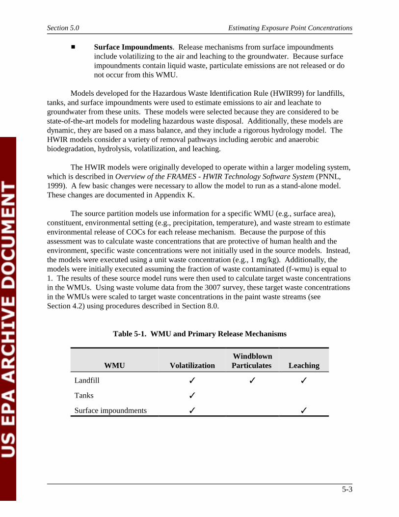
Table 5-1. WMU and Primary Release Mechanisms
WMU VolatilizationWindblownParticulates Leaching
Landfill � � �
Tanks �
Surface impoundments � �
Section 5.0 Estimating Exposure Point Concentrations
5-4
5.1.1 Landfill Partition Model
The landfill model was developed to approximate the dynamic effects of the gradualfilling of active landfills. The landfill is divided into equal-volume vertical cells running fromthe site surface to the bottom of the landfill, each sized so that it requires 1 year to fill. Wastemass is added gradually, forming layers of waste. After 1 year, the cell is full and the waste iscovered with a clean soil cover. Then the next cell begins to fill, and so on until the landfillreaches maximum capacity. Results for the landfill as a whole are then obtained by aggregatingstored results for each single cell to account for the time that each cell in the landfill was filled. For example, the results for the landfill at the end of year 3 are a summation of results for thefirst cell filled at year 3 in the single-cell simulation, the second cell filled at year 2, and the thirdcell filled at year 1.
The active life of a landfill is assumed to be 30 years; therefore, 30 cells were modeled bythe landfill model. The model estimates environmental releases from the landfill beginning inthe first year of operation. The landfill fills for 30 years, after which time no more constituentmass is being added and the model accounts for continuous loss of constituent mass. Thismodeling process continues until 1 percent of the peak constituent mass remains or until 200years, whichever comes first. The peak 9-year average was calculated from the series of annualmodel outputs. These 9-year average results were the inputs to the fate and transport models.Two hundred years was selected as a maximum modeling period because, for most constituents,the peak 9-year average is unchanged by modeling greater than 200 years and, in general, wouldoccur during the last 9 years of its active life. Examination of the source partition modelingresults in this analysis confirmed that this was true for all constituents evaluated.
Other assumptions made in modeling landfills include
� The landfill is assumed to be below grade so that all precipitation that falls ontothe landfill either is evapotranspirated, percolates as infiltration, or increases themoisture content in the unit. That is, storm water run-on, runoff, and erosion areassumed not to occur.
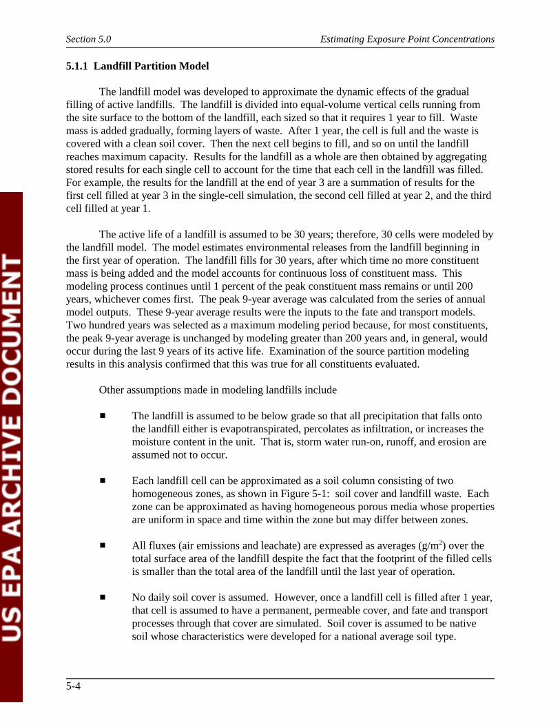
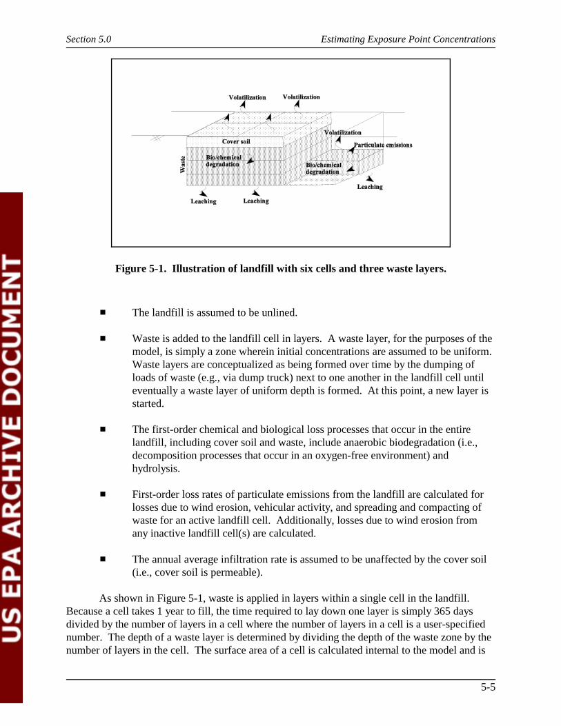
� Each landfill cell can be approximated as a soil column consisting of twohomogeneous zones, as shown in Figure 5-1: soil cover and landfill waste. Eachzone can be approximated as having homogeneous porous media whose propertiesare uniform in space and time within the zone but may differ between zones.
� All fluxes (air emissions and leachate) are expressed as averages (g/m2) over thetotal surface area of the landfill despite the fact that the footprint of the filled cellsis smaller than the total area of the landfill until the last year of operation.
� No daily soil cover is assumed. However, once a landfill cell is filled after 1 year,that cell is assumed to have a permanent, permeable cover, and fate and transportprocesses through that cover are simulated. Soil cover is assumed to be nativesoil whose characteristics were developed for a national average soil type.
Section 5.0 Estimating Exposure Point Concentrations
5-5
Figure 5-1. Illustration of landfill with six cells and three waste layers.
� The landfill is assumed to be unlined.
� Waste is added to the landfill cell in layers. A waste layer, for the purposes of themodel, is simply a zone wherein initial concentrations are assumed to be uniform. Waste layers are conceptualized as being formed over time by the dumping ofloads of waste (e.g., via dump truck) next to one another in the landfill cell untileventually a waste layer of uniform depth is formed. At this point, a new layer isstarted.
� The first-order chemical and biological loss processes that occur in the entirelandfill, including cover soil and waste, include anaerobic biodegradation (i.e.,decomposition processes that occur in an oxygen-free environment) andhydrolysis.
� First-order loss rates of particulate emissions from the landfill are calculated forlosses due to wind erosion, vehicular activity, and spreading and compacting ofwaste for an active landfill cell. Additionally, losses due to wind erosion fromany inactive landfill cell(s) are calculated.
� The annual average infiltration rate is assumed to be unaffected by the cover soil(i.e., cover soil is permeable).
As shown in Figure 5-1, waste is applied in layers within a single cell in the landfill. Because a cell takes 1 year to fill, the time required to lay down one layer is simply 365 daysdivided by the number of layers in a cell where the number of layers in a cell is a user-specifiednumber. The depth of a waste layer is determined by dividing the depth of the waste zone by thenumber of layers in the cell. The surface area of a cell is calculated internal to the model and is
Section 5.0 Estimating Exposure Point Concentrations
5-6
equal to the load (Mg/yr) divided by the depth of the waste layer (m) times the bulk density of thewaste (g/m3) and a units conversion factor. The number of years the landfill operates then is thetotal surface area of the landfill divided by the surface area of a single waste cell.
The landfill model consists of several interacting submodels or algorithms, the mostsignificant of which are
� Generic Soil Column Model (GSCM)
� Hydrology model
� Set of calculations that estimates airborne emissions of particulates (and sorbedconstituent) due to wind erosion or other surface disturbances (e.g., vehiculartraffic).
These three primary submodels are discussed in the following subsections.
5.1.1.1 Generic Soil Column Model. The General Soil Column Model is thefundamental “building block” of the landfill partition model; it describes the dynamic, verticalfate and transport of constituent within a single landfill cell. As stated previously, the GSCMsimulation of the processes in the landfill cell begins in the first year of operation and continuesthrough the filling of the cell (1 year), and thereafter until less than 1 percent of the cell’s peakconstituent mass remains or 200 years—whichever occurs first. The complete time series of theGSCM emissions simulations for the first cell (perhaps 200 years) are stored by the landfillmodel and are then used to represent new cells being filled in subsequent years. The assumptionsand limitations of the GSCM are summarized here and are described in full in the backgrounddocument Source Modules for Nonwastewater Waste Management Units (Land ApplicationUnits, Waste Piles, and Landfills). Background Document and Implementation for theMultimedia, Multipathway, and Multireceptor Risk Assessment (3MRA) for HWIR 99 (U.S. EPA,1999b).
� The medium modeled, whether soil, waste, or a soil/waste mixture, can beapproximated for modeling purposes as an unconsolidated, homogeneous, porousmedium.
� Internal loss processes, which include anaerobic biodegredation and hydrolysiscan be considered to proceed in accordance with first-order reaction kinetics.
� The contaminant partitions to three phases: adsorbed (solid), dissolved (liquid),and gaseous. This partitioning of constituent mass is similar to the methodsdescribed in Jury et al. (1983, 1990).
� Contaminant partitioning between sorbed and aqueous phases is reversible andlinear. Furthermore, the partitioning coefficient is unaffected by changes inconcentrations or environmental conditions (e.g., pH, temperature) during themodel execution.
Section 5.0 Estimating Exposure Point Concentrations
5-7
� Contaminant partitioning between aqueous and gaseous phases can be describedby Henry’s law. The gaseous phase constituent volatilizes from the surface of thelandfill to the air.
� Constituent sorbed to surface materials can be lost to the atmosphere via winderosion or other surface disturbance of particles. These losses are modeled asdescribed in Section 5.1.1.3 and are linked to the GSCM as first-order lossmechanisms.
� The chemical is transported in one dimension through the soil column, a methodsimilar to those methods described in Jury et al. (1983, 1990) and Shan andStephens (1995).
� Formation of chemical species by chemical or biological processes in the landfill(e.g., daughter products) is not considered. (See Appendix T for results of theanalysis conducted to determine whether to consider daughter products.)
� Leaching of aqueous-phase constituent mass occurs by advection or diffusionfrom the bottom of the WMU or vadose zone.
Greater detail on the GSCM algorithms is provided in the HWIR documentation (U.S. EPA,1999b).
5.1.1.2 Hydrology Model. The hydrology model provides estimates of daily soilmoisture, runoff, evapotranspiration, and infiltration. Runoff is assumed to be zero for thebelow-grade landfill. These daily estimates are then used by the GSCM algorithm in its dailytime step to build up the annual average output variable values. Details for the hydrologyalgorithms incorporated into the landfill partition model are described in the HWIRdocumentation (U.S. EPA, 1999b).
5.1.1.3 Particulate Emissions. Particulate chemical fluxes to the atmosphere,representing chemicals sorbed to surficial soils that become airborne, are estimated usingempirical relationships developed by EPA (1995) and Cowherd et al. (1985). Using theserelationships, the landfill model estimates the total emission rate of contaminants sorbed ontoparticles that are 30 �m or smaller. In addition, the landfill model estimates the particle sizedistribution of these emitted solids.
The empirical relationships were developed for specific surface-disturbing activities,consisting of wind erosion, vehicular activity (trucks driving on the landfill surface), wasteunloading activities, and waste spreading/compacting activities. For each of these activities, anactivity-specific particle size distribution was estimated by EPA (1995), consisting of fourparticle size categories: 30 to 15 �m, 15 to 10 �m, 10 to 2.5 �m, and less than 2.5 �m. Thelandfill model estimates the total mass flux of 30 �m or smaller particles being emitted by thesevarious surface disturbances and, based on the fraction of this total from each disturbanceactivity, calculates the resulting particle size distribution by mass-weighting the componentdistributions. It should be noted, however, that, when the ISC air model is run prior to the
Section 5.0 Estimating Exposure Point Concentrations
5-8
landfill model (as was necessary for this project due to scheduling constraints), this landfillmodel-generated, run-specific particle size distribution is not available for ISC. In addition, inorder to use the landfill-model-generated particle size distributions, the ISC model would havehad to be run for each iteration of the Monte Carlo simulation. Given these time constraints, adefault distribution based on wind erosion only was assumed for the ISC model. The defaultwind-erosion-only distribution is: 30 to 15 �m (40 percent), 15 to 10 �m (10 percent), 10 to 2.5�m (30 percent), and less than 2.5 �m (20 percent). While some paint waste such as emissioncontrol dust may be made up primarily of the smaller size particles, we assumed for this analysisthat the waste material becomes well-mixed with other wastes and soils before being emitted as aparticulate; therefore the default distribution (based on wind-eroded soil particles) is assumed toremain applicable.
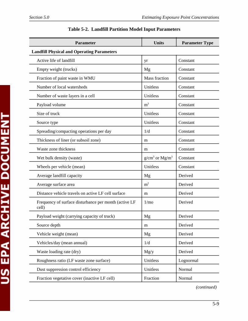
5.1.1.4 Model Input Parameters for Landfill Model. The input parameters for thelandfill model can be categorized into physical, operating, meteorological, soil, vadose, bulkwaste, waste stream, and chemical input parameters. These parameters were developed for 68landfills, 49 meteorological sites, 2 waste streams, and 43 constituents. Section 4.3 presents adetailed discussion of the location-dependent parameters, which are based on the location of the49 meteorological sites used in this analysis. Table 5-2 presents the WMU model inputs requiredby the landfill model. Details pertaining to the parameter values used in the landfill partitionmodel are presented in Appendix L.
The bulk waste parameters are defined in terms of industrial landfill waste and are notspecific to paint waste. Additionally, it is assumed that soil values are a good representation ofindustrial landfill waste. These parameters were obtained from soils data and used the averagevalue from four soil textures as surrogates. Because these parameters are correlated, empiricaldistributions were developed (see Section 4.3). There were two waste streams modeled withinthe landfill model: emission control dust and combined solids. Because combined solids had asignificantly higher moisture content than dust, these two waste streams were modeledseparately. Constituent-specific parameters are also listed. These parameter values are presentedin Appendixes D and H.
5.1.1.5 Landfill Partition and Model Results. The emission rates (g/s) for particulateand volatile emissions to the air were calculated by the landfill partition model and then used inthe multipathway fate and transport model (where emissions were converted from g/m2-d usingthe surface area of the landfills). Results were generated for 10,000 runs for each of the 43chemicals and for both the combined solids and emission control dust waste streams. Each runwas identified by landfill WMU, meteorological site, and a run ID that corresponded to one ofthe 10,000 Monte Carlo iterations. Central tendency and high-end results were also calculatedfor the deterministic analyses. Section 3.2 discusses the deterministic analysis.
5.1.2 Treatment Tanks
The tank model simulates time-varying releases of constituents to the atmosphere. Thetank unit has only volatile emissions (no particulates) and is assumed to have an imperviousbottom so that there is no contaminant leaching. Therefore, the output from the tank model
Section 5.0 Estimating Exposure Point Concentrations
5-9
Table 5-2. Landfill Partition Model Input Parameters
Parameter Units Parameter Type
Landfill Physical and Operating Parameters
Active life of landfill yr Constant
Empty weight (trucks) Mg Constant
Fraction of paint waste in WMU Mass fraction Constant
Number of local watersheds Unitless Constant
Number of waste layers in a cell Unitless Constant
Payload volume m3 Constant
Size of truck Unitless Constant
Source type Unitless Constant
Spreading/compacting operations per day 1/d Constant
Thickness of liner (or subsoil zone) m Constant
Waste zone thickness m Constant
Wet bulk density (waste) g/cm3 or Mg/m3 Constant
Wheels per vehicle (mean) Unitless Constant
Average landfill capacity Mg Derived
Average surface area m2 Derived
Distance vehicle travels on active LF cell surface m Derived
Frequency of surface disturbance per month (active LFcell)
1/mo Derived
Payload weight (carrying capacity of truck) Mg Derived
Source depth m Derived
Vehicle weight (mean) Mg Derived
Vehicles/day (mean annual) 1/d Derived
Waste loading rate (dry) Mg/y Derived
Roughness ratio (LF waste zone surface) Unitless Lognormal
Dust suppression control efficiency Unitless Normal
Fraction vegetative cover (inactive LF cell) Fraction Normal
(continued)
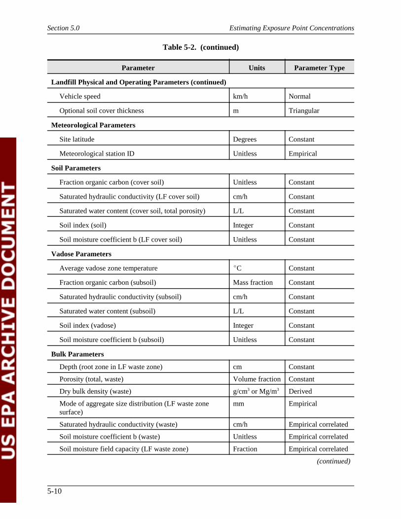
Table 5-2. (continued)
Section 5.0 Estimating Exposure Point Concentrations
Parameter Units Parameter Type
5-10
Landfill Physical and Operating Parameters (continued)
Vehicle speed km/h Normal
Optional soil cover thickness m Triangular
Meteorological Parameters
Site latitude Degrees Constant
Meteorological station ID Unitless Empirical
Soil Parameters
Fraction organic carbon (cover soil) Unitless Constant
Saturated hydraulic conductivity (LF cover soil) cm/h Constant
Saturated water content (cover soil, total porosity) L/L Constant
Soil index (soil) Integer Constant
Soil moisture coefficient b (LF cover soil) Unitless Constant
Vadose Parameters
Average vadose zone temperature �C Constant
Fraction organic carbon (subsoil) Mass fraction Constant
Saturated hydraulic conductivity (subsoil) cm/h Constant
Saturated water content (subsoil) L/L Constant
Soil index (vadose) Integer Constant
Soil moisture coefficient b (subsoil) Unitless Constant
Bulk Parameters
Depth (root zone in LF waste zone) cm Constant
Porosity (total, waste) Volume fraction Constant
Dry bulk density (waste) g/cm3 or Mg/m3 Derived
Mode of aggregate size distribution (LF waste zonesurface)
mm Empirical
Saturated hydraulic conductivity (waste) cm/h Empirical correlated
Soil moisture coefficient b (waste) Unitless Empirical correlated
Soil moisture field capacity (LF waste zone) Fraction Empirical correlated
(continued)
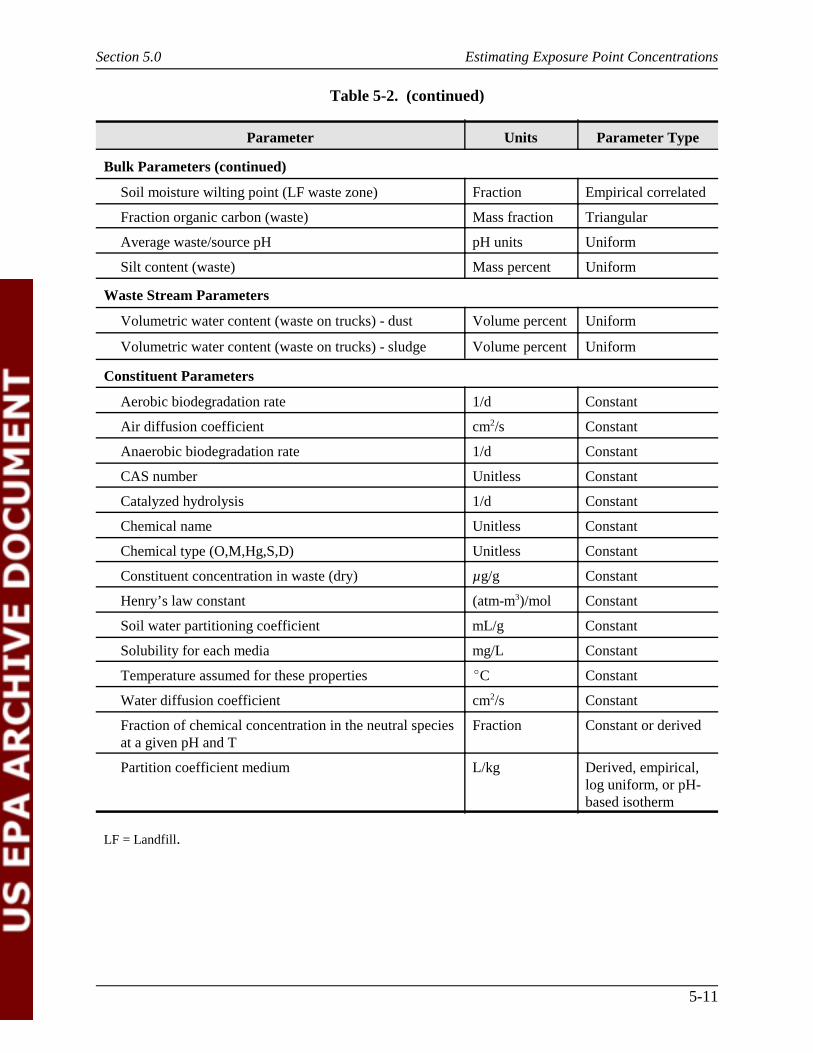
Table 5-2. (continued)
Section 5.0 Estimating Exposure Point Concentrations
Parameter Units Parameter Type
5-11
Bulk Parameters (continued)
Soil moisture wilting point (LF waste zone) Fraction Empirical correlated
Fraction organic carbon (waste) Mass fraction Triangular
Average waste/source pH pH units Uniform
Silt content (waste) Mass percent Uniform
Waste Stream Parameters
Volumetric water content (waste on trucks) - dust Volume percent Uniform
Volumetric water content (waste on trucks) - sludge Volume percent Uniform
Constituent Parameters
Aerobic biodegradation rate 1/d Constant
Air diffusion coefficient cm2/s Constant
Anaerobic biodegradation rate 1/d Constant
CAS number Unitless Constant
Catalyzed hydrolysis 1/d Constant
Chemical name Unitless Constant
Chemical type (O,M,Hg,S,D) Unitless Constant
Constituent concentration in waste (dry) µg/g Constant
Henry’s law constant (atm-m3)/mol Constant
Soil water partitioning coefficient mL/g Constant
Solubility for each media mg/L Constant
Temperature assumed for these properties �C Constant
Water diffusion coefficient cm2/s Constant
Fraction of chemical concentration in the neutral speciesat a given pH and T
Fraction Constant or derived
Partition coefficient medium L/kg Derived, empirical,log uniform, or pH-based isotherm
LF = Landfill.
Section 5.0 Estimating Exposure Point Concentrations
5-12
calculates only release of vapor to the aboveground pathways. The tank model is a quasi-steady-state model, and the emissions occur only while the unit is operating. Volatile emissions werecalculated for 50 years, which is the specified years of operation for treatment tanks in thisanalysis.
The tank model used in this assessment comprises the liquid and sediment components ofthe tank/surface impoundment model developed for HWIR99. A single set of equations andcomputer code has been developed for the liquid and sediment compartments of the modelbecause of similarities in mass balance and transport between tanks and surface impoundments. The primary difference between tanks and surface impoundments is that a tank is assumed tohave an impervious bottom so that there is no contaminant leaching. Both tanks and surfaceimpoundments may be either aerated or quiescent, and the mass transport equations used todescribe volatile contaminant losses from these units are the same. Both units may have somedegree of solids settling. For aerated units, suspended solids in the influent waste primarily passthrough the system with little solids settling (depending on the degree of agitation). Forquiescent units, solids settling and accumulation may be significant. When this occurs, the unithas to be cleaned or dredged to remove the accumulated solids.
This section describes the liquid and sediment compartments that were used to modeltanks. Surface impoundment partition modeling is discussed in Section 5.1.3.
5.1.2.1 Model Overview. The liquid compartment model
� Uses the mass balance approach, taking into consideration contaminant removalby volatilization, biodegradation, hydrolysis, leaching, and partitioning to solids
� Estimates volatilization rates for both aerated and quiescent surfaces
� Estimates suspended solids removal (settling) efficiency
� Estimates temperature effects.
Temporally, a quasi-steady-state monthly time step is used. Quasi-steady-state refers tothe fact that the model employs time steps in its mathematical solution but, within these monthlytime steps, steady-state assumptions are made. Each month, the model updates certainparameters based on average monthly environmental conditions (temperature, windspeed,precipitation, and evaporation). It is then assumed that the system equilibrates instantaneously tothese new conditions and a steady-state solution is obtained for that month. The resulting 12monthly values for all outputs are then averaged and reported as annual averages.
Key Assumptions. The general model construct can be useful for a wide variety ofWMU applications. For this analysis, the following assumptions were used:
� Two-compartment model: "mostly" well-mixed liquid compartment and a well-mixed sediment compartment, which includes a temporary accumulating solidscompartment
Section 5.0 Estimating Exposure Point Concentrations
5-13
� First-order kinetics for volatilization in liquid compartment
� First-order kinetics (e.g., rates of change) for hydrolysis in both liquid andsediment compartment
� First-order kinetics for biodegradation with respect to both contaminantconcentration and biomass concentration in liquid compartment
� First-order kinetics for biodegradation in sediment compartment
� Darcy’s law for calculating the infiltration rate
� First-order kinetics for solids settling
� First-order biomass growth rate with respect to total biological oxygen demand(BOD) loading
� First-order biomass decay rate within the accumulating sediment compartment
� No contaminant in precipitation/rainfall
� Linear contaminant partitioning among adsorbed solids, dissolved phases, andvapor phases
� Daughter products are not included in the model; any constituents generated as areaction intermediate or end product from either biodegradation or hydrolysis arenot included in the model output.
Due to the simplicity of the biodegradation rate model employed and the use of Henry’slaw partitioning coefficients, the model is most applicable to dilute aqueous wastes. At highercontaminant concentrations, biodegradation of toxic constituents may be expected to exhibitzero-order or even inhibitory rate kinetics. For waste streams with high contaminant or high totalorganic concentrations, vapor phase contaminant partitioning may be better estimated usingpartial pressure (Raoult’s law) rather than Henry’s law.
Methodologies. The treatment tank is divided into two primary compartments: a"liquid" compartment and a "sediment" compartment. Mass balances are performed on theseprimary compartments at time intervals small enough that the hydraulic retention time in theliquid compartment is not significantly impacted by the solids settling and accumulation. Figure 5-2 provides a general schematic of a model construct.
In the liquid compartment, there is flow both in and out of the WMU. Solids generationoccurs in the liquid compartment due to biological growth; solids destruction occurs in thesediment compartment due to sludge digestion. Using a well-mixed assumption, the suspendedsolids concentration within the WMU is assumed to be constant throughout the WMU. However, some stratification of sediment is expected across the length and depth of the WMU so

Section 5.0 Estimating Exposure Point Concentrations
5-14
� Rainfall
Influent � � Emissions (aerated and nonaerated surfaces) � Effluent
Liquid Compartment
Aerobic biodegradationFirst-order chemical degradation (e.g., hydrolysis)
Biomass growth
� Contaminant diffusion; � Solids settling/resuspension
Sediment CompartmentAnaerobic degradation/decay
� Solids burial
Figure 5-2. Schematic of general model construct for tanks.
that the effective total suspended solids (TSS) concentration within the tank is assumed to be afunction of the WMU’s TSS removal efficiency rather than equal to the effluent TSSconcentration. The liquid (dissolved) phase contaminant concentration within the tank, however,is assumed to be equal to the effluent dissolved phase concentration (i.e., liquid is well mixed). Consequently, the term "mostly well mixed" is used to describe the liquid compartment.
The steady-state, mass balance assumptions on which the model is based are summarizedas follows.
Constituent Mass Balance in Liquid Compartment. In the liquid compartment, thereis flow both in and out of the WMU. There is also a leachate flow to the sediment compartmentand out the bottom of the WMU for surface impoundments. Within the liquid compartment,there is contaminant loss through volatilization, hydrolysis, and biodegradation. Additionally,contaminant is transported across the liquid/sediment compartment interface by solids settlingand resuspension and by contaminant diffusion.
Constituent Mass Balance in Sediment Compartment. Within the sedimentcompartment, there is contaminant loss through hydrolysis and biodegradation. Additionally,contaminant is transported across the liquid/sediment compartment interface by solids settlingand resuspension and by contaminant diffusion.
Solids Mass Balance in Liquid Compartment. Sedimentation and resuspensionprovide a means of sediment transfer between the liquid and sediment compartments. Sedimentation and resuspension are assumed to occur in the quiescent areas. For systems in
Section 5.0 Estimating Exposure Point Concentrations
5-15
which biodegradation occurs within the liquid compartment, there is also a production ofbiomass associated with the decomposition of organic constituents.
Solids Mass Balance in Sediment Compartment. In the sediment compartment, as inthe liquid compartment, sedimentation and resuspension provide a means of sediment transferbetween the liquid and sediment compartments. In the sediment compartment, however, there issome accumulation of sediment during the time step. This sediment accumulation is alsoreferred to as sediment burial, and the rate of sediment accumulation is determined by the burialvelocity. The primary output of the tank model is the annual average volatilization rate for eachconstituent.
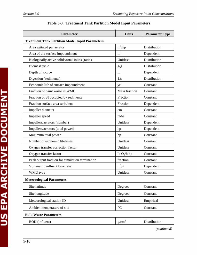
5.1.2.2 Model Input Parameters for Tanks. The input parameters for the tank modelcan be categorized into tank, meteorological, bulk waste, and chemical input parameters. Theseparameters were developed for 200 tanks, 49 meteorological sites, and 43 chemicals. Section 4.3presents a detailed discussion of the location-dependent parameters, which are based on thelocation of the 49 meteorological stations used in this analysis. Table 5-3 presents the WMUmodel inputs required by the tank model. Details pertaining to the parameter values used in thetreatment tank partition model are presented in Appendix L.
Bulk waste parameters are defined in terms of industrial landfill waste and are notspecific to paint waste. Constituent-specific parameters are presented in Appendixes D and H.
5.1.2.3 Treatment Tank Partition Model. The total emission rate (g/s) of volatileemissions to the air was calculated by the treatment tank partition model and then used in themultipathway fate and transport model (where emissions were converted from g/m2-d using thesurface area of the landfills). Results were generated for 10,000 runs for each of the 43chemicals. Each run was identified by tank WMU, meteorological site, and a run ID thatcorresponded to one of the 10,000 Monte Carlo iterations. Central tendency and high-end resultswere also calculated for the deterministic analyses. Section 3.2 discusses the deterministicanalysis.
5.1.3 Surface Impoundments
The surface impoundment model simulates time-varying releases of constituent to theatmosphere. The surface impoundment unit is the same as the tank model, but the bottom of theunit is assumed to be pervious so that contaminant leaching can occur. It is assumed that thereare no direct liquid discharges to the surface due to overflows or structural failures. Therefore,the output from the surface impoundment model provides air emissions as input for calculationsof fate and transport for aboveground pathways and leachate concentration as input forgroundwater pathways. The model is a quasi-steady-state model, and the emissions occur onlywhile the unit operates. The constituent releases are calculated for 50 years, which is thespecified years of operation for surface impoundments in this analysis. After the operatingperiod, the surface impoundment site is assumed to be closed and all constituents removed.
Section 5.0 Estimating Exposure Point Concentrations
5-16
Table 5-3. Treatment Tank Partition Model Input Parameters
Parameter Units Parameter Type
Treatment Tank Partition Model Input Parameters
Area agitated per aerator m2/hp Distribution
Area of the surface impoundment m2 Dependent
Biologically active solids/total solids (ratio) Unitless Distribution
Biomass yield g/g Distribution
Depth of source m Dependent
Digestion (sediments) 1/s Distribution
Economic life of surface impoundment yr Constant
Fraction of paint waste in WMU Mass fraction Constant
Fraction of SI occupied by sediments Fraction Constant
Fraction surface area turbulent Fraction Dependent
Impeller diameter cm Constant
Impeller speed rad/s Constant
Impellers/aerators (number) Unitless Dependent
Impellers/aerators (total power) hp Dependent
Maximum total power hp Constant
Number of economic lifetimes Unitless Constant
Oxygen transfer correction factor Unitless Constant
Oxygen transfer factor lb O2/h-hp Constant
Peak output fraction for simulation termination fraction Constant
Volumetric influent flow rate m3/s Dependent
WMU type Unitless Constant
Meteorological Parameters
Site latitude Degrees Constant
Site longitude Degrees Constant
Meteorological station ID Unitless Empirical
Ambient temperature of site �C Constant
Bulk Waste Parameters
BOD (influent) g/cm3 Distribution
(continued)
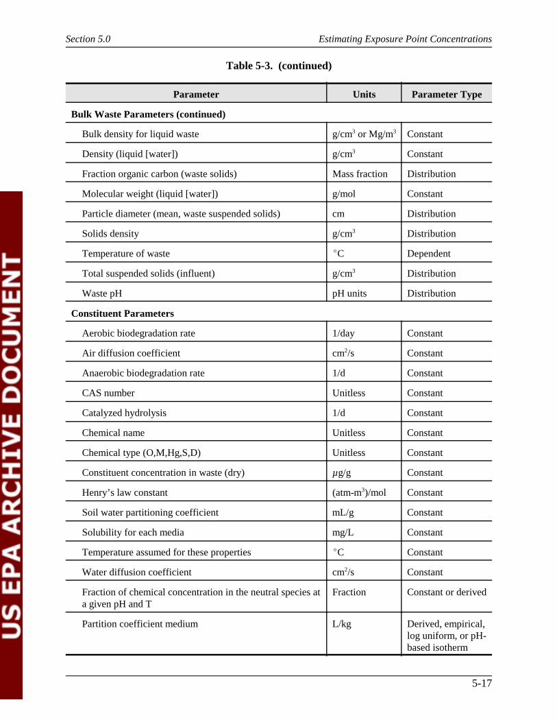
Table 5-3. (continued)
Section 5.0 Estimating Exposure Point Concentrations
Parameter Units Parameter Type
5-17
Bulk Waste Parameters (continued)
Bulk density for liquid waste g/cm3 or Mg/m3 Constant
Density (liquid [water]) g/cm3 Constant
Fraction organic carbon (waste solids) Mass fraction Distribution
Molecular weight (liquid [water]) g/mol Constant
Particle diameter (mean, waste suspended solids) cm Distribution
Solids density g/cm3 Distribution
Temperature of waste �C Dependent
Total suspended solids (influent) g/cm3 Distribution
Waste pH pH units Distribution
Constituent Parameters
Aerobic biodegradation rate 1/day Constant
Air diffusion coefficient cm2/s Constant
Anaerobic biodegradation rate 1/d Constant
CAS number Unitless Constant
Catalyzed hydrolysis 1/d Constant
Chemical name Unitless Constant
Chemical type (O,M,Hg,S,D) Unitless Constant
Constituent concentration in waste (dry) µg/g Constant
Henry’s law constant (atm-m3)/mol Constant
Soil water partitioning coefficient mL/g Constant
Solubility for each media mg/L Constant
Temperature assumed for these properties �C Constant
Water diffusion coefficient cm2/s Constant
Fraction of chemical concentration in the neutral species ata given pH and T
Fraction Constant or derived
Partition coefficient medium L/kg Derived, empirical,log uniform, or pH-based isotherm
Section 5.0 Estimating Exposure Point Concentrations
5-18
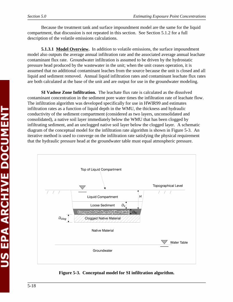
Figure 5-3. Conceptual model for SI infiltration algorithm.
Because the treatment tank and surface impoundment model are the same for the liquidcompartment, that discussion is not repeated in this section. See Section 5.1.2 for a fulldescription of the volatile emissions calculations.
5.1.3.1 Model Overview. In addition to volatile emissions, the surface impoundmentmodel also outputs the average annual infiltration rate and the associated average annual leachatecontaminant flux rate. Groundwater infiltration is assumed to be driven by the hydrostaticpressure head produced by the wastewater in the unit; when the unit ceases operation, it isassumed that no additional contaminant leaches from the source because the unit is closed and allliquid and sediment removed. Annual liquid infiltration rates and contaminant leachate flux ratesare both calculated at the base of the unit and are output for use in the groundwater modeling.
SI Vadose Zone Infiltration. The leachate flux rate is calculated as the dissolvedcontaminant concentration in the sediment pore water times the infiltration rate of leachate flow. The infiltration algorithm was developed specifically for use in HWIR99 and estimatesinfiltration rates as a function of liquid depth in the WMU, the thickness and hydraulicconductivity of the sediment compartment (considered as two layers, unconsolidated andconsolidated), a native soil layer immediately below the WMU that has been clogged byinfiltrating sediment, and an unclogged native soil layer below the clogged layer. A schematicdiagram of the conceptual model for the infiltration rate algorithm is shown in Figure 5-3. Aniterative method is used to converge on the infiltration rate satisfying the physical requirementthat the hydraulic pressure head at the groundwater table must equal atmospheric pressure.
Section 5.0 Estimating Exposure Point Concentrations
5-19
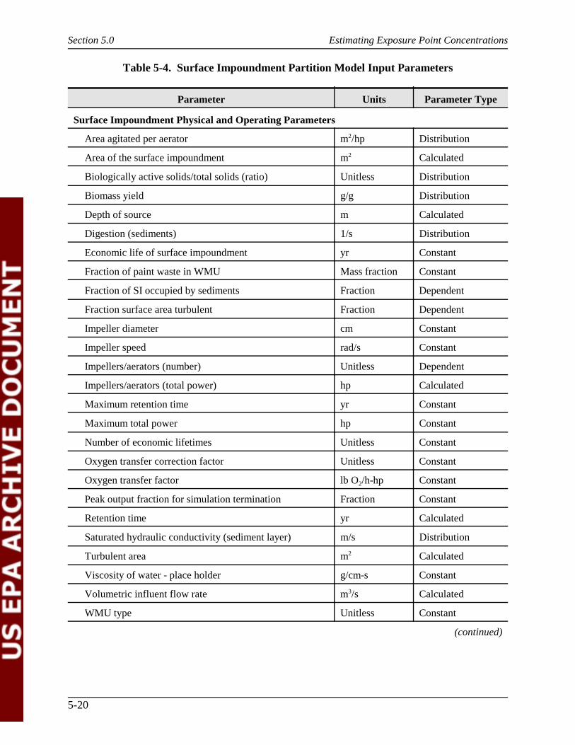
5.1.3.2 Model Input Parameters for Surface Impoundment Source Model. The inputparameters for the surface impoundment model can be categorized into physical and operating,meteorological, vadose, bulk waste, and chemical input parameters. These parameters weredeveloped for 200 surface impoundments, 49 meteorological sites, and 43 chemicals. Section 4.3 presents a detailed discussion of the location-dependent parameters, which are basedon the locations of the 49 meteorological sites used in this analysis. Table 5-4 presents theWMU model inputs required by the surface impoundment model. Details pertaining to theparameter values used in the surface impoundment partition model are presented in Appendix L.
The bulk waste parameters are defined in terms of industrial landfill waste and are notspecific to paint waste. Constituent parameters are presented in Appendixes D and H.
5.1.3.3 Surface Impoundment Partition Model Results. The total emission rate (g/s)of particulate and volatile emissions to the air was calculated by the surface impoundmentpartition model and then used in the multipathway fate and transport model (where emissionswere converted from g/m2-d using the surface area of the surface impoundment). Results weregenerated for 10,000 runs for each of the 43 chemicals. Each run was identified by surfaceimpoundment WMU, meteorological site, and a run ID that corresponded to one of the 10,000Monte Carlo iterations. Central tendency and high-end results were also calculated for thedeterministic analyses. Section 3.2 discusses the deterministic analysis.
5.2 Fate and Transport Modeling
This section describes the methodology and the models that were used to predict the fateand transport of chemical constituents in the environment. The methodology is based on threesources:
� Methodology for Assessing Health Risks Associated with Multiple Pathways ofExposure to Combustor Emissions, Update (U.S. EPA, 1998b)
� Methodology for Assessing Health Risks Associated with Indirect Exposure toCombustor Emissions (U.S. EPA, 1990)
� Human Health Risk Assessment Protocol for Hazardous Waste CombustionFacilities. Volume One (U.S. EPA, 1998a)
Once a constituent is released from a waste management unit, it can move through the air,soil, surface water, groundwater, and food chain by natural processes. This transport into theenvironment may enable people and wildlife to be exposed to the released constituent. Thepurpose of the fate and transport modeling performed for this assessment is to estimate theconcentration of a constituent in environmental media (i.e., air, water, soil, and food items) atcertain locations around a waste management unit where individuals or wildlife may be located. To predict a contaminant’s movement through these different media, several media-specific fateand transport models are employed. Fate and transport models typically used by EPA are either aseries of computer-based algorithms or sets of equations that predict chemical movement due tonatural forces. These fate and transport models integrate information on a site’s geology,
Section 5.0 Estimating Exposure Point Concentrations
5-20
Table 5-4. Surface Impoundment Partition Model Input Parameters
Parameter Units Parameter Type
Surface Impoundment Physical and Operating Parameters
Area agitated per aerator m2/hp Distribution
Area of the surface impoundment m2 Calculated
Biologically active solids/total solids (ratio) Unitless Distribution
Biomass yield g/g Distribution
Depth of source m Calculated
Digestion (sediments) 1/s Distribution
Economic life of surface impoundment yr Constant
Fraction of paint waste in WMU Mass fraction Constant
Fraction of SI occupied by sediments Fraction Dependent
Fraction surface area turbulent Fraction Dependent
Impeller diameter cm Constant
Impeller speed rad/s Constant
Impellers/aerators (number) Unitless Dependent
Impellers/aerators (total power) hp Calculated
Maximum retention time yr Constant
Maximum total power hp Constant
Number of economic lifetimes Unitless Constant
Oxygen transfer correction factor Unitless Constant
Oxygen transfer factor lb O2/h-hp Constant
Peak output fraction for simulation termination Fraction Constant
Retention time yr Calculated
Saturated hydraulic conductivity (sediment layer) m/s Distribution
Turbulent area m2 Calculated
Viscosity of water - place holder g/cm-s Constant
Volumetric influent flow rate m3/s Calculated
WMU type Unitless Constant
(continued)
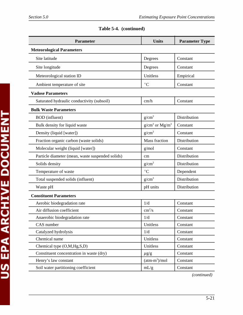
Table 5-4. (continued)
Section 5.0 Estimating Exposure Point Concentrations
Parameter Units Parameter Type
5-21
Meteorological Parameters
Site latitude Degrees Constant
Site longitude Degrees Constant
Meteorological station ID Unitless Empirical
Ambient temperature of site �C Constant
Vadose Parameters
Saturated hydraulic conductivity (subsoil) cm/h Constant
Bulk Waste Parameters
BOD (influent) g/cm3 Distribution
Bulk density for liquid waste g/cm3 or Mg/m3 Constant
Density (liquid [water]) g/cm3 Constant
Fraction organic carbon (waste solids) Mass fraction Distribution
Molecular weight (liquid [water]) g/mol Constant
Particle diameter (mean, waste suspended solids) cm Distribution
Solids density g/cm3 Distribution
Temperature of waste �C Dependent
Total suspended solids (influent) g/cm3 Distribution
Waste pH pH units Distribution
Constituent Parameters
Aerobic biodegradation rate 1/d Constant
Air diffusion coefficient cm2/s Constant
Anaerobic biodegradation rate 1/d Constant
CAS number Unitless Constant
Catalyzed hydrolysis 1/d Constant
Chemical name Unitless Constant
Chemical type (O,M,Hg,S,D) Unitless Constant
Constituent concentration in waste (dry) µg/g Constant
Henry’s law constant (atm-m3)/mol Constant
Soil water partitioning coefficient mL/g Constant
(continued)
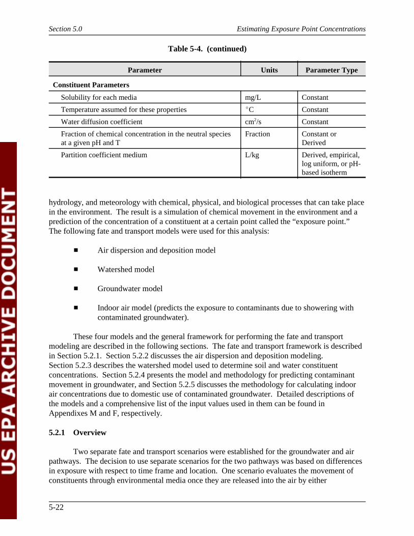
Table 5-4. (continued)
Section 5.0 Estimating Exposure Point Concentrations
Parameter Units Parameter Type
5-22
Constituent Parameters
Solubility for each media mg/L Constant
Temperature assumed for these properties �C Constant
Water diffusion coefficient cm2/s Constant
Fraction of chemical concentration in the neutral speciesat a given pH and T
Fraction Constant orDerived
Partition coefficient medium L/kg Derived, empirical,log uniform, or pH-based isotherm
hydrology, and meteorology with chemical, physical, and biological processes that can take placein the environment. The result is a simulation of chemical movement in the environment and aprediction of the concentration of a constituent at a certain point called the “exposure point.” The following fate and transport models were used for this analysis:
� Air dispersion and deposition model
� Watershed model
� Groundwater model
� Indoor air model (predicts the exposure to contaminants due to showering withcontaminated groundwater).
These four models and the general framework for performing the fate and transportmodeling are described in the following sections. The fate and transport framework is describedin Section 5.2.1. Section 5.2.2 discusses the air dispersion and deposition modeling. Section 5.2.3 describes the watershed model used to determine soil and water constituentconcentrations. Section 5.2.4 presents the model and methodology for predicting contaminantmovement in groundwater, and Section 5.2.5 discusses the methodology for calculating indoorair concentrations due to domestic use of contaminated groundwater. Detailed descriptions ofthe models and a comprehensive list of the input values used in them can be found inAppendixes M and F, respectively.
5.2.1 Overview
Two separate fate and transport scenarios were established for the groundwater and airpathways. The decision to use separate scenarios for the two pathways was based on differencesin exposure with respect to time frame and location. One scenario evaluates the movement ofconstituents through environmental media once they are released into the air by either
Section 5.0 Estimating Exposure Point Concentrations
5-23
volatilization or particulate release from the waste management unit. The second scenarioconsiders the movement of the constituent through soils and the groundwater once it has leachedfrom the bottom of a WMU. Environmental contamination from air releases can occurimmediately while it may take hundreds of years for most contaminants to reach a groundwaterwell; thus, for most contaminants, the exposure point concentrations predicted did not includesimultaneous contributions from both air and groundwater scenarios. In addition, theaboveground receptor locations may not necessarily overlap (i.e., the aboveground receptors arerandomly located around the WMU and may not coincide with the location of the groundwaterplume).
Both the groundwater and the air pathway modeling were designed to predict exposurepoint concentrations with which a resident living in the vicinity of the WMU may come intocontact during normal daily activities. For example, the air pathway analysis evaluatesconstituent concentrations in aboveground environmental media (e.g., air, soil, surface water). Aboveground constituent concentrations enter the human food chain via farm food commoditiesand fish. These farm food chain and aquatic food chain calculations are discussed in Section 5.3. The groundwater pathway analysis estimates the concentration of a constituent that may bepresent in a resident’s drinking water and indoor environment.
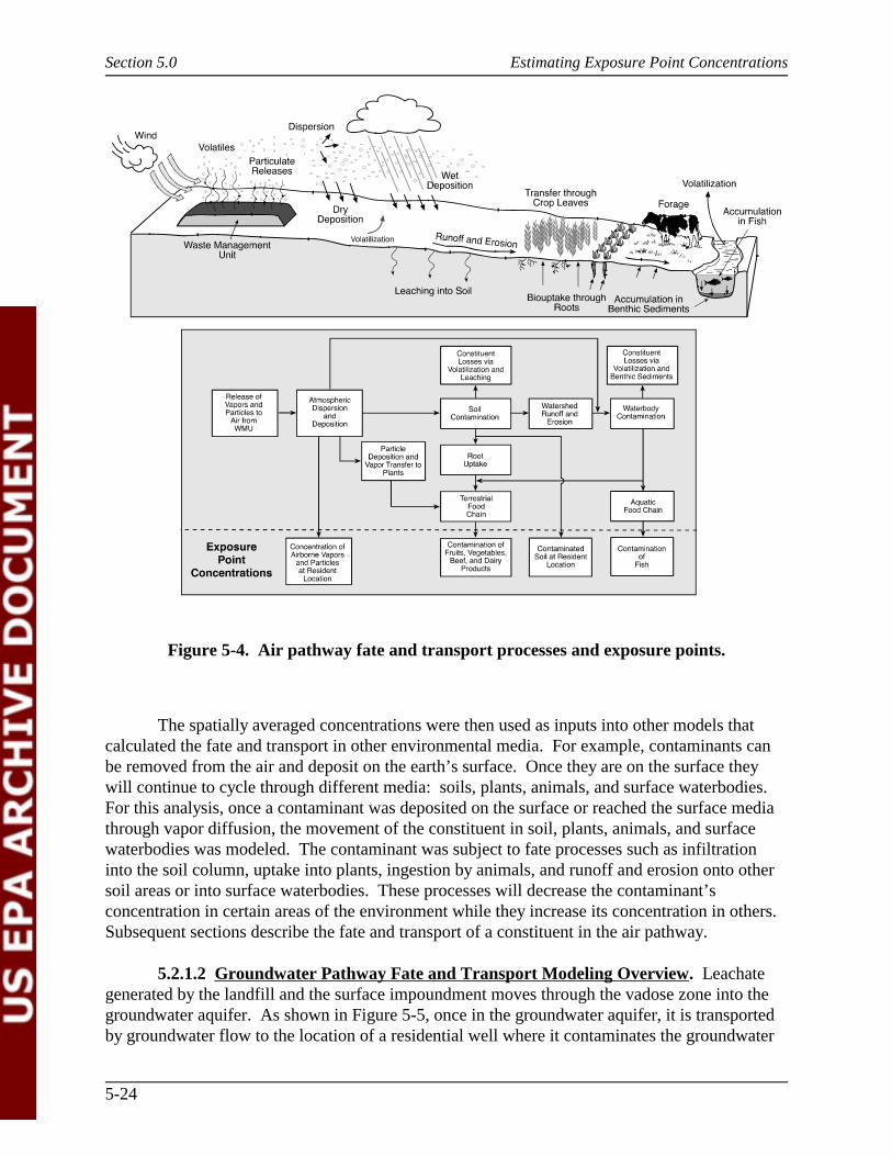
5.2.1.1 Air Pathway Fate and Transport Modeling Overview. Constituents releasedfrom a WMU either by volatilization of vapors or wind erosion of particulates will travel throughthe ambient air as a result of air movement. Wind direction and speed will determine how far theconstituent travels from the original source of its release. As shown in Figure 5-4, constituentstransported through the air can move through many different media: soil, biota, and surfacewaters. Initially, the wind will disperse the constituent in three dimensions. Due to the forces ofgravity and scavenging (mechanism by which constituents are removed from the air by cominginto contact with stationary objects, such as trees or by precipitation), the constituent may moveout of the ambient air onto plant, soils, or surface waterbodies. The constituent will thencontinue to move once it has deposited on these areas. For example, precipitation may inducerunoff and erosion onto other soils or into surface waters. All of these mechanisms will impactthe final concentration at an exposure point. For the air pathway, exposure point concentrationswere determined in
� Ambient air� Soils� Terrestrial food chain� Aquatic food chain.
To obtain these exposure point concentrations, air dispersion modeling was used topredict ambient air concentrations and the deposition fluxes of the released constituents. The airconcentrations and deposition values predicted were then input into a geographic informationsystem. The GIS was used to integrate the air modeling data over the spatial extent of thegeographic features in the study area. For example, the GIS was used to determine the averageair concentration over geographic features such as an agricultural field or waterbody. This spatialintegration produced normalized, spatially averaged air concentrations and deposition fluxes forareas adjacent to the WMU.
Section 5.0 Estimating Exposure Point Concentrations
5-24
Figure 5-4. Air pathway fate and transport processes and exposure points.
The spatially averaged concentrations were then used as inputs into other models thatcalculated the fate and transport in other environmental media. For example, contaminants canbe removed from the air and deposit on the earth’s surface. Once they are on the surface theywill continue to cycle through different media: soils, plants, animals, and surface waterbodies. For this analysis, once a contaminant was deposited on the surface or reached the surface mediathrough vapor diffusion, the movement of the constituent in soil, plants, animals, and surfacewaterbodies was modeled. The contaminant was subject to fate processes such as infiltrationinto the soil column, uptake into plants, ingestion by animals, and runoff and erosion onto othersoil areas or into surface waterbodies. These processes will decrease the contaminant’sconcentration in certain areas of the environment while they increase its concentration in others. Subsequent sections describe the fate and transport of a constituent in the air pathway.
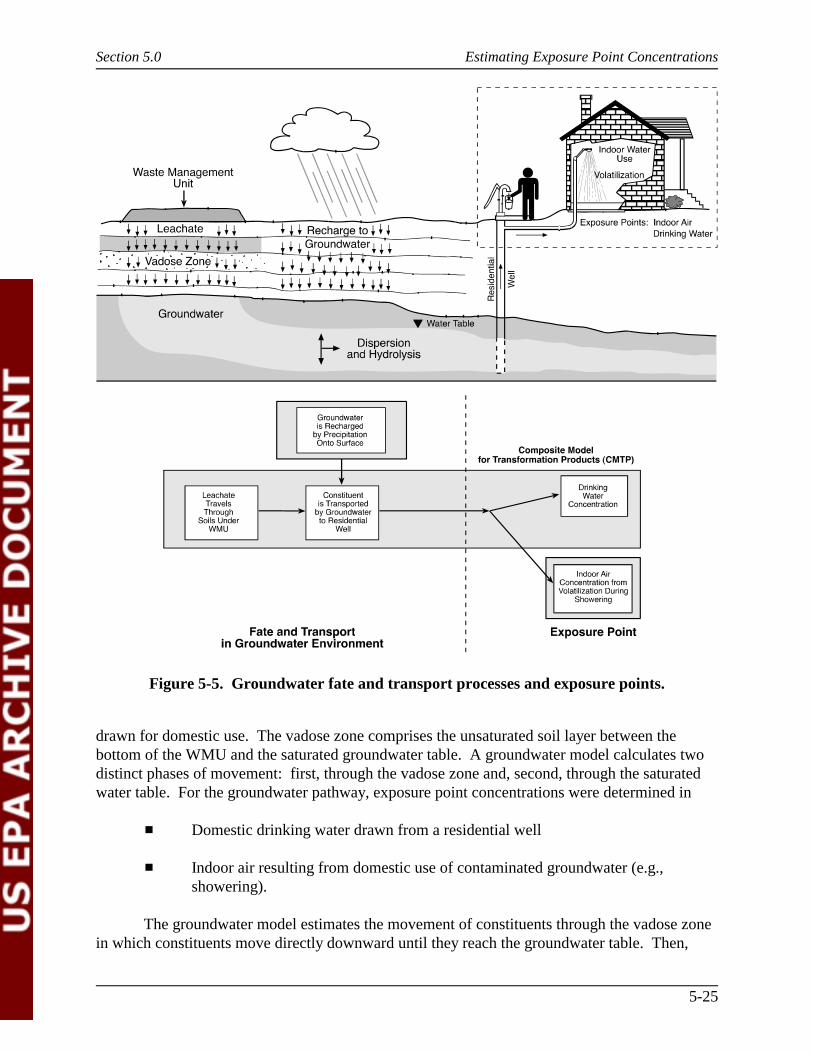
5.2.1.2 Groundwater Pathway Fate and Transport Modeling Overview. Leachategenerated by the landfill and the surface impoundment moves through the vadose zone into thegroundwater aquifer. As shown in Figure 5-5, once in the groundwater aquifer, it is transportedby groundwater flow to the location of a residential well where it contaminates the groundwater
Section 5.0 Estimating Exposure Point Concentrations
5-25
Figure 5-5. Groundwater fate and transport processes and exposure points.
drawn for domestic use. The vadose zone comprises the unsaturated soil layer between thebottom of the WMU and the saturated groundwater table. A groundwater model calculates twodistinct phases of movement: first, through the vadose zone and, second, through the saturatedwater table. For the groundwater pathway, exposure point concentrations were determined in
� Domestic drinking water drawn from a residential well
� Indoor air resulting from domestic use of contaminated groundwater (e.g.,showering).
The groundwater model estimates the movement of constituents through the vadose zonein which constituents move directly downward until they reach the groundwater table. Then,
Section 5.0 Estimating Exposure Point Concentrations
5-26
transport of constituents from the WMU to a residential well located downgradient of the WMUis modeled. Modeling constituent movement through the saturated groundwater takes intoaccount transport and dispersion of constituent by the water moving through the saturatedgroundwater table. Time of transport through the groundwater aquifer may be hundreds of years,during which chemical processes (e.g., hydrolysis) also break down the constituent. The result ofthese calculations is a dilution attenuation factor (DAF) for chemical constituents. The DAF isthe ratio of constituent concentration in the leachate released from the WMU to constituentconcentration in the groundwater at the location of the residential well. These DAFs were usedto relate constituent concentration at a residential well to leachate concentrations at the landfilland surface impoundment. The well water concentration was used to evaluate residentialdrinking water exposure and indoor air exposure due to indoor water use (e.g., showering). Thegroundwater pathway was evaluated separately from the air pathway in this assessment becausethe time frame and receptor locations for these two routes of exposure do not necessarilycoincide.
5.2.2 Dispersion and Deposition Modeling
Dispersion modeling is a computer-based set of calculations used to estimate ambientground-level constituent concentrations associated with constituent releases from a WMU. Thedispersion model uses information on meteorology (e.g., windspeed and direction, temperature)to estimate the movement of constituents through the atmosphere. Movement downwind islargely determined by windspeed and direction. Dispersion around the centerline of thecontaminant plume is estimated by empirically derived dispersion coefficients that account formovement of constituents in the horizontal and vertical directions. In addition, constituentmovement from the atmosphere to the ground is also modeled to account for depositionprocesses driven by gravitational settling and removal by precipitation.
The air dispersion and deposition modeling conducted for this analysis produced outputfiles of data that were used to calculate environmental media concentrations and food chainconcentrations (see Section 5.3). The dispersion model outputs included air concentration ofvapors and particles, wet deposition of vapors and particles, and dry deposition of particles. Drydeposition of vapors was also calculated but outside the dispersion model.
5.2.2.1 Industrial Source Complex Short Term Dispersion Model. A number ofdispersion models are available for estimating the transport of constituent through theatmosphere, several of which are available on EPA’s Support Center for Regulatory Air Models(SCRAM) Bulletin Board (http://www.epa.gov/scram001/). These dispersion models weredeveloped for a variety of applications and each has its own strengths and weaknesses. TheIndustrial Source Complex Short Term, Version 3 (ISCST3) model was selected for airdispersion modeling in this analysis. Because this assessment required a model with thecapability to model area sources, ground-level and elevated sources, ambient air concentrationsand deposition fluxes, vapors and particulates, and annual averaging times, ISCST3 was anappropriate model to use. In addition, ISCST3 has been supported by EPA’s Office of AirQuality Planning and Standards and has been used extensively in regulatory applications.
Section 5.0 Estimating Exposure Point Concentrations
5-27
ISCST3 (U.S. EPA, 1999a), a recommended dispersion model in EPA’s Guideline on AirQuality Models (U.S. EPA, 1999c), is a steady-state, Gaussian plume dispersion model. Asteady-state model is one in which the model inputs and outputs are constant with respect totime. That is, the system being modeled is assumed to be unchanging over time. The termGaussian plume refers to the kind of mathematical solution used to solve the air dispersionequations. It essentially means that the constituent concentration is dispersed within the plumelaterally and vertically according to a Gaussian distribution, which is similar to a normaldistribution. These assumptions and solutions hold for each hour modeled. The results for eachhour are then processed to provide values for different averaging times depending on the user’sneeds (e.g., annual average).
ISCST3 is capable of simulating dispersion of pollutants from a variety of sources,including point, area, volume, and line sources. ISCST3 can account for both long- and short-term air concentration of particles and vapor and wet and dry deposition of particles and vapor. In addition to deposition, wet and dry plume depletion can be selected to account for removal ofmatter by deposition processes and to maintain mass balance. Receptors can be specified inpolar or cartesian arrays or can be set to discrete points as needed. Flat or rolling terrain may bemodeled but only flat terrain may be used for area sources. ISCST3 considers effects ondispersion of environmental setting by allowing the user to set urban or rural dispersionparameters.
5.2.2.2 Configuration of ISCST3 for Air Dispersion and Deposition Modeling. Results of air dispersion and deposition modeling represent the initial step in the fate andtransport of vapor and particle emissions in the environment. The ISCST3 model was used toestimate the
� Air concentration of vapors� Air concentration of particles� Wet deposition of vapors and particles� Dry deposition of particles onto soils.
Dry deposition of vapors was calculated outside of ISCST3 as explained below.
All air concentrations and deposition values developed by ISCST3 were unit values basedon modeling default unit emission rates. For treatment tank modeling, the default unit emissionapplied was 1 g/s-m2. This unit emission rate resulted in unit air concentrations measured in(µg/m3) per (unit emission rate of 1 g/s-m2) and deposition rates measured in (g/m2) per (unitemission rate of 1 g/s-m2). Due to the large range of surface areas being considered for landfillsand surface impoundments, modeling of these units required the use of two different unitemission rates. That is, a unit emission rate of 1 µg/s-m2 was applied for sources larger than5,000 m2, and 1 mg/s-m2 was applied for sources 5,000 m2 and smaller. External to ISCST3, theresulting unit concentrations and deposition rates were adjusted by applying the appropriatemultipliers (1E+06 g/µg and 1E+03 g/mg). Later in the exposure modeling process, the unit airconcentrations [(µg/m3) per (unit emission rate of 1 g/s-m2)] and deposition rates [(g/m2) per(unit emission rate of 1 g/ s-m2)] were multiplied by chemical-specific emission rates to producevalues used to calculate environmental media concentrations.
Section 5.0 Estimating Exposure Point Concentrations
5-28
Assumptions Made for ISCST3 Modeling
� Wet and dry depletion were activated in thedispersion modeling for particles. Wet depletion wasconsidered for vapors.
� Area source was modeled for all WMUs.
� To minimize error due to site orientation, circular areasources centered on the origin were modeled.
� Modeling was conducted using unit emission rates.
� Receptors were placed on receptor rings ranging from0 to 2,000 m starting from the edge of the source with16 receptor points on each ring.
� The rural option was used in the ISCST3 modelingsince the types of WMUs being assessed are typicallyin nonurban areas.
� Flat terrain was assumed.
Modeling was conducted using 5 years of data obtained from 49 representativemeteorological stations throughout the country (see Section 4.3 for a discussion ofmeteorological site selection). Modeling was conducted for many separate scenarios designed tocover a broad range of WMU characteristics, including
� Ground-level and elevated sources
� 21 surface area sizes for landfills, 20 area sizes for surface impoundments, and31 area-height combinations for tanks
� Distances ranging from 0 to 2,000 m from the WMU placed in 16 directionsspaced every 22.5 degrees around the circumference of the WMU.
Air Concentrations of Vapor and Particles. ISCST3 estimates air concentrations of
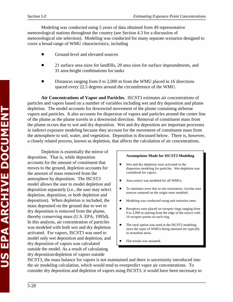
particles and vapors based on a number of variables including wet and dry deposition and plumedepletion. The model accounts for downwind movement of the plume containing airbornevapors and particles. It also accounts for dispersion of vapors and particles around the center lineof the plume as the plume travels in a downwind direction. Removal of constituent mass fromthe plume occurs due to wet and dry deposition. Wet and dry deposition are important processesin indirect exposure modeling because they account for the movement of constituent mass fromthe atmosphere to soil, water, and vegetation. Deposition is discussed below. There is, however,a closely related process, known as depletion, that affects the calculation of air concentrations.
Depletion is essentially the mirror ofdeposition. That is, while depositionaccounts for the amount of constituent thatmoves to the ground, depletion accounts forthe amount of mass removed from theatmosphere by deposition. The ISCST3model allows the user to model depletion anddeposition separately (i.e., the user may selectdepletion, deposition, or both depletion anddeposition). When depletion is included, themass deposited on the ground due to wet ordry deposition is removed from the plume,thereby conserving mass (U.S. EPA, 1995d). In this analysis, air concentration of particleswas modeled with both wet and dry depletionactivated. For vapors, ISCST3 was used tomodel only wet deposition and depletion, anddry deposition of vapors was calculatedoutside the model. As a result of calculatingdry deposition/depletion of vapors outsideISCST3, the mass balance for vapors is not maintained and there is uncertainty introduced intothe air modeling calculation, which would tend to overpredict vapor air concentrations. Toconsider dry deposition and depletion of vapors using ISCST3, it would have been necessary to

Section 5.0 Estimating Exposure Point Concentrations
1 Koester and Hites (1992) suggest that the dry deposition of vapor may be negligible.
5-29
provide chemical-specific gas deposition information, which is not readily available. Furthermore, it would have been necessary to conduct chemical-specific modeling, significantlyincreasing the number of air dispersion model runs needed.
Wet Deposition of Particles and Vapor. Wet deposition is the deposition of material ona surface from a plume as a result of precipitation. The amount of material removed by wetdeposition from the plume is a function of the scavenging rate coefficient, which is based onparticle size (U.S. EPA, 1995d). To perform these calculations, wet deposition, wet depletion,and dry depletion were all selected in the input run-stream file. Precipitation data from the Solarand Meteorological Surface Observation Network (SAMSON) CD-ROM, (U.S. DOC and U.S.DOE, 1993) were required to process the meteorological inputs for this analysis.
Dry Deposition of Particles. Dry deposition refers to the deposition of material on asurface (e.g., ground, vegetation) from a plume of material as a result of processes such asgravitational settling, turbulent diffusion, and molecular diffusion. Dry deposition is calculatedas the product of air concentration and dry deposition velocity. To calculate dry deposition,ISCST3 requires mass mean diameter, particle density, and mass fraction to be input into thesource pathway for deposition calculations (U.S. EPA, 1995b). Dry deposition calculations alsorequire the meteorological input file to contain surface friction velocity, hourly Monin-Obukhovlength, and surface roughness length. Surface friction velocity and hourly Monin-Obukhovlength were calculated in the PCRAMMET preprocessor (U.S. EPA, 1995c). More detail on thePCRAMMET preprocessor is provided in Appendix N.
Dry Deposition of Vapors. Dry deposition of vapors was calculated using a stepexternal to the ISCST3 model because chemical-specific dry deposition modeling within ISCST3was precluded by time and resource considerations. Using a dry deposition algorithm forparticles (from the ISCST user’s manual), dry deposition of vapor was calculated by multiplyingthe vapor air concentration by a default deposition velocity of 0.2 cm/s (Koester and Hites,1992). This approach assumes that vapors behave as fine aerosols and, therefore, are amenableto modeling using the dry deposition algorithm for particles.1
To calculate the weighted dry deposition velocity, land use was obtained from 1:250,000-scale quadrangles of land use and GIRAS spatial data obtained from the EPA website and placedin an ARC-INFO format (U.S. EPA, 1994). Land use was based on data from the mid-1970s tothe early 1980s. The fraction of time in each stability class was based on 5-year hourlymeteorological files used in ISCST3 modeling.
Averaging Time. For the paints listing risk assessment, all human health and ecologicalrisks were evaluated based on benchmarks for chronic, long-term exposure. Therefore, the airconcentrations and deposition values required for the human health and ecological riskassessment were long-term averages. Long-term averages calculated by the ISCST3 model wereannual averages. However, since the ISCST3 model was run using 5 years of meteorologicaldata, it actually averages the hourly concentrations over the entire 5-year period.
Section 5.0 Estimating Exposure Point Concentrations
5-30
Rural vs. Urban. The rural vs. urban setting in ISCST3 allows the user to account fordifferences between rural and urban environments. In urban environments, the built environment(e.g., buildings, roads, and parking lots) alters the dispersion character of the atmosphere,particularly at night due to building-induced turbulence and reduced nighttime cooling. Thusthere is greater nighttime mixing of constituents in urban areas compared to rural areas. Forpurposes of ISCST3 modeling, the urban classification applies mainly to large cities; even smallcities and suburban areas are classified as rural for ISCST3 purposes. For this analysis, the ruralsetting was used because, although the specific location of the WMUs was not known, they arenot likely to be located within large cities.
Placements of Points Where Air Concentrations Were Calculated. A grid of pointswhere air concentration and deposition values were calculated was established using a polar grid.Air concentration and deposition values were produced for each point on the grid (i.e., x, ycoordinate) in a polar array consisting of 16 radials spaced every 22.50 degrees and rings atdistances ranging from 0 to 2,000 m from the edge of the WMU.
Flat vs. Elevated Terrain. The ISCST3 model allows the user to model to account forelevated terrain by specifying an elevation for each point on the grid where air concentrations anddeposition values are calculated. This feature, however, is not available for use with areasources. Because all sources modeled in this analysis were area sources, elevated terrain was notconsidered.
TOXIC vs. Regulatory Mode. The most recent version of ISCST3 (99155, U.S. EPA,1999a) allows the user to select a regulatory default option or to select a TOXICS option. Theregulatory default option uses Romberg numeric integration solution to estimate air concentrationfrom an area source. Based on the results of validation tests performed by EPA, EPA hasconcluded that the Romberg algorithm performs very well in terms of efficiency andreasonableness (U.S. EPA, 1992d). However, this algorithm takes a significant amount of timeto execute for large area sources. To improve model run times, the TOXICS option was addedby EPA to the area source model. The TOXICS option also uses a Romberg numeric integrationsolution to estimate air concentrations and deposition rates near the WMU. Farther from theWMU, however, the TOXICS option uses a two-point Gaussian Quadrature routine instead ofthe Romberg solution to estimate air concentration and deposition. The two-point GaussianQuadrature solution is computationally more efficient, which accounts for the shorter model runtime. For this study, a sensitivity analysis was conducted to compare the estimated airconcentrations calculated using the regulatory option to those calculated using the TOXICSmode. This analysis showed small differences between results obtained using either option (seeAppendix N). Given the benefit of reduced run times, the TOXICS option was selected in thisanalysis.
Source Shape. All WMU types modeled in this analysis were modeled as area sources. Landfills and surface impoundments were modeled as ground-level sources, and treatment tankswere modeled as elevated sources. The ISCST3 model allows the user to model area sources aspolygonal sources with from 3 to 20 sides (U.S. EPA, 1999a). The ISCST3 was set up in thisanalysis to model an area source as a 20-sided polygon shaped to approximate a circle. This
Section 5.0 Estimating Exposure Point Concentrations
5-31
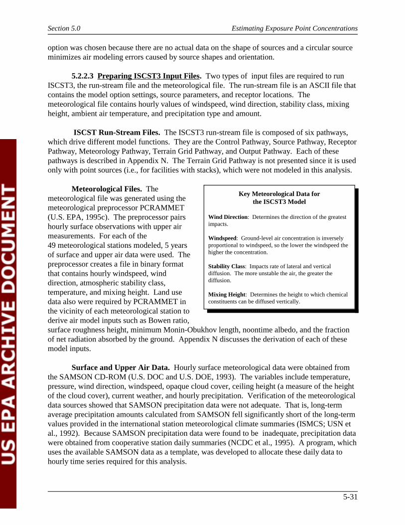
Key Meteorological Data for the ISCST3 Model
Wind Direction: Determines the direction of the greatestimpacts.
Windspeed: Ground-level air concentration is inverselyproportional to windspeed, so the lower the windspeed thehigher the concentration.
Stability Class: Impacts rate of lateral and verticaldiffusion. The more unstable the air, the greater thediffusion.
Mixing Height: Determines the height to which chemicalconstituents can be diffused vertically.
option was chosen because there are no actual data on the shape of sources and a circular sourceminimizes air modeling errors caused by source shapes and orientation.
5.2.2.3 Preparing ISCST3 Input Files. Two types of input files are required to runISCST3, the run-stream file and the meteorological file. The run-stream file is an ASCII file thatcontains the model option settings, source parameters, and receptor locations. Themeteorological file contains hourly values of windspeed, wind direction, stability class, mixingheight, ambient air temperature, and precipitation type and amount.
ISCST Run-Stream Files. The ISCST3 run-stream file is composed of six pathways,which drive different model functions. They are the Control Pathway, Source Pathway, ReceptorPathway, Meteorology Pathway, Terrain Grid Pathway, and Output Pathway. Each of thesepathways is described in Appendix N. The Terrain Grid Pathway is not presented since it is usedonly with point sources (i.e., for facilities with stacks), which were not modeled in this analysis.
Meteorological Files. Themeteorological file was generated using themeteorological preprocessor PCRAMMET (U.S. EPA, 1995c). The preprocessor pairshourly surface observations with upper airmeasurements. For each of the49 meteorological stations modeled, 5 yearsof surface and upper air data were used. Thepreprocessor creates a file in binary formatthat contains hourly windspeed, winddirection, atmospheric stability class,temperature, and mixing height. Land usedata also were required by PCRAMMET inthe vicinity of each meteorological station toderive air model inputs such as Bowen ratio,surface roughness height, minimum Monin-Obukhov length, noontime albedo, and the fractionof net radiation absorbed by the ground. Appendix N discusses the derivation of each of thesemodel inputs.
Surface and Upper Air Data. Hourly surface meteorological data were obtained fromthe SAMSON CD-ROM (U.S. DOC and U.S. DOE, 1993). The variables include temperature,pressure, wind direction, windspeed, opaque cloud cover, ceiling height (a measure of the heightof the cloud cover), current weather, and hourly precipitation. Verification of the meteorologicaldata sources showed that SAMSON precipitation data were not adequate. That is, long-termaverage precipitation amounts calculated from SAMSON fell significantly short of the long-termvalues provided in the international station meteorological climate summaries (ISMCS; USN etal., 1992). Because SAMSON precipitation data were found to be inadequate, precipitation datawere obtained from cooperative station daily summaries (NCDC et al., 1995). A program, whichuses the available SAMSON data as a template, was developed to allocate these daily data tohourly time series required for this analysis.

Section 5.0 Estimating Exposure Point Concentrations
5-32
Mixing heights were calculated using surface and upper air station data. The upper airdata were compiled from the Radiosonde Data of North America CD-ROM (NCDC, 1997). Mixing height is the height to which vertical dispersion of constituent can occur.
Filling Missing Data. Missing surface data were identified using a computer program tosearch for incidents of missing data on the observation indicator, opaque cloud cover,temperature, station pressure, wind direction and speed, and ceiling height. Missing surface datawere filled in by another computer program. This program fills in up to 5 consecutive hours ofdata for cloud cover, ceiling height, temperature, pressure, wind direction, and windspeed. Forsingle missing values, the program follows the objective procedures developed by Atkinson andLee (1992). For two to five consecutive missing values, other rules were developed because thesubjective methods provided by Atkinson and Lee (1992) rely on professional judgment andcould not be programmed. The program flagged files where missing data exceeded fiveconsecutive values. In the few cases where this occurred and the missing data did not constitute10 percent of the file, they were provided manually according to procedures set forth in Atkinsonand Lee (1992). Years that were missing 10 percent or more of the data were discarded(Atkinson and Lee, 1992). If a meteorological station did not have 5 years with sufficient datacompleteness, the station was discarded and another station was selected.
5.2.2.4 Source Areas Modeled. In the modeling analysis, three types of WMUs wereconsidered (i.e., landfill, treatment tanks, and surface impoundments). Because the ISCST3model is sensitive to the size of the area source, the relationship between air concentrations andsize of the area source was analyzed. As illustrated in Figure 5-6, the results show that, forrelatively small area sources, air concentrations increase significantly as the size of the areasource increases. For large area sources, this increase in air concentrations is not as significant.
To address this model sensitivity yet avoid modeling over 2,800 separate WMUs, area-based strata that represent the distribution of surface areas for each of the WMU types weredeveloped. Landfills and surface impoundment units were modeled as ground-level area sources,and tanks were modeled as elevated area sources. Separate strata were developed for each WMUtype. The sampling of WMUs and the creation of strata to represent the distribution ofdimensions found in the underlying databases are discussed in Section 4.4. In that section, thesource areas and heights used in the modeling analysis are presented.
For each WMU type, the median area for each strata were input into ISCST and modeledfor each of the 49 meteorological stations. For tanks, each area-height combination was modeledfor each of the 49 meteorological locations. This provided a set of unit air concentrations for usein the analysis. For any specific WMU, the median unit air concentration and deposition valuesfor the strata were used to represent all WMUs from that strata. The strata were designed to benarrower for the smaller areas because this is where air concentrations have the greatest rate ofchange with respect to change in area. This minimizes the error associated with not modelingeach individual WMU.
5.2.2.5 Spatial Averaging of Air Concentrations and Deposition. A GIS model wasused to calculate air concentration and deposition rates for the resident location, buffer area,agricultural field, and waterbodies. This crucial step combines the spatial characterization of the
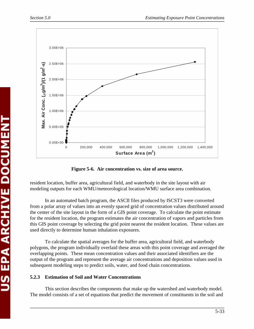
Section 5.0 Estimating Exposure Point Concentrations
5-33
0.00E+00
5.00E+05
1.00E+06
1.50E+06
2.00E+06
2.50E+06
3.00E+06
0 200,000 400,000 600,000 800,000 1,000,000 1,200,000 1,400,000
Surface Area (m2)
Max
. Air
Co
nc.
( �
g/m
3)/
(1 g
/m2-s
)
Figure 5-6. Air concentration vs. size of area source.
resident location, buffer area, agricultural field, and waterbody in the site layout with airmodeling outputs for each WMU/meteorological location/WMU surface area combination.
In an automated batch program, the ASCII files produced by ISCST3 were convertedfrom a polar array of values into an evenly spaced grid of concentration values distributed aroundthe center of the site layout in the form of a GIS point coverage. To calculate the point estimatefor the resident location, the program estimates the air concentration of vapors and particles fromthis GIS point coverage by selecting the grid point nearest the resident location. These values areused directly to determine human inhalation exposures.
To calculate the spatial averages for the buffer area, agricultural field, and waterbodypolygons, the program individually overlaid these areas with this point coverage and averaged theoverlapping points. These mean concentration values and their associated identifiers are theoutput of the program and represent the average air concentrations and deposition values used insubsequent modeling steps to predict soils, water, and food chain concentrations.
5.2.3 Estimation of Soil and Water Concentrations
This section describes the components that make up the watershed and waterbody model. The model consists of a set of equations that predict the movement of constituents in the soil and
Section 5.0 Estimating Exposure Point Concentrations
5-34
a set of equations that determine the fate of constituents in a surface waterbody. The output ofthese models provides the concentration of the constituent for the
� First 20 cm of soil� First 1 cm of soil� Dissolved water portion of the waterbody� Suspended solids portion of the waterbody� Benthic sediment portion of the waterbody� Benthic sediment pore water portion of the waterbody.
Discussions in this section are general in nature. Two appendixes support the discussions withmore detailed information: Appendix M contains the full set of equations used to calculatemedia concentrations, and Appendix F lists the physical/chemical properties used; the parametervalues selected for fate, transport, and exposure modeling; and citations for the parameter valuesselected.
5.2.3.1 Predicting Soil Concentrations. Soil concentrations in a watershed werecalculated for both the buffer area and agricultural field. For this analysis, it is assumed thatconstituents deposited on buffer area soils adjacent to the WMU via air dispersion and depositionare subject to transport by erosion and runoff to the agricultural field. The concentration of aconstituent in soil is a function of what has been deposited onto the soil from the air and what hasbeen transported overland by erosion and runoff from adjacent land areas minus soil losses. Soillosses accounted for in this analysis include biodegradation, volatilization, leaching, surfacerunoff, and erosion. The following sections describe how each of these addition and removalmechanisms are estimated to obtain an overall soil concentration.
Characterization of location-specific meteorological factors (e.g., precipitation, irrigation,runoff, and evapotranspiration) and soils is important in predicting soil concentrations. Location-dependent meteorological factors and soil characteristics were taken from several sources and aredescribed in Section 4.3.
Addition of Constituents to Soils. Addition of constituents to soils, also calledconstituent loading, can result from atmospheric deposition and overland movement ofconstituents. Constituent loadings to the soil were calculated using equations presented in TablesM.2-2 and M.2-3 in Appendix M.
The primary loading mechanism is by wet and dry deposition of constituents from the airto the ground. Constituent deposition was predicted based on the average air concentration anddeposition flux for both the buffer area and the agricultural field. These mechanisms include wetdeposition of vapors and particles and dry deposition of vapors and particles.
There is no direct overland movement of constituents from the WMU to the buffer oragricultural field. However, loading due to overland transport from the buffer to the agriculturalfield can occur given that the buffer is contaminated due to direct deposition. The same erosionand runoff terms used to estimate loading from soils into the waterbodies are used to estimateloading from the buffer onto the agricultural field.
Section 5.0 Estimating Exposure Point Concentrations
5-35
Soil concentration due to loading from both overland transport and direct deposition isdependent on the depth of the soil column into which the constituent is mixed. The mixing depthin the soil (z) depends on whether the soil is disturbed by agricultural tilling. In this analysis, 20cm was used as the mixing depth for tilled soils and 1 cm was used for untilled soils(U.S. EPA, 1993). The soil bulk density converts a deposition rate from grams of contaminantper unit area to grams of contaminant per kilogram of soil.
Losses from Soils. Constituent losses from the soil were calculated using equationspresented in Tables M.2-4 through M.2-8 in Appendix M. Soil concentrations are calculatedusing a total loss term that represents total losses due to five separate processes:
� Leaching of the chemical into the groundwater due to precipitation� Erosion of the chemical laterally along with the soil due to water� Runoff of the dissolved chemical with the lateral flow of water� Biodegradation of the chemical in situ� Volatilization losses of the chemical.
The total loss term provides one overall loss constant that is applied in the calculation of soilconcentrations. The loss constant is applied over the same time period of constituent loading(i.e., the time period of deposition) during the operating life of the WMU. Each component ofthe total loss term is discussed below.
The leaching loss constant representing the rate at which constituents leach from soil is achemical-specific value that is a function of location-specific precipitation, irrigation, runoff, andevapotranspiration. The equation for calculating the leaching loss constant, ksl, is as shown inTable M.2-5 in Appendix M.
The Universal Soil Loss Equation was used to estimate soil erosion losses (Xe) as shownin Table M.2-8 in Appendix M. USLE is an empirically derived equation originally developedby the Soil Conservation Service of the U.S. Department of Agriculture to estimate soil erosionlosses from agricultural fields during soil conservation planning. The USLE is applied in thecontext of the Gross Erosion Sediment-Delivery Ratio method outlined in USDA (1978) anddescribed in greater detail in the SCS National Engineering Handbook (USDA, 1971). Grosserosion is defined as the summation of erosion from all sources within a watershed, as estimatedfor sheet and rill erosion by USLE. The sediment delivery ratio adjusts gross erosion rates toaccount for terrain and cover features, which effectively reduce sediment erosion.
The loss constant due to surface runoff was calculated as a function of chemical-specificvalues and location-specific average annual runoff, as shown in Table M.2-10 in Appendix M.
In this analysis, biodegradation losses from soil were considered for all organicchemicals. The vast majority of soil biodegradation rates were taken from Handbook ofEnvironmental Degradation Rates (Howard et al., 1991). The Handbook provides chemical-specific values for the half-life in soil. The highest half-life was used to derive degradation ratesince a higher half-life results in a lower degradation rate. A single biodegradation rate was usedfor each constituent. This biodegradation rate was applied to all WMUs in all locations. Site-

Section 5.0 Estimating Exposure Point Concentrations
5-36
specific conditions may cause the biodegradation rate to be greater or less than the default valueused, but this variability was not captured by this analysis.
The volatilization loss constant calculates the contaminant loss due to volatilization fromsoil. The calculation of the volatilization loss factor, ksv, is shown in Table M.2-11 inAppendix M. Volatilization kinetics are driven by chemical-specific properties andenvironmental conditions, including location-specific properties. Constituent properties thatinfluence volatilization include Henry’s law constant, the soil-water partitioning coefficient, andthe diffusivity in air. Volatilization is further influenced by environmental conditions includingsoil mixing depth, soil bulk density, ambient air temperature, average annual windspeed, andimpacted surface area. In this assessment, location-specific values were used for the ambient airtemperature and the average annual windspeed.
Calculation of Soil Concentrations. Following calculation of the constituent loadingrates and the rate loss constants, soil concentrations were estimated. Equations presented inTable M.2-1 in Appendix M were used to estimate soil concentrations.
Soil constituent concentration changes with each year of operation of a facility. Duringthe 30-year period for landfills or 50-year period for tanks and surface impoundments in which aWMU is assumed to operate, the constituent concentration in soil will steadily increase. Toaccount for this phenomenon, the equation to calculate average soil concentration over the timeperiod of deposition (facility operation) explicitly considers the time period of exposure for thereceptor of interest. This is accomplished by accounting for total loading and loss for each yearand then determining an average soil concentration.
For evaluating cancer risks, soil concentrations were explicitly averaged over theexposure period for the specific human receptor. This was accomplished using two timemeasures: the time period over which deposition occurs (i.e., the operating period of the WMU)and exposure duration. For exposure duration less than the operating period of the WMU, theaverage soil concentration is determined by the average of the last years of operation where thenumber of years integrated is equal to the exposure duration. During this period, soilconcentration is steadily increasing. For exposure durations greater than the operating period ofthe WMU, the soil concentrations are integrated over two periods. First, for the period spanningthe entire operating period of the WMU, soil concentrations are steadily increasing. Second, forthe period of time after the operating period of the WMU, soil concentration will be steadilydeclining. Since exposure duration is limited to 50 years, the scenarios in which the exposureduration is greater than the operating period of the WMU can only occur for landfills.
To evaluate noncancer effects from chemicals, soil concentrations were used for the timecorresponding to the end of the WMU operating period (i.e., 30 or 50 years). This is becauseless-than-lifetime average exposures are of interest for evaluating the potential for noncancereffects, such as developmental toxicity. Many chemicals will have reached steady-state wellbefore year 30 (or 50 depending on the WMU type). However, other chemicals will tend to buildup in soils for much longer periods. Limiting the soil concentrations to the operating period ofthe WMU represents a balance between the period of facility operating (which is uncertain) and ashorter time period (which could underestimate exposure from soil). Ecotoxicological risks were
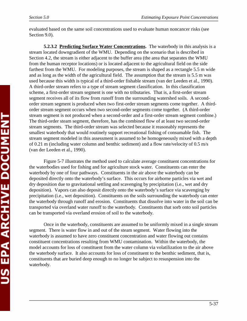
Section 5.0 Estimating Exposure Point Concentrations
5-37
evaluated based on the same soil concentrations used to evaluate human noncancer risks (seeSection 9.0).
5.2.3.2 Predicting Surface Water Concentrations. The waterbody in this analysis is astream located downgradient of the WMU. Depending on the scenario that is described inSection 4.2, the stream is either adjacent to the buffer area (the area that separates the WMUfrom the human receptor locations) or is located adjacent to the agricultural field on the sidefarthest from the WMU. For modeling purposes, the stream is shaped as a rectangle 5.5 m wideand as long as the width of the agricultural field. The assumption that the stream is 5.5 m wasused because this width is typical of a third-order fishable stream (van der Leeden et al., 1990). A third-order stream refers to a type of stream segment classification. In this classificationscheme, a first-order stream segment is one with no tributaries. That is, a first-order streamsegment receives all of its flow from runoff from the surrounding watershed soils. A second-order stream segment is produced when two first-order stream segments come together. A third-order stream segment occurs when two second-order segments come together. (A third-orderstream segment is not produced when a second-order and a first-order stream segment combine.) The third-order steam segment, therefore, has the combined flow of at least two second-orderstream segments. The third-order stream was selected because it reasonably represents thesmallest waterbody that would routinely support recreational fishing of consumable fish. Thestream segment modeled in this assessment is assumed to be homogeneously mixed with a depthof 0.21 m (including water column and benthic sediment) and a flow rate/velocity of 0.5 m/s(van der Leeden et al., 1990).
Figure 5-7 illustrates the method used to calculate average constituent concentrations forthe waterbodies used for fishing and for agriculture stock water. Constituents can enter thewaterbody by one of four pathways. Constituents in the air above the waterbody can bedeposited directly onto the waterbody’s surface. This occurs for airborne particles via wet anddry deposition due to gravitational settling and scavenging by precipitation (i.e., wet and drydeposition). Vapors can also deposit directly onto the waterbody’s surface via scavenging byprecipitation (i.e., wet deposition). Constituents on the soils surrounding the waterbody can enterthe waterbody through runoff and erosion. Constituents that dissolve into water in the soil can betransported via overland water runoff to the waterbody. Constituents that sorb onto soil particlescan be transported via overland erosion of soil to the waterbody.
Once in the waterbody, constituents are assumed to be uniformly mixed in a single streamsegment. There is water flow in and out of the steam segment. Water flowing into thewaterbody is assumed to have zero constituent concentration and water flowing out containsconstituent concentrations resulting from WMU contamination. Within the waterbody, themodel accounts for loss of constituent from the water column via volatilization to the air abovethe waterbody surface. It also accounts for loss of constituent to the benthic sediment, that is,constituents that are buried deep enough to no longer be subject to resuspension into thewaterbody.
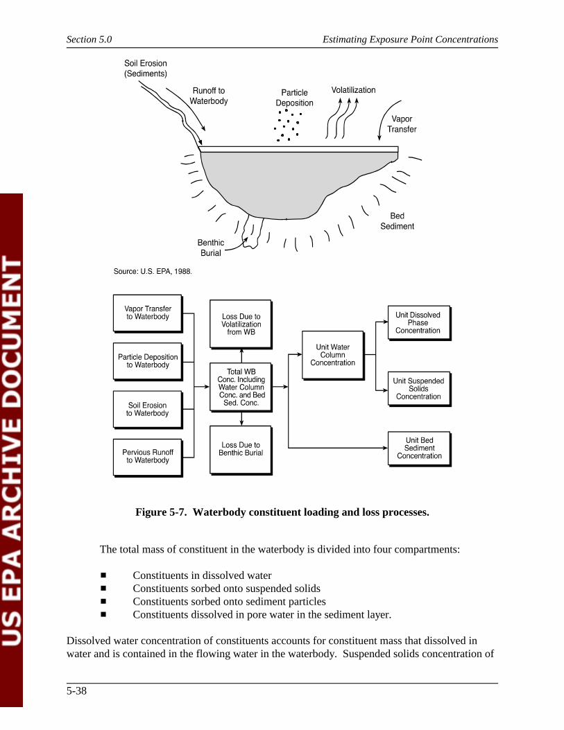
Section 5.0 Estimating Exposure Point Concentrations
5-38
Figure 5-7. Waterbody constituent loading and loss processes.
The total mass of constituent in the waterbody is divided into four compartments:
� Constituents in dissolved water� Constituents sorbed onto suspended solids� Constituents sorbed onto sediment particles� Constituents dissolved in pore water in the sediment layer.
Dissolved water concentration of constituents accounts for constituent mass that dissolved inwater and is contained in the flowing water in the waterbody. Suspended solids concentration of
Section 5.0 Estimating Exposure Point Concentrations
5-39
constituents accounts for constituent mass that is sorbed onto particles that are suspended in theflowing water in the waterbody. Sediment constituent concentrations account for constituentmass that is sorbed onto particles that settle to the sediment layer at the bottom of the waterbody. Pore water constituent concentrations account for constituent mass that is dissolved in the watercontained in the pore spaces in the sediment layer.
Humans and wildlife are exposed to constituents in these various waterbodycompartments depending on the route of exposure. For example, one waterbody is used fordrinking water for beef cattle and dairy cows. Because these animals drink water directly fromthe waterbody (i.e., the water is not filtered), their exposure to constituents from drinking stockwater comes from both dissolved and suspended constituent concentrations. Section 5.3describes the calculation of farm food chain and aquatic food chain concentrations in greaterdetail. Section 9.0 describes ecological exposures that, in part, are based on waterbodyconcentrations.
Loading to a Waterbody. There are four ways a constituent may enter the waterbody:
� Constituents may be bound to airborne particles that are deposited on thewaterbody surface (e.g., wet and dry deposition of particles)
� Vapor phase constituents in the air may transfer to the surface waterbody (e.g.,wet and dry deposition of vapors)
� Constituents may be dissolved in runoff that enters the surface waterbody
� Constituents may be sorbed to eroded soil particles that enter the surfacewaterbody.
These concentrations were predicted using the results of air modeling and soil calculationsdescribed in Sections 5.2.2 and 5.3.1, respectively. Equations describing how the modelcalculates these loadings are provided in Tables M.3-4 through M.3-8 in Appendix M.
Constituent Losses from Surface Waterbody. Constituent losses due to volatilizationand burial in benthic sediments were considered. After accounting for the losses, the totalwaterbody concentration was apportioned to the water column and bed sediments irrespective ofthe loss mechanism. Therefore, at equilibrium, both loss mechanisms affect both compartmentsto the same extent. The two divisions of the total waterbody concentration (into the watercolumn concentration and the bed sediment concentration) were further divided chemicallybetween the fraction that is sorbed to sediments and suspended solids and the fraction that isdissolved. Equations describing how the model calculates these losses are provided inTables M.3-9 through M.3-11 in Appendix M.
Calculating Surface Water and Sediment Concentrations. Following calculation ofthe constituent loading and loss rates, waterbody constituent concentrations were estimated usingequations presented in Table M.3-3 in Appendix M.
Section 5.0 Estimating Exposure Point Concentrations
5-40
As discussed in Section 5.2.3.1, watershed soil constituent concentration changes witheach year of operation of a facility. To account for this phenomenon, soil concentrations werecalculated over the time period of deposition (facility operation), and the time period of exposurefor the receptor of interest was explicitly considered. This time-averaged soil concentration isreflected in the calculation of waterbody concentrations. The waterbody model is a steady-statemodel; that is, all inputs and outputs from the waterbody system are assumed to be unchangingwith time. Therefore, the soil concentrations were calculated outside the waterbody model andinput to the model as constant rates reflecting different exposure scenarios and receptors.
For evaluating cancer risks, waterbody loadings were calculated using soil concentrationsthat were explicitly averaged over the exposure period for the specific human receptor asdiscussed in Section 5.2.3.1. To evaluate noncancer effects from chemicals, waterbodyconcentrations were calculated using soil concentrations calculated for the time periodcorresponding to the end of the WMU operating period (i.e., 30 years for landfills or 50 years fortreatment tanks and surface impoundments) because less-than-lifetime average exposures are ofinterest for evaluating the potential for noncancer effects such as developmental toxicity.
Ecotoxicological risks were evaluated based on the same waterbody concentrations usedto evaluate human noncancer risks (see Section 9.0).
5.2.3.3 Predicting Media Concentrations for Mercury. Mercury may be present in theenvironment in multiple oxidation states. Elemental mercury (Hg0) and divalent mercury (Hg2+)are the predominant species found in natural environments. Data specifying the fraction ofelemental mercury to divalent mercury in the source and environmental compartments were notavailable; hence, two separate analyses were completed for elemental and divalent mercury. To simplify the modeling, no transformations to other species in the WMUs were considered foreither of the two mercury species.
For elemental mercury, 100 percent of the emissions were considered to be vapor, andinhalation was the only exposure pathway considered in the analysis. Inhalation exposure toreceptors from landfills was assumed to occur during the 30 years of operating life, whereasinhalation exposure from surface impoundments and tanks was assumed to occur during the 50years of operating life.
Divalent mercury emissions from the landfill were partitioned between vapor andparticulate phases based on source model results. Once deposited to the soil, mercury mayrespeciate based on soil chemistry. According to EPA’s Mercury Report to Congress (U.S. EPA,1997b), it can be assumed that 98 percent of the mercury is present in the inorganic phase (eitheras divalent or elemental mercury) and 2 percent of the mercury is present in the organic phase (asmethylmercury). In this analysis, the modeling was simplified so that all mercury present in soilwas assumed to be divalent.
Divalent mercury that reached the waterbody was speciated between methylmercury anddivalent mercury. In the Mercury Report to Congress (U.S. EPA, 1997b), EPA recommends that15 percent of mercury in a waterbody be assumed to be methylmercury and 85 percent beassumed to be divalent mercury. For the fish consumption pathway, this assumption was used.
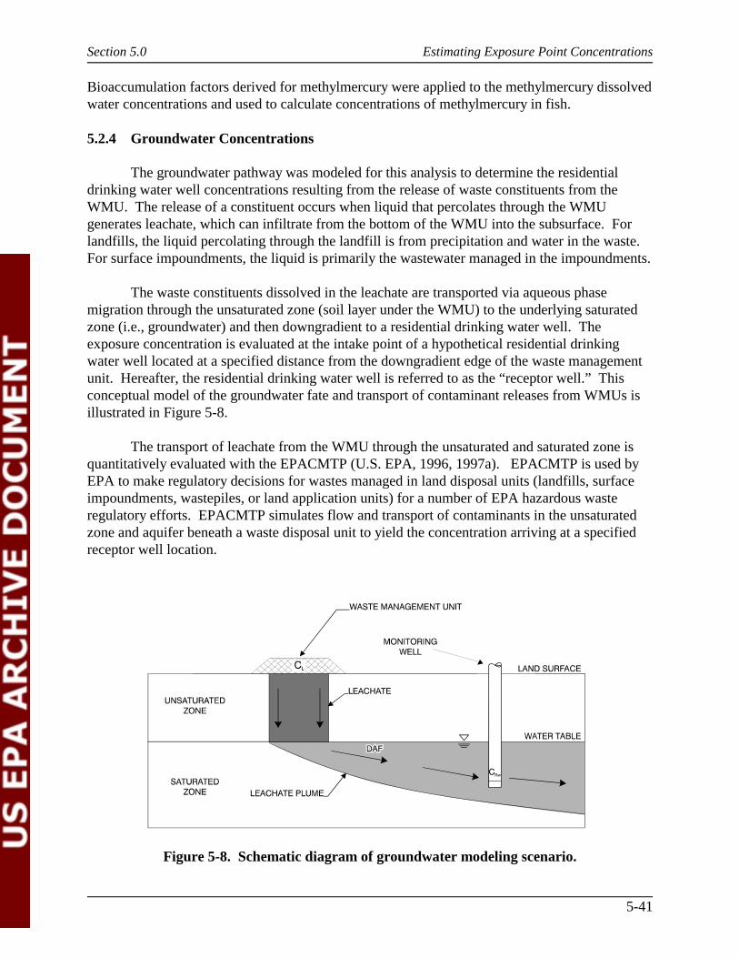
Section 5.0 Estimating Exposure Point Concentrations
5-41
Figure 5-8. Schematic diagram of groundwater modeling scenario.
Bioaccumulation factors derived for methylmercury were applied to the methylmercury dissolvedwater concentrations and used to calculate concentrations of methylmercury in fish.
5.2.4 Groundwater Concentrations
The groundwater pathway was modeled for this analysis to determine the residentialdrinking water well concentrations resulting from the release of waste constituents from theWMU. The release of a constituent occurs when liquid that percolates through the WMUgenerates leachate, which can infiltrate from the bottom of the WMU into the subsurface. Forlandfills, the liquid percolating through the landfill is from precipitation and water in the waste. For surface impoundments, the liquid is primarily the wastewater managed in the impoundments.
The waste constituents dissolved in the leachate are transported via aqueous phasemigration through the unsaturated zone (soil layer under the WMU) to the underlying saturatedzone (i.e., groundwater) and then downgradient to a residential drinking water well. Theexposure concentration is evaluated at the intake point of a hypothetical residential drinkingwater well located at a specified distance from the downgradient edge of the waste managementunit. Hereafter, the residential drinking water well is referred to as the “receptor well.” Thisconceptual model of the groundwater fate and transport of contaminant releases from WMUs isillustrated in Figure 5-8.
The transport of leachate from the WMU through the unsaturated and saturated zone is quantitatively evaluated with the EPACMTP (U.S. EPA, 1996, 1997a). EPACMTP is used byEPA to make regulatory decisions for wastes managed in land disposal units (landfills, surfaceimpoundments, wastepiles, or land application units) for a number of EPA hazardous wasteregulatory efforts. EPACMTP simulates flow and transport of contaminants in the unsaturatedzone and aquifer beneath a waste disposal unit to yield the concentration arriving at a specifiedreceptor well location.
Section 5.0 Estimating Exposure Point Concentrations
5-42
Fate and transport processes accounted for in the model are advection, hydrodynamicdispersion, equilibrium linear or nonlinear sorption, and transformation processes via chemicalhydrolysis. In this analysis, partition coefficients developed from data compiled from thescientific literature were used. More information on constituent-specific partition coefficients ispresented in Appendix H. The composite model consists of two coupled modules: (1) a one-dimensional module that simulates infiltration and dissolved contaminant transport through theunsaturated zone, and (2) a saturated zone flow and transport module. It is assumed that the soiland aquifer are uniform porous media and that flow and transport are described by Darcy’s lawand the advection-dispersion equation, respectively. EPACMTP does not account forpreferential pathways such as fractures and macropores or facilitated transport, which may affectmigration of strongly sorbing constituents such as metals.
The primary transport mechanisms in the subsurface are downward movement along withinfiltrating water flow in the unsaturated zone and movement along with ambient groundwaterflow in the saturated zone. The advective movement in the unsaturated zone is one-dimensional,while the saturated zone module accounts for three-dimensional flow and transport. The modelalso considers mixing due to hydrodynamic dispersion in both the unsaturated and saturatedzones. In the unsaturated zone, flow is gravity-driven and prevails in the vertically downwarddirection. Therefore, the flow is modeled in the unsaturated zone as one-dimensional in thevertical direction. It is also assumed that transverse dispersion (both mechanical dispersion andmolecular diffusion) is negligible in the unsaturated zone. This assumption is based on the factthat lateral migration due to transverse dispersion is negligible compared with the horizontaldimensions of the WMUs. In addition, this assumption is environmentally protective because itallows the leading front of the constituent plume to arrive at the water table with greater peakconcentration in the case of a finite source.
In the saturated zone, the movement of constituents is primarily driven by ambientgroundwater flow, which in turn is controlled by a regional hydraulic gradient and hydraulicconductivity in the aquifer formation. The model does take into account the effects of infiltrationfrom the waste source as well as regional recharge into the aquifer. The effect of infiltrationfrom the waste source is to increase the groundwater flow in the horizontal transverse andvertical directions underneath and in the immediate vicinity of the waste source as may resultfrom groundwater mounding. This three-dimensional flow pattern will enhance the horizontaland vertical spreading of the plume. The effect of regional recharge outside of the waste sourceis to cause a downward dip in the movement of the plume as it moves in the downgradientgroundwater flow direction.
In addition to advective movement along with groundwater flow, the model simulatesmixing of contaminants with groundwater due to hydrodynamic dispersion, which acts in thelongitudinal, i.e, along the groundwater flow direction, as well as in horizontal and verticaltransverse directions. The rate of movement of contaminants may be strongly affected bysorption reactions in both the unsaturated and saturated zone. The effect of sorption is expressedin a retardation factor, which is directly related to the magnitude of the constituent-specific Kd
value (Koc in the case of organics). Constituents with a zero or low Kd (or Koc) value will have aretardation factor of 1, or close to it, which indicates that they will move at the same velocity asthe groundwater, or close to it. Constituents with high Kd values, such as certain semivolatile
Section 5.0 Estimating Exposure Point Concentrations
5-43
R � 1 �b × Kd (5-1)
organic constituents and many metals, will have high retardation factors and may move manytimes slower than groundwater. The relationship between Kd and retardation factor is expressedas
where
R = retardation factor
b = soil or aquifer bulk density (mg)Kd = solid-water partition coefficient (g/cm3)
= water content (in unsaturated zone) or porosity (in saturated zone).
The concentration of constituents in both the unsaturated and saturated zone may befurther attenuated by biochemical transformation reactions. Although EPACMTP can, inprinciple, model a wide range of transformation processes as long as they can be represented as afirst-order process, in practice a more conservative approach is adopted in which onlydegradation of organic constituents via hydrolysis transformation processes is simulated. Forthose constituents that may be transformed via hydrolysis into toxic daughter products,EPACMTP can account for the formation and subsequent fate and transport of these daughterproducts. The COCs considered in this analysis are those identified in paint wastes and do notinclude degradation (or daughter) products. The effect of degradation products on chemicalconcentrations was evaluated in a screening analysis (Appendix T). Two sets of deterministicruns were conducted for surrogate chemicals consisting of parent-daughter products. Theconcentration of daughter product was evaluated at receptor wells and found to be negligible.
Hydrolysis rates were calculated from chemical-specific hydrolysis rate constants usingsoil and aquifer temperature and pH values. Whereas chemical hydrolysis can be accuratelymodeled as a function of these factors, many other types of transformation processes, such asbiodegradation, are much more site-specific and can be highly variable and therefore much moredifficult to simulate using a generic model such as EPACMTP. EPA is therefore using aconservative assumption that these processes do not occur; that is, biodegradation is notaccounted for. In the case of metals that may exist in multiple valence states, such as chromium(III) and chromium (VI), these species are modeled as separate constituents; no redoxtransformations are assumed to occur.
Whereas EPACMTP simulates steady-state flow in both the unsaturated zone and thesaturated zone; contaminant transport can be either steady-state or transient. Modeling flow assteady-state assumes that the infiltration and recharge, as well as ambient groundwater flowconditions, are representative of long-term average conditions that do not change over theduration of the simulation process. The model does not account for transient flow conditions thatmay result from temporal (e.g., seasonal) variations in precipitation and regional groundwaterflow. The EPACMTP model can accommodate either steady-state or transient contaminanttransport. Steady-state transport modeling corresponds to a very conservative risk scenario inwhich a waste unit continues to release contaminants indefinitely (continuous source), so that
Section 5.0 Estimating Exposure Point Concentrations
5-44
eventually the receptor well concentration reaches a constant, never changing value. In this analysis, transient transport simulations were performed. This analysis is referred to as a “finitesource” scenario because it explicitly takes into account the finite time period over which a wasteunit operates and releases contaminants, as well as the actual time it may take contaminants toreach the receptor well. The leachate concentrations calculated by the landfill partition modelwere used to calculate a total waste concentration to leachate concentration ratio, which was thenused to determine the length of time that the landfill will leach.
The output of EPACMTP is a prediction of the contaminant concentration arriving at adowngradient groundwater receptor well. This can be either a steady-state concentration value,corresponding to the continuous source scenario, or a time-dependent concentration,corresponding to the finite source scenario. In the latter case, the model can calculate either thepeak concentration arriving at the well or a maximum time-averaged concentration. In thisanalysis, a maximum 9-year average was used for all constituents. The 9-year exposure timeperiod corresponds to the average residence time used in the subsequent risk calculations. Themaximum 9-year average receptor well concentration represents the highest averageconcentration at the well over any 9-year time period.
The metals-modeling methodology in EPACMTP incorporates three options to specifythe Kd for a given metal:
� As a statistical distribution of values
� As an empirical distribution of values
� Chosen from adsorption isotherms coded into the EPACMTP program. Anisotherm is an expression of the equilibrium relationship between the aqueousconcentration and the sorbed concentration of a metal (or other constituent) atconstant temperature.
For this analysis, the Kd for most metals was defined as an empirical distribution when sufficientdata were available (i.e., nine or more data points based on a search of literature values). The Kd
for metals with fewer data available from the scientific literature was defined as a log uniformdistribution of values. The log uniform distribution was developed by taking the mean of thelogs of the available data and extending the distribution by 1.5 log units in both directions. Thethird option for determining the Kd involves the automated use of adsorption isotherms. Becausetechnical issues have been raised regarding the data supporting the adsorption isotherms, EPAdecided not to use this component of EPACMTP; thus, this third option was not used for any ofthe constituents in this analysis. More details about the development of statistical distributions ofKd values used in this analysis are presented in Appendix H.
Modeling of organic constituents was based on modeling four organic constituent groupsinstead of each individual organic constituent to reduce the number of model runs required. Fourorganic chemical groups were identified based on chemical properties of the constituents (i.e.,the organic carbon partition coefficient, Koc, and hydrolysis constant, Kh). The specificconstituents modeled as surrogates were ethylene glycol, chloroform, acrylonitrile, and
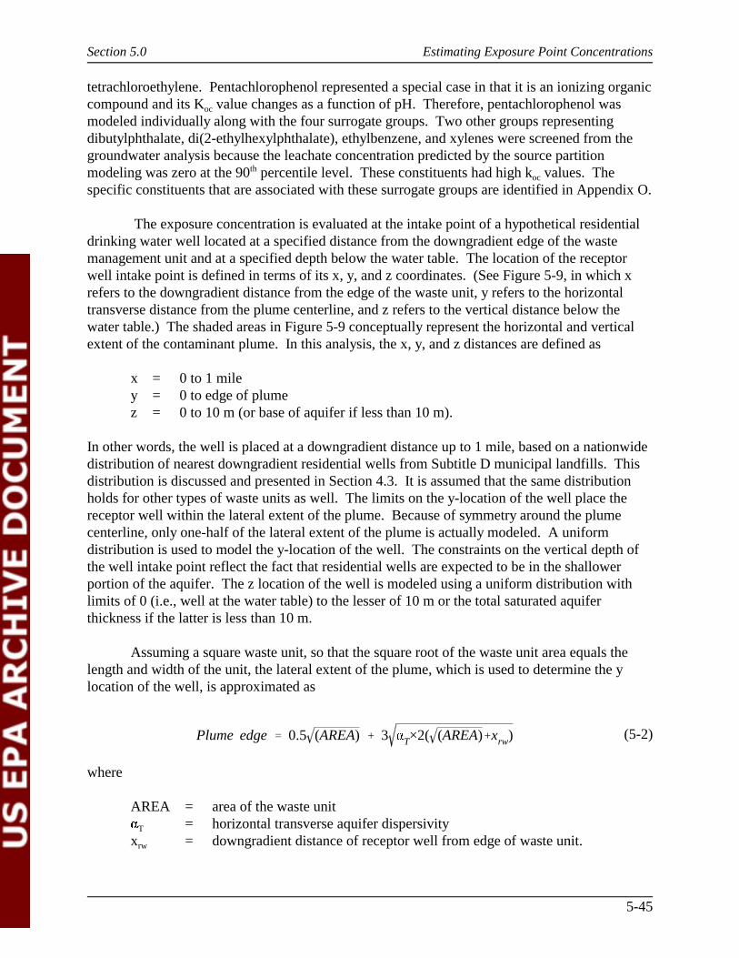
Section 5.0 Estimating Exposure Point Concentrations
5-45
Plume edge � 0.5 (AREA) � 3 T×2( (AREA)�xrw) (5-2)
tetrachloroethylene. Pentachlorophenol represented a special case in that it is an ionizing organiccompound and its Koc value changes as a function of pH. Therefore, pentachlorophenol wasmodeled individually along with the four surrogate groups. Two other groups representingdibutylphthalate, di(2-ethylhexylphthalate), ethylbenzene, and xylenes were screened from thegroundwater analysis because the leachate concentration predicted by the source partitionmodeling was zero at the 90th percentile level. These constituents had high koc values. Thespecific constituents that are associated with these surrogate groups are identified in Appendix O.
The exposure concentration is evaluated at the intake point of a hypothetical residentialdrinking water well located at a specified distance from the downgradient edge of the wastemanagement unit and at a specified depth below the water table. The location of the receptorwell intake point is defined in terms of its x, y, and z coordinates. (See Figure 5-9, in which xrefers to the downgradient distance from the edge of the waste unit, y refers to the horizontaltransverse distance from the plume centerline, and z refers to the vertical distance below thewater table.) The shaded areas in Figure 5-9 conceptually represent the horizontal and verticalextent of the contaminant plume. In this analysis, the x, y, and z distances are defined as
x = 0 to 1 miley = 0 to edge of plumez = 0 to 10 m (or base of aquifer if less than 10 m).
In other words, the well is placed at a downgradient distance up to 1 mile, based on a nationwidedistribution of nearest downgradient residential wells from Subtitle D municipal landfills. Thisdistribution is discussed and presented in Section 4.3. It is assumed that the same distributionholds for other types of waste units as well. The limits on the y-location of the well place thereceptor well within the lateral extent of the plume. Because of symmetry around the plumecenterline, only one-half of the lateral extent of the plume is actually modeled. A uniformdistribution is used to model the y-location of the well. The constraints on the vertical depth ofthe well intake point reflect the fact that residential wells are expected to be in the shallowerportion of the aquifer. The z location of the well is modeled using a uniform distribution withlimits of 0 (i.e., well at the water table) to the lesser of 10 m or the total saturated aquiferthickness if the latter is less than 10 m.
Assuming a square waste unit, so that the square root of the waste unit area equals thelength and width of the unit, the lateral extent of the plume, which is used to determine the ylocation of the well, is approximated as
where
AREA = area of the waste unit
T = horizontal transverse aquifer dispersivityxrw = downgradient distance of receptor well from edge of waste unit.
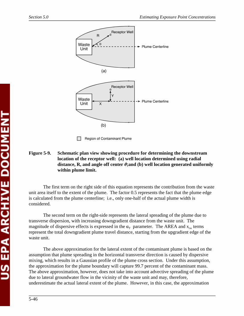
Section 5.0 Estimating Exposure Point Concentrations
5-46
Figure 5-9. Schematic plan view showing procedure for determining the downstreamlocation of the receptor well: (a) well location determined using radialdistance, R, and angle off center ;and (b) well location generated uniformlywithin plume limit.
The first term on the right side of this equation represents the contribution from the wasteunit area itself to the extent of the plume. The factor 0.5 represents the fact that the plume edgeis calculated from the plume centerline; i.e., only one-half of the actual plume width isconsidered.
The second term on the right-side represents the lateral spreading of the plume due totransverse dispersion, with increasing downgradient distance from the waste unit. Themagnitude of dispersive effects is expressed in the T parameter. The AREA and xrw termsrepresent the total downgradient plume travel distance, starting from the upgradient edge of thewaste unit.
The above approximation for the lateral extent of the contaminant plume is based on theassumption that plume spreading in the horizontal transverse direction is caused by dispersivemixing, which results in a Gaussian profile of the plume cross section. Under this assumption,the approximation for the plume boundary will capture 99.7 percent of the contaminant mass.The above approximation, however, does not take into account advective spreading of the plumedue to lateral groundwater flow in the vicinity of the waste unit and may, therefore,underestimate the actual lateral extent of the plume. However, in this case, the approximation
Section 5.0 Estimating Exposure Point Concentrations
5-47
will be conservative, as it will prevent placement of the well at the outer fringes of the plume,which will have the lowest concentrations compared to wells closer in.
Because the subsurface migration of some highly sorbing constituents (e.g., Cr III, Pb) may be very slow, it may take a long time for the plume to reach the receptor well, and the maximum 9-year exposure (see above) may not occur until a very long time after the waste unitceases operations. This time delay may be on the order of thousands of years. Appendix Upresents median and maximum time of arrival of peak concentration for constituents modeled inthis analysis. In this analysis, a maximum exposure time period of 10,000 years is used. In otherwords, if the model predicts that the maximum 9-year exposure has not yet occurred after 10,000years, the actual receptor well concentration at 10,000 years will be used in the risk calculations. Imposing this time limit discounts potential risks that may not occur until very far into the futurerelative to exposures and risks that are predicted to occur in the nearer term.
5.2.5 Predicting Indoor Air Concentrations
Constituents that have reached a residential groundwater well may be extracted and usedfor domestic purposes (e.g., showering). In this analysis, it is assumed that constituents thatreach a residential groundwater well will be used not only as drinking water, but also forshowering. This type of exposure is called indirect exposure because a constituent is passedfrom contaminated media to a receptor indirectly. The indirect exposure from showering occurswhen vapors are generated as a result of volatilization of the constituent in the domestic waterdrawn from the groundwater well.
Volatilization of constituents may occur with other indoor water uses as well. In previousanalyses, however, showering activity has been the dominant pathway for indoor air exposuresfor receptors using groundwater. Therefore, only showering activity is modeled in this analysis.
Exposure to constituents released into the indoor air from showering activity wasevaluated for the adult resident only. Young children are assumed to take baths primarily andthus not to encounter significant exposure to constituents released during showering activity. The adult resident is assumed to take one shower per day. The duration of each shower event isassumed to be a distribution of values ranging from 1 to 60 minutes. Exposure due to showeringwith contaminated residential groundwater is assumed to occur 350 days of the year, which isconsistent with exposure frequency assumptions made for other exposure pathways.
Appendix P presents the algorithms that are the basis of the shower model and theexposure factors used in the shower model.
5.3 Calculation of Food Chain Concentrations
Constituents can pass from contaminated air, soil, and surface water and reach people andwildlife through the food chain. For example, constituents that are transported in air may bedeposited on plants or onto soil in which the plants are growing. Constituents from the air andsoil may be accumulated in fruits and vegetables that are consumed by people. In addition, beefand dairy cattle may feed on forage, grain, and silage that is grown in contaminated areas. The

Section 5.0 Estimating Exposure Point Concentrations
5-48
beef and dairy products may be subsequently consumed by people. Similarly, constituents thatcontaminate surface water may be accumulated by fish, which are subsequently consumed by arecreational fisher.
This section presents the methodology used to calculate contaminant concentrations foreach of the food chain pathways considered. An approach was developed for a terrestrial foodchain to calculate concentrations of produce, beef, and milk that are consumed by the adult andchild farmer evaluated in this assessment. In addition, an approach was developed for an aquaticfood chain to calculate concentrations in fish that may be consumed by a recreational fisher.
5.3.1 Terrestrial Food Chain
The terrestrial food chain is designed to predict the accumulation of a contaminant in theedible parts of a plant from uptake of contaminants in soil and through translocation and directdeposition of contaminants in air. Concentrations are predicted for three main categories of foodcrops presumed to be eaten by humans: exposed fruits and vegetables, protected fruits, and rootvegetables. The terms “exposed” and “protected” refer to whether or not the edible portion of theproduce is exposed to the atmosphere. Examples include tomatoes (exposed vegetable), bananas(protected fruit), and potatoes (root vegetables).
In addition, the terrestrial food chain estimates the contaminant concentration in farmcrops for cattle. Vegetation consumed by cattle includes grain, forage, and silage. Grain isconsidered to be a protected vegetation and forage an exposed vegetation. Silage refers to anyplants harvested for animal consumption, whether protected or exposed. Silage is calculated asexposed vegetation; however, an empirical correction factor for silage takes into account thatsilage is partly protected and partly exposed.
Table 5-5 summarizes the mechanisms by which vegetation can be exposed tocontaminants. The three mechanisms are: deposition of particle-bound contaminants to exposedplant tissues, vapor-phase deposition of contaminants to exposed plant tissues, and root uptake. Exposed vegetation is subject to contamination via particulate deposition, vapor-phasedeposition, and root uptake, while protected vegetation is contaminated only through root uptakebecause the edible portion of the vegetation is not in direct contact with air. Accumulation byroot uptake can occur through the uptake of soil water for aboveground protected vegetables andfruit or by absorption into the outer parts of the root vegetables.
5.3.1.1 Aboveground Vegetation. Aboveground vegetation is subject to contaminationvia deposition of particle-bound contaminants, vapor transfer of contaminants, and root uptake asshown in Figure 5-10.
Deposition of Particle-Bound Contaminants. Particle-bound contaminants from the airare deposited by wet and dry deposition; thus they affect only exposed vegetation. As describedearlier, an air dispersion model was used to calculate the wet and dry deposition rates for theparticle-bound contaminants. The contaminants from dry deposition were assumed to remain onthe plant’s surface until weathering occurs. However, only a fraction of contaminant from wetdeposition remains on the plant’s surface; the rest washes off immediately.
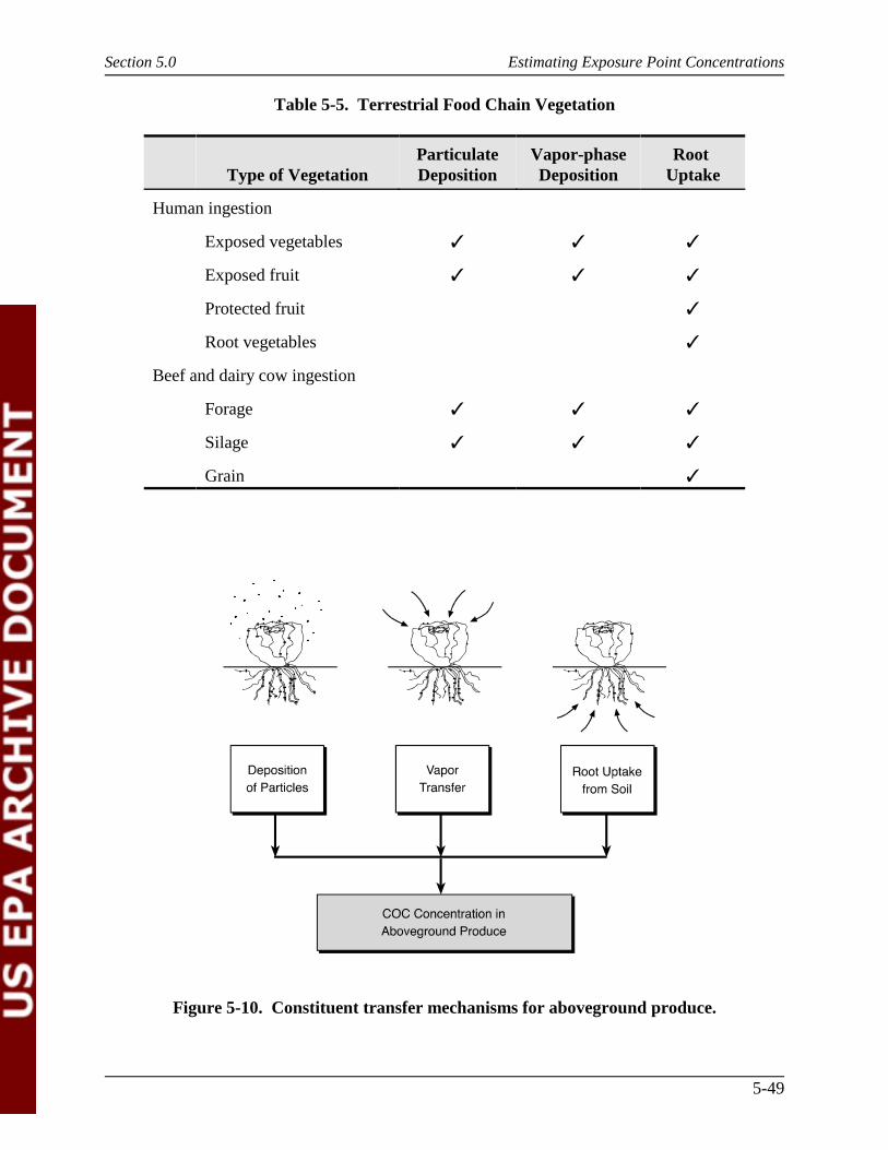
Section 5.0 Estimating Exposure Point Concentrations
5-49
Figure 5-10. Constituent transfer mechanisms for aboveground produce.
Table 5-5. Terrestrial Food Chain Vegetation
Type of VegetationParticulateDeposition
Vapor-phaseDeposition
Root Uptake
Human ingestion
Exposed vegetables � � �
Exposed fruit � � �
Protected fruit �
Root vegetables �
Beef and dairy cow ingestion
Forage � � �
Silage � � �
Grain �
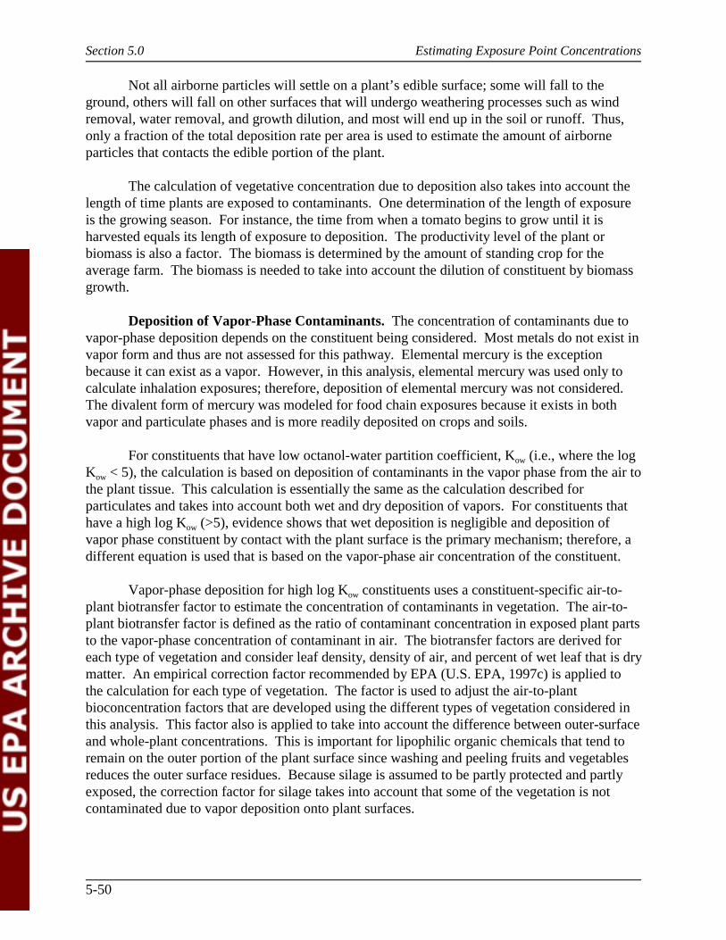
Section 5.0 Estimating Exposure Point Concentrations
5-50
Not all airborne particles will settle on a plant’s edible surface; some will fall to theground, others will fall on other surfaces that will undergo weathering processes such as wind removal, water removal, and growth dilution, and most will end up in the soil or runoff. Thus,only a fraction of the total deposition rate per area is used to estimate the amount of airborneparticles that contacts the edible portion of the plant.
The calculation of vegetative concentration due to deposition also takes into account thelength of time plants are exposed to contaminants. One determination of the length of exposureis the growing season. For instance, the time from when a tomato begins to grow until it isharvested equals its length of exposure to deposition. The productivity level of the plant orbiomass is also a factor. The biomass is determined by the amount of standing crop for theaverage farm. The biomass is needed to take into account the dilution of constituent by biomassgrowth.
Deposition of Vapor-Phase Contaminants. The concentration of contaminants due tovapor-phase deposition depends on the constituent being considered. Most metals do not exist invapor form and thus are not assessed for this pathway. Elemental mercury is the exceptionbecause it can exist as a vapor. However, in this analysis, elemental mercury was used only tocalculate inhalation exposures; therefore, deposition of elemental mercury was not considered. The divalent form of mercury was modeled for food chain exposures because it exists in bothvapor and particulate phases and is more readily deposited on crops and soils.
For constituents that have low octanol-water partition coefficient, Kow (i.e., where the logKow < 5), the calculation is based on deposition of contaminants in the vapor phase from the air tothe plant tissue. This calculation is essentially the same as the calculation described forparticulates and takes into account both wet and dry deposition of vapors. For constituents thathave a high log Kow (>5), evidence shows that wet deposition is negligible and deposition ofvapor phase constituent by contact with the plant surface is the primary mechanism; therefore, adifferent equation is used that is based on the vapor-phase air concentration of the constituent.
Vapor-phase deposition for high log Kow constituents uses a constituent-specific air-to-plant biotransfer factor to estimate the concentration of contaminants in vegetation. The air-to-plant biotransfer factor is defined as the ratio of contaminant concentration in exposed plant partsto the vapor-phase concentration of contaminant in air. The biotransfer factors are derived foreach type of vegetation and consider leaf density, density of air, and percent of wet leaf that is drymatter. An empirical correction factor recommended by EPA (U.S. EPA, 1997c) is applied tothe calculation for each type of vegetation. The factor is used to adjust the air-to-plantbioconcentration factors that are developed using the different types of vegetation considered inthis analysis. This factor also is applied to take into account the difference between outer-surfaceand whole-plant concentrations. This is important for lipophilic organic chemicals that tend toremain on the outer portion of the plant surface since washing and peeling fruits and vegetablesreduces the outer surface residues. Because silage is assumed to be partly protected and partlyexposed, the correction factor for silage takes into account that some of the vegetation is notcontaminated due to vapor deposition onto plant surfaces.

Section 5.0 Estimating Exposure Point Concentrations
5-51
Root Uptake. Plants take up contaminants in the soil through their roots bytranslocation. Water, which contains contaminants from the soil, moves up the roots, movingcontaminants to the aboveground shoots. Root uptake is a function of a constituent’s plant-soilbioconcentration factor. The plant-soil bioconcentration factor measures the constituent’s abilityto accumulate in plant tissue and is the ratio of constituent concentration in plants to theconcentration in soil.
For organics, an equation has been developed to calculate the plant-soil bioconcentrationfactor; for other constituents, this factor was developed based on measured data collected fromvarious sources. The plant-soil bioconcentration factor derived for organic constituents isdependent on the solubility of a constituent in water, which is inversely proportional to theoctanol-water partition coefficient, Kow. In constituents that are more lipophilic and do not movereadily through the roots, the bioconcentration factor is assumed to account for possibleresuspension and redeposition, which may add to constituent concentration.
5.3.1.2 Belowground Vegetation. In belowground plants, roots can take incontaminants from the soil that may accumulate in the edible portion of the plant. Thecalculation of concentrations in root vegetables varies depending on the constituent type. Formetals and mercury, the calculation is essentially the same as discussed for root uptake inaboveground plants. For organics, the calculation is a function of the root concentration factor,which is used to estimate the amount of constituent moving from the soil into the root vegetable.
Similar to the calculation for vapor-phase deposition, an empirical correction factor isapplied to the concentrations in belowground vegetables. The correction factor is applied toadjust the root concentration factor so that it is appropriate for bulky belowground root crops. The factor also accounts for constituent losses due to cleaning and cooking and the tendency oflipophilic contaminants to remain in the outer portions of the root (U.S. EPA, 1997c).
5.3.1.3 Animal Tissue Concentration. The animal products considered in this riskanalysis are beef and milk from beef and dairy cattle, respectively. The contaminantconcentrations in beef tissue and milk were estimated based on the amount of contaminant thecattle were assumed to have consumed through ingestion. Specifically, the ingestion rates forcattle were calculated for intake of plant material, incidental soil ingestion, and water ingestion. Plant ingestion comes from forage, grain, and silage. The animals are also assumed to ingestsoil, with which they come in contact during grazing or other activities on untilled soils. Astream located at the end of the agricultural field is used as the drinking water source for cattle. It is assumed that water is not treated prior to consumption by cattle. Therefore, calculations forthe ingestion of contaminants via drinking water for cattle are based on the total contaminantconcentration in the waterbody (i.e., dissolved and suspended sediment).
Different ingestion rates were used for beef and dairy cattle, depending on the amount offeed they consume and the activity patterns of the animals. For example, beef cattle are assumedto spend more time grazing and, therefore, have a higher incidental ingestion rate of soil. Theanimal concentrations also depend on biotransfer factors, which are the ratio of the contaminantconcentration in animal tissue to the daily intake of contaminant by the animal. Constituent-specific biotransfer factors were derived for both milk and beef. Chemical concentrations in
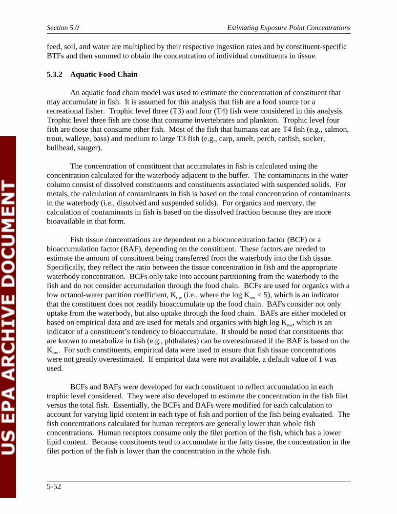
Section 5.0 Estimating Exposure Point Concentrations
5-52
feed, soil, and water are multiplied by their respective ingestion rates and by constituent-specificBTFs and then summed to obtain the concentration of individual constituents in tissue.
5.3.2 Aquatic Food Chain
An aquatic food chain model was used to estimate the concentration of constituent thatmay accumulate in fish. It is assumed for this analysis that fish are a food source for arecreational fisher. Trophic level three (T3) and four (T4) fish were considered in this analysis. Trophic level three fish are those that consume invertebrates and plankton. Trophic level fourfish are those that consume other fish. Most of the fish that humans eat are T4 fish (e.g., salmon,trout, walleye, bass) and medium to large T3 fish (e.g., carp, smelt, perch, catfish, sucker,bullhead, sauger).
The concentration of constituent that accumulates in fish is calculated using theconcentration calculated for the waterbody adjacent to the buffer. The contaminants in the watercolumn consist of dissolved constituents and constituents associated with suspended solids. Formetals, the calculation of contaminants in fish is based on the total concentration of contaminantsin the waterbody (i.e., dissolved and suspended solids). For organics and mercury, thecalculation of contaminants in fish is based on the dissolved fraction because they are morebioavailable in that form.
Fish tissue concentrations are dependent on a bioconcentration factor (BCF) or abioaccumulation factor (BAF), depending on the constituent. These factors are needed toestimate the amount of constituent being transferred from the waterbody into the fish tissue. Specifically, they reflect the ratio between the tissue concentration in fish and the appropriatewaterbody concentration. BCFs only take into account partitioning from the waterbody to thefish and do not consider accumulation through the food chain. BCFs are used for organics with alow octanol-water partition coefficient, Kow (i.e., where the log Kow < 5), which is an indicatorthat the constituent does not readily bioaccumulate up the food chain. BAFs consider not onlyuptake from the waterbody, but also uptake through the food chain. BAFs are either modeled orbased on empirical data and are used for metals and organics with high log Kow, which is anindicator of a constituent’s tendency to bioaccumulate. It should be noted that constituents thatare known to metabolize in fish (e.g., phthalates) can be overestimated if the BAF is based on theKow. For such constituents, empirical data were used to ensure that fish tissue concentrationswere not greatly overestimated. If empirical data were not available, a default value of 1 wasused.
BCFs and BAFs were developed for each constituent to reflect accumulation in eachtrophic level considered. They were also developed to estimate the concentration in the fish filetversus the total fish. Essentially, the BCFs and BAFs were modified for each calculation toaccount for varying lipid content in each type of fish and portion of the fish being evaluated. Thefish concentrations calculated for human receptors are generally lower than whole fishconcentrations. Human receptors consume only the filet portion of the fish, which has a lowerlipid content. Because constituents tend to accumulate in the fatty tissue, the concentration in thefilet portion of the fish is lower than the concentration in the whole fish.

Section 5.0 Estimating Exposure Point Concentrations
5-53
5.4. References
Atkinson, D., and R.F. Lee. 1992. Procedures for Substituting Values for Missing NWSMeteorological Data for Use in Regulatory Air Quality Models. U.S. EnvironmentalProtection Agency, Research Triangle Park, NC.
Cowherd, C., G.E. Muleski, P.J. Englehart, and D.A.Gillette. 1985. Rapid Assessment ofExposure to Particulate Emissions from Surface Contamination Sites. EPA/600/8-85/002. U.S. Environmental Protection Agency, Office of Research and Development,Office of Health and Environmental Assessment, Washington, DC. February.
Howard, P.H., R.S. Boethling, W.F. Jarvis, W.M. Meylan, and E.M. Michalenko, and Printup,H.T. (ed.) 1991. Handbook of Environmental Degradation Rates. Chelsea, MI: LewisPublishers, Inc.
Jury, W.A., W.F. Spencer, and W.J. Farmer. 1983. Behavior assessment model for traceorganics in soil: I. Model description. Journal of Environmental Quality 12(4):558-564.October.
Jury, W.A., D. Russo, G. Streile, and H. El Abd. 1990. Evolution of volatilization by organicchemicals residing below the soil surface. Water Resources Research 26(1):13-20.January.
Koester, C.J., and R.A. Hites. 1992. Wet and dry deposition of chlorinated dioxins and furans.Environmental Science and Technology 26:1375-1382.
NCDC, ERL, and NWS (National Climatic Data Center; Environmental Research Laboratories;National Weather Service). 1995. Cooperative Summary of the Day: TD3200-Period ofrecord through 1993 CD-ROM. Department of Commerce, National Oceanic andAtmospheric Administration, Asheville, NC. June.
NCDC (National Climatic Data Center and Forecast Systems Laboratory). 1997. RadiosondeData of North America, 1946-1996, Version 1.0, June 1997 (Updated).
PNNL (Pacific Northwest National Laboratory). 1999. Documentation for the FRAMES-HWIRTechnology Software System. Volume 1: System Overview. Prepared for the Office ofResearch and Development and Office of Solid Waste, U.S. Environmental ProtectionAgency, Washington, DC.
Shan, C., and D.B. Stephens. 1995. An analytical solution for vertical transport of volatilechemicals in the vadose zone. Journal of Contaminant Hydrology 18:259-277.
USDA (Department of Agriculture). 1971. Chapter 6: Sediment sources, yields, and deliveryratios. In: National Engineering Handbook, Section 3: Sedimentation, SoilConservation Service, Washington, DC. pp. 6-1 to 6-14.
Section 5.0 Estimating Exposure Point Concentrations
5-54
USDA (Department of Agriculture). 1978. Predicting Rainfall Erosion Losses: A Guide toConservation Planning. Agriculture Handbook No. 537. Science and EducationAdministration, Washington, DC.
U.S. DOC and U.S. DOE (U.S. Department of Commerce National Climatic Data Center andU.S. Department of Energy National Renewable Energy Laboratory). 1993. Solar andMeteorological Surface Observation Network (SAMSON) 1961-1990. Version 1.0.
U.S. EPA (Environmental Protection Agency). 1990. Methodology for Assessing Health RisksAssociated with Indirect Exposure to Combustor Emissions (Interim Final). EPA/600/6-90/003. Office of Health and Environmental Assessment, Washington, DC. January.
U.S. EPA (Environmental Protection Agency). 1993. Addendum to Methodology for AssessingHealth Risks Associated with Indirect Exposure to Combustor Emissions (ExternalReview Draft). EPA/600/AP-93/003. Exposure Assessment Group, Office of Health andEnvironmental Assessment, Washington, DC.
U.S. EPA (Environmental Protection Agency). 1994. 1:250,000 Scale Quadrangles ofLanduse/Landcover GIRAS Spatial Data in the Conterminous United States: Metadata. National GIS Program, Office of Information Resources Management, Washington, DC.Website at http://www.epa.gov/ngispgm3/nsdi/projects/giras.htm
U.S. EPA (Environmental Protection Agency). 1995a. Compilation of Air Pollutant EmissionFactors, Volume 1: Stationary Point and Area Sources. 5th Edition. AP-42. PB95-196028INZ. Office of Air Quality Planning and Standards, Research Triangle Park, NC.
U.S. EPA (Environmental Protection Agency). 1995b. Draft User’s Guide for the IndustrialSource Complex (ISC3) Dispersion Models. Volume I: User Instructions (Revised).EPA-454/B-95-003a. Emissions, Monitoring, and Analysis Division, Office of AirQuality Planning and Standards, Research Triangle Park, NC.
U.S. EPA (Environmental Protection Agency). 1995c. PCRAMMET User’s Guide (Draft). Office of Air Quality Planning and Standards, Research Triangle Park, NC.
U.S. EPA (Environmental Protection Agency). 1995d. User’s Guide for the Industrial SourceComplex (ISC3) Dispersion Models. Volume II: Description of Model Algorithms. EPA-454/B-95-003b. Emissions, Monitoring, and Analysis Division, Office of AirQuality Planning and Standards, Research Triangle Park, NC.
US EPA (Environmental Protection Agency). 1996. EPACMTP: Background Document.Office of Solid Waste, Washington, DC 20460.
U.S. EPA (Environmental Protection Agency). 1997a. EPACMTP: User’s Guide. Office ofSolid Waste, Washington, DC 20460.
Section 5.0 Estimating Exposure Point Concentrations
5-55
U.S. EPA (Environmental Protection Agency). 1997b. Mercury Study Report to Congress. Volume III, Fate and Transport of Mercury in the Environment. EPA 452/R-97/005. Office of Air Quality Planning and Standards and Office of Research and Development,Washington, DC.
U.S. EPA (Environmental Protection Agency). 1997c. The Parameter Guidance Document. ACompanion Document to the Methodology for Assessing Health Risks Associated withMultiple Pathways Exposure to Combustion Emissions. (Internal draft) NCEA-2038. National Center for Environmental Assessment, Cincinnati, OH.
U.S. EPA (Environmental Protection Agency). 1998a. Human Health Risk Assessment Protocolfor Hazardous Waste Combustion Facilities, Volume One. EPA-530-D-98-001A. Officeof Solid Waste and Emergency Response, Washington, DC.
U.S. EPA (Environmental Protection Agency). 1998b. Methodology for Assessing Health RisksAssociated with Multiple Pathways of Exposure to Combustor Emissions. Update toMethodology for Assessing Health Risks Associated with Indirect Exposure to CombustorEmissions. EPA-600/R-98/137. National Center for Environmental Assessment,Cincinnati, OH.
U.S. EPA (Environmental Protection Agency). 1999a. Addendum. User’s Guide for theIndustrial Source Complex (ISC3) Dispersion Models. Volume I: User Instructions forthe Revised ISCST3 Model (Dated 99155). Office of Air Quality Planning and Standards,Research Triangle Park, NC.
U.S. EPA (Environmental Protection Agency). 1999b. Source Modules for NonwastewaterWaste Management Units (Land Application Units, Waste Piles, and Landfills):Background and Implementation for the Multimedia, Multipathway, and MultireceptorRisk Assessment (3MRA) for HWIR99. Office of Solid Waste, Washington, DC. October.
U.S. EPA (Environmental Protection Agency). 1999c. Appendix W to Part 51--Guideline onAir Quality Models. Code of Federal Regulations 40 CFR 51.
USN, USAF, and U.S. DOC (U.S. Navy; U.S. Air Force; U.S. Department of Commerce). 1992.International Station Meteorological Climate Summary (ISMCS). Version 2.0. Availableon CD-ROM from the National Climatic Data Center, Asheville, NC. June.
van der Leeden, F., F.L. Troise, and D.K. Todd. 1990. The Water Encyclopedia. 2nd edition. Chelsea, Michigan: Lewis Publishers. p. 176.

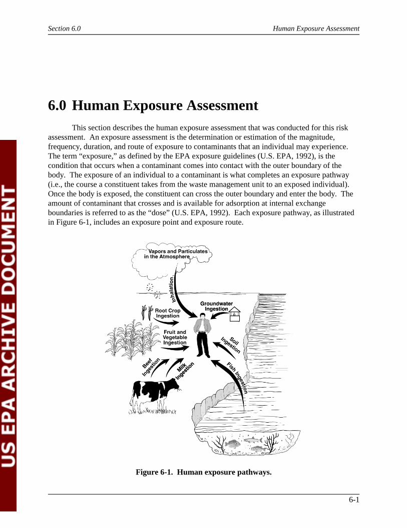
Section 6.0 Human Exposure Assessment
6-1
Figure 6-1. Human exposure pathways.
6.0 Human Exposure AssessmentThis section describes the human exposure assessment that was conducted for this risk
assessment. An exposure assessment is the determination or estimation of the magnitude,frequency, duration, and route of exposure to contaminants that an individual may experience. The term “exposure,” as defined by the EPA exposure guidelines (U.S. EPA, 1992), is thecondition that occurs when a contaminant comes into contact with the outer boundary of thebody. The exposure of an individual to a contaminant is what completes an exposure pathway(i.e., the course a constituent takes from the waste management unit to an exposed individual). Once the body is exposed, the constituent can cross the outer boundary and enter the body. Theamount of contaminant that crosses and is available for adsorption at internal exchangeboundaries is referred to as the “dose” (U.S. EPA, 1992). Each exposure pathway, as illustratedin Figure 6-1, includes an exposure point and exposure route.
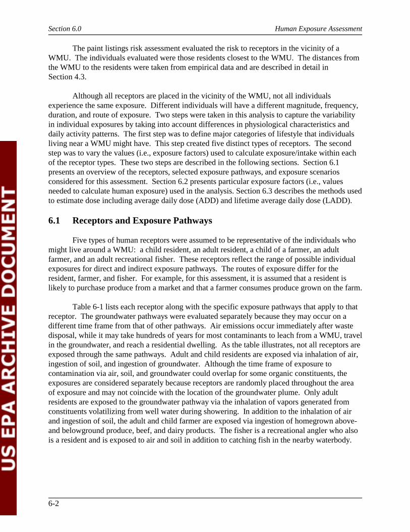
Section 6.0 Human Exposure Assessment
6-2
The paint listings risk assessment evaluated the risk to receptors in the vicinity of aWMU. The individuals evaluated were those residents closest to the WMU. The distances fromthe WMU to the residents were taken from empirical data and are described in detail inSection 4.3.
Although all receptors are placed in the vicinity of the WMU, not all individualsexperience the same exposure. Different individuals will have a different magnitude, frequency,duration, and route of exposure. Two steps were taken in this analysis to capture the variabilityin individual exposures by taking into account differences in physiological characteristics anddaily activity patterns. The first step was to define major categories of lifestyle that individualsliving near a WMU might have. This step created five distinct types of receptors. The secondstep was to vary the values (i.e., exposure factors) used to calculate exposure/intake within eachof the receptor types. These two steps are described in the following sections. Section 6.1presents an overview of the receptors, selected exposure pathways, and exposure scenariosconsidered for this assessment. Section 6.2 presents particular exposure factors (i.e., valuesneeded to calculate human exposure) used in the analysis. Section 6.3 describes the methods usedto estimate dose including average daily dose (ADD) and lifetime average daily dose (LADD).
6.1 Receptors and Exposure Pathways
Five types of human receptors were assumed to be representative of the individuals whomight live around a WMU: a child resident, an adult resident, a child of a farmer, an adultfarmer, and an adult recreational fisher. These receptors reflect the range of possible individualexposures for direct and indirect exposure pathways. The routes of exposure differ for theresident, farmer, and fisher. For example, for this assessment, it is assumed that a resident islikely to purchase produce from a market and that a farmer consumes produce grown on the farm.
Table 6-1 lists each receptor along with the specific exposure pathways that apply to thatreceptor. The groundwater pathways were evaluated separately because they may occur on adifferent time frame from that of other pathways. Air emissions occur immediately after wastedisposal, while it may take hundreds of years for most contaminants to leach from a WMU, travelin the groundwater, and reach a residential dwelling. As the table illustrates, not all receptors areexposed through the same pathways. Adult and child residents are exposed via inhalation of air,ingestion of soil, and ingestion of groundwater. Although the time frame of exposure tocontamination via air, soil, and groundwater could overlap for some organic constituents, theexposures are considered separately because receptors are randomly placed throughout the areaof exposure and may not coincide with the location of the groundwater plume. Only adultresidents are exposed to the groundwater pathway via the inhalation of vapors generated fromconstituents volatilizing from well water during showering. In addition to the inhalation of airand ingestion of soil, the adult and child farmer are exposed via ingestion of homegrown above-and belowground produce, beef, and dairy products. The fisher is a recreational angler who alsois a resident and is exposed to air and soil in addition to catching fish in the nearby waterbody.
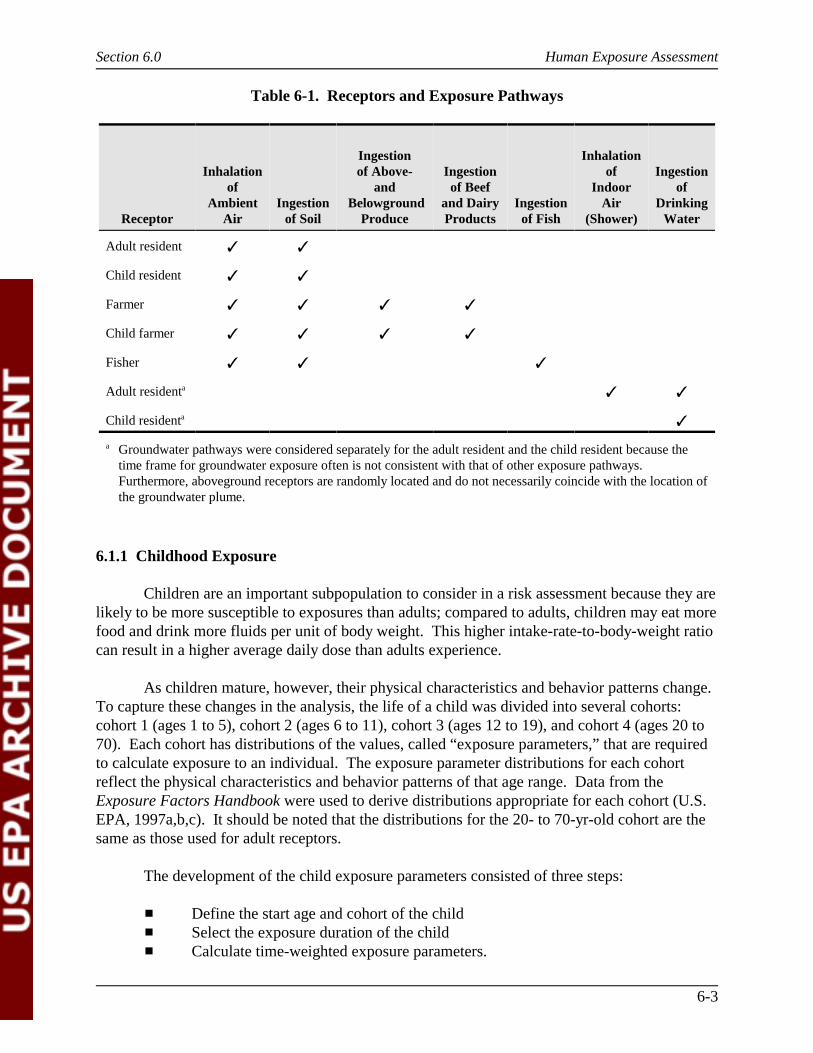
Section 6.0 Human Exposure Assessment
6-3
Table 6-1. Receptors and Exposure Pathways
Receptor
Inhalationof
AmbientAir
Ingestionof Soil
Ingestionof Above-
and Belowground
Produce
Ingestionof Beef
and DairyProducts
Ingestionof Fish
Inhalationof
IndoorAir
(Shower)
Ingestionof
DrinkingWater
Adult resident � �
Child resident � �
Farmer � � � �
Child farmer � � � �
Fisher � � �
Adult residenta � �
Child residenta �
a Groundwater pathways were considered separately for the adult resident and the child resident because thetime frame for groundwater exposure often is not consistent with that of other exposure pathways. Furthermore, aboveground receptors are randomly located and do not necessarily coincide with the location ofthe groundwater plume.
6.1.1 Childhood Exposure
Children are an important subpopulation to consider in a risk assessment because they arelikely to be more susceptible to exposures than adults; compared to adults, children may eat morefood and drink more fluids per unit of body weight. This higher intake-rate-to-body-weight ratiocan result in a higher average daily dose than adults experience.
As children mature, however, their physical characteristics and behavior patterns change. To capture these changes in the analysis, the life of a child was divided into several cohorts:cohort 1 (ages 1 to 5), cohort 2 (ages 6 to 11), cohort 3 (ages 12 to 19), and cohort 4 (ages 20 to70). Each cohort has distributions of the values, called “exposure parameters,” that are requiredto calculate exposure to an individual. The exposure parameter distributions for each cohortreflect the physical characteristics and behavior patterns of that age range. Data from theExposure Factors Handbook were used to derive distributions appropriate for each cohort (U.S.EPA, 1997a,b,c). It should be noted that the distributions for the 20- to 70-yr-old cohort are thesame as those used for adult receptors.
The development of the child exposure parameters consisted of three steps:
� Define the start age and cohort of the child� Select the exposure duration of the child� Calculate time-weighted exposure parameters.
Section 6.0 Human Exposure Assessment
6-4
EPTW �(EP1 × ED1) � (EP2 × ED2) � (EP3 × ED3) � (EP4 × ED4)
ED(6-1)
To capture the higher intake-rate-to-body-weight ratio of children, a start age between the ages of1 and 6 was selected. For the probabilistic analysis, a start age between these ages was selectedrandomly for each iteration. For the deterministic analysis, the start age was set at 3 years.
To select the exposure duration for each of the 10,000 iterations in the probabilisticanalysis, a distribution was chosen to define the exposure duration based on the start age. Forexample, if the start age was 2, the distribution for cohort 1, a 1- to 5-yr-old, was used to defineexposure duration. However, if the start age was 6, the distribution developed for cohort 2,children between ages 6 and 11, was used to define exposure duration. In the deterministicapproach, a central tendency or high-end exposure duration was used for each cohort rather thana distribution.
After the start age and the exposure duration were defined for a given iteration, all theother exposure parameters needed to calculate exposure to a child were randomly selected fromthe distributions associated with each of the cohorts through which the child would age. Oncethis selection was finished, an exposure parameter selected from each cohort was time-weightedand combined with its corresponding value from the other cohorts to create a single time-weighted parameter. For example, the beef ingestion rates selected from each age cohort weretime-weighted according to the number of years the child remained in the cohort and combinedto generate a single time-adjusted beef ingestion rate for the child. The same was done for all theparameters (e.g., body weight, inhalation rate, fruit ingestion rate) required to perform anassessment of exposure. The equation used to combine each cohort’s exposure parameters intoone time-weighted exposure parameter is as follows:
where
EPTW = time-weighted exposure parameter (e.g., ingestion rate of milk, body weight)EP1 = exposure parameter cohort 1 (ages 1 to 5)ED1 = time spent in cohort 1EP2 = exposure parameter cohort 2 (ages 6 to 11)ED2 = time spent in cohort 2EP3 = exposure parameter cohort 3 (ages 12 to 19)ED3 = time spent in cohort 3EP4 = exposure parameter cohort 4 (ages 20 to 70)ED4 = time spent in cohort 4ED = total exposure duration of the receptor (sum of ED1 + ED2 +ED3 + ED4).
The time-weighted exposure parameters were used to assess the carcinogenic risk to thechild receptors. Because noncarcinogenic risk is generally higher for lower age groups due tohigher intake rates relative to body weight, the assessment of noncancer hazards to children usedthe exposure parameters from the cohort corresponding to the child’s start age.
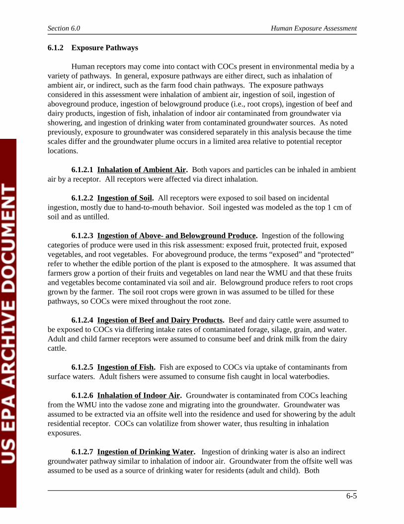
Section 6.0 Human Exposure Assessment
6-5
6.1.2 Exposure Pathways
Human receptors may come into contact with COCs present in environmental media by avariety of pathways. In general, exposure pathways are either direct, such as inhalation ofambient air, or indirect, such as the farm food chain pathways. The exposure pathwaysconsidered in this assessment were inhalation of ambient air, ingestion of soil, ingestion ofaboveground produce, ingestion of belowground produce (i.e., root crops), ingestion of beef anddairy products, ingestion of fish, inhalation of indoor air contaminated from groundwater viashowering, and ingestion of drinking water from contaminated groundwater sources. As notedpreviously, exposure to groundwater was considered separately in this analysis because the timescales differ and the groundwater plume occurs in a limited area relative to potential receptorlocations.
6.1.2.1 Inhalation of Ambient Air. Both vapors and particles can be inhaled in ambientair by a receptor. All receptors were affected via direct inhalation.
6.1.2.2 Ingestion of Soil. All receptors were exposed to soil based on incidentalingestion, mostly due to hand-to-mouth behavior. Soil ingested was modeled as the top 1 cm ofsoil and as untilled.
6.1.2.3 Ingestion of Above- and Belowground Produce. Ingestion of the followingcategories of produce were used in this risk assessment: exposed fruit, protected fruit, exposedvegetables, and root vegetables. For aboveground produce, the terms “exposed” and “protected”refer to whether the edible portion of the plant is exposed to the atmosphere. It was assumed thatfarmers grow a portion of their fruits and vegetables on land near the WMU and that these fruitsand vegetables become contaminated via soil and air. Belowground produce refers to root cropsgrown by the farmer. The soil root crops were grown in was assumed to be tilled for thesepathways, so COCs were mixed throughout the root zone.
6.1.2.4 Ingestion of Beef and Dairy Products. Beef and dairy cattle were assumed tobe exposed to COCs via differing intake rates of contaminated forage, silage, grain, and water. Adult and child farmer receptors were assumed to consume beef and drink milk from the dairycattle.
6.1.2.5 Ingestion of Fish. Fish are exposed to COCs via uptake of contaminants fromsurface waters. Adult fishers were assumed to consume fish caught in local waterbodies.
6.1.2.6 Inhalation of Indoor Air. Groundwater is contaminated from COCs leachingfrom the WMU into the vadose zone and migrating into the groundwater. Groundwater wasassumed to be extracted via an offsite well into the residence and used for showering by the adultresidential receptor. COCs can volatilize from shower water, thus resulting in inhalationexposures.
6.1.2.7 Ingestion of Drinking Water. Ingestion of drinking water is also an indirectgroundwater pathway similar to inhalation of indoor air. Groundwater from the offsite well wasassumed to be used as a source of drinking water for residents (adult and child). Both
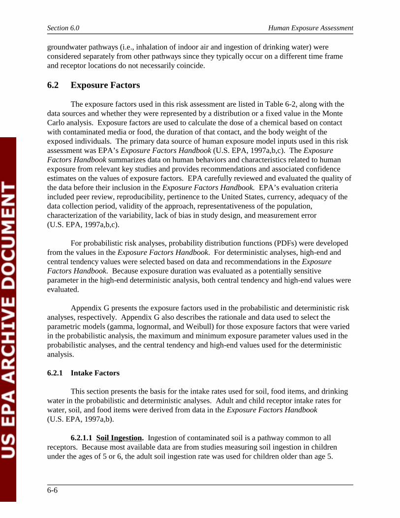
Section 6.0 Human Exposure Assessment
6-6
groundwater pathways (i.e., inhalation of indoor air and ingestion of drinking water) wereconsidered separately from other pathways since they typically occur on a different time frameand receptor locations do not necessarily coincide.
6.2 Exposure Factors
The exposure factors used in this risk assessment are listed in Table 6-2, along with thedata sources and whether they were represented by a distribution or a fixed value in the MonteCarlo analysis. Exposure factors are used to calculate the dose of a chemical based on contactwith contaminated media or food, the duration of that contact, and the body weight of theexposed individuals. The primary data source of human exposure model inputs used in this riskassessment was EPA’s Exposure Factors Handbook (U.S. EPA, 1997a,b,c). The ExposureFactors Handbook summarizes data on human behaviors and characteristics related to humanexposure from relevant key studies and provides recommendations and associated confidenceestimates on the values of exposure factors. EPA carefully reviewed and evaluated the quality ofthe data before their inclusion in the Exposure Factors Handbook. EPA’s evaluation criteriaincluded peer review, reproducibility, pertinence to the United States, currency, adequacy of thedata collection period, validity of the approach, representativeness of the population,characterization of the variability, lack of bias in study design, and measurement error(U.S. EPA, 1997a,b,c).
For probabilistic risk analyses, probability distribution functions (PDFs) were developedfrom the values in the Exposure Factors Handbook. For deterministic analyses, high-end andcentral tendency values were selected based on data and recommendations in the ExposureFactors Handbook. Because exposure duration was evaluated as a potentially sensitiveparameter in the high-end deterministic analysis, both central tendency and high-end values wereevaluated.
Appendix G presents the exposure factors used in the probabilistic and deterministic riskanalyses, respectively. Appendix G also describes the rationale and data used to select theparametric models (gamma, lognormal, and Weibull) for those exposure factors that were variedin the probabilistic analysis, the maximum and minimum exposure parameter values used in theprobabilistic analyses, and the central tendency and high-end values used for the deterministicanalysis.
6.2.1 Intake Factors
This section presents the basis for the intake rates used for soil, food items, and drinkingwater in the probabilistic and deterministic analyses. Adult and child receptor intake rates forwater, soil, and food items were derived from data in the Exposure Factors Handbook(U.S. EPA, 1997a,b).
6.2.1.1 Soil Ingestion. Ingestion of contaminated soil is a pathway common to allreceptors. Because most available data are from studies measuring soil ingestion in childrenunder the ages of 5 or 6, the adult soil ingestion rate was used for children older than age 5.
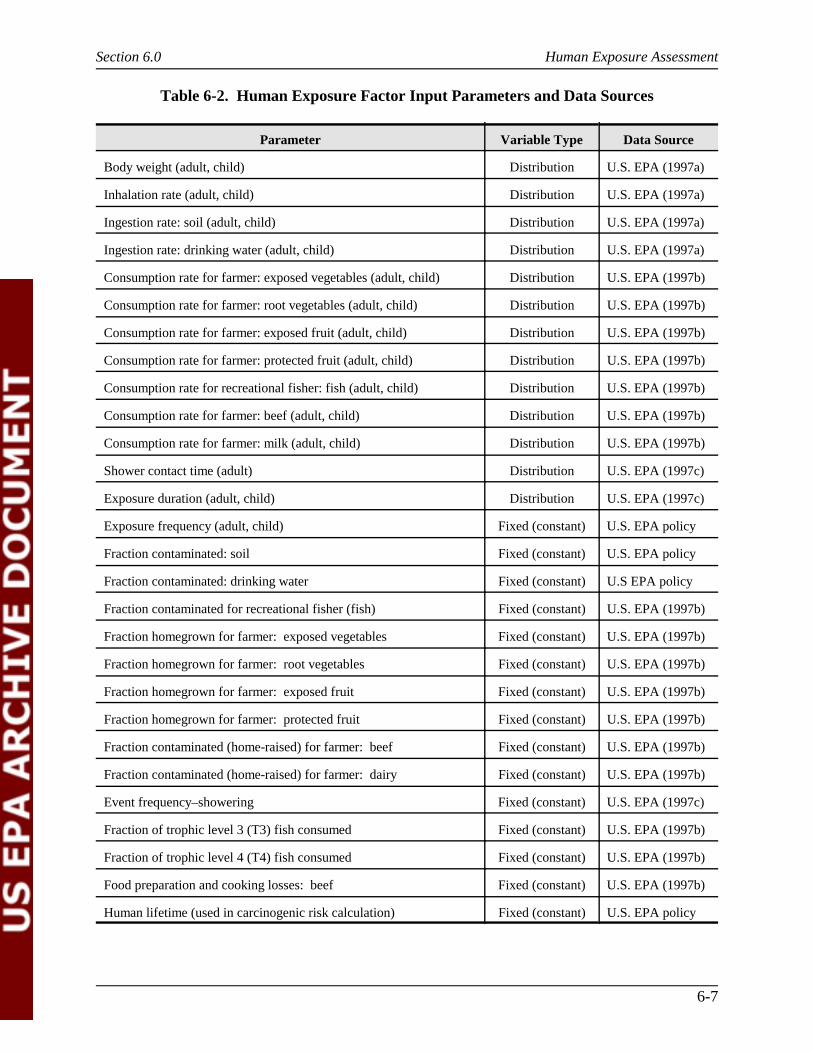
Section 6.0 Human Exposure Assessment
6-7
Table 6-2. Human Exposure Factor Input Parameters and Data Sources
Parameter Variable Type Data Source
Body weight (adult, child) Distribution U.S. EPA (1997a)
Inhalation rate (adult, child) Distribution U.S. EPA (1997a)
Ingestion rate: soil (adult, child) Distribution U.S. EPA (1997a)
Ingestion rate: drinking water (adult, child) Distribution U.S. EPA (1997a)
Consumption rate for farmer: exposed vegetables (adult, child) Distribution U.S. EPA (1997b)
Consumption rate for farmer: root vegetables (adult, child) Distribution U.S. EPA (1997b)
Consumption rate for farmer: exposed fruit (adult, child) Distribution U.S. EPA (1997b)
Consumption rate for farmer: protected fruit (adult, child) Distribution U.S. EPA (1997b)
Consumption rate for recreational fisher: fish (adult, child) Distribution U.S. EPA (1997b)
Consumption rate for farmer: beef (adult, child) Distribution U.S. EPA (1997b)
Consumption rate for farmer: milk (adult, child) Distribution U.S. EPA (1997b)
Shower contact time (adult) Distribution U.S. EPA (1997c)
Exposure duration (adult, child) Distribution U.S. EPA (1997c)
Exposure frequency (adult, child) Fixed (constant) U.S. EPA policy
Fraction contaminated: soil Fixed (constant) U.S. EPA policy
Fraction contaminated: drinking water Fixed (constant) U.S EPA policy
Fraction contaminated for recreational fisher (fish) Fixed (constant) U.S. EPA (1997b)
Fraction homegrown for farmer: exposed vegetables Fixed (constant) U.S. EPA (1997b)
Fraction homegrown for farmer: root vegetables Fixed (constant) U.S. EPA (1997b)
Fraction homegrown for farmer: exposed fruit Fixed (constant) U.S. EPA (1997b)
Fraction homegrown for farmer: protected fruit Fixed (constant) U.S. EPA (1997b)
Fraction contaminated (home-raised) for farmer: beef Fixed (constant) U.S. EPA (1997b)
Fraction contaminated (home-raised) for farmer: dairy Fixed (constant) U.S. EPA (1997b)
Event frequency–showering Fixed (constant) U.S. EPA (1997c)
Fraction of trophic level 3 (T3) fish consumed Fixed (constant) U.S. EPA (1997b)
Fraction of trophic level 4 (T4) fish consumed Fixed (constant) U.S. EPA (1997b)
Food preparation and cooking losses: beef Fixed (constant) U.S. EPA (1997b)
Human lifetime (used in carcinogenic risk calculation) Fixed (constant) U.S. EPA policy
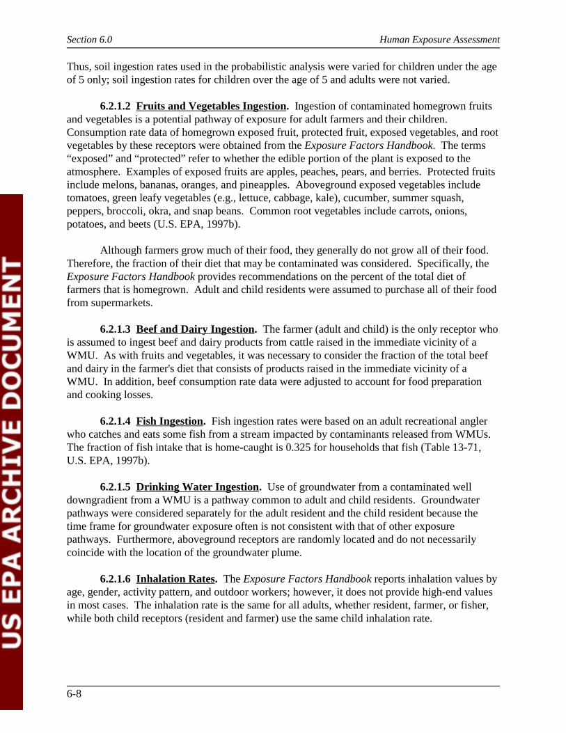
Section 6.0 Human Exposure Assessment
6-8
Thus, soil ingestion rates used in the probabilistic analysis were varied for children under the ageof 5 only; soil ingestion rates for children over the age of 5 and adults were not varied.
6.2.1.2 Fruits and Vegetables Ingestion. Ingestion of contaminated homegrown fruitsand vegetables is a potential pathway of exposure for adult farmers and their children. Consumption rate data of homegrown exposed fruit, protected fruit, exposed vegetables, and rootvegetables by these receptors were obtained from the Exposure Factors Handbook. The terms“exposed” and “protected” refer to whether the edible portion of the plant is exposed to theatmosphere. Examples of exposed fruits are apples, peaches, pears, and berries. Protected fruitsinclude melons, bananas, oranges, and pineapples. Aboveground exposed vegetables includetomatoes, green leafy vegetables (e.g., lettuce, cabbage, kale), cucumber, summer squash,peppers, broccoli, okra, and snap beans. Common root vegetables include carrots, onions,potatoes, and beets (U.S. EPA, 1997b).
Although farmers grow much of their food, they generally do not grow all of their food. Therefore, the fraction of their diet that may be contaminated was considered. Specifically, theExposure Factors Handbook provides recommendations on the percent of the total diet offarmers that is homegrown. Adult and child residents were assumed to purchase all of their foodfrom supermarkets.
6.2.1.3 Beef and Dairy Ingestion. The farmer (adult and child) is the only receptor whois assumed to ingest beef and dairy products from cattle raised in the immediate vicinity of aWMU. As with fruits and vegetables, it was necessary to consider the fraction of the total beefand dairy in the farmer's diet that consists of products raised in the immediate vicinity of aWMU. In addition, beef consumption rate data were adjusted to account for food preparationand cooking losses.
6.2.1.4 Fish Ingestion. Fish ingestion rates were based on an adult recreational anglerwho catches and eats some fish from a stream impacted by contaminants released from WMUs. The fraction of fish intake that is home-caught is 0.325 for households that fish (Table 13-71,U.S. EPA, 1997b).
6.2.1.5 Drinking Water Ingestion. Use of groundwater from a contaminated welldowngradient from a WMU is a pathway common to adult and child residents. Groundwaterpathways were considered separately for the adult resident and the child resident because thetime frame for groundwater exposure often is not consistent with that of other exposurepathways. Furthermore, aboveground receptors are randomly located and do not necessarilycoincide with the location of the groundwater plume.
6.2.1.6 Inhalation Rates. The Exposure Factors Handbook reports inhalation values byage, gender, activity pattern, and outdoor workers; however, it does not provide high-end valuesin most cases. The inhalation rate is the same for all adults, whether resident, farmer, or fisher,while both child receptors (resident and farmer) use the same child inhalation rate.
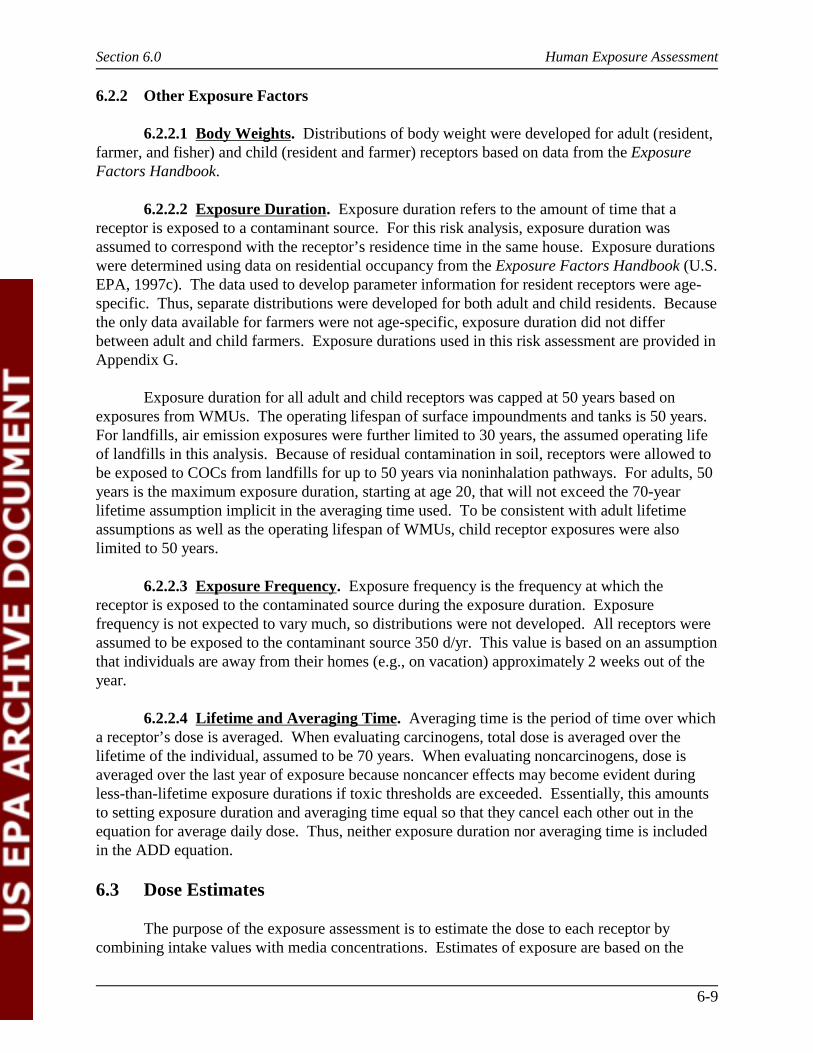
Section 6.0 Human Exposure Assessment
6-9
6.2.2 Other Exposure Factors
6.2.2.1 Body Weights. Distributions of body weight were developed for adult (resident,farmer, and fisher) and child (resident and farmer) receptors based on data from the ExposureFactors Handbook.
6.2.2.2 Exposure Duration. Exposure duration refers to the amount of time that areceptor is exposed to a contaminant source. For this risk analysis, exposure duration wasassumed to correspond with the receptor’s residence time in the same house. Exposure durationswere determined using data on residential occupancy from the Exposure Factors Handbook (U.S.EPA, 1997c). The data used to develop parameter information for resident receptors were age-specific. Thus, separate distributions were developed for both adult and child residents. Becausethe only data available for farmers were not age-specific, exposure duration did not differbetween adult and child farmers. Exposure durations used in this risk assessment are provided inAppendix G.
Exposure duration for all adult and child receptors was capped at 50 years based onexposures from WMUs. The operating lifespan of surface impoundments and tanks is 50 years. For landfills, air emission exposures were further limited to 30 years, the assumed operating lifeof landfills in this analysis. Because of residual contamination in soil, receptors were allowed tobe exposed to COCs from landfills for up to 50 years via noninhalation pathways. For adults, 50years is the maximum exposure duration, starting at age 20, that will not exceed the 70-yearlifetime assumption implicit in the averaging time used. To be consistent with adult lifetimeassumptions as well as the operating lifespan of WMUs, child receptor exposures were alsolimited to 50 years.
6.2.2.3 Exposure Frequency. Exposure frequency is the frequency at which thereceptor is exposed to the contaminated source during the exposure duration. Exposurefrequency is not expected to vary much, so distributions were not developed. All receptors wereassumed to be exposed to the contaminant source 350 d/yr. This value is based on an assumptionthat individuals are away from their homes (e.g., on vacation) approximately 2 weeks out of theyear.
6.2.2.4 Lifetime and Averaging Time. Averaging time is the period of time over whicha receptor’s dose is averaged. When evaluating carcinogens, total dose is averaged over thelifetime of the individual, assumed to be 70 years. When evaluating noncarcinogens, dose isaveraged over the last year of exposure because noncancer effects may become evident duringless-than-lifetime exposure durations if toxic thresholds are exceeded. Essentially, this amountsto setting exposure duration and averaging time equal so that they cancel each other out in theequation for average daily dose. Thus, neither exposure duration nor averaging time is includedin the ADD equation.
6.3 Dose Estimates
The purpose of the exposure assessment is to estimate the dose to each receptor bycombining intake values with media concentrations. Estimates of exposure are based on the
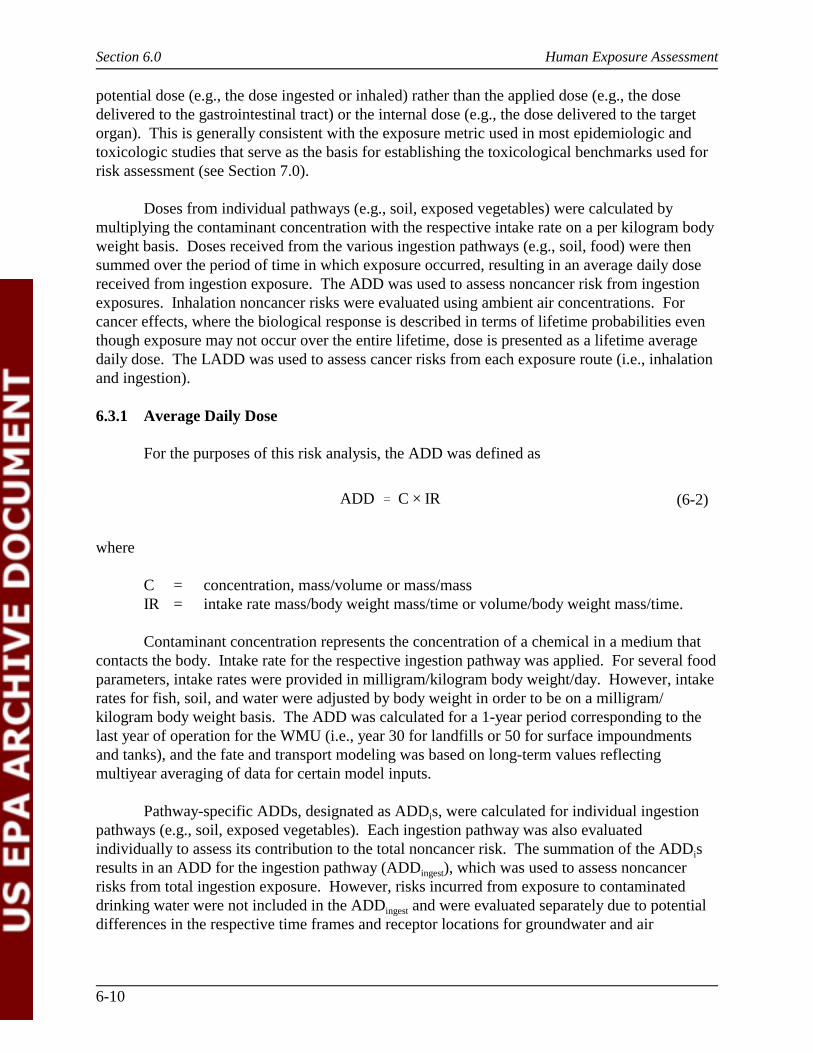
Section 6.0 Human Exposure Assessment
6-10
ADD � C × IR (6-2)
potential dose (e.g., the dose ingested or inhaled) rather than the applied dose (e.g., the dosedelivered to the gastrointestinal tract) or the internal dose (e.g., the dose delivered to the targetorgan). This is generally consistent with the exposure metric used in most epidemiologic andtoxicologic studies that serve as the basis for establishing the toxicological benchmarks used forrisk assessment (see Section 7.0).
Doses from individual pathways (e.g., soil, exposed vegetables) were calculated bymultiplying the contaminant concentration with the respective intake rate on a per kilogram bodyweight basis. Doses received from the various ingestion pathways (e.g., soil, food) were thensummed over the period of time in which exposure occurred, resulting in an average daily dosereceived from ingestion exposure. The ADD was used to assess noncancer risk from ingestionexposures. Inhalation noncancer risks were evaluated using ambient air concentrations. Forcancer effects, where the biological response is described in terms of lifetime probabilities eventhough exposure may not occur over the entire lifetime, dose is presented as a lifetime averagedaily dose. The LADD was used to assess cancer risks from each exposure route (i.e., inhalationand ingestion).
6.3.1 Average Daily Dose
For the purposes of this risk analysis, the ADD was defined as
where
C = concentration, mass/volume or mass/massIR = intake rate mass/body weight mass/time or volume/body weight mass/time.
Contaminant concentration represents the concentration of a chemical in a medium thatcontacts the body. Intake rate for the respective ingestion pathway was applied. For several foodparameters, intake rates were provided in milligram/kilogram body weight/day. However, intakerates for fish, soil, and water were adjusted by body weight in order to be on a milligram/kilogram body weight basis. The ADD was calculated for a 1-year period corresponding to thelast year of operation for the WMU (i.e., year 30 for landfills or 50 for surface impoundmentsand tanks), and the fate and transport modeling was based on long-term values reflectingmultiyear averaging of data for certain model inputs.
Pathway-specific ADDs, designated as ADDis, were calculated for individual ingestionpathways (e.g., soil, exposed vegetables). Each ingestion pathway was also evaluatedindividually to assess its contribution to the total noncancer risk. The summation of the ADDisresults in an ADD for the ingestion pathway (ADDingest), which was used to assess noncancerrisks from total ingestion exposure. However, risks incurred from exposure to contaminateddrinking water were not included in the ADDingest and were evaluated separately due to potentialdifferences in the respective time frames and receptor locations for groundwater and air
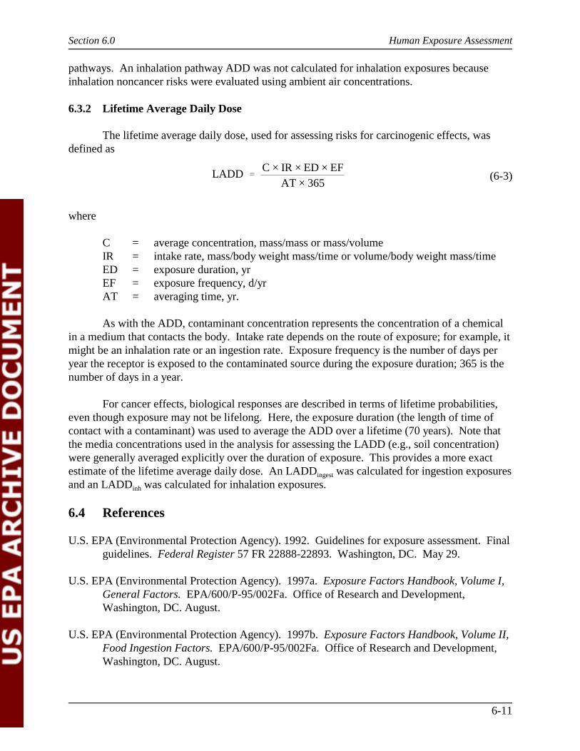
Section 6.0 Human Exposure Assessment
6-11
LADD �C × IR × ED × EF
AT × 365(6-3)
pathways. An inhalation pathway ADD was not calculated for inhalation exposures becauseinhalation noncancer risks were evaluated using ambient air concentrations.
6.3.2 Lifetime Average Daily Dose
The lifetime average daily dose, used for assessing risks for carcinogenic effects, wasdefined as
where
C = average concentration, mass/mass or mass/volumeIR = intake rate, mass/body weight mass/time or volume/body weight mass/timeED = exposure duration, yrEF = exposure frequency, d/yrAT = averaging time, yr.
As with the ADD, contaminant concentration represents the concentration of a chemicalin a medium that contacts the body. Intake rate depends on the route of exposure; for example, itmight be an inhalation rate or an ingestion rate. Exposure frequency is the number of days peryear the receptor is exposed to the contaminated source during the exposure duration; 365 is thenumber of days in a year.
For cancer effects, biological responses are described in terms of lifetime probabilities,even though exposure may not be lifelong. Here, the exposure duration (the length of time ofcontact with a contaminant) was used to average the ADD over a lifetime (70 years). Note thatthe media concentrations used in the analysis for assessing the LADD (e.g., soil concentration)were generally averaged explicitly over the duration of exposure. This provides a more exactestimate of the lifetime average daily dose. An LADDingest was calculated for ingestion exposuresand an LADDinh was calculated for inhalation exposures.
6.4 References
U.S. EPA (Environmental Protection Agency). 1992. Guidelines for exposure assessment. Finalguidelines. Federal Register 57 FR 22888-22893. Washington, DC. May 29.
U.S. EPA (Environmental Protection Agency). 1997a. Exposure Factors Handbook, Volume I,General Factors. EPA/600/P-95/002Fa. Office of Research and Development,Washington, DC. August.
U.S. EPA (Environmental Protection Agency). 1997b. Exposure Factors Handbook, Volume II,Food Ingestion Factors. EPA/600/P-95/002Fa. Office of Research and Development,Washington, DC. August.

Section 6.0 Human Exposure Assessment
6-12
U.S. EPA (Environmental Protection Agency). 1997c. Exposure Factors Handbook, Volume III,Activity Factors. EPA/600/P-95/002Fa. Office of Research and Development,Washington, DC. August.


![Assessment of benzo[a]pyrene concentrations in the United ...4.1.2 Point source modelling 11 4.1.3 Meteorological data 11 5 Prediction of BAP concentrations in 2003 and 2010, 2015](https://img.pdfslide.net/doc/110x75/61192bd4788b5e3eb47c51a2/assessment-of-benzoapyrene-concentrations-in-the-united-412-point-source.jpg)