04/18/23 1

Evaluation of Probability Evaluation of Probability ForecastsForecasts

Shulamith T GrossShulamith T Gross

CCity ity UUniversity of niversity of NNew ew YYork ork

BBaruch aruch CCollege ollege

Joint work with Joint work with

Tze Leung Lai, David Bo Shen: Tze Leung Lai, David Bo Shen: SStanford tanford UUniversity niversity

Catherine Huber Catherine Huber UUniversitee niversitee RRene ene DDescartesescartes

Rutgers 4.30.2012Rutgers 4.30.2012

04/18/23 2

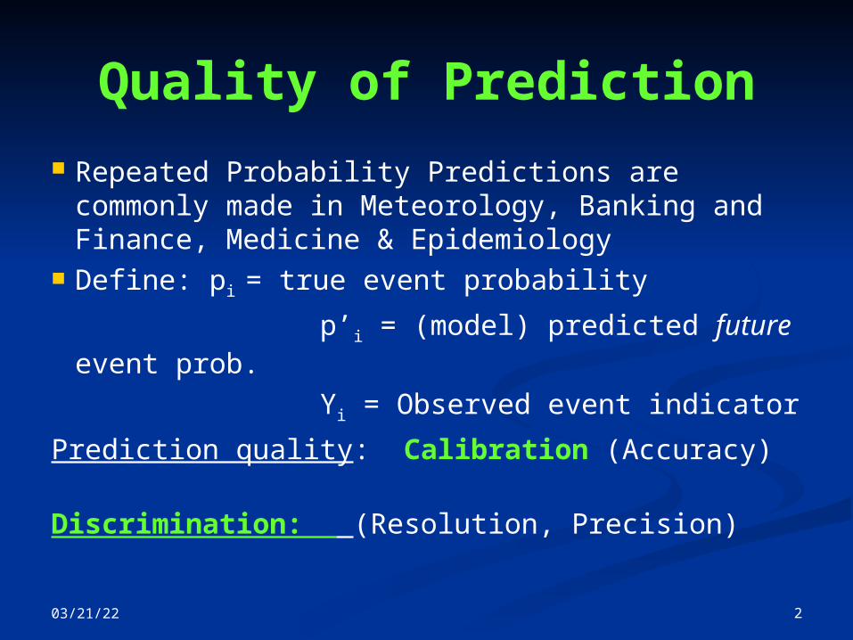
Quality of Prediction

Repeated Probability Predictions are commonly made in Meteorology, Banking and Finance, Medicine & Epidemiology

Define: pi = true event probability

p’i = (model) predicted future event prob.

Yi = Observed event indicator

Prediction quality: Calibration (Accuracy) Discrimination: (Resolution, Precision)

04/18/23 3

OUTLINEOUTLINE Evaluation of probability forecasts in

meteorology & Banking (Accuracy) Scores (Brier, Good), proper scores,

Winkler’s skill scores (w loss or utility)

L’L’nn = n = n-1 -1 Σ Σ 11≤i≤n≤i≤n (Y (Yi i – p’– p’ii))22

Reliability diagrams: Bin data according to predicted risk p’p’ii and plot the observed relative frequency of events in each bin center.

04/18/23 4

OUTLINE 2: Measures of OUTLINE 2: Measures of Predictiveness of modelsPredictiveness of models

MedicineMedicine: Scores are increasingly used. : Scores are increasingly used. EpidemiologyEpidemiology: Curves: ROC, Predictiveness: Curves: ROC, Predictiveness

Plethora of indices of Plethora of indices of reliability/discriminationreliability/discrimination: : AUC = P[p’AUC = P[p’1 1 > p’> p’22| Y| Y11=1, Y=1, Y22=0] =0] (Concordance. (Concordance.

One predictor)One predictor) Net Reclassification Index.Net Reclassification Index.

NRI = P[p’’>p’|Y=1]-P[p’’>p’|Y=0]- NRI = P[p’’>p’|Y=1]-P[p’’>p’|Y=0]-

{P[p’’<p’|Y=1]-P[p’’<p’|Y=0]} {P[p’’<p’|Y=1]-P[p’’<p’|Y=0]} Improved Discrimination IndexImproved Discrimination Index (“sign” (“sign”“-”)“-”)

IDI= E[p’’-p’|Y=1] - E[p’’-p’|Y=0] IDI= E[p’’-p’|Y=1] - E[p’’-p’|Y=0] (two predictors)(two predictors) RR22 = 1 – = 1 – ΣΣ(Y(Yii-p’-p’ii))22//ΣΣ (Y (Yii-Ybar)-Ybar)22 R-sq differencesR-sq differences

04/18/23 5

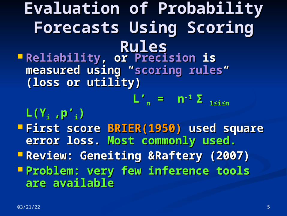
Evaluation of Probability Evaluation of Probability Forecasts Using Scoring Forecasts Using Scoring

RulesRules ReliabilityReliability, or, or Precision Precision is is

measured using “measured using “scoring rulesscoring rules“ “ (loss or utility)(loss or utility)

L’L’nn = n = n-1 -1 Σ Σ 11≤i≤n≤i≤n L(Y L(Yi i ,p’,p’ii)) First score First score BRIER(1950) BRIER(1950) used used

square error loss. square error loss. Most commonly Most commonly used.used.

Review: Geneiting &Raftery (2007)Review: Geneiting &Raftery (2007) Problem: very few inference tools Problem: very few inference tools

are availableare available

04/18/23 6

Earlier Contributions Proper scores (using loss functions) EEpp[L(Y,p)] ≤ E[L(Y,p)] ≤ Epp[L(Y,p’)][L(Y,p’)] InferenceInference: Tests of : Tests of HH00: p: pii = p’ = p’ii all all i=1,…,ni=1,…,n Cox(1958) in model Cox(1958) in model logit(plogit(pii)= )=

11++22logit(p’logit(p’ii)) Too restrictive. Need to estimate the true Too restrictive. Need to estimate the true

score-not test for perfect prediction.score-not test for perfect prediction. Related workRelated work: Econometrics. Evaluation of : Econometrics. Evaluation of

linear models. linear models. Emphasis on predicting YEmphasis on predicting Y. . Giacomini and White (Econometrica 2006)Giacomini and White (Econometrica 2006)

04/18/23 7

Statistical ConsiderationsStatistical Considerations

L’L’nn = n = n-1 -1 Σ Σ 11≤i≤n≤i≤n L(Y L(Yi i ,p’,p’ii) ) attempts to attempts to estimateestimate

LLnn = n = n-1 -1 Σ Σ 11≤i≤n≤i≤n L(p L(pi i ,p’,p’ii)) ‘population ‘population parameter’parameter’

Squared error loss Squared error loss L(p,p’) = (p – p’)L(p,p’) = (p – p’)22

Kullback-Leibler divergence (Good, 1952):Kullback-Leibler divergence (Good, 1952): L(p,p’) = p log(p/p’) + (1-p) log( L(p,p’) = p log(p/p’) + (1-p) log(

(1-p)/(1-p’))(1-p)/(1-p’)) How good is L’ in estimating L?How good is L’ in estimating L?

04/18/23 8

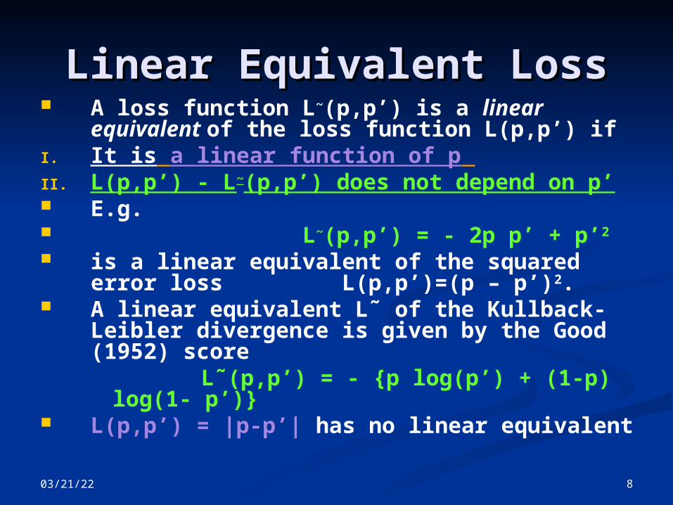
Linear Equivalent LossLinear Equivalent Loss A loss function L~(p,p’) is a linear

equivalent of the loss function L(p,p’) if I. It is a linear function of p II. L(p,p’) - L~(p,p’) does not depend on p’ E.g. L~(p,p’) = - 2p p’ + p’2

is a linear equivalent of the squared error loss L(p,p’)=(p – p’)2.

A linear equivalent L˜ of the Kullback-Leibler divergence is given by the Good (1952) score

L˜(p,p’) = - {p log(p’) + (1-p) log(1- p’)}

L(p,p’) = |p-p’| has no linear equivalent

04/18/23 9

LINEAR EQUIVALENTS-2LINEAR EQUIVALENTS-2 We allow all forecast p’k to depend on an

information set Fk-1 consisting of all event, forecast histories, and other covariates before Yk is observed, as well as the true p1…pk. The conditional distribution of Yi given Fi-1 is Bernoulli(pi), with

P(Yi = 1|Fi-1) = pi Dawid (1982, 1993) Martingale use in testing

hyp context Suppose L(p; p’) is linear in p, as in the case of

linear equivalents of general loss functions. Then

E[ L(Yi, p’i )| Fi-1] = L(pi,p’i) so L(Yi,p’i) - L(pi,p’i) is a martingale difference

sequence with respect to {Fi-1}.

04/18/23 10

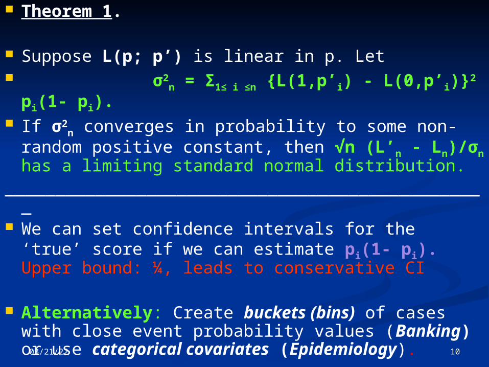
Theorem 1.

Suppose L(p; p’) is linear in p. Let σ2

n = Σ1≤ i ≤n {L(1,p’i) - L(0,p’i)}2 pi(1- pi).

If σ2n converges in probability to some non-

random positive constant, then √n (L’n - Ln)/σn has a limiting standard normal distribution.

________________________________________________ We can set confidence intervals for the ‘true’

score if we can estimate pi(1- pi). Upper bound: ¼, leads to conservative CI

Alternatively: Create buckets (bins) of cases with close event probability values (Banking) or use categorical covariates (Epidemiology).

04/18/23 11

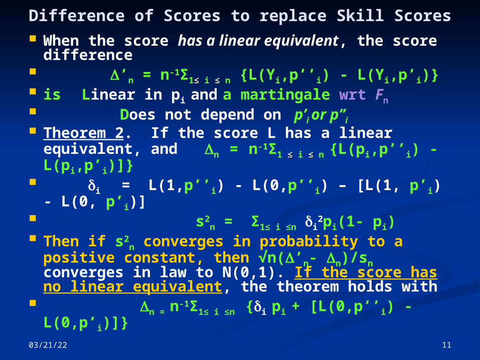
Difference of Scores to replace Skill Scores When the score has a linear equivalent, the

score difference ’n = n-1Σ1≤ ≤ i ≤≤ n {L(Yi,p’’i) - L(Yi,p’i)} is Linear in pi and a martingale wrt Fn Does not depend on p’i or p’’i Theorem 2. If the score L has a linear

equivalent, and n = n-1Σ1 ≤≤ i ≤≤ n {L(pi,p’’i) - L(pi,p’i)]}

i = L(1,p’’i) - L(0,p’’i) – [L(1, p’i) - L(0, p’i)]

s2n = Σ1≤ i ≤n i

2pi(1- pi) Then if s2

n converges in probability to a positive constant, then √n(’n- n)/sn converges in law to N(0,1). If the score has no linear equivalent, the theorem holds with

n = n-1Σ1≤ i ≤n {i pi + [L(0,p’’i) - L(0,p’i)]}

04/18/23 12

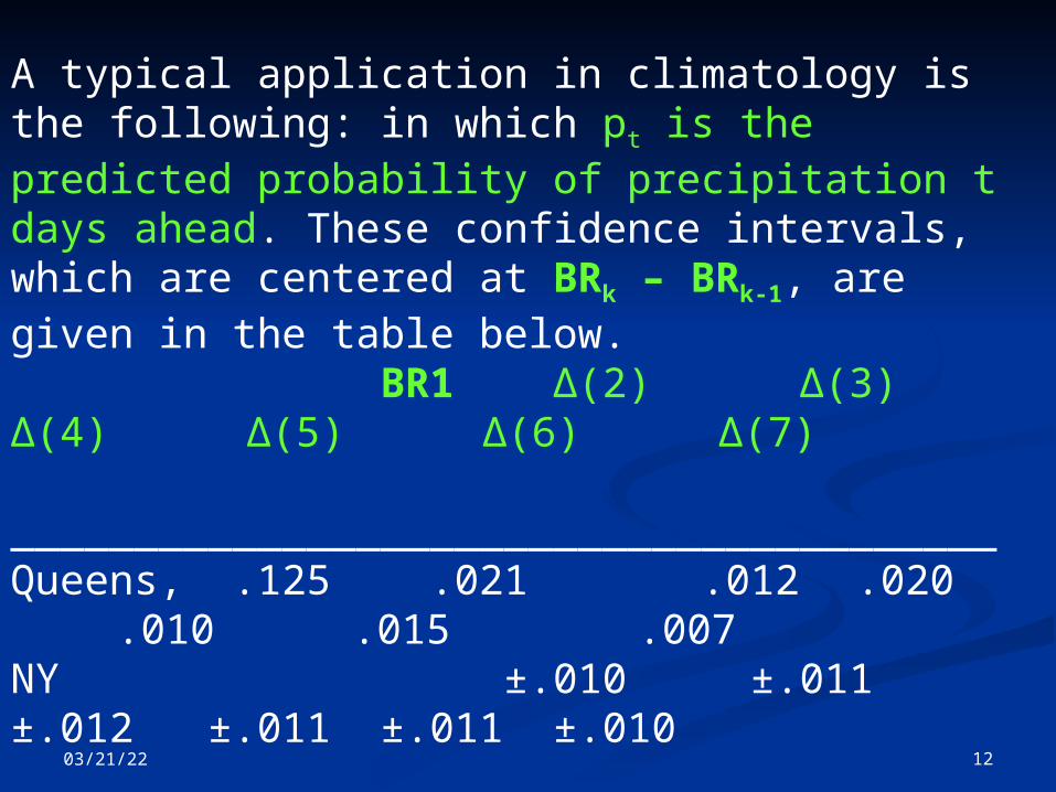
A typical application in climatology is the following: in which pt is the predicted probability of precipitation t days ahead. These confidence intervals, which are centered at BRk – BRk-1, are given in the table below. BR1 Δ(2) Δ(3) Δ(4) Δ(5) Δ(6) Δ(7) ________________________________________Queens, .125 .021 .012 .020 .010 .015

.007NY ±.010 ±.011 ±.012 ±.011 ±.011 ±.010

Jefferson .159 .005 .005 .007 .024 .000 .008

City, MO ±.010 ± .011 ±.011 ±.010 ±.010 ±.008

Brier scores B1 and Conservative 95% confidence intervals for Δ(k).

04/18/23 13

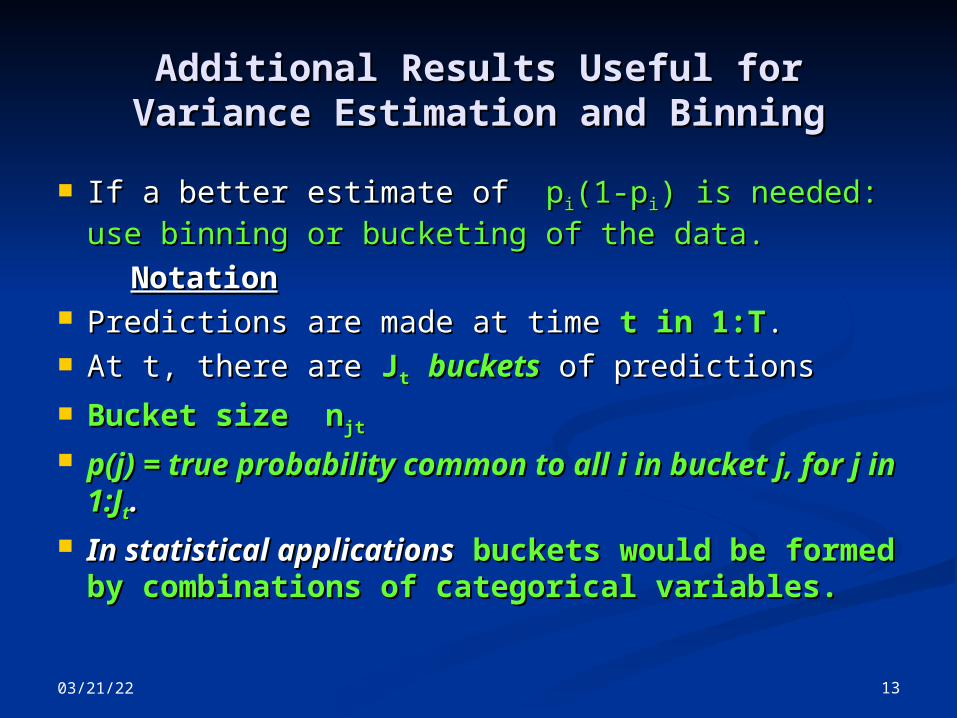
Additional Results Useful for Variance Additional Results Useful for Variance Estimation and BinningEstimation and Binning

If a better estimate of If a better estimate of ppii(1-p(1-pii) is needed: use ) is needed: use binning or bucketing of the data. binning or bucketing of the data.

NotationNotation Predictions are made at time Predictions are made at time t in 1:Tt in 1:T. . At t, there are At t, there are JJtt bucketsbuckets of predictions of predictions

Bucket size nBucket size njtjt p(j) = true probability common to all i in p(j) = true probability common to all i in

bucket j, for j in 1:Jbucket j, for j in 1:Jtt..

In statistical applicationsIn statistical applications buckets would be buckets would be formed by combinations of categorical formed by combinations of categorical variables.variables.

04/18/23 14

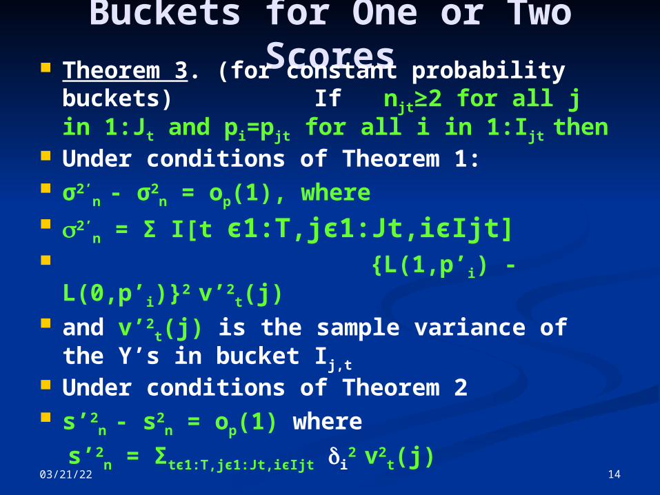
Buckets for One or Two Scores Theorem 3. (for constant probability

buckets) If njt≥2 for all j in 1:Jt and pi=pjt for all i in 1:Ijt then

Under conditions of Theorem 1: σ2’

n - σ2n = op(1), where

2’n = Σ I[t є1:T,jє1:Jt,iєIjt]

{L(1,p’i) - L(0,p’i)}2 v’2t(j)

and v’2t(j) is the sample variance of

the Y’s in bucket Ij,t

Under conditions of Theorem 2 s’2

n - s2n = op(1) where

s’2n = Σtє1:T,jє1:Jt,iєIjt i

2 v2t(j)

04/18/23 15

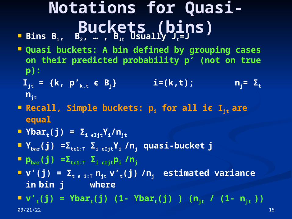
Notations for Quasi-Buckets (bins)

Bins B1, B2, … , BJt Usually Jt=J Quasi buckets: A bin defined by grouping

cases on their predicted probability p’ (not on true p):

Ijt = {k, p’k,t є Bj} i=(k,t); nj= Σt njt

Recall, Simple buckets: pi for all iє Ijt are equal

Ybart(j) = Σi єIjtYi/njt Ybar(j) =Σtє1:T Σi єIjtYi /nj quasi-bucket j pbar(j) =Σtє1:T Σi єIjtpi /nj

v’(j) = Σt є 1:T njt v’t(j) /nj estimated variance in

bin j where v’t(j) = Ybart(j) (1- Ybart(j) ) (njt / (1- njt ))

04/18/23 16

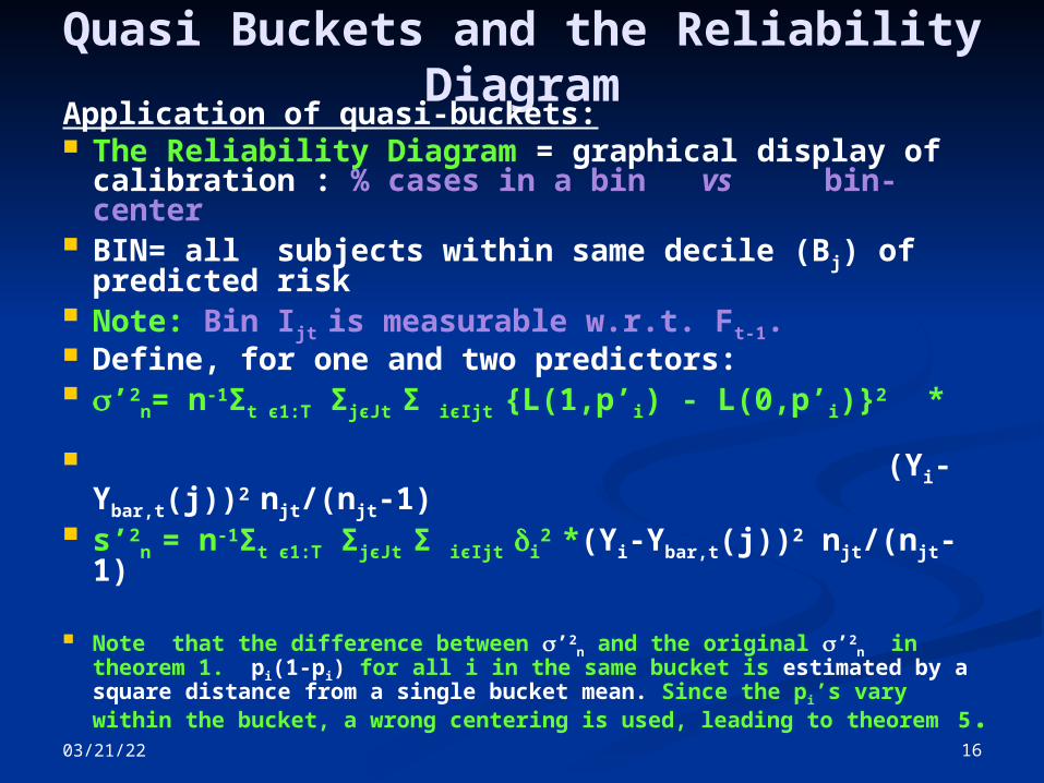
Quasi Buckets and the Reliability Diagram

Application of quasi-buckets: The Reliability Diagram = graphical display of

calibration : % cases in a bin vs bin-center BIN= all subjects within same decile (Bj) of

predicted risk Note: Bin Ijt is measurable w.r.t. Ft-1. Define, for one and two predictors: ’2

n= n-1Σt є1:T ΣjєJt Σ iєIjt {L(1,p’i) - L(0,p’i)}2 *

(Yi-Ybar,t(j))2 njt/(njt-1) s’2

n = n-1Σt є1:T ΣjєJt Σ iєIjt i2 *(Yi-Ybar,t(j))2 njt/(njt-1)

Note that the difference between ’2n and the original ’2

n in theorem 1. pi(1-pi) for all i in the same bucket is estimated by a square distance from a single bucket mean. Since the pi’s vary within the bucket, a wrong centering is used, leading to theorem 5.

04/18/23 17

The simulation t=1,2 Jt=5 Bin(j) = ((j-1)/5, j/5) j=1,…,5 True probabilities: pjt ~ Unif(Bin(j)) nj=30 for j=1,…,5 Simulate: 1. Table of true and estimated

bucket variances 2. Reliability diagram using

confidence intervals from Theorem 5

04/18/23 18

Simulated Reliability Diagram

04/18/23 19

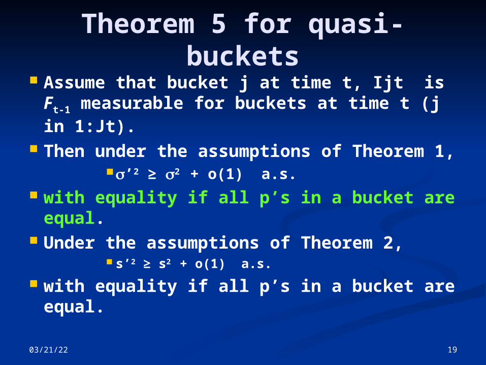
Theorem 5 for quasi-buckets

Assume that bucket j at time t, Ijt is Ft-1 measurable for buckets at time t (j in 1:Jt).

Then under the assumptions of Theorem 1,

’2 ≥ 2 + o(1) a.s. with equality if all p’s in a bucket are

equal. Under the assumptions of Theorem 2,

s’2 ≥ s2 + o(1) a.s.

with equality if all p’s in a bucket are equal.

04/18/23 20

Quasi-buckets Theorem 5 continued

If nj/n converges in probability to a positive constant, and

v(j) = Σt є 1:T Σi є Ijt pi(1-pi) /nj

Then (nj/v(j))1/2 (Ybar(j) – pbar(j)) converges in distribution to N(0,1) and

v’(j) ≥ v(j) +op(1)

04/18/23 21

Simulation results for a 5 bucket

example Min Q1 Q2 Q3 Max Mean SD pbar(2) 0.101 0.300 0.300 0.355 0.515 0.320 0.049

Ybar(2) 0.050 0.267 0.317 0.378 0.633 0.319 0.089 v(2) 0.087 0.207 0.207 0.207 0.247 0.209 0.015 v’(2) 0.048 0.208 0.221 0.239 0.259 0.213 0.034Pbar(5) 0.769 0.906 0.906 0.906 0.906 0.895 0.026

Ybar(5) 0.733 0.867 0.900 0.933 1.000 0.892 0.049 v(5) 0.082 0.082 0.082 0.082 0.164 0.088 0.016 v’(5) 0.077 0.084 0.093 0.120 0.202 0.096 0.037

04/18/23 22

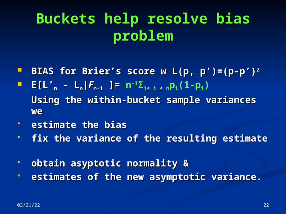
Buckets help resolve bias Buckets help resolve bias problemproblem

BIAS for Brier’s score w L(p, p’)=(p-p’)BIAS for Brier’s score w L(p, p’)=(p-p’)2 2

E[L’E[L’nn – L – Lnn||FFn-1n-1 ]= ]= n-1Σ1≤ ≤ i ≤≤ npi(1-pi)

Using the within-bucket sample variances Using the within-bucket sample variances we we

estimate the biasestimate the bias fix the variance of the resulting estimate fix the variance of the resulting estimate obtain asyptotic normality &obtain asyptotic normality & estimates of the new asymptotic variance.estimates of the new asymptotic variance.

04/18/23 23

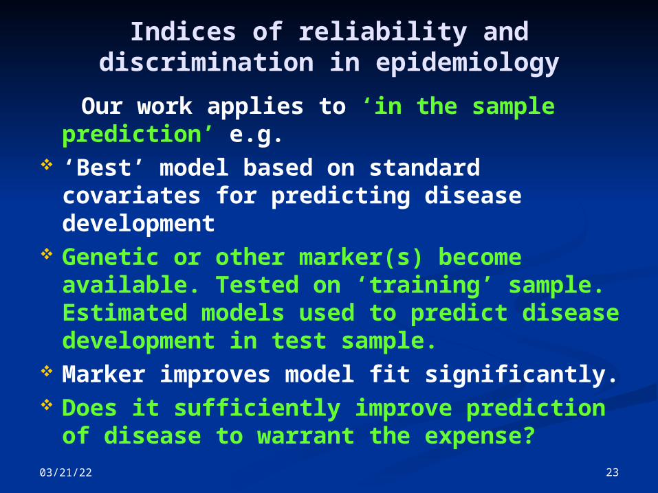
Indices of reliability and discrimination in epidemiology

Our work applies to ‘in the sample prediction’ e.g.

‘Best’ model based on standard covariates for predicting disease development

Genetic or other marker(s) become available. Tested on ‘training’ sample. Estimated models used to predict disease development in test sample.

Marker improves model fit significantly. Does it sufficiently improve prediction of

disease to warrant the expense?

04/18/23 24

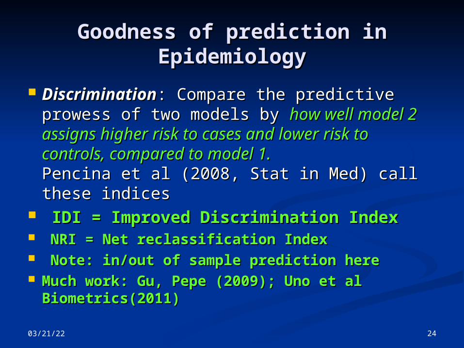
Goodness of prediction in Goodness of prediction in EpidemiologyEpidemiology

DiscriminationDiscrimination: Compare the predictive : Compare the predictive prowess of two models by prowess of two models by how well model 2 how well model 2 assigns higher risk to cases and lower risk to assigns higher risk to cases and lower risk to controls, compared to model 1.controls, compared to model 1. Pencina et al (2008, Stat in Med) call these Pencina et al (2008, Stat in Med) call these indicesindices

IDI = Improved Discrimination IndexIDI = Improved Discrimination Index NRI = Net reclassification IndexNRI = Net reclassification Index Note: in/out of sample prediction hereNote: in/out of sample prediction here Much work: Gu, Pepe (2009); Uno et al Much work: Gu, Pepe (2009); Uno et al

Biometrics(2011)Biometrics(2011)

04/18/23 25

Current work and Current work and simulationssimulations

Martingale approach applies to “out of the sample” Martingale approach applies to “out of the sample” evaluation of indices like NRI and IDI, AUC, and Revaluation of indices like NRI and IDI, AUC, and R2 2

differences.differences. For Epidemiological applications, For Epidemiological applications, in the sample model in the sample model

comparison for predictioncomparison for prediction, assuming: , assuming: ((Y, ZY, Z) iid () iid (responseresponse indicator, covariate vector)indicator, covariate vector) neither model is necessarily the true modelneither model is necessarily the true model models differ by one or more covariates.models differ by one or more covariates. larger model significantly better than smaller modellarger model significantly better than smaller model logistic or similar models,logistic or similar models,

parameters of both models estimated by MLEparameters of both models estimated by MLE we proved asymptotic normality, and provided variance we proved asymptotic normality, and provided variance

estimates, for the IDI and Brier score difference.estimates, for the IDI and Brier score difference.

IDIIDI2/12/1= E[p’’-p’|Y=1] - E[p’’-p’|Y=0] = E[p’’-p’|Y=1] - E[p’’-p’|Y=0] BRI=BR(1)-BR(2)BRI=BR(1)-BR(2) Simulation resultsSimulation results Real data from a French Dementia study.Real data from a French Dementia study.

04/18/23 26

On the Three City Study Cohort study. Purpose: Identify variables that help predict

dementia in people over 65. Our sample: n = 4214 individuals. 162

developed Dementia within 4 years. http://www.three-city-study.com/baseline-characteri

stics-of-the-3c-cohort.php

Ages: 65-74 55% Educ: Primary School 33%

75-79 27% High School 43% 80+ 17% Beyond HS

24% Original data: Gender Men 3650 Women

5644 at start

04/18/23 27

Three City Occupation & Income

Occupation Men (%) Women (%)

SENIOR EXEC 33 11MID EXEC 24 18OFFICE WORKER 14 38SKILLED WORKER 29 17HOUSEWIFE 16Annual Income>2300 Euro 45 241000-2300 29 25750-1000 19 36<750 2 8

04/18/23 28

The predictive model w Marker

TABLE V

LOGISTIC MODEL 1 INCLUDING THE GENETIC MARKER APOE4. Estimate Std. Error Pr(>|z|) (Intercept) -2.944 0.176 < 2e-16 age.fac.31 -2.089 0.330 2.3e-10 age.fac.32 -0.984 0.191 2.5e-07 Education -0.430 0.180 0.0167 Cardio 0.616 0.233 0.0081 Depress 0.786 0.201 9.5e-05 incap 1.180 0.206 1.1e-08 APOE4 0.634 0.195 0.0012 AIC = 1002 Age1: 65<71. Age2 71 <78

04/18/23 29

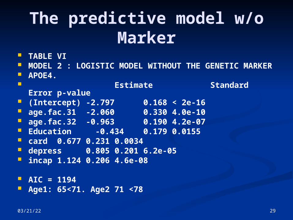
The predictive model w/o Marker

TABLE VI MODEL 2 : LOGISTIC MODEL WITHOUT THE GENETIC

MARKER APOE4. Estimate Standard Error

p-value (Intercept) -2.797 0.168 < 2e-16 age.fac.31 -2.060 0.330 4.0e-10 age.fac.32 -0.963 0.190 4.2e-07 Education -0.434 0.179 0.0155 card 0.677 0.231 0.0034 depress 0.805 0.201 6.2e-05 incap 1.124 0.206 4.6e-08

AIC = 1194 Age1: 65<71. Age2 71 <78

04/18/23 30

The Bootstrap and Our Estimates

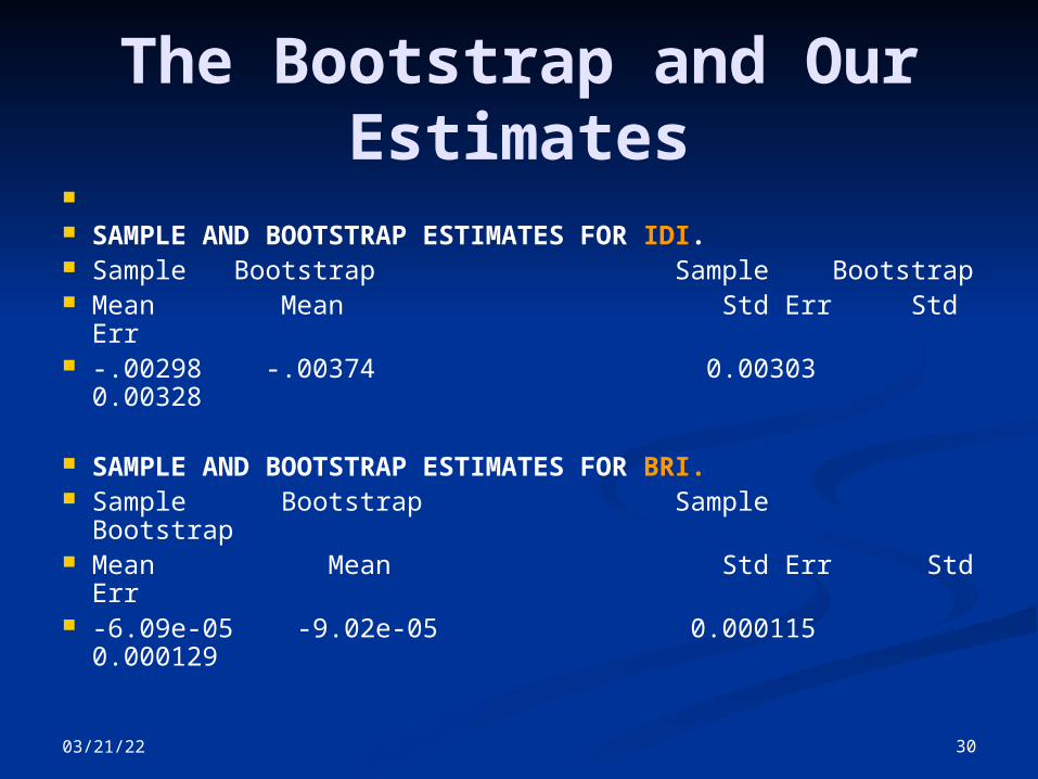
SAMPLE AND BOOTSTRAP ESTIMATES FOR IDI. Sample Bootstrap Sample Bootstrap Mean Mean Std Err Std Err -.00298 -.00374 0.00303 0.00328

SAMPLE AND BOOTSTRAP ESTIMATES FOR BRI. Sample Bootstrap Sample Bootstrap Mean Mean Std Err Std Err -6.09e-05 -9.02e-05 0.000115 0.000129

04/18/23 31

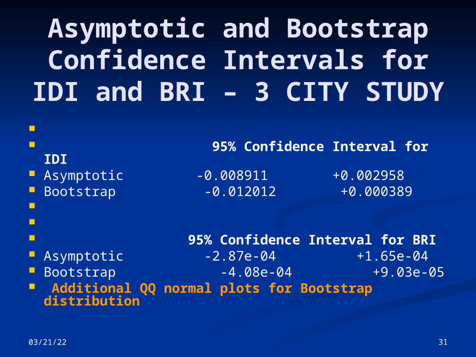
Asymptotic and Bootstrap Confidence Intervals for IDI

and BRI – 3 CITY STUDY 95% Confidence Interval for IDI Asymptotic -0.008911 +0.002958 Bootstrap -0.012012 +0.000389 95% Confidence Interval for BRI Asymptotic -2.87e-04 +1.65e-04 Bootstrap -4.08e-04 +9.03e-05 Additional QQ normal plots for Bootstrap

distribution

04/18/23 32

Discussion and Summary We have provided a probabilistic setting for

inference on prediction scores and provided asymptotic results for discrimination and accuracy measures prevalent in life sciences in within the sample prediction .

In-sample prediction: Assumed chosen models need not coincide with true model. Obtain Asymptotics for IDI and BRI. Convergence is slow for models for which true coefficients are small.

We considered predicting P[event] only. Different problems pop up for prediction of a discrete probability distribution. Certainly our setting can be used but scores have to be carefully chosen.

What about predicting ranks? (Sports. Internet search engines)