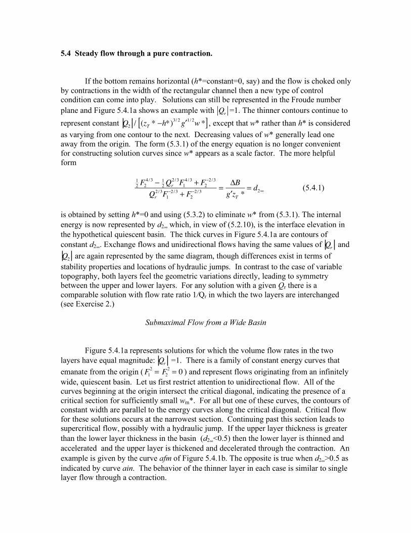
5.4 Steady flow through a pure contraction. If the bottom remains horizontal (h*=constant=0, say) and the flow is choked only by contractions in the width of the rectangular channel then a new type of control condition can come into play. Solutions can still be represented in the Froude number plane and Figure 5.4.1a shows an example with Q

r=1. The thinner contours continue to

represent constant Q2/ (zT * !h*)

3/ 2" g 1/ 2

w *[ ] , except that w* rather than h* is considered as varying from one contour to the next. Decreasing values of w* generally lead one away from the origin. The form (5.3.1) of the energy equation is no longer convenient for constructing solution curves since w* appears as a scale factor. The more helpful form

1

2F2

4 /3!

1

2Qr

2 /3F1

4 /3+ F

2

!2 /3

Qr

2 /3F1

!2 /3+ F

2

!2 /3=

"B

#g zT *= d

2$ (5.4.1)

is obtained by setting h*=0 and using (5.3.2) to eliminate w* from (5.3.1). The internal energy is now represented by d2∞ which, in view of (5.2.10), is the interface elevation in the hypothetical quiescent basin. The thick curves in Figure 5.4.1a are contours of constant d2∞. Exchange flows and unidirectional flows having the same values of Q

r and

Q2

are again represented by the same diagram, though differences exist in terms of stability properties and locations of hydraulic jumps. In contrast to the case of variable topography, both layers feel the geometric variations directly, leading to symmetry between the upper and lower layers. For any solution with a given Qr there is a comparable solution with flow rate ratio 1/Qr in which the two layers are interchanged (see Exercise 2.)

Submaximal Flow from a Wide Basin Figure 5.4.1a represents solutions for which the volume flow rates in the two layers have equal magnitude: Q

r =1. There is a family of constant energy curves that

emanate from the origin (F1

2

= F2

2

= 0 ) and represent flows originating from an infinitely wide, quiescent basin. Let us first restrict attention to unidirectional flow. All of the curves beginning at the origin intersect the critical diagonal, indicating the presence of a critical section for sufficiently small wm*. For all but one of these curves, the contours of constant width are parallel to the energy curves along the critical diagonal. Critical flow for these solutions occurs at the narrowest section. Continuing past this section leads to supercritical flow, possibly with a hydraulic jump. If the upper layer thickness is greater than the lower layer thickness in the basin (d2∞<0.5) then the lower layer is thinned and accelerated and the upper layer is thickened and decelerated through the contraction. An example is given by the curve afm of Figure 5.4.1b. The opposite is true when d2∞>0.5 as indicated by curve ain. The behavior of the thinner layer in each case is similar to single layer flow through a contraction.

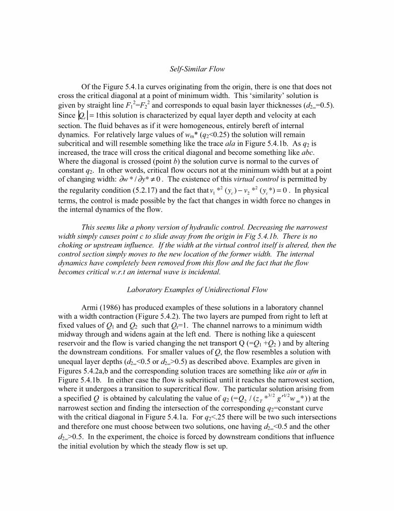
Self-Similar Flow Of the Figure 5.4.1a curves originating from the origin, there is one that does not cross the critical diagonal at a point of minimum width. This ‘similarity’ solution is given by straight line F1

2=F22 and corresponds to equal basin layer thicknesses (d2∞=0.5).

Since Qr= 1this solution is characterized by equal layer depth and velocity at each

section. The fluid behaves as if it were homogeneous, entirely bereft of internal dynamics. For relatively large values of wm* (q2<0.25) the solution will remain subcritical and will resemble something like the trace ala in Figure 5.4.1b. As q2 is increased, the trace will cross the critical diagonal and become something like abc. Where the diagonal is crossed (point b) the solution curve is normal to the curves of constant q2. In other words, critical flow occurs not at the minimum width but at a point of changing width: !w * /!y* " 0 . The existence of this virtual control is permitted by the regularity condition (5.2.17) and the fact thatv

1*2(y

c) ! v

2*2(y

c*) = 0 . In physical

terms, the control is made possible by the fact that changes in width force no changes in the internal dynamics of the flow. This seems like a phony version of hydraulic control. Decreasing the narrowest width simply causes point c to slide away from the origin in Fig 5.4.1b. There is no choking or upstream influence. If the width at the virtual control itself is altered, then the control section simply moves to the new location of the former width. The internal dynamics have completely been removed from this flow and the fact that the flow becomes critical w.r.t an internal wave is incidental.

Laboratory Examples of Unidirectional Flow Armi (1986) has produced examples of these solutions in a laboratory channel with a width contraction (Figure 5.4.2). The two layers are pumped from right to left at fixed values of Q1 and Q2 such that Qr=1. The channel narrows to a minimum width midway through and widens again at the left end. There is nothing like a quiescent reservoir and the flow is varied changing the net transport Q (=Q1 +Q2 ) and by altering the downstream conditions. For smaller values of Q, the flow resembles a solution with unequal layer depths (d2∞<0.5 or d2∞>0.5) as described above. Examples are given in Figures 5.4.2a,b and the corresponding solution traces are something like ain or afm in Figure 5.4.1b. In either case the flow is subcritical until it reaches the narrowest section, where it undergoes a transition to supercritical flow. The particular solution arising from a specified Q is obtained by calculating the value of q2 (=Q

2/ (zT *

3/2! g 1/ 2

w m*)) at the narrowest section and finding the intersection of the corresponding q2=constant curve with the critical diagonal in Figure 5.4.1a. For q2<.25 there will be two such intersections and therefore one must choose between two solutions, one having d2∞<0.5 and the other d2∞>0.5. In the experiment, the choice is forced by downstream conditions that influence the initial evolution by which the steady flow is set up.

If Q is increased, the value of q2 at the narrowest section increases, forcing the intersection with the critical diagonal to move closer to the midpoint F1

2= F22=1/2. The

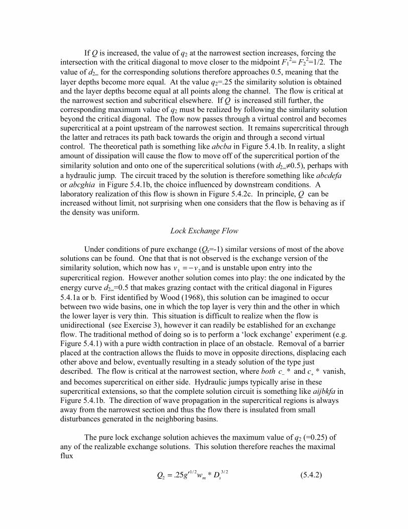
value of d2∞ for the corresponding solutions therefore approaches 0.5, meaning that the layer depths become more equal. At the value q2=.25 the similarity solution is obtained and the layer depths become equal at all points along the channel. The flow is critical at the narrowest section and subcritical elsewhere. If Q is increased still further, the corresponding maximum value of q2 must be realized by following the similarity solution beyond the critical diagonal. The flow now passes through a virtual control and becomes supercritical at a point upstream of the narrowest section. It remains supercritical through the latter and retraces its path back towards the origin and through a second virtual control. The theoretical path is something like abcba in Figure 5.4.1b. In reality, a slight amount of dissipation will cause the flow to move off of the supercritical portion of the similarity solution and onto one of the supercritical solutions (with d2∞≠0.5), perhaps with a hydraulic jump. The circuit traced by the solution is therefore something like abcdefa or abcghia in Figure 5.4.1b, the choice influenced by downstream conditions. A laboratory realization of this flow is shown in Figure 5.4.2c. In principle, Q can be increased without limit, not surprising when one considers that the flow is behaving as if the density was uniform.

Lock Exchange Flow Under conditions of pure exchange (Qr=-1) similar versions of most of the above solutions can be found. One that that is not observed is the exchange version of the similarity solution, which now has v

1= !v

2and is unstable upon entry into the

supercritical region. However another solution comes into play: the one indicated by the energy curve d2∞=0.5 that makes grazing contact with the critical diagonal in Figures 5.4.1a or b. First identified by Wood (1968), this solution can be imagined to occur between two wide basins, one in which the top layer is very thin and the other in which the lower layer is very thin. This situation is difficult to realize when the flow is unidirectional (see Exercise 3), however it can readily be established for an exchange flow. The traditional method of doing so is to perform a ‘lock exchange’ experiment (e.g. Figure 5.4.1) with a pure width contraction in place of an obstacle. Removal of a barrier placed at the contraction allows the fluids to move in opposite directions, displacing each other above and below, eventually resulting in a steady solution of the type just described. The flow is critical at the narrowest section, where both c

!* and c

+* vanish,

and becomes supercritical on either side. Hydraulic jumps typically arise in these supercritical extensions, so that the complete solution circuit is something like aijbkfa in Figure 5.4.1b. The direction of wave propagation in the supercritical regions is always away from the narrowest section and thus the flow there is insulated from small disturbances generated in the neighboring basins. The pure lock exchange solution achieves the maximum value of q2 (=0.25) of any of the realizable exchange solutions. This solution therefore reaches the maximal flux Q

2= .25 ! g

1/ 2wm * Ds

3/ 2 (5.4.2)

for fixed minimum width wm*. The formula follows from use of the definition of q2 along with its observed value, or simply by setting Q

r=1 in (5.3.4). This solution is

characterized by a double hydraulic control in the sense that both internal waves are frozen at the narrows. Stommel and Farmer (1952) identified this state and verified it experimentally. Their analysis and their later (1953) application to estuary dynamics deserves special mention in the annals of hydraulics. The work revealed the first example of maximal exchange and also represented one of the first applications of hydraulic theory to oceanographically relevant flows. Both layers are engaged: the upper layer being more so in one reservoir, the second in the other, and both being active at the narrowest section. The submaximal solutions (d2∞≠0.5) are characterized by having only one wave frozen at the narrowest section, by having a smaller Q2 for the same wm*, zT* and g′, and by being dominated by the dynamics of one of the layers. For unidirectional flow we do not identify a maximal solution. The ability of the flow to become barotropic means that the volume flux that can be forced through the contraction is unlimited. It is possible to devise a number of experiments demonstrating how maximal flow is obtained as a limiting case of the submaximal flows. For example, one might carry out a series of lock exchange solutions in which the initial barrier extends only partially through the depth. One reservoir is filled to the top with the lighter fluid. The other is filled to the top of the barrier with the denser fluid with the less dense fluid lying above. If this partial barrier is low enough, the exchange flow set up by its removal will be submaximal. Increasing the barrier height sufficiently will eventually lead to formation of the maximal solution. A similar set of experiments could be made by pumping the fluids in opposite directions and gradually increasing the pumping rates. The sequence of exchange solutions that one might encounter is shown in Figure 5.4.3. I need a basic reference here regarding the two-layer lock exchange experiment and how maximal and submaximal flows are produced. Wood 1970 did the right experiment but did not know about submaximal vs. maximal flows and the documentation of his experiments was not very extensive.. Lane-Serff, et al. 2000 did a 3-layer version of the experiment, but it is too advanced. Does anyone reading this know of a good experimental reference?

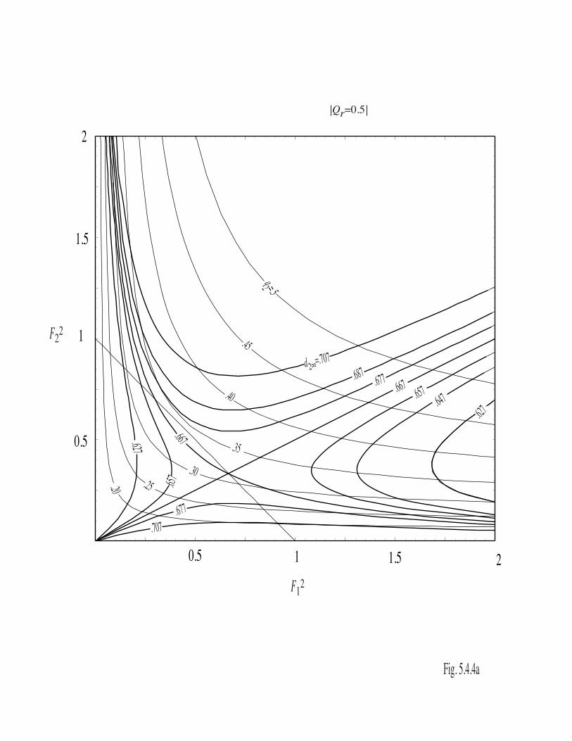
Unequal Layer Fluxes Froude number diagrams for Q

r≠1 show similar features but with a loss of

symmetry between upper and lower layers. The case Qr

=0.5 is shown in Figure 5.4.4a. Under conditions of exchange (Qr<0), the flow contains a barotropic component, equal to Q1+Q2 (=Q1/2). The similarity solution with the virtual control lies along the straight contour with d2∞=2/3. [For general Q

r, the corresponding value of d2∞ is given by

(Qr+ 1)

!1and the contour itself by QrF1

2

= F2

2 .] However, the former ‘lock exchange’ solution, which occurs along the curved energy contour with d2∞=2/3, now has two control sections. The first is a virtual control, which lies at the lower right intersection with the critical diagonal, and a narrows control lying at the upper left intersection. It can be shown that the virtual control lies on the side of the narrows from which the barotropic

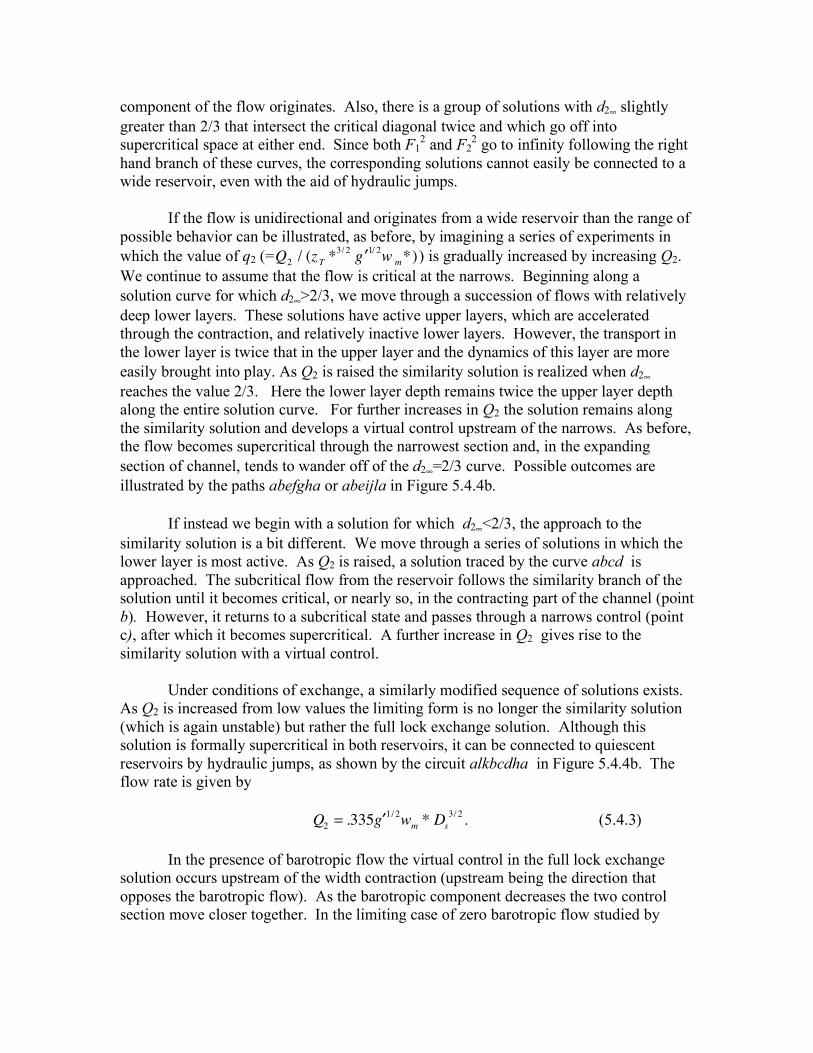
component of the flow originates. Also, there is a group of solutions with d2∞ slightly greater than 2/3 that intersect the critical diagonal twice and which go off into supercritical space at either end. Since both F1

2 and F22 go to infinity following the right

hand branch of these curves, the corresponding solutions cannot easily be connected to a wide reservoir, even with the aid of hydraulic jumps. If the flow is unidirectional and originates from a wide reservoir than the range of possible behavior can be illustrated, as before, by imagining a series of experiments in which the value of q2 (=Q

2/ (zT *

3/2! g 1/ 2

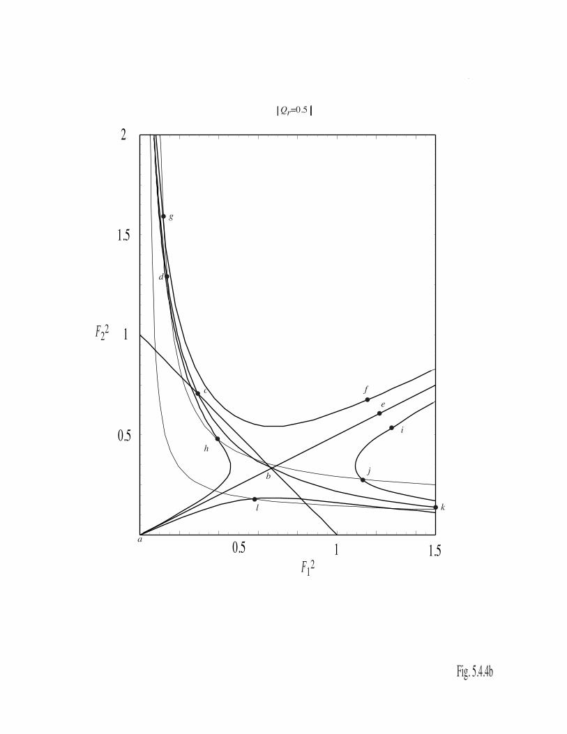
w m*)) is gradually increased by increasing Q2. We continue to assume that the flow is critical at the narrows. Beginning along a solution curve for which d2∞>2/3, we move through a succession of flows with relatively deep lower layers. These solutions have active upper layers, which are accelerated through the contraction, and relatively inactive lower layers. However, the transport in the lower layer is twice that in the upper layer and the dynamics of this layer are more easily brought into play. As Q2 is raised the similarity solution is realized when d2∞ reaches the value 2/3. Here the lower layer depth remains twice the upper layer depth along the entire solution curve. For further increases in Q2 the solution remains along the similarity solution and develops a virtual control upstream of the narrows. As before, the flow becomes supercritical through the narrowest section and, in the expanding section of channel, tends to wander off of the d2∞=2/3 curve. Possible outcomes are illustrated by the paths abefgha or abeijla in Figure 5.4.4b. If instead we begin with a solution for which d2∞<2/3, the approach to the similarity solution is a bit different. We move through a series of solutions in which the lower layer is most active. As Q2 is raised, a solution traced by the curve abcd is approached. The subcritical flow from the reservoir follows the similarity branch of the solution until it becomes critical, or nearly so, in the contracting part of the channel (point b). However, it returns to a subcritical state and passes through a narrows control (point c), after which it becomes supercritical. A further increase in Q2 gives rise to the similarity solution with a virtual control. Under conditions of exchange, a similarly modified sequence of solutions exists. As Q2 is increased from low values the limiting form is no longer the similarity solution (which is again unstable) but rather the full lock exchange solution. Although this solution is formally supercritical in both reservoirs, it can be connected to quiescent reservoirs by hydraulic jumps, as shown by the circuit alkbcdha in Figure 5.4.4b. The flow rate is given by Q

2= .335 ! g

1/ 2wm * Ds

3/ 2 . (5.4.3)

In the presence of barotropic flow the virtual control in the full lock exchange solution occurs upstream of the width contraction (upstream being the direction that opposes the barotropic flow). As the barotropic component decreases the two control section move closer together. In the limiting case of zero barotropic flow studied by

Stommel and Farmer (1952, 1953) the virtual control is hidden by the fact that the two controls occur together. For further reading on the subject of two-layer flow, one could consult Baines (1995), the work of Armi and Farmer as referenced in their 1988 paper. Exercises 1) By free hand, sketch the qualitative features of the solutions corresponding to the following circuits: a) afm (Figure 5.4.1b) b) ain (Figure 5.4.1b) c) abcba (Figure 5.4.1b) d) jbk (Figure 5.4.1b) e) aijbkfa (Figure 5.4.1b) f) kbcd (Figure 5.4.4b) g) alkbcdha (Figure 5.4.4b) The sketches should be the style of the Figure 5.3.1b insets, with control sections and stretches of subcritical and supercritical flow labeled. 2) For flow through a contraction with constant h*, show that for each Qr there is another solution with reciprocal flow rate ratio (1/Qr) in which the two layers are interchanged. 3) Consider the following flows, each of which has at least one critical section. Remark on the stability of the hydraulic transition at the critical section(s) in each case. (Speak to the shock-forming instability, not Kelvin-Helmholtz instability.) (a) The solution kjk in Figure 5.4.1b. (b) A solution of the type abcd in Figure 5.4.1a, with the lower layer entering the deep basin and the upper layer exiting the basin. (c) The ‘lock exchange’ solution with Qr=0.5. In other words, the solution with both a virtual and narrows control lying along the d1∞=.667 curve in Figure 5.4.1a, but now with unidirectional flow. 4) Verify (5.4.3) by direct calculation (i.e. do not use the contour values printed on the curves in Figure 5.4.4a).

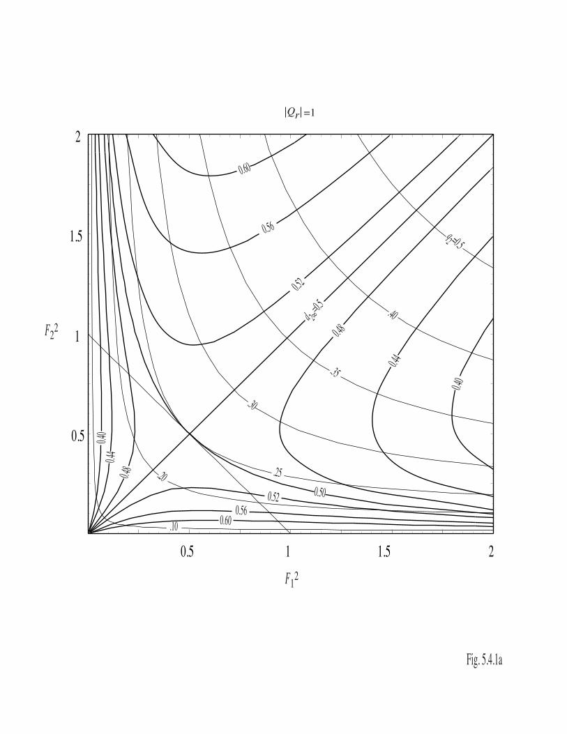
Figure Captions Figure 5.4.1a The Froude number plane for flow through a pure contraction with Q

r=1.

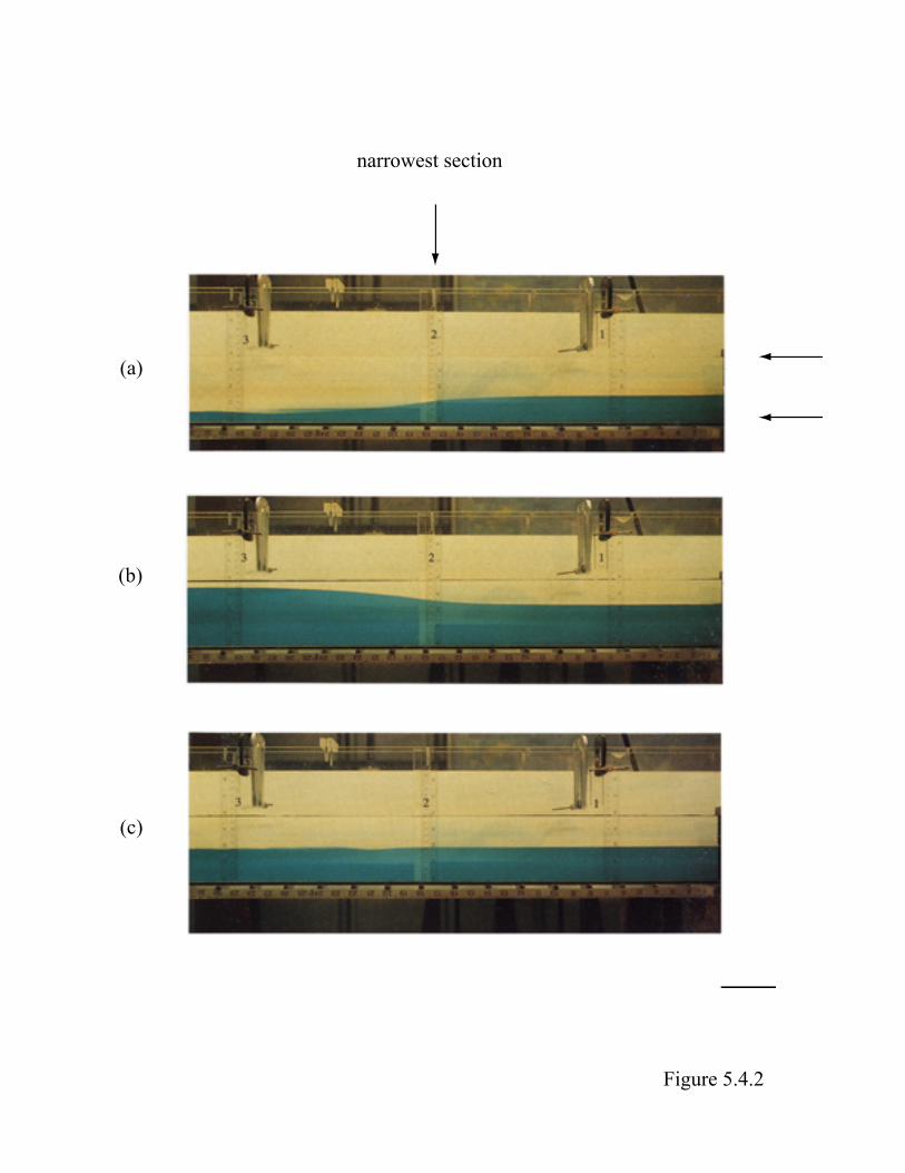
Solutions must lie along the thick curves, which have constant d2∞. The thin curves are of constant q2 and are the same as in Figure 5.3.1a, but now the larger values of this parameter are associated with narrower widths. Figure 5.4.1b Examples of solutions for the previous figure, as described in the text. Figure 5.4.2 Side views of unidirectional, two-layer flows through a contraction. Frames (a) and (b) show flows with a control section at the narrowest section, which lies approximately at the numeral ‘2’. Frame (c) shows a self-similar flow with a virtual control. At the upstream (right) entrance the layer depths and velocities are equal and continue to be so as the channel converges and the narrowest section is passed. The virtual control occurs somewhere to the right of the narrowest section but is not distinguished by any visual property of the interface. A small amount of mixing is observed in the downstream end of the channel. (Based on Plates 1 and 2 from Armi, 1986). Figure 5.4.3. A sequence of steady solutions for two-layer exchange through a pure contraction, as described in the text. (Based on Figure 2 from Armi and Farmer, 1986). Figure 5.4.4a Froude number plane for flow through a pure contraction with Q

r=0.5

Figure 5.4.4b Examples of solutions for previous figures as described in the text.

0.5 1 1.5 2

0.5

1

1.5

2

F12

F22d 2∞=

0.5

Fig. 5.4.1a

0.52

0.48

0.44

0.40

0.56

0.60

0.500.520.56

0.60

0.480.44

0.40

q2 =0.5

.40

.35

.30

.20

.10

.25

Qr =1

F12

F22 d

Fig. 5.4.1b

0.5 1. 1.5

0.5

1.

1.5

j

c

g

e

k

f

i

b

h

a

Qr =1

l

m

n

(a)

(b)

(c)

Figure 5.4.2

narrowest section

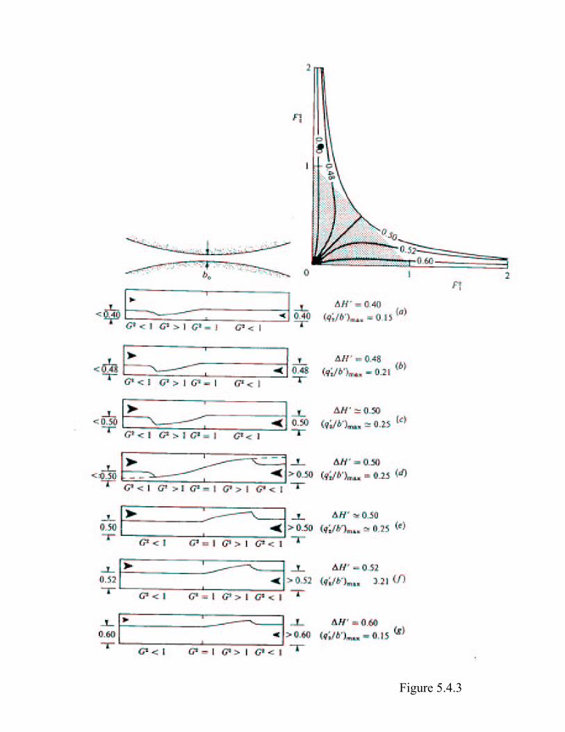
Figure 5.4.3

F12

F22

d 2∞=.707

Fig. 5.4.4a

0.5 1 1.5 2

0.5

1

1.5

2

.687.677

.667.657

.647

.627

q2 =.5

.45

.40

.35.30

.25.20

.677.707

.627

.657

.667

Qr=0.5

F22

f

Fig. 5.4.4b

0.5 1 1.5

2

F12

1.5

0.5

1

g

j

h

ce

i

d

b

a

kl

Qr=0.5