15.16. Eigenvalue and Eigenvector Extraction

The eigenvalue and eigenvector problem needs to be solved for mode-frequency and buckling analyses. It has the form of:

where:

For prestressed modal analyses, the [K] matrix includes the stress stiffness matrix [S]. For eigenvalue buckling analyses, the [M] matrix is replaced with the stress stiffness matrix [S]. The discussions given in the rest of this section assume a modal analysis (ANTYPE,MODAL) except as noted, but also generally applies to eigenvalue buckling analyses.

The eigenvalue and eigenvector extraction procedures available include the reduced, subspace, Block Lanczos, PCG Lanczos, unsymmetric, damped, and QR damped methods (MODOPT and BUCOPT commands) outlined in Table 15.1: "Procedures Used for Eigenvalue and Eigenvector Extraction". The PCG Lanczos method uses Lanczos iterations, but employs the PCG solver. Each method is discussed subsequently. Shifting, applicable to all methods, is discussed at the end of this section.

Table 15.1 Procedures Used for Eigenvalue and Eigenvector Extraction

The PCG Lanczos method is the same as the Block Lanczos method, except it uses the iterative solver instead of the sparse direct equation solver to solve.

15.16.1. Reduced Method

(15–180)

[K] = structure stiffness matrix {φi} = eigenvector

λi = eigenvalue

[M] = structure mass matrix

Procedure Input Usages Applicable Matrices++

Reduction Extraction Technique

Reduced MODOPT, REDUC Any (but not recommended for buckling)

K, M Guyan HBI

Subspace MODOPT, SUBSP Symmetric K, M None Subspace which internally uses Jacobi

Block Lanczos MODOPT, LANB Symmetric K, M None Lanczos which internally uses QL algorithm

PCG Lanczos MODOPT, LANPCG

Symmetric (but not applicable for buckling)

K, M None Lanczos which internally uses QL algorithm

Unsymmetric MODOPT, UNSYM

Unsymmetric matrices

K*, M* None Lanczos which internally uses QR algorithm

Damped MODOPT, DAMP Symmetric or unsymmetric damped systems

K*, C*, M* None Lanczos which internally uses QR algorithm

QR Damped MODOPT, QRDAMP

Symmetric or unsymmetric damped systems

K*, C*, M* Modal QR algorithm for reduced modal damping matrix

++ K = stiffness matrix, C = damping matrix, M = mass or stress stiffening matrix, * = can be unsymmetric

Theory Reference | Chapter 15. Analysis Tools |

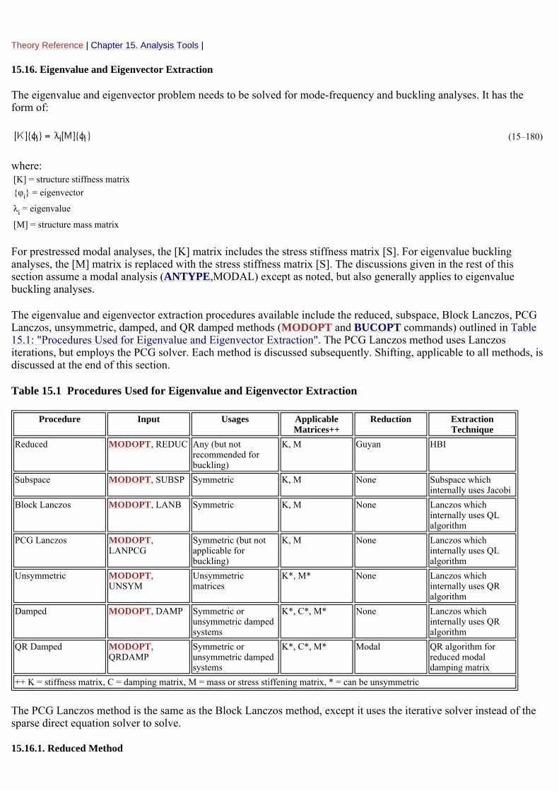
For the reduced procedure (accessed with MODOPT,REDUC), the system of equations is first condensed down to those DOFs associated with the master DOFs by Guyan reduction. This condensation procedure is discussed in Substructuring Analysis ((Equation 17–98) and (Equation 17–110)). The set of n master DOFs characterize the natural frequencies of interest in the system. The selection of the master DOFs is discussed in more detail in Automatic Master DOF Selection of this manual and in Modal Analysis of the Structural Analysis Guide. This technique preserves the potential energy of the system but modifies, to some extent, the kinetic energy. The kinetic energy of the low frequency modes is less sensitive to the condensation than the kinetic energy of the high frequency modes. The number of master DOFs selected should usually be at least equal to twice the number of frequencies of interest. This reduced form may be expressed as:

where:

Next, the actual eigenvalue extraction is performed. The extraction technique employed is the HBI (Householder-Bisection-Inverse iteration) extraction technique and consists of the following five steps:

15.16.1.1. Transformation of the Generalized Eigenproblem to a Standard Eigenproblem

(Equation 15–181) must be transformed to the desired form which is the standard eigenproblem (with [A] being symmetric):

This is accomplished by the following steps:

Premultiply both sides of (Equation 15–181) by :

Decompose into [L][L]T by Cholesky decomposition, where [L] is a lower triangular matrix. Combining with (Equation 15–183),

It is convenient to define:

Combining (Equation 15–184) and (Equation 15–185)), and reducing yields:

(15–181)

= reduced stiffness matrix (known)

= eigenvector (unknown) λi = eigenvalue (unknown)

= reduced mass matrix (known)

(15–182)

(15–183)

(15–184)

(15–185)

(15–186)

or

where:

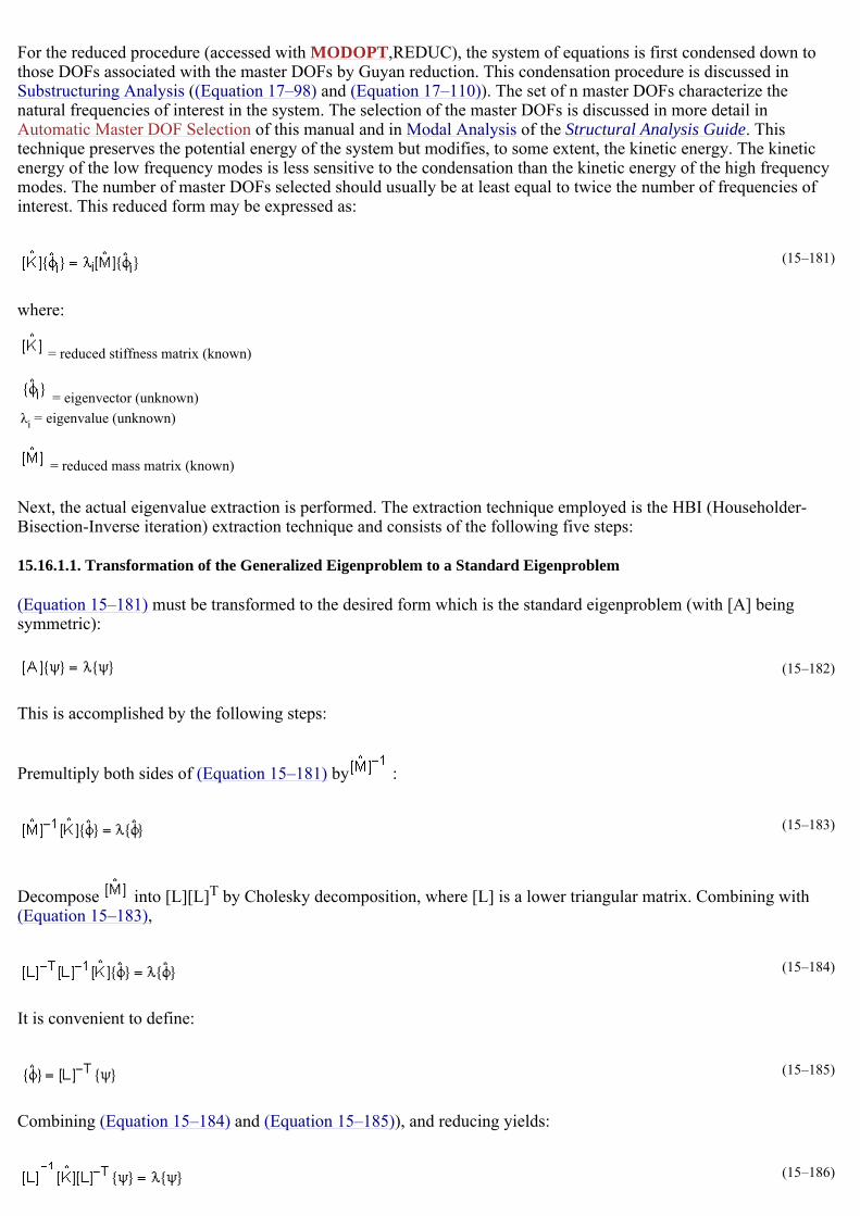
Note that the symmetry of [A] has been preserved by this procedure.

15.16.1.2. Reduce [A] to Tridiagonal Form

This step is performed by Householder's method through a series of similarity transformations yielding

where:

The eigenproblem is reduced to:

Note that the eigenvalues (λ) have not changed through these transformations, but the eigenvectors are related by:

15.16.1.3. Eigenvalue Calculation

Use Sturm sequence checks with the bisection method to determine the eigenvalues.

15.16.1.4. Eigenvector Calculation

The eigenvectors are evaluated using inverse iteration with shifting. The eigenvectors associated with multiple eigenvalues are evaluated using initial vector deflation by Gram-Schmidt orthogonalization in the inverse iteration procedure.

15.16.1.5. Eigenvector Transformation

After the eigenvectors Ψi are evaluated, mode shapes are recovered through (Equation 15–190).

In the expansion pass, the eigenvectors are expanded from the master DOFs to the total DOFs.

15.16.2. Subspace Method

The subspace iteration method (accessed with MODOPT,SUBSP or BUCOPT,SUBSP) is described in detail by Bathe(2). Enhancements as suggested by Wilson and Itoh(166) are also included as outlined subsequently. The basic algorithm consists of the following steps:

1. Define the initial shift s:

In a modal analysis (ANTYPE,MODAL), s = FREQB on the MODOPT command (defaults to -4π2).

(15–187)

(15–188)

[B] = tridiagonalized form of [A][T] = matrix constructed to tridiagonalize [A], solved for iteratively (Bathe(2))

(15–189)

(15–190)

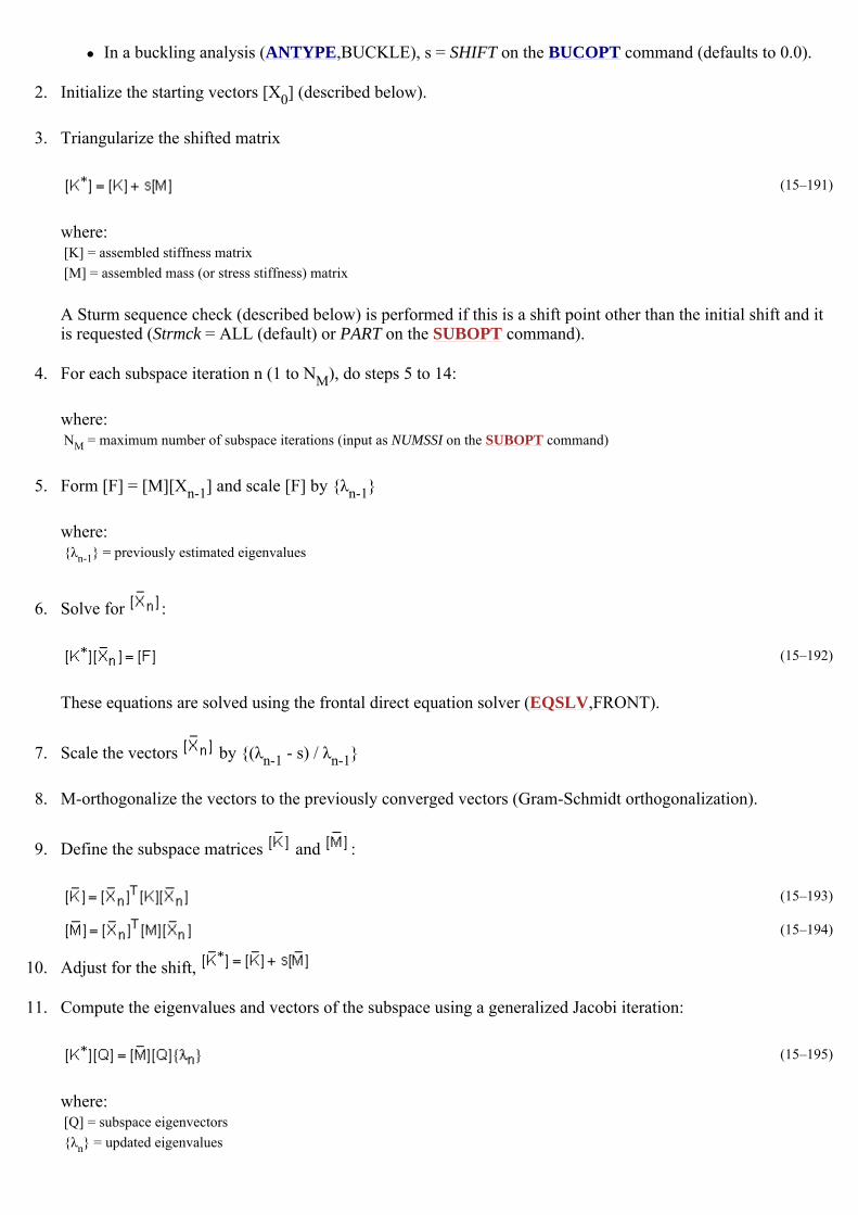
In a buckling analysis (ANTYPE,BUCKLE), s = SHIFT on the BUCOPT command (defaults to 0.0).

2. Initialize the starting vectors [X0] (described below).

3. Triangularize the shifted matrix

where:

A Sturm sequence check (described below) is performed if this is a shift point other than the initial shift and it is requested (Strmck = ALL (default) or PART on the SUBOPT command).

4. For each subspace iteration n (1 to NM), do steps 5 to 14:

where:

5. Form [F] = [M][Xn-1] and scale [F] by {λn-1}

where:

6. Solve for :

These equations are solved using the frontal direct equation solver (EQSLV,FRONT).

7. Scale the vectors by {(λn-1 - s) / λn-1}

8. M-orthogonalize the vectors to the previously converged vectors (Gram-Schmidt orthogonalization).

9. Define the subspace matrices and :

10. Adjust for the shift,

11. Compute the eigenvalues and vectors of the subspace using a generalized Jacobi iteration:

where:

(15–191)

[K] = assembled stiffness matrix [M] = assembled mass (or stress stiffness) matrix

NM = maximum number of subspace iterations (input as NUMSSI on the SUBOPT command)

{λn-1} = previously estimated eigenvalues

(15–192)

(15–193)

(15–194)

(15–195)

[Q] = subspace eigenvectors {λn} = updated eigenvalues

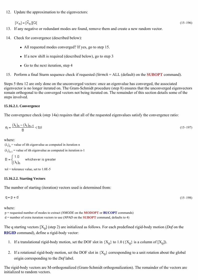
12. Update the approximation to the eigenvectors:

13. If any negative or redundant modes are found, remove them and create a new random vector.

14. Check for convergence (described below):

All requested modes converged? If yes, go to step 15.

If a new shift is required (described below), go to step 3

Go to the next iteration, step 4

15. Perform a final Sturm sequence check if requested (Strmck = ALL (default) on the SUBOPT command).

Steps 5 thru 12 are only done on the unconverged vectors: once an eigenvalue has converged, the associated eigenvector is no longer iterated on. The Gram-Schmidt procedure (step 8) ensures that the unconverged eigenvectors remain orthogonal to the converged vectors not being iterated on. The remainder of this section details some of the steps involved.

15.16.2.1. Convergence

The convergence check (step 14a) requires that all of the requested eigenvalues satisfy the convergence ratio:

where:

15.16.2.2. Starting Vectors

The number of starting (iteration) vectors used is determined from:

where:

The q starting vectors [X0] (step 2) are initialized as follows. For each predefined rigid-body motion (Dof on the RIGID command), define a rigid-body vector:

1. If a translational rigid-body motion, set the DOF slot in {X0} to 1.0 ({X0} is a column of [X0]).

2. If a rotational rigid-body motion, set the DOF slot in {X0} corresponding to a unit rotation about the global origin corresponding to the Dof label.

The rigid-body vectors are M-orthogonalized (Gram-Schmidt orthogonalization). The remainder of the vectors are initialized to random vectors.

(15–196)

(15–197)

(λi)n = value of ith eigenvalue as computed in iteration n

(λi)n-1 = value of ith eigenvalue as computed in iteration n-1

tol = tolerance value, set to 1.0E-5

(15–198)

p = requested number of modes to extract (NMODE on the MODOPT or BUCOPT commands) d = number of extra iteration vectors to use (NPAD on the SUBOPT command, defaults to 4)

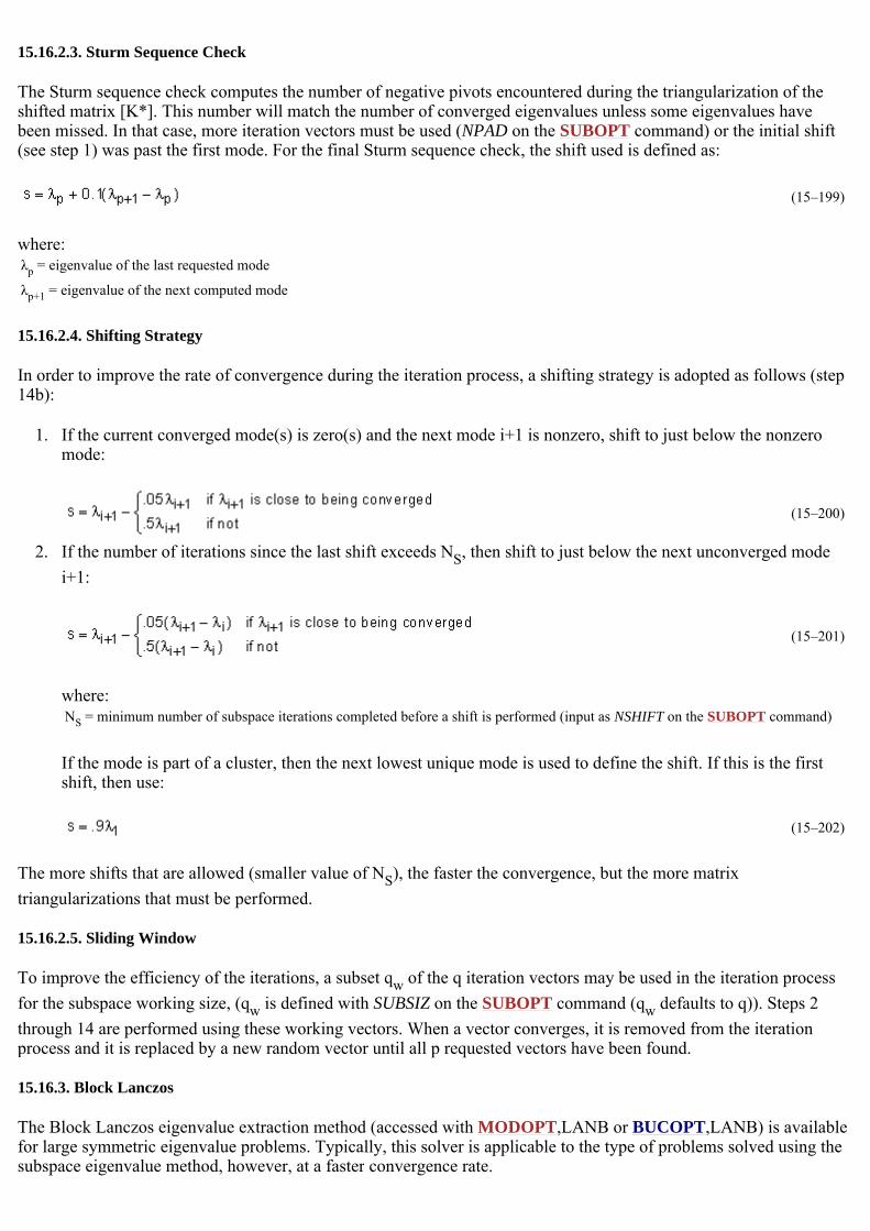
15.16.2.3. Sturm Sequence Check

The Sturm sequence check computes the number of negative pivots encountered during the triangularization of the shifted matrix [K*]. This number will match the number of converged eigenvalues unless some eigenvalues have been missed. In that case, more iteration vectors must be used (NPAD on the SUBOPT command) or the initial shift (see step 1) was past the first mode. For the final Sturm sequence check, the shift used is defined as:

where:

15.16.2.4. Shifting Strategy

In order to improve the rate of convergence during the iteration process, a shifting strategy is adopted as follows (step 14b):

1. If the current converged mode(s) is zero(s) and the next mode i+1 is nonzero, shift to just below the nonzero mode:

2. If the number of iterations since the last shift exceeds NS, then shift to just below the next unconverged mode i+1:

where:

If the mode is part of a cluster, then the next lowest unique mode is used to define the shift. If this is the first shift, then use:

The more shifts that are allowed (smaller value of NS), the faster the convergence, but the more matrix triangularizations that must be performed.

15.16.2.5. Sliding Window

To improve the efficiency of the iterations, a subset qw of the q iteration vectors may be used in the iteration process for the subspace working size, (qw is defined with SUBSIZ on the SUBOPT command (qw defaults to q)). Steps 2 through 14 are performed using these working vectors. When a vector converges, it is removed from the iteration process and it is replaced by a new random vector until all p requested vectors have been found.

15.16.3. Block Lanczos

The Block Lanczos eigenvalue extraction method (accessed with MODOPT,LANB or BUCOPT,LANB) is available for large symmetric eigenvalue problems. Typically, this solver is applicable to the type of problems solved using the subspace eigenvalue method, however, at a faster convergence rate.

(15–199)

λp = eigenvalue of the last requested mode

λp+1 = eigenvalue of the next computed mode

(15–200)

(15–201)

NS = minimum number of subspace iterations completed before a shift is performed (input as NSHIFT on the SUBOPT command)

(15–202)

A block shifted Lanczos algorithm, as found in Grimes et al.(195) is the theoretical basis of the eigensolver. The method used by the modal analysis employs an automated shift strategy, combined with Sturm sequence checks, to extract the number of eigenvalues requested. The Sturm sequence check also ensures that the requested number of eigenfrequencies beyond the user supplied shift frequency (FREQB on the MODOPT command) is found without missing any modes.

The Block Lanczos algorithm is a variation of the classical Lanczos algorithm, where the Lanczos recursions are performed using a block of vectors, as opposed to a single vector. Additional theoretical details on the classical Lanczos method can be found in Rajakumar and Rogers(196).

Use of the Block Lanczos method for solving larger models (500,000 DOF, for example) with many constraint equations (CE) can require a significant amount of computer memory. The alternative method of PCG Lanczos, which internally uses the PCG solver, could result in savings in memory and computing time.

15.16.4. PCG Lanczos

The theoretical basis of this eigensolver is found in Grimes et al.(195), which is the same basis for the Block Lanczos eigenvalue extraction method. However, the implementaion differs somewhat from the Block Lanczos eigensolver, in that the PCG Lanczos eigensolver:

does not change shift values during the eigenvalue analysis.

does not perform a Sturm sequence check by default.

is only available for modal analyses and is not applicable to buckling analyses.

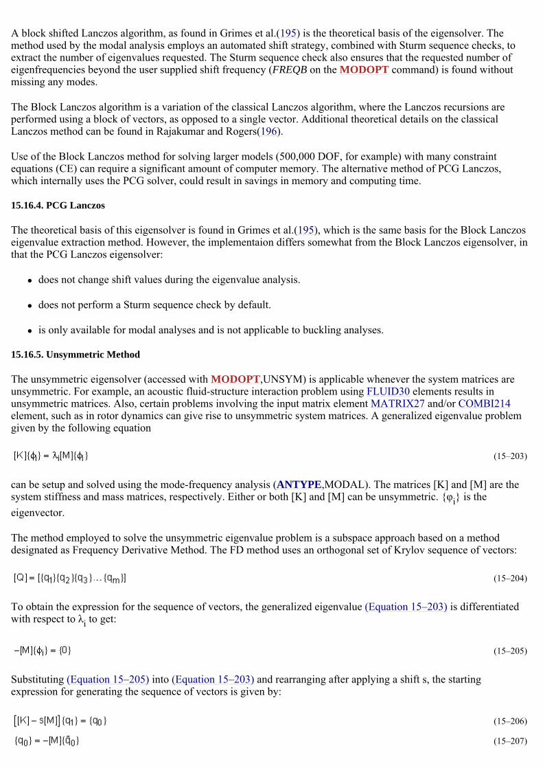
15.16.5. Unsymmetric Method

The unsymmetric eigensolver (accessed with MODOPT,UNSYM) is applicable whenever the system matrices are unsymmetric. For example, an acoustic fluid-structure interaction problem using FLUID30 elements results in unsymmetric matrices. Also, certain problems involving the input matrix element MATRIX27 and/or COMBI214 element, such as in rotor dynamics can give rise to unsymmetric system matrices. A generalized eigenvalue problem given by the following equation

can be setup and solved using the mode-frequency analysis (ANTYPE,MODAL). The matrices [K] and [M] are the system stiffness and mass matrices, respectively. Either or both [K] and [M] can be unsymmetric. {φi} is the eigenvector.

The method employed to solve the unsymmetric eigenvalue problem is a subspace approach based on a method designated as Frequency Derivative Method. The FD method uses an orthogonal set of Krylov sequence of vectors:

To obtain the expression for the sequence of vectors, the generalized eigenvalue (Equation 15–203) is differentiated with respect to λi to get:

Substituting (Equation 15–205) into (Equation 15–203) and rearranging after applying a shift s, the starting expression for generating the sequence of vectors is given by:

(15–203)

(15–204)

(15–205)

(15–206)

(15–207)

where:

The general expression used for generating the sequence of vectors is given by:

This matrix equation is solved by a sparse matrix solver (EQSLV, SPARSE). However, an explicit specification of the equation solver (EQSLV command) is not needed.

A subspace transformation of (Equation 15–203) is performed using the sequence of orthogonal vectors which leads to the reduced eigenproblem:

where:

The eigenvalues of the reduced eigenproblem ((Equation 15–209)) are extracted using a direct eigenvalue solution procedure. The eigenvalues μi are the approximate eigenvalues of the original eigenproblem and they converge to λi with increasing subspace size m. The converged eigenvectors are then computed using the subspace transformation equation:

For the unsymmetric modal analysis, the real part (ωi) of the complex frequency is used to compute the element kinetic energy.

This method does not perform a Sturm Sequence check for possible missing modes. At the lower end of the spectrum close to the shift (input as FREQB on MODOPT command), the frequencies usually converge without missing modes.

15.16.6. Damped Method

The damped eigensolver (accessed with MODOPT,DAMP) is applicable only when the system damping matrix needs to be included in (Equation 15–180), where the eigenproblem becomes a quadratic eigenvalue problem given by:

where:

Matrices may be symmetric or unsymmetric.

The method employed to solve the damped eigenvalue problem is the Lanczos algorithm (Rajakumar and Ali(142)). Starting from four random vectors {v1}, {w1}, {p1}, and {q1}, the system matrices [K], [M], and [C] are transformed into a subspace tridiagonal matrix [B] of size q n), through the Lanczos generalized biorthogonal transformation. Eigenvalues of the [B] matrix, μi, are computed as an approximation of the original system eigenvalues . The QR

s = an initial shift

(15–208)

(15–209)

[K*] = [QT] [K] [Q][M*] = [QT] [M] [Q]

(15–210)

(15–211)

= (defined below) [C] = damping matrix

algorithm (Wilkinson(18)) is used to extract the eigenvalues of the [B] matrix. As the subspace size q is increased, theeigenvalues μi will converge to closely approximate the eigenvalues of the original problem. The transformed problem is given by:

The eigenvalues and eigenvectors of (Equation 15–211) and (Equation 15–212) are related by:

where:

This method does not perform a Sturm Sequence check for possible missing modes. At the lower end of the spectrum close to the shift (input as FREQB on the MODOPT command), the frequencies usually converge without missing modes.

For the damped modal analysis, the imaginary part (ωi) of the complex frequency is used to compute the element kinetic energy.

15.16.7. QR Damped Method

The QR damped method (accessed with MODOPT,QRDAMP) is a procedure for determining the complex eigenvalues and corresponding eigenvectors of damped linear systems. This solver allows for nonsymmetric [K] and [C] matrices. The solver is computationally efficient compared to damp eigensolver (MODOPT,DAMP). This method employs the modal orthogonal coordinate transformation of system matrices to reduce the eigenproblem into the modal subspace. QR algorithm is then used to calculate eigenvalues of the resulting quadratic eigenvalue problemin the modal subspace.

The equations of elastic structural systems without external excitation can be written in the following form:

(See (Equation 17–5) for definitions).

It has been recognized that performing computations in the modal subspace is more efficient than in the full eigen space. The stiffness matrix [K] can be symmetrized by rearranging the unsymmetric contributions; that is, the original stiffness matrix [K] can be divided into symmetric and unsymmetric parts. By dropping the damping matrix [C] and the unsymmetric contributions of [K], the symmetric Block Lanczos eigenvalue problem is first solved to find real eigenvalues and the coresponding eigenvectors. In the present implementation, the unsymmetric element stiffness matrix is zeroed out for Block Lanczos eigenvalue extraction. Following is the coordinate transformation (see (Equation 15–95)) used to transform the full eigen problem into modal subspace:

where:

By using (Equation 15–216) in (Equation 15–215), we can write the differential equations of motion in the modal subspace as follows:

(15–212)

(15–213)

(15–214)

[V] = [v1, v2, v3, . . . vn] matrix of Krylov vectors (size n x q).

(15–215)

(15–216)

[Φ] = eigenvector matrix normalized with respect to the mass matrix [M] {y} = vector of modal coordinates

where:

For classically damped systems, the modal damping matrix [Φ]T[C][Φ] is a diagonal matrix with the diagonal terms being 2ξiωi, where ξi is the damping ratio of the i-th mode. For non-classically damped systems, the modal damping matrix is either symmetric or unsymmetric. Unsymmetric stiffness contributions of the original stiffness are projected onto the modal subspace to compute the reduced unsymmetric modal stiffness matrix [Φ]T [Kunsym] [Φ].

Introducing the 2n-dimensional state variable vector approach, (Equation 15–217) can be written in reduced form as follows:

where:

The 2n eigenvalues of (Equation 15–218) are calculated using the QR algorithm (Press et al.(254)). The inverse iteration method (Wilkinson and Reinsch(357)) is used to calculate the complex modal subspace eigenvectors. The full complex eigenvectors, {ψ}, of original system is recovered using the following equation:

15.16.8. Shifting

In some cases it is desirable to shift the values of eigenvalues either up or down. These fall in two categories:

1. Shifting down, so that the solution of problems with rigid body modes does not require working with a singularmatrix.

2. Shifting up, so that the bottom range of eigenvalues will not be computed, because they had effectively been converted to negative eigenvalues. This will, in general, result in better accuracy for the higher modes. The shift introduced is:

where:

λo, the eigenvalue shift is computed as:

(15–217)

[Λ2] = a diagonal matrix containing the first n eigen frequencies ωi

(15–218)

(15–219)

(15–220)

λ = desired eigenvalue λo = eigenvalue shift

λi = eigenvalue that is extracted

(15–221)

(Equation 15–220) is combined with (Equation 15–180) to give:

Rearranging,

or

where:

It may be seen that if [K] is singular, as in the case of rigid body motion, [K]' will not be singular if [M] is positive definite (which it normally is) and if λo is input as a negative number. A default shift of λo = -1.0 is used for a modal analysis.

Once λi is computed, λ is computed from (Equation 15–220) and reported. Large shifts with the subspace iteration method are not recommended as they introduce some degradation of the convergence and this may affect accuracy of the final results.

15.16.9. Repeated Eigenvalues

Repeated roots or eigenvalues are possible to compute. This occurs, for example, for a thin, axisymmetric pole. Two independent sets of orthogonal motions are possible.

In these cases, the eigenvectors are not unique, as there are an infinite number of correct solutions. However, in the special case of two or more identical but disconnected structures run as one analysis, eigenvectors may include components from more than one structure. To reduce confusion in such cases, it is recommended to run a separate analysis for each structure.

15.16.10. Complex Eigensolutions

For problems involving spinning structures with gyroscopic effects, and/or damped structural eigenfrequencies, the eigensolutions obtained with the Damped Method and QR Damped Method are complex. The eigenvalues are given by:

where:

(15–222)

(15–223)

(15–224)

[K]' = [K] - λo [M]

(15–225)

= complex eigenvalueσi = real part of the eigenvalue

ωi = imaginary part of the eigenvalue (damped circular frequency)

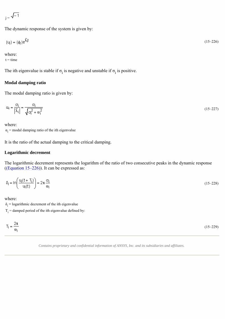
The dynamic response of the system is given by:

where:

The ith eigenvalue is stable if σi is negative and unstable if σi is positive.

Modal damping ratio

The modal damping ratio is given by:

where:

It is the ratio of the actual damping to the critical damping.

Logarithmic decrement

The logarithmic decrement represents the logarithm of the ratio of two consecutive peaks in the dynamic response ((Equation 15–226)). It can be expressed as:

where:

Contains proprietary and confidential information of ANSYS, Inc. and its subsidiaries and affiliates.

j =

(15–226)

t = time

(15–227)

αi = modal damping ratio of the ith eigenvalue

(15–228)

δi = logarithmic decrement of the ith eigenvalue

Ti = damped period of the ith eigenvalue defined by:

(15–229)