Embed Size (px)
Citation preview
The Institute for Food Economics and Consumption Studies
of the Christian-Albrechts-Universität Kiel
Climate-Smart Agriculture in Pakistan: Implications for Climate Risk Management,
Food Security, and Poverty Reduction
Dissertation
Submitted for Doctoral Degree
awarded by the Faculty of Agricultural and Nutritional Sciences
of the
Christian-Albrechts-Universität Kiel
Submitted by
Muhammad Faisal Shahzad (M.Sc.)
Born in Pakistan
Kiel, 2020


The institute for Food Economics and Consumption Studies
of the Christian-Albrechts-Universität Kiel
Climate-Smart Agriculture in Pakistan: Implications for Climate Risk Management,
Food Security, and Poverty Reduction
Dissertation
Submitted for Doctoral Degree
awarded by the Faculty of Agricultural and Nutritional Sciences
of the
Christian-Albrechts-Universität Kiel
Submitted by
Muhammad Faisal Shahzad (M.Sc.)
Born in Pakistan
Kiel, 2020
Examination Board:
Chairman: Prof. Dr. Dr. Christian Henning (Dean)
Examiner: Prof. Dr. Awudu Abdulai
Examiner: Prof. Dr. Martin Schellhorn
Assessor: Prof. Dr. Marie Catherine Riekhof
Date of Oral Examination: 17. 06. 2020.


v
Gedrukt mit der Genehmingung der Agrar-und Ernärungswissenschftlichen Facultät der
Christian-Albrechts Universität zu Kiel.
Diese Arbeit kann als pdf-Dokument unter https://macau.uni-kiel.de/receive/macau_mods_0000
0648 dem Internet geladen werden.

vi
Dedication
I dedicate this dissertation to my father Haji Farzand Ali, my mother Shamim Akhter, and the
whole family. I hope that this achievement will complete the dream that you had for me all those
many years ago when you chose to give me the best education you could. I further dedicate this
work to future generations of researchers entering the field of climate change impact assessment
and nutritional sciences. May you find a world worthy of your passion, dedication, and talent. If
you don’t, help us build it.

vii
Acknowledgments
First of all, I am thankful to Almighty Allah (SWT), the sustainer of the Universe, for giving me
the strength, good health, and wisdom to complete this milestone successfully. I am thankful to
beloved Prophet Hazrat Muhammat (PBUH) for his eminent aphorisms and encouragement about
knowledge acquisition that give me full strength to accomplish this program. I want to give thanks
to all the persons that have become a big part of this research. To my family, especially to my
father, mother, wife, sisters, and brothers for their moral support and prayers in order to complete
this study. I am obliged to present my utmost gratitude to my doctoral mentor, a great thinker and
generous soul, Prof. Dr. Awudu Abdulai, for guiding and helping me in order to make the study a
well-done achievement. His inspiring questions during lab group meetings, the stimulating and
engaging discussion has given me the impetus to go further during the memorable hours that I
have spent at my computer writing and revising research papers. I further extend the gratitude to
all dearests who live in my heart and colleagues, especially at the Institute of Food Economics and
Consumption Studies, who helped me to do this study presentable. With gratitude, my special
thanks also go to the Higher Education Commission (HEC) of Pakistan, and the German Academic
Exchange Service (DAAD) for the financial support granted to me throughout the study period. I
am also thankful to Haji Muhammad Hussain (lately deceased) and Manzoor Hussain Lehri for
their personal guarantee after securing HEC scholarship. A bundle of thanks to Dr. Muhammad
Shakir Aziz and Dr. Asif Naeem for proofreading this document. I am also thankful to the data
collection team for their quality work during the field survey. Finally, thanks to all the respondents
for their full cooperation that made them a big part of this study.
Kiel, June 2020. Muhammad Faisal Shahzad
Email: [email protected]

viii

ix
Table of Contents
List of Tables .............................................................................................................................. xiii
List of figures .............................................................................................................................. xv
Abstract ...................................................................................................................................... xvi
Zusammenfassung ................................................................................................................... xviii
Chapter 1
General Introduction ................................................................................................................... 1
1.1. Background ......................................................................................................................... 1
1.2. Problem setting and motivation ........................................................................................... 3
1.3. Climate and geography of Pakistan ..................................................................................... 9
1.4. Review of Pakistan’s agricultural sector and climate change impacts .............................. 12
1.5. Brief profile of Punjab province (study area) .................................................................... 14
1.6. Study objectives ................................................................................................................ 17
Future outlook of the study ...................................................................................................... 17
Structure of the dissertation ...................................................................................................... 18
References ................................................................................................................................ 20
Chapter 2
Adaptation to Extreme Weather Conditions and Farm Performance in Rural Pakistan ... 27
Abstract .................................................................................................................................... 27
2.1. Introduction ....................................................................................................................... 28
2.2. Materials and methods ...................................................................................................... 32
2.2.1. Modeling adaptation to extreme weather conditions ................................................. 32

x
2.2.2. Selection into adaptation to extreme weather conditions ........................................... 34
2.2.3. Impact assessment of adaptation to extreme weather conditions ............................... 34
2.2.4. Estimation and identification ..................................................................................... 36
2.2.5. The empirical specification ........................................................................................ 39
2.2.6. Study area ................................................................................................................... 42
2.2.7. Data collection and data description .......................................................................... 44
2.3. Empirical Results .............................................................................................................. 46
2.3.1. Descriptive statistics and mean differences between adopters and non-adopters. ..... 46
2.3.2. Determinants of adaptation to extreme weather conditions ....................................... 50
2.3.3. Volatility of farm net returns ...................................................................................... 51
2.3.4. Downside risk exposure and kurtosis ......................................................................... 53
2.3.5. Farm net returns ......................................................................................................... 56
2.3.6. Average treatment effects on the treated (ATT) ......................................................... 59
2.4. Discussion ......................................................................................................................... 59
2.5. Conclusion and policy implications .................................................................................. 62
Acknowledgments .................................................................................................................... 63
References ................................................................................................................................ 64
Appendix A .............................................................................................................................. 72
Chapter 3
Climate Risk Management in Agricultural and Rural Household Welfare: Empirical
Evidence from Pakistan ............................................................................................................. 78
Abstract .................................................................................................................................... 78

xi
3.1. Introduction ....................................................................................................................... 79
3.2. Data and descriptive statistics ........................................................................................... 83
3.3. Methodology ..................................................................................................................... 89
3.3.1. Conceptual framework ............................................................................................... 89
3.3.2. Empirical Strategy ...................................................................................................... 91
3.3.3. Counterfactual analysis and average treatment effects on the treated (ATT) ............. 97
3.4. Results and discussion ....................................................................................................... 98
3.4.1. Determinants of climate-smart farm practices ........................................................... 98
3.4.2. Economic implications of climate-smart agricultural practices ............................... 101
3.5. Conclusion and policy implications ................................................................................ 109
References .............................................................................................................................. 112
Appendix B ............................................................................................................................ 119
Chapter 4
The Heterogeneous Effects of Adoption of Climate-Smart Agriculture on Household
Welfare in Pakistan .................................................................................................................. 125
Abstract .................................................................................................................................. 125
4.1. Introduction ..................................................................................................................... 126
4.2. Conceptual framework and estimation ............................................................................ 129
4.3. Study area, data collection and data description ............................................................. 134
4.3.1. Study area ................................................................................................................. 134
4.3.2. Data collection and data description ........................................................................ 134
4.4. Results and discussion ..................................................................................................... 140

xii
4.4.1. First stage (selection equation) results ..................................................................... 141
4.4.2. Second stage estimation ........................................................................................... 144
4.4.3. Marginal treatment effects (MTE) results ................................................................ 151
4.4.4. Robustness checks .................................................................................................... 155
4.4.5. Summary of causal effects of adoption on food security and poverty ..................... 157
4.4.6. Simulating policy strategies ..................................................................................... 159
4.5. Conclusion and policy implications ................................................................................ 161
References .............................................................................................................................. 164
Appendix C ............................................................................................................................ 170
Chapter 5
Conclusion and policy implications ........................................................................................ 172
5.1. Summary of empirical methods ...................................................................................... 174
5.2. Summary of results .......................................................................................................... 176
5.3. Policy implications .......................................................................................................... 179
Appendix 1: Questionnaire ...................................................................................................... 181

xiii
List of Tables
Table 1.1 Climate, soil types and crops of agro-ecological zones in Pakistan ............................. 11
Table 1.2 Agriculture and socio-economic indicators of Pakistan ............................................... 13
Table 1.3 Climate and characteristics of agro-ecological zones of Punjab province ................... 16
Table 2.1 Definition and descriptive statistics of selected variables…………………………… 47
Table 2.2 Descriptive statistics and mean difference between adopters and non-adopters .......... 48
Table 2.3 Determinants of adaptation to extreme weather conditions and its impact on the
volatility of farm net returns. ........................................................................................................ 52
Table 2.4 Determinants of adaptation to extreme weather conditions and its impact on downside
risk exposure. ............................................................................................................................... 54
Table 2.5 Determinants of adaptation to extreme weather conditions and its impact on Kurtosis.
...................................................................................................................................................... 55
Table 2.6 Determinants of adaptation to extreme weather conditions and its impact on household
farm net returns ............................................................................................................................ 57
Table 2.7 Impact of adaptation to extreme weather conditions on farm net returns, the volatility
of farm net returns, and downside risk exposure.......................................................................... 59
Table 2.A1 Log-linear farm net returns function estimation…………………………………… 73
Table 2.A2 Residuals calculation of potential endogenous variables .......................................... 74
Table 2.A3 Instrumental variables validation test (Probit model) ................................................ 75
Table 2.A4 Instrumental variables validation test non-adopters (OLS) ....................................... 76
Table 2.A5 Instrumental variable correlation test ........................................................................ 76
Table 3.1 Definition and descriptive statistics of selected variables…………………………… 86
Table 3.2 Summary statistics of the variables used for the CSA adopters and non-adopters ...... 88
Table 3.3 Determinants of CSA practices choices, MNL model estimation .............................. 100
Table 3.4 Impact of CSA practices choices on farm net returns, second stage MESR estimation
.................................................................................................................................................... 103

xiv
Table 3.5 Overall average treatment effects on the treated ........................................................ 105
Table 3.6 Location-wise average treatment effects on the treated ............................................. 106
Table 3.7 Quantile-wise average treatment effects on the treated .............................................. 108
Table 3.B1 Impact of CSA practices on risk exposure, second stage MESR estimation …….. 119
Table 3.B2 Test on the validity of selection and potential endogenous variable instruments (Farm
net returns) .................................................................................................................................. 120
Table 3.B3 Test on the validity of selection and potential endogenous variable instruments
(Skewness) ................................................................................................................................. 120
Table 3.B4 Parameters estimates of net returns function ........................................................... 121
Table 3.B5 Parameter estimates of potential endogenous variable credit constraint ................. 122
Table 3.B6 Parameter estimates of of potential endogenous variable extension services ......... 123
Table 3.B7 Suest-based Hausman tests of IIA assumption ........................................................ 123
Table 3.B8 Correlation matrix .................................................................................................... 124
Table 3.B9 Robustness checks ................................................................................................... 124
Table 4.1 Descriptive Statistics and definition of selected variables…………………………. 139
Table 4.2 Descriptive statistics and mean difference between adopters and non-adopters ........ 140
Table 4.3 Selection equation and outcome equations results for HFIAS ................................... 146
Table 4.4 Selection equation and outcome equations results for HDDS .................................... 148
Table 4.5 Selection equation and outcome equations results for poverty headcount ................. 150
Table 4.6 Selection equation and outcome equations results for poverty gap (severity) ........... 151
Table 4.8 Impact of different policies on propensity scores and outcome variables .................. 160
Table 4.C1 Test on the validity of the selection instruments HFIAS…………………………. 170
Table 4.C2 Test on the validity of the selection instruments HDDS .......................................... 170
Table 4.C3 Test on the validity of the selection instruments poverty headcount index ............. 171
Table 4.C4 Test on the validity of the selection instruments poverty gap index ........................ 171
Table 4.C5 Matrix of correlations .............................................................................................. 171
xv
List of figures
Fig. 1.1 Schematic diagram showing the impacts of climate change on water, agriculture, food
security, and household welfare ..................................................................................................... 8
Fig. 1.2 Division of agro-ecological zones of Pakistan ................................................................ 10
Fig. 1.3 Map of Punjab province divided into agro-ecological zones .......................................... 15
Fig. 2.1 Map of Pakistan showing study area and agro-ecological zones…………………….... 43
Fig. 2.A1 Kernel density plot for adopters and non-adopters (Net Returns)…………...……… 77
Fig. 3.1 Map of Pakistan showing study area and data collection sites .………………………. 85
Fig. 3.2 Unconditional farm net returns distributions by CSA practices ..................................... 87
Fig. 4.1 Map of Pakistan showing study area and data collection sites………………………. 135
Fig. 4.2 Common support ........................................................................................................... 142
Fig. 4.3 MTE curve for household food insecurity access scale (HFIAS) ................................. 153
Fig. 4.4 MTE curve for household dietary diversity scores (HDDS) ........................................ 153
Fig. 4.5 MTE curve for poverty headcount index ...................................................................... 154
Fig. 4.6 MTE curve for poverty severity .................................................................................... 154
Fig. 4.7 MTE curves for HFIAS: functional form robustness checks ........................................ 155
Fig. 4.8 MTE curves for HDDS: functional form robustness checks ........................................ 156
Fig. 4.9 MTE curves for poverty headcount: functional form robustness checks ..................... 156
Fig. 4.10 MTE curves for poverty gap: functional form robustness checks .............................. 157

xvi
Abstract
Climate-smart agriculture (CSA) has emerged as a framework for developing and implementing
robust agricultural systems, which simultaneously improve food security, living conditions in
rural areas, facilitate adaptation to climate change, provide mitigation benefits and improve
household welfare. In recent decades, climate variability has made the world agricultural systems
more uncertain, causing reproductive failure and severe yield reductions in many crops. At the
same time, a growing population with increasing food demand and poverty appeal to adopt CSA
at the household level. As adoption rates in developing countries like Pakistan are low, the adverse
impacts of climate change such as temperature increases, erratic rainfall patterns, extreme weather
conditions significantly undermine agricultural production and food systems in such countries,
where hunger, malnutrition, and poverty are already predominant. Climate-smart agricultural
(CSA) practices appear to be useful tools in the form of adaption strategies to manage agricultural
farms that reduce climate risks and increase farm productivity in the developing world. This study,
therefore, contributes to the growing literature on the impact of CSA practices on farm
performance, and rural household welfare by exploring climate risk management, the contribution
of single or joint adaptation strategies in enhancing farm net returns, food and nutrition security,
as well as poverty reduction in rural Pakistan. In particular, the study first examines adaptation to
extreme weather conditions impact on farm net returns, and risk measures of this outcome variable
(volatility, downside risk exposure, and kurtosis) by using endogenous switching regression
(ESR) model to account for selection bias. Secondly, the study employs multinomial endogenous
switching regression (MESR) to explore climate risk management through multiple adaptation
practices and their impact on household welfare. The study also inspects factors influencing
farmers’ decisions to adopt these practices. Finally, the marginal treatment effect approach is
employed in analyzing the food and nutrition security as well as the poverty status of rural farm
households. The empirical results reveal that adoption of CSA practices exerts a positive and
significant impact on reducing volatility, downside risk exposure, and kurtosis of farm net returns.

xvii
The results further reveal that farmers who adopted CSA practices obtain higher farm net returns.
The collective findings from the study show that farmers’ decisions to adopt CSA practices are
mainly influenced by temperature and rainfall shocks, education of household head, extension
services, the experience of past climate-related shocks (such as floods, droughts, and pest
infestation, etc.), climate change information, climate change perception and climate-resilient
trainings. Credit constraint is the major barrier faced by the farmers in adopting CSA practices,
causing low adoption rates. In the multiple CSA practices’ adoption analysis, the results reveal
that soil and water conservation coupled with crop rotation as soil and water conservation exerts
the maximum impact on farm net returns earned from adapted plots followed by input mix,
diversifying seed variety, and changing cropping calendar, respectively. The findings also show
that all of the CSA practices significantly reduce downside risk exposure and crop failure of farm
households. Besides, controlling household and farm-level characteristics, climate variability, and
regional dummies, the empirical results confirm that observable and unobservable heterogeneity
significantly varies across farm households. The results further reveal that adoption of CSA
practices significantly reduces household food insecurity and increases household dietary
diversity at the lower level of unobserved resistance to adoption and vice versa. The findings also
show that farmers who adopted CSA practices experience a lower level of poverty than traditional
farmers. These findings call for development policy measures to promote CSA practices across
the country through climate change awareness, climate-resilient trainings, and access to extension
as well as formal and informal credit sources to enhance adoption rates for increasing agricultural
productivity and expanding food systems for a growing population.
Keywords: Climate-smart agriculture, climate change, impact assessment, risk management, food
security, poverty reduction, household welfare, Pakistan.

xviii
Zusammenfassung
Die Entwicklung und Implementierung von robusten Landwirtschaftssystemen, die darauf
abzielen Ernährungssicherheit, rurale Lebensbedingungen und Haushaltswohlfahrt zu verbessern,
zeitgleich den Klimawandel abzuschwächen und die Anpassung an diesen zu erleichtern, wird
unter dem Rahmenbegriff climate-smarte Landwirtschaft (CSA) zusammengefasst. Innerhalb der
letzten Jahrzehnte, haben Klimaschwankungen weltweit zu Unsicherheiten in der
landwirtschaftlichen Produktion geführt, die bei diversen Feldfrüchten Unfruchtbarkeit und
Ernteausfälle zur Folge hatten. Gleichzeitig stellt die wachsende Bevölkerung mit ihrer
gesteigerten Nachfrage nach Lebensmitteln, sowie zunehmende Armut einen Anreiz dar, CSA
vermehrt auf Haushaltsebene anzuwenden. Vor allem Entwicklungsländer wie Pakistan, wo
Hunger, Unterernährung und Armut bereits vorherrschend sind, sind stark von den Auswirkungen
des Klimawandels betroffen. Steigende Temperaturen, unregelmäßige Niederschläge und eine
Zunahme an extremen Wetterereignissen schwächen die landwirtschaftliche Produktion in diesen
Ländern signifikant, während CSA wenig verbreitet ist. Climate-smarte Landwirtschaftliche
(CSA) Praktiken erscheinen als nützliche Strategien zur Adaption, um vom Klimawandel
verursachte Risiken zu senken (Climate Risk Management) und die landwirtschaftliche
Produktivität in diesen Ländern zu steigern. Diese Arbeit analysiert Climate Risk Management,
die Auswirkung von einzelnen oder mehreren Adaptionsstrategien auf Netto-Betriebserträge,
Ernährungssicherheit, sowie Armutsreduzierung im ländlichen Pakistan und leistet somit einen
wichtigen Beitrag zur wachsenden Literatur über die Auswirkungen von CSA Praktiken auf die
Landwirtschaft und ländliche Haushaltswohlfahrt. Im Speziellen, untersucht die Arbeit zuerst, wie
sich eine Anpassung an Extremwetterereignisse auf die Netto-Betriebserträge und dessen
Risikomaße (Volatilität, Downside Risk Exposition und Kurtosis) auswirkt. Dabei wird das
endogenous switching regression (ESR) Modell angewandt, um Selektionseffekte zu
berücksichtigen. Zweitens, wird Climate Risk Management in Form von multiplen
Adaptionsstrategien und dessen Auswirkung auf Haushaltswohlfahrt mit Hilfe der multinomial

xix
endogenous switching regression (MESR) Methode analysiert. Diese Studie prüft zudem, welche
Faktoren Landwirte dazu bewegen, Adaptionsstrategien umzusetzen. Schließlich wird der Ansatz
des marginal treatment effect angewandt, um Ernährungssicherheit und Armut in ländlichen
Farmhaushalten zu untersuchen. Die empirischen Ergebnisse zeigen einen positiven und
signifikanten Einfluss von CSA Praktiken auf die Reduzierung von Volatilität, Downside Risk
Exposition und Kurtosis der Netto-Betriebserträge. Außerdem erzielen Landwirte, die CSA
Praktiken anwenden, höhere Netto-Betriebserträge. Die Entscheidung eines Landwirts CSA
Praktiken einzuführen, wird von Niederschlags- und Temperaturschocks, Bildungsgrad des
Haushaltsvorstands, landwirtschaftlichen Beratungsdiensten und Trainingsprogrammen, die
Erfahrung vergangener Klimaschocks (wie Überschwemmungen, Dürren, Krankheitsbefälle, etc.),
sowie Informationen über und die Wahrnehmung vom Klimawandel signifikant beeinflusst. Die
größte Hürde der Landwirte, um CSA Praktiken umsetzen zu können, ist die Kreditrestriktion,
welche in geringen Adoptionsraten resultiert. Der Vergleich verschiedener CSA Praktiken ergab,
dass die Kombination von Boden- und Wasserschutz mit Fruchtwechsel den größten Einfluss auf
den Netto-Betriebsertrag aufzeigt, gefolgt von Input-Mischung, Diversifizierung von angebauten
Feldfrüchten und geänderte Fruchtfolge. Die Ergebnisse zeigen zudem, dass alle CSA Praktiken
signifikant die Downside Risk Exposition und Ernteausfälle reduzieren. Außerdem, bei
Berücksichtigung von Farm- und Haushaltsmerkmalen, Klimavariabilität und Standort, bestätigen
die empirischen Ergebnisse, dass beobachtbare und unbeobachtbare Heterogenität signifikant
zwischen Haushalten variiert. Weitere Ergebnisse zeigen, dass die Umsetzung von CSA Praktiken
bei geringerem unbeobachtaren Widerstand gegenüber einer Adoption die Ernährungssicherheit
und tägliche Ernährungsvielfalt signifikant erhöht. Zudem erfahren Landwirte, die CSA Praktiken
anwenden, geringe Armut als traditionelle Landwirte. All diese Ergebnisse unterstützen die
Forderung, CSA Praktiken als Entwicklungsmaßnahme in ganz Pakistan voranzutreiben. Mit
einem gesteigerten Bewusstsein hinsichtlich des Klimawandels, entsprechenden
Trainingsprogrammen und Zugang zu Beratungsdiensten, sowie zu formellen und informellen

xx
Kreditgebern kann die Adoptionsrate von CSA Praktiken erhöht, die landwirtschaftliche
Produktivität gesteigert und somit das Ernährungssystem auf die wachsende Bevölkerung
angepasst werden.
1
Chapter 1
General Introduction
1.1. Background
Severe climate change is making the world weather uncertain and has a devastating direct effect
on agriculture (Foresight, 2011; Parry et al., 2004; Shannon and Motha, 2015). The average global
increase in temperature has risen about 2-degree Fahrenheit (1 ℃) during the last decades and
probable to continue at a rapid rate (World Bank, 2013), while combined greenhouse gas emissions
from agriculture, forestry, and other land use account for 22% of global emissions (FAO, 2010).
As such, warm atmosphere, decrease in snowfall, rising sea level, unpredicted changes in
precipitation, and greenhouse gas emissions are causing extreme weather events (IPCC, 2013),
which as a consequence, adversely affects agriculture, food production and distribution, and rural
household welfare. Thus, these adverse extreme weather conditions affect the economic
performance of a country (Economic Survey of Pakistan, 2016).
Likewise, extreme climate conditions have a significant effect on soil moisture interaction, land
erosion, and earth’s temperature. Global warming is causing seasonal variations in crop sowing
and harvest patterns due to which production tends to decrease in the future. As a primary source
of income in developing countries, agriculture is still a significant contributor to the welfare and
socio-economic development (World Bank, 2008). In developing countries, small losses in
agriculture production cause greater loss of income because agriculture accounts for a more
significant share of GDP compared with an industrial country. Nevertheless, these abrupt and
extreme changes in weather conditions are adversely affecting agriculture crop yields
(Chmielewski and Muller, 2004; Sharma and Dobriyal, 2014).
Deterioration in agriculture productivity is causing persistent poverty in the farming community
and food insecurity as a whole. Yield losses of agriculture crops range between 5 to 25 percent,
which is alarming to feeding the enormously growing population (Schwarts and Randall, 2003).
The decrease in agricultural productivity results in several adversities, where food security and

2
poverty are the leading ones. Food security includes four major components: food availability;
food accessibility; food utilization; and food affordability (FAO, 2008). Unfortunately, climate
change has a considerable effect on all four dimensions (Vogel and Smith, 2002; Clover, 2003).
Climate-related food insecurity has a considerable direct and indirect effect on human health
(McMichael, et al., 2006). Declining food availability and accessibility are associated with
hazardous health problems, malnourishment, and stunt growth in children, serious health problems
in pregnancy for both mother and child. It also causes different diseases in children that undermine
child educational performance (UNICEF, 2014). In the future, the number of malnourished
children would become higher due to climate change (Nelson et al., 2010).
Furthermore, predictions indicate that variations in rainfall would drive 12 million people into
absolute poverty by damaging existing water resources. Mainly, monsoon variations cause a
disparity in water availability for irrigation. Projections indicate that North West areas of the south
Asian region are getting drier. The increase in temperature is leading dry regions towards droughts.
Pakistan is highly vulnerable and at high risk due to vague precipitation predictions. Loss of snow
cover results in river flow reductions, which are a reliable and stable source of irrigation. Due to
the rapid melting of snow water runoff in summers causes floods and creates considerable
reductions in dry season flow. Risks become severe if warming reaches 4℃ (IPCC, 2013; National
Climate Change Policy, 2011). However, it has been predicted that the local vulnerability of
climate change adverse impacts would remain persistent (Planning Commission of Pakistan,
2010).
From the above discussion, it can be concluded that the agriculture sector should overcome three
challenges i) sustainably increase agricultural production to meet global food demand, ii) adapt to
the impacts of climate change, iii) and reduce greenhouse gas emissions. The concept of climate-
smart agriculture (CSA) has been developed and promoted to overcome these challenges by FAO
(2010). CSA is an innovative approach projecting development pathway by buffering climate
change adverse effects so that agriculture sectors remain more productive and sustainable. CSA

3
builds resilience to climate risks, which is essential for rural households and communities to cope
with the uncertainty created by climate change and extreme weather conditions. Agricultural
production systems and food systems must endure substantial changes to achieve sustainability.
To buffer the adverse calamities and their impacts, CSA has emerged as a framework for
developing and implementing robust agricultural systems, which simultaneously improve food
security, living conditions in rural areas, facilitate adaptation to climate change, provide mitigation
benefits and improve household welfare (FAO, 2013). The global community has recommended
the incorporation of climate-smart farm practices (CSA practices) into national development plans
to mitigate the adverse impacts of climate change on agriculture (IPCC, 2007; World Bank, 2010).
Climate-smart farm practice is a practice on the farm, which sustainably increases agricultural
productivity, adapts and builds the resilience of agricultural and food systems to climate change,
and reduces greenhouse gas emissions from agriculture (FAO, 2013). The CSA practices such as
changing input mix and cropping calendar, crop diversification, diversifying seed variety, crop
rotation, soil and water conservation, using improved seed variety, income diversification, crop,
and livestock integration and improving irrigation efficiency are the strategies generally used to
reduce climate change adverse effects (Tubiello et al., 2008; Soglo and Nonvide, 2019).
1.2. Problem setting and motivation
Climate change and extreme weather conditions directly or indirectly affect agricultural
productivity and food production. Several studies have been addressed in recent decades on
adoption, climate change, food security and poverty, e.g., Hassan and Nhemachena, 2008; Di
Falco et al., 2011; Ali and Erenstein, 2017; Javed et al. 2014; Nelson et al., 2014; Issahaku and
Abdulai, 2020, etc. The study by Hassan and Nhemachena (2008) revealed that better access to
markets, extension and credit services, technology, and farm assets tend to increase the probability
of climate change adoption. They further investigated that mono-cropping is more vulnerable to
climate change in Africa. In drier areas, farmers would be benefited from increased rainfall. Di

4
Falco et al. (2011) conducted a study on climate change analysis by using endogenous switching
regression analysis. They analyzed farmers’ decision to adapt to climate change and the impact of
this adaptation on agricultural productivity. They found that access to extension services and credit
were the main drivers to climate change adaptation. They also found that adaptation increased
farm productivity. Javed et al. (2014) carried out a study on climate change impact on agriculture
in Pakistan. They used the fixed effect and instrumental variables for analyzing district-level panel
data. They concluded that an increase in temperature was harmful to agriculture. Their findings
revealed that agriculture production of the current year was dependent on previous year production.
Abid et al., 2016a and Di Falco and Veronesi (2014) explored climate risks, adaptation strategies,
and impact on household welfare. Abid et al. (2016a) conducted a study on climate change
vulnerability, adaptation, and risk perception at form level in Punjab Pakistan. They investigated
various climate-related risks perceived by farm households. Extreme temperature, insect attack,
animal diseases, and crop pests were the main climate-related risks to the farmers, while limited
water for irrigation, proper infrastructure availability and poverty were the other risks to the
farmers. Di Falco and Veronesi (2014) calculated environmental risk in the presence of climate
change considering the role of adaptation in the Nile Basin of Ethiopia. They found that past
climate adaptation reduced current downside risk exposure ensuring reduction in crop failure risk.
They also found that adaptation to climate change was a successful risk management strategy. It
was also concluded that adaptation to climate change for non-adopters was more beneficial in
reducing downside risk.
Several studies explored the climate change impacts on food security and poverty (McMichael et
al., 2006; Deressa et al., 2008; Patz et al., 2002, 2005; Kovats and Hajat, 2008; Azeem et al., 2016;
Ahmad et al., 2015; Iqbal and Arif, 2010). Climate change, extreme weather conditions, heat stress,
future food yields, and hunger are strengthening infectious diseases and pose considerable health
risks, McMichael et al. (2006) investigated studying climate change impacts. They found that
social, economic, and demographic disruptions discourse health risks. They suggested planned

5
preventive and adaptive strategies to cope with climate change adverse effects that were harmful
to human health. By using the vulnerability assessment approach, Deressa et al. (2008) found that
Afar and Somali regions were most vulnerable to climate change. They concluded that
vulnerability to climate change was extremely related to poverty (loss of adaptive capacity). They
recommended investment in irrigation techniques for the insurance of irrigation potential to
enhance agricultural production and food supply. They also suggested that early warning of
extreme weather events to the farmers as preventive measures.
Patz et al. (2005) explored that many human diseases were associated with climate variations.
Cardiovascular and respiratory diseases became dominant due to starvation from crop failure and
changed the way of disease transmission. Climate change's impact on human health remained
uncertain, as there was a lack of long-term data set, the extent of socio-economic variables, varied
immunity levels, and resistance to drugs. Projections revealed that health risks would increase due
to climate change, while Kovats and Hajat (2008) found that climate change would increase the
intensity and frequency of heatwaves that might increase heat-related mortality. Khan and Salman
(2012) investigated the relationship between human vulnerability index and climate-induced
disasters (floods). By employing logistic regression analysis, they indicated that ownership of
livestock, literacy rate, and access to electricity play a decisive role in the recovery of affected
households after floods. Patz and Kovats (2002) stated that climate change would suffer a low-
income population. Climate change impacts depend on access to health care, age, living region,
and public health care infrastructure. Energy consuming countries were responsible for global
warming while developing nations were at extreme risk.
However, the literature on the impact assessment of adoption of new emerging climate-smart
technologies, mainly on climate risk management, food, and nutrition security and poverty
reduction in Pakistani perspective, is scanty. Studies have shown that adaptation of adoption
strategies can minimize the adverse impacts of climate change. The study mentioned above by
Abid et al. (2016a) explained the climate-related risk and perceptions in graphical form, and some

6
studies just rely on studying wheat crops for food security in the country (Ahmed et al., 2014;
Abid et al., 2016b). Azeem et al. (2016) conducted a study on household vulnerability to food
insecurity in Punjab Pakistan by using a multilevel model. They found that the share of a
household that was at the risk of becoming food insecure was higher than the share of current
food-insecure households. People were not vulnerable due to poor resource endowments but due
to household level idiosyncratic risk. Abid et al. (2016b) conducted a study on climate change
adaptation and the impact on food security by using propensity score matching technique (PSM).
They considered wheat productivity and crop income as food security indicators. They found that
farmers used changing planting dates, crop varieties, and different fertilizer types as adaptation
strategies to cope with climate change adverse impacts. Furthermore, they confirmed that
education, farming experience, weather forecasting, access to agriculture extension, and
marketing information had a significant effect on the adaptation decision of farmers. They also
found that adaptation to climate change increased wheat productivity and crop income enhancing
farmer’s welfare and food security.
Ahmad et al. (2015) compiled their results studying farm household’s adaptation to climate change
on food security, taking into account different agro-ecologies of Pakistan. They employed the
potential outcome treatment effects model for analysis. Adaptation strategies were grouped into
four categories. Results from the study showed that climate change adapters were more food
secure than non-adopters. They further concluded that the education of male and female heads,
the structure of the house, crop diversification, livestock ownership, and non-farm income
improved food security significantly. Age of household head, small land holding, and food
expenditure management were negatively associated with food security. They constructed a food
security index by using principal component analysis. Iqbal and Arif (2010) found that land and
water resources were the base for food security. These resources were limited and prone to climate
change. They further clarified that studies projected that crop yield losses due to climate change

7
would increase, growing season length would decrease, water requirements would increase while
water availability would decrease in the future.
Above mentioned studies incorporated graphical analysis, logit model, propensity score matching
technique, and Heckman treatment effect model. As farmers’ decisions to adapt to innovative
technologies are based on their observable characteristics (education, farm size, soil fertility, etc.)
and unobservable characteristics (innate skills, risk preferences, motivation for adaptation, etc.),
such decisions are non-random. Therefore, without accounting for these observable and
unobservable characteristics, the results may be biased and inconsistent. The methodologies used
in most of the studies mentioned above do not account for selection bias. Some recent studies (Di
Falco et al. 2011; Abdulai and Huffman, 2014; Ma and Abdulai, 2016) used endogenous switching
regression to account for observable and unobservable characteristics, but their analysis was based
on a single crop. Most of the studies cited above used single crop such as wheat, rice, cotton, or
maize to conclude their results on farm income and household welfare. However, the conclusion
based on a single crop may under or overestimate the real impacts of adoption for several reasons.
For instance, if multi-product farmer applies soil and water conservation techniques for the wheat
crop, it might offer benefit to oilseed crops in the same season and increase the yield of cotton,
rice, maize, etc. in the following season, which may not be captured if a researcher considers only
wheat yield leaving out other crops. Furthermore, there might be a negative interaction between
crops in a mixed setting, where one crop may increase the yield of other crops (Tessema et al.,
2015). Additionally, Abdulai and Huffman (2014) analyzed the soil and water conservation
impacts on rice yield and net returns without accounting for climate variables. Moreover, the
inclusion of climate variables is quite crucial to account for plant growth and yield, and agriculture
as a whole (Ray et al., 2015).
For sustainable agriculture production and farm household development, information on climate
change impacts and potential adaptation strategies should be widely known to inform
environmentalists and policy-makers as well as farm households. The present study examines an

8
in-depth analysis and consequently provides information on the potential effects of climate change
on the welfare of farm households. The knowledge abstracted through this study would be
important to agricultural producers for production planning under innovative adaptation
technologies and their implementation at the micro-level. It would also serve as an important
source for policymakers, environmentalists, and agriculture scientists for effective decision
making and policy planning on different innovative technologies and their impact on agricultural
production. It would also be helpful for government and research institutes for budget allocation,
environment development programs, and development of new crop variety genotypes.
Fig. 1.1 illustrates a brief overview of climate change impacts on water resources, agriculture,
food security, and household welfare.
Fig. 1.1 Schematic diagram showing the impacts of climate change on water, agriculture,
food security, and household welfare

9
For the future sustenance of an increasing population, we need adequate research, policy, and
planning to feed an enormously growing population. As mentioned above, very few and limited
studies have been carried out on climate change, and food security in Pakistan. Therefore, a
comprehensive study on farm net returns and the climate situation in the country is widely needed
(Abid et al., 2016a). Consequently, this study intends to make a healthy endeavor in analyzing the
climate change effects on household welfare, investigate the influence of adaptation strategies on
climate risk management, farm net returns, food security, and poverty. In addition to the country-
specific contribution to literature, this study also extends the mixed cropping analysis by moving
away from mono-cropping analysis to mixed-cropping that exploits the interlink benefits from
multiple adaptation strategies. Also, limited studies have examined the adoption impacts of
multiple adaptation strategies on farmers’ productivity and exposure to risk, though from a mono-
cropping perspective (Di Falco and Veronesi, 2013; Iqbal et al., 2015). We incorporate multiple
adaptation strategies with multi-crops in our analysis.
The focus of this study is on the key factors influencing climate-smart adaptation strategies, as
well as the impact of these adaptation strategies on farm household welfare, including food,
nutrition security, and poverty in South Asian countries, using Pakistan as a case study. After
addressing some conceptual issues, this study makes a healthy attempt in building the link between
climate change (extreme weather events), agricultural productivity, climate risk management,
food security and poverty, the role of climate-smart practices in mitigating the adverse impacts of
climate change and extreme weather conditions as well as reducing production risks of rural
households in Pakistan. A brief overview of climate and geography, climate change impacts, and
agriculture in Pakistan with an overview of the study area is given below.
1.3. Climate and geography of Pakistan
On the world map, Pakistan is situated between the longitudes of 61° to 75° east and the latitudes
of 24° and 37° north, spreading on a total area of 796096 square km. The country’s climate is
subtropical and semi-arid. The annual average rainfall ranges between 500-900 mm in the sub-

10
mountainous and northern plains, but it varies to 125 mm in extreme southern plains. Summer
monsoon causes 70% rainfall in July to September, while 30% rainfall occurs during winter.
Summers in Pakistan are sweltering (more than 40 °C), while in winter, the temperature is few
degrees above the freezing point. In mountainous areas, the temperature is always lower than the
other parts of the country (Khan, 2004). The climate of Pakistan is categorized by extreme
temperature variants. High altitudes are cold while the temperature in the Baluchistan plateau is
higher. In summers temperature reach great heights in some regions of the country. Northern
mountains covered with snow with relatively lower temperatures. In summer, melting snow
provides water for irrigation. A heavy rainy season supervene from June to September called
Monsoon (Khan et al., 2009). Pakistan has been divided into ten agroecological zones based on
climate, land use, physiography, and water availability (see Fig. 1.2). The brief introduction and
climatic conditions are listed in Table 1.1, which illustrates the division of agroecological zones
in Pakistan.
Fig. 1.2 Division of agro-ecological zones of Pakistan

11
Table 1.1 Climate, soil types and crops of agro-ecological zones in Pakistan
Source: FAO, 2006; Khan, 2004.
Zone ID
Zone name
Mean summer
temp
(°C)
Mean
winter
temp
(°C)
Mean monthly summer rainfall (mm)
Mean monthly winter rainfall (mm)
Soil and land use Crops
I Indus Delta 30-40 19-20 75 <5 Clayey and silty soils, parts of clayey soils are under cultivation.
Rice, sugarcane, cotton millet, maize, barley, rape and mustard, gram, fodder, pulses, and vegetable
II Southern Irrigated Plain 40-45 8-12 18-55 <1 Silty, sandy loam, calcareous loam and clayey Cotton, wheat, sugar cane, rice, wheat, gram, berseem, and sorghum
III-a Sandy Desert Zone-a 46-50 4-10 20-25 20-25 Sandy and loamy fine sand, land is used for grazing
Millet, wheat, rape and mustard, fodder, cotton, sugarcane, sorghum, rice, maize, and pulses
III-b Sandy Desert Zone-b 40-48 3-10 25-30 25-30 Sandy and loamy fine sand, land is used for grazing
Cotton, sugarcane, rice, wheat, and gram. maize, sorghum and millet, pulses and vegetable
IV-a Northern Irrigated Plain Zone-a
39.5-42 6.2 25-42 25-42 Sandy loam-clay loam, clay, calcareous, saline-sodic
Wheat, rice, sugarcane, oilseeds, millets, cotton, sugarcane, maize as well as citrus and mangoes
IV-b Northern Irrigated Plain Zone-b
43-44 5 20-32 20-32 Silty clays and clay loams Sugar cane, maize, tobacco, wheat, berseem, sugar beet, and orchards
V
Barani (Rainfed) Lands 38.5 4-7 7-17 30-50 Silt loams, calcareous loams Rice, sorghum, millet, maize, pulses, groundnut, sugarcane, wheat, gram, rapeseed, mustard and barley
VI Wet Mountains 35 0-4 20 10 Silt loam to silty clays, non-calcareous to slightly, calcareous, land is used for rain-fed agriculture.
Forest, wheat, apple, olives
VII Northern Dry Mountains 36-40 −2.5-9 10-20 25-75 Deep, clayey, calcareous, non-calcareous, most land is used for grazing
Wheat and maize are grown rain-fed, rice is irrigated in local areas; fruits grown in flank streams
VIII Western Dry Mountains 30-39 −3-7.7 30-95 63-95
Loamy, deep and strongly calcareous, mountains have shallow soil
Apples, peaches, plums, apricots, grapes, wheat and maize
IX Dry Western Plateau 33-40.5 3-15 36-37 2.4 Silt loams, deep and strongly calcareous, land use is mainly grazing
Melons, sorghum, fruits, vegetables, and wheat is grown where spring or “Kareze” water is available
X Sulaiman Piedmont 40-43 5.8-7.6 13 <1 Loams, calcareous, with narrow strips of salinity sodicity, torrent-watered cultivation is the main land use
Wheat, millets, gram, and rice.

12
There are four seasons in Pakistan: a cold and dry winter from December to February, spring
season from March to May, summer or Monsoon season from June to September, and retreating
monsoon period or autumn from October to November. Pakistan has two cropping seasons “Rabi
(winter) season and Kharif (summer) season.” Rabi season crops are sown in October-December
and harvested in March-April. Kharif season is slightly longer; it starts from February-March and
continues up to December. Water from Northern areas flows into the Indus basin with its five
tributaries named Chenab, Jhelum, Ravi, Sutlej, and Beas. Indus basin is the primary source of
irrigation for agriculture in Pakistan (Khan, 2004).
1.4. Review of Pakistan’s agricultural sector and climate change impacts
The agriculture sector is the backbone of Pakistan’s economy. It contributes 19.8 percent to
national GDP and employs 42.3 percent labor force of the country. Pakistan is ranked 5th in the
world with 212.2 million inhabitants and plays a vital role in ensuring food security for this
relatively huge growing population. In Asian countries, farm sizes are petite, approximately 89%
of rural households in Pakistan are below 5 Hectare and cultivate 55% of the total agricultural
area. Pakistan exports agro-based products to other countries and receive 80% of the country’s
total export earnings. In this way, Pakistan’s agriculture has earned much enticing in recent years
as a vast population is relying on agriculture for its livelihood. But the growth of the agriculture
sector is dependent on favorable weather conditions. A strong relationship exists between
agriculture and climate. Weather conditions like temperature, precipitation, and extreme events
affect the economic performance of the country. Climate change has a significant impact on
production, commodity prices, and economic growth. Climate change and food security are the
incipient challenges that Pakistan faces currently. These challenges shifted the policy focus from
a few years (Economic Survey of Pakistan, 2016).
In Pakistan, three major grain crops are grown. Wheat is the top leading food grain and accounts
for 10.3 percent to value-added in agriculture and 2.2 percent to national GDP. Rice is the second
major food grain crop; its share in value-added in agriculture is 3.1 percent and accounts for 0.7

13
percent in GDP. Maize is the third major enriched food grain adding 2.1 percent to value-added in
agriculture and 0.4 percent to GDP. Gram, Jawar, Bajra, and Barley are the other grain crops grown
in Pakistan. Timely rainfall at regular intervals and favorable weather conditions result in
increased production of these crops. Due to floods and excessive rains, rice yield was not so
impressive. Other grain crops declined their production due to unfavorable weather conditions
(Economic Survey of Pakistan, 2014). Studies have shown that adaptation to climate change
reduce the adverse impacts of unfavorable weather conditions and help to increase production and
farm income. Some agriculture and socio-economic indicators of Pakistan are given in Table 1.2.
Table 1.2 Agriculture and socio-economic indicators of Pakistan
Index Figure
GDP growth 5.5%
Agricultural growth 3.8% *
Agriculture value added (% of GDP) 23%
Arable land (% of total land) 40.3%
Agricultural land (% of total land) 47.8%
Agricultural irrigated land (% of total agricultural land) 50.5%
Population 212.2 million
Rural vs. urban population share 64% vs. 36%
Poverty headcount ratio at national poverty lines (% of population) 24.3% (2015)
Source: World bank indicator data 2016, * Economic Survey of Pakistan, 2018.
Climate change costs Pakistani Rupees 365 billion every year in the form of inadequate water
supply, pollution, land degradation, and deforestation (Economic Survey of Pakistan, 2014).
Besides, climate change has a direct negative impact on crop yields in Pakistan (Gill, 2016). Major
crop yields are reduced with climate change adverse impacts (Janjua et al., 2010). Pakistan is
below the wheat production potential; a 60% gap exists that should be narrowed down. The
irrigated area of crops has been increased, but water availability has decreased. Water
requirements have significant importance at different stages of growth; some stages are more
vulnerable to water shortage and result in substantial wheat yield losses (PARC, 2013). Climate

14
change affects the rice crop when it is in the flowering and milking stage (Ahmad et al., 2014).
Maize yield has a negative relationship with temperature; higher temperature tends to low maize
yield (Khaliq, 2008). Temperature also negatively affect arid zone crop production, but
precipitation has a positive impact on crop yield. The combined effect of both is negative for the
arid zone in Pakistan (Shakoor et al., 2011).
As mentioned above, the issue of food security has become inevitable to address because
agricultural output has decreased with adverse impacts of climate change. The population of
Pakistan is increasing enormously. This rapid growth of population renders economic stability and
development of Pakistan. According to the National Nutritional Survey, about 60 percent
population is food insecure, and 50 percent of women and children are underfed (Economic
Survey of Pakistan, 2014). Punjab is the largest producer still has a 23.6 percent food insecure
population (SDPI, 2009). Pakistan once an exporter of wheat is now in danger to fulfill the needs
of domestic requirements for sustaining the growing population. The population of Pakistan will
grow 227 million up to 2025. Out of 107 countries, Pakistan is miserably at the 76th number in
the Global Food Security Index. Population growth, limited land for agriculture, increasing water
stress, restricted agricultural technology, and varying consumption patterns are raising the threat
of dearth and food shortage. Food security is a complex issue for Pakistan to resolve as it has
many facets (Economic Survey of Pakistan, 2014).
1.5. Brief profile of Punjab province (study area)
Punjab province is located at 31.17° N and 72.70° E with and area of about 205, 344 km2. It is
the most populous province of Pakistan spread over 26% of the land area. It borders with
Balochistan, Islamabad Capital Territory, Khyber Pakhtunkhwa, Sindh, and Azad Jammu and
Kashmir. From the Indian side, it borders with Indian Punjab, Rajasthan, and Indian Occupied
Kashmir. Indus River is the longest river of Pakistan; it flows through Punjab with five tributaries
Jhelum, Ravi, Sutlej, Chenab, and Beas. Punjab stems from Persian words “Punj” means five and
“ab” means water, naming it the land of five rivers. Upper Indus plain is the most important part

15
that contributes to Pakistan’s agriculture sector. It is called the “Grain Basket of the Sub-continent”
that shares the highest proportion of agriculture to the country’s gross domestic product (GDP).
Climatically, Punjab province is located in arid to semi-arid region of the country, where the
temperature ranges from −2 °C to 45 °C usually but sometimes reach 50 °C in summer and −7 °C
in winter. The maximum average annual temperature ranges from 28-32 °C, while the minimum
average annual temperature varies between 15-19 °C. There is an increasing trend in temperature
over time that is estimated to be more than 0.5 °C. From the last five decades, rainfall shows an
increasing trend with an average annual change of 228 mm. Punjab is blessed with four eminent
seasons, spring, summer, autumn, and winter. There are fourteen agroecological zones in Punjab
province with varying characteristics (FAO, 2019). Fig. 1.3 shows different agro-ecological zones
of Punjab province, while Table 1.3 illustrates the essential characteristics and climatic conditions
of these zones.
Source: FAO, 2019.
Fig. 1.3 Map of Punjab province divided into agro-ecological zones

16
Table 1.3 Climate and characteristics of agro-ecological zones of Punjab province
Source: FAO, 2019.
Zone
ID
Zone name
Avg, rabi
max temp
(°C)
Avg, rabi
min temp
(°C)
Avg, kharif
max temp
(°C)
Avg, kharif
min temp
(°C)
Avg,
annual
rainfall
(mm)
ET (mm)
Soil type
I Cholistan desert 28.09 12.31 39.28 27.31 230 3.20 Mostly sandy
II Arid irrigated 29.20 12.45 40.41 27.59 234 3.10 Loam, sandy loam (9%)
III Cotton–sugarcane 28.67 12.40 39.93 27.49 243 2.93 Sandy loam, clay loam (10%), loam (35%)
IV Rod-i-Kohi 27.73 12.61 39.42 27.28 255 3.10 Mostly sandy loam
V Semi-desert irrigated 27.59 12.38 38.94 27.22 412 2.88 Loam, sandy loam (20%), clay loam (8%)
VI Mix cropping 27.38 12.99 39.47 27.30 460 2.62 Sandy loam (55%), loam (45%), clay (5%), loam
VII Cotton mix cropping 27.39 12.08 38.52 26.72 580 2.71 Loam, sandy loam (5%)
VIII Maize wheat mix cropping 26.97 11.06 37.86 25.58 590 2.64 Loam, sandy loam (3%), clay loam (1%)
IX Thal-Gram crop 27.51 11.35 39.21 26.24 612 2.25 Sandy loam (50%), sandy (35%), loam (10%), clay (5%)
X Rice–wheat 26.34 11.80 36.96 25.74 760 2.74 Loam, clay loam (5%), sandy loam (3%)
XI Thal zone 2 26.84 10.91 37.80 25.73 1 120 2.34 Sandy loam (45%), loam (45%), clay loam (5%)
XII Rice zone 25.03 11.71 35.53 25.20 1 250 1.76 Loam (40%), sandy loam (20%), clay loam (10%)
XIII Groundnut-medium rainfall 24.85 10.27 36.36 24.37 1 620 2.10 Loam (95%), sandy loam (5%)
XIV High rainfall 23.35 9.45 34.50 22.96 1 780 1.95 Loam (95%), sandy loam (5%)

17
Being the most populous, Punjab is the leading province for the agricultural production in Pakistan.
By covering 69% of the total cropped area, it contributes a significant share in the agricultural
economy of the country. Notably, the province accounts for 97% of rice, 83% of cotton, 63% of
sugarcane, and 51% of maize to the national crop production (FAO, 2019). Climate change poses
a formidable challenge to the farmers in the province and reduced major crop yields. This year
major crop growth rates are recorded negative, while the overall negative growth rate of 0.19% is
observed in the agriculture sector of the country (Economic Survey of Pakistan, 2019). Therefore,
climate risk management through adaptation may help to reduce the adverse impacts of climate
change and extreme weather conditions. A rigorous analysis of these adaptation strategies may
provide insights into which adaptation measures should be taken to cope with the adversities and
which of them single or a combination may be useful in enhancing crop yields and farm income
in the province.
1.6. Study objectives
The main objective of this research study is to assess the impact of climate-smart agriculture
adoption on farm performance in Pakistan. Specifically, the aims of this study are:
1- To assess environmental risks to agriculture under extreme weather conditions and their
management at the household level;
2- To determine the contributing factors to the household decision choices to adapt to different
climate-smart agricultural practices and their impact on household welfare;
3- To estimate the impact of adoption of climate-smart agricultural practices on food and nutrition
security and poverty reduction.
Future outlook of the study
This study analyses the climate change adoption impacts on agricultural production, climate risk
management in agriculture, food and nutrition security, and poverty reduction. However,
agriculture is mainly dependent on water resources available for irrigation in the country. In

18
Pakistan, most of the commercial farms have access to water. Notably, about 80% of the crop area
is irrigated, and 90% of the farm output comes from irrigated land. Besides, monsoon rainfall
plays a vital role in agricultural production in Pakistan. However, climate change is considerably
affecting water resources and glacier cover. Approximately 75 percent of Himalayan glaciers will
disappear from the surface of the earth by 2035 (Misra, 2014). These glaciers are the major and
stable source of water for irrigation in Pakistan (Bashir and Rasul, 2010). It is further predicted
that climate change has a considerable effect on water resources in the Indus Basin (Zhu et al.,
2013). Pakistan is classified as a water-stressed country that is rafting toward water scarcity if
adequate measures not taken (GOP, 2014; World Economic Forum, 2013). One leading cause of
the reduction in agricultural output is water shortage for irrigation in Pakistan (Abid et al., 2016a).
Further research on climate change impacts on water resources could be helpful in finding the
possible solutions to conserve water resources of the country to improving agriculture and food
production. As climate change tends to positively influence innovation processes through
information sources and training, therefore, one domain could be the impact of information
diffusion processes and cultural change on adoption of climate smart agriculture. Besides,
assessment of the impact of adoption of climate smart agricultural technologies on farm input
allocation and environmental efficiency could be another area of research.
Structure of the dissertation
This dissertation is a collection of research articles and organized as follows. The article in Chapter
2 explores the adoption of extreme weather conditions and farm performance in rural Pakistan.
Extreme weather conditions pose a formidable challenge to the farmers and increase production
risks to the community. To the extent that these risks vary across agro-ecological zones, and the
decision to adopt extreme weather conditions is non-random. Therefore, we employ endogenous
switching regression that accounts for observable and unobservable factors to ensure unbiased and
consistent estimates. Specifically, we analyze the factors affecting adoption decisions of extreme
weather conditions and the impact of adoption on farm net returns and the measures of risk
19
exposure such as variance, skewness, and kurtosis. Chapter 3 examines the adaptation implications
of CSA practices in terms of climate risk management and farm household welfare. Specifically,
chapter investigates the drivers of adoption of different CSA practices such as changing cropping
calendar, diversifying seed variety, changing input mix and soil and water conservation, and the
impact of adoption of these practices on farm net returns and downside risk exposure. In this
chapter, we employ multinomial endogenous switching regression to account for selection bias
and unobservable heterogeneity. Chapter 4 assesses the impacts of CSA practices on food and
nutrition security and poverty reduction. Specifically, we examine heterogeneity in CSA effects
on household welfare in Pakistan by employing marginal treatment effects approach. Chapter 5
presents the conclusion and policy implications of the study.

20
References
Abdulai, A., & Huffman, W., (2014). The adoption and impact of soil and water conservation
technology: An endogenous switching regression application. Land Economics, 90(1),
26-43.
Abid, M., Schilling, J., Scheffran, J., & Zulfiqar, F., (2016a). Climate change vulnerability,
adaptation and risk perceptions at farm level in Punjab, Pakistan. Science of the Total
Environment, 547, 447-460.
Abid, M., Schneider, U. A., & Scheffran, J. (2016b). Adaptation to Climate Change and Its
Impacts on Food Productivity and Crop Income: Perspectives of Farmers in Rural
Pakistan, Journal of Rural Studies, 47, Part A, 254-266.
Ahmad, M., Mustafa, G., & Iqbal, M. (2015). Impact of Farm Households’ Adaptations to Climate
Change on Food Security: Evidence from Different Agro-ecologies of Pakistan.
Ahmad, M., Nawaz M., Iqbal M., Javed, S. A. (2014). Analyzing the Impact of Climate Change
on Rice Productivity in Pakistan. PIDE climate Change Working Paper Series. Paper
No. 2: 2014.
Ali, A., & Erenstein, O. (2017). Assessing farmer use of climate change adaptation practices and
impacts on food security and poverty in Pakistan. Climate Risk Management, 16, 183-
194.
Azeem, M. M., Mugera, A. W., & Schilizzi, S. (2016). Living on the edge: Household
vulnerability to food-insecurity in the Punjab, Pakistan. Food Policy, 64, 1-13.
Bashir, F., & Rasul, G. (2010). Estimation of average snow cover over northern Pakistan. Pakistan
Journal of Meteorology, 7(13), 63-69.
Chmielewski, F. M., Muller, A., & Bruns, E. (2004). Climate changes and trends in phenology of
fruit trees and field crops in Germany, 1961–2000. Agricultural and Forest Meteorology,

21
121(1), 69-78.
Clover, J. (2003). Food security in sub-Saharan Africa. African Security Studies, 12(1), 5-15.
Deressa, T., Hassan, R. M., & Ringler, C. (2008). Measuring Ethiopian farmers' vulnerability to
climate change across regional states. Intl Food Policy Res Inst.
Di Falco, S., & Veronesi, M. (2013). How can African agriculture adapt to climate change? A
counterfactual analysis from Ethiopia. Land Economics, 89(4), 743-766.
Di Falco, S., & Veronesi, M. (2014). Managing environmental risk in presence of climate change:
the role of adaptation in the Nile Basin of Ethiopia. Environmental and Resource
Economics, 57(4), 553-577.
Di Falco, S., M. Veronesi, and M. Yesuf. (2011). Does Adaptation to Climate Change Provide
Food Security? A Micro-perspective from Ethiopia. American Journal of Agricultural
Economics 93 (3): 829–46.
Economic Survey of Pakistan. (2018). Economic Advisor’s Wing, Ministry of Finance,
Islamabad, Pakistan.
Economic Survey of Pakistan. (2019). Economic Advisor’s Wing, Ministry of Finance,
Islamabad, Pakistan.
Economic Survey of Pakistan. (2014). Economic Advisor’s Wing, Ministry of Finance,
Islamabad, Pakistan.
Economic Survey of Pakistan. (2016). Economic Advisor’s Wing, Ministry of Finance,
Islamabad, Pakistan.
FAO. (2008). An Introduction to the Basic Concepts of Food Security Food and Agriculture
Association of the United Nations (FAO, Rome).
FAO. (2013). Climate-Smart Agriculture Sourcebook. Food and Agriculture Organization,
Rome.

22
FAO. (2019). Climate-Smart Agriculture for Punjab, Pakistan. Food and Agricultural
Organization (FAO), DOI: 10.13140/RG.2.2.25544.78083
FAO. (2006). Country Pasture/Forage Resource Profiles. Food and Agriculture Association of the
United Nations (FAO, Rome).
FAO. (2010). “Climate-smart” agriculture: policies, practices and financing for food security,
adaptation and mitigation. Rome.
Foresight. (2011). The future of food and farming. Final Project Report. London, The Government
Office for Science.
Gill, H. A. (2016). Pakistan-adaptations measures to cope with the rising temperature, 1.5 degree
regime. The Nature News, environment, climate change and science. Available at
http://thenaturenews.com/2016/08/pakistan-adaptations-measures-to-cope-with-the-
rising-temperature-1-5-degree-regime/
GOP. (2014). Pakistan Vision 2025. Ministry of Planning and Development Government of
Pakistan, Islamabad. Government of Pakistan, Islamabad.
Hassan, R., & Nhemachena, C. (2008). Determinants of African farmers’ strategies for adapting
to climate change: Multinomial choice analysis. African Journal of Agricultural and
Resource Economics, 2(1), 83-104
IPCC (2007). Climate Change 2007: Fourth Assessment Report of the Intergovernmental Panel
on Climate Change, Cambridge University Press, Cambridge.
IPCC. (2013). Fifth Assessment Report on Climate Change. Intergovernmental Panel on Climate
Change, Cambridge University Press, Cambridge.
Iqbal, M. M., & Arif, M. (2010). Climate-change aspersions on food security of Pakistan. A
Journal of Science for Development, 15.
Iqbal, M., Ahmad, M., & Mustafa, G. (2015). Impact of Farm Households’ Adaptation on

23
Agricultural Productivity: Evidence from Different Agro-ecologies of Pakistan.
Issahaku, G., & Abdulai, A. (2020). Household welfare implications of sustainable land
management practices among smallholder farmers in Ghana. Land Use Policy, 94,
104502.
Janjua, P. Z., Samad, G. and Khan, N. U. (2010). Impact of Climate Change on Wheat Production:
A Case Study of Pakistan. The Pakistan Development Review 49(4): 799–822.
Javed, S. A., Ahmad, M., and Iqbal, M. (2014). Impact of Climate Change on Agriculture in
Pakistan: A District Level Analysis. Pakistan Institute of Development Economics,
Climate Change Working Papers No. 3.
Khaliq, T. (2008). Modeling the impact of climate change on maize (zea mays l.) Productivity in
the Punjab. A PhD thesis department of Agronomy, University of Agriculture
Faisalabad, Pakistan.
Khan, A. G. (2004). The characterization of the agro ecological context in which fangr (farm
animal genetic resources) are found.
Khan, A. G., Afzal, M., & Usmani, R. H. (2009). The characterization of the agro ecological
context in which FAnGR (Farm Animal Genetic Resources) are found.
Khan, F. A., & Salman, A. (2012). A simple human vulnerability index to climate change hazards
for Pakistan. International Journal of Disaster Risk Science, 3(3), 163-176.
Khan, S. (2019). Climate classification of Pakistan. International Journal of Economic and
Environmental Geology, 10(2), 60-71.
Kovats, R. S., & Hajat, S. (2008). Heat stress and public health: a critical review. Annu. Rev.
Public Health, 29, 41-55.
Ma, W., & Abdulai, A. (2016). Does cooperative membership improve household welfare?
Evidence from apple farmers in China. Food Policy, 58, 94-102.

24
McMichael, A. J., Woodruff, R. E., & Hales, S. (2006). Climate change and human health: present
and future risks. The Lancet, 367(9513), 859-869.
Misra, A. K. (2014). Climate change and challenges of water and food security. International
Journal of Sustainable Built Environment, 3(1), 153-165.
National Climate Change Policy. (2011). National Climate Change Policy, Ministry of
Environment, Government of Pakistan.
Nelson, G. C., Mensbrugghe, D., Ahammad, H., Blanc, E., Calvin, K., Hasegawa, T., ... & Lampe,
M. (2014). Agriculture and climate change in global scenarios: why don't the models
agree. Agricultural Economics, 45(1), 85-101.
Nelson, G. C., Rosegrant, M. W., Palazzo, A., Gray, I., Ingersoll, C., Robertson, R., Tokgoz, S.,
Zhu, T., Sulser, T. B., Ringler, C., Msangi, S. and Liangzhi You, L. (2010). Food
security, farming, and climate change to 2050: Scenarios, results, policy options (Vol.
172). Intl Food Policy Res Inst.
PARC. (2013). Wheat in Pakistan. Wheat Plant Sciences Division Pakistan Agricultural Research
Council Islamabad, Pakistan. A status paper.
Parry, M. L., Rosenzweig, C., Iglesias, A., Livermore, M., & Fischer, G. (2004). Effects of climate
change on global food production under SRES emissions and socio-economic
scenarios. Global Environmental Change,14(1), 53-67.
Patz, J. A., & Kovats, R. S. (2002). Hotspots in climate change and human health. British
Medical Journal, 325(7372), 1094.
Patz, J. A., Campbell-Lendrum, D., Holloway, T., & Foley, J. A. (2005). Impact of regional
climate change on human health. Nature, 438(7066), 310-317.
Planning Commission of Pakistan. (2010). Final Report of the Task Force on Climate Change.
Planning Commission of Pakistan, Government of Pakistan.

25
Ray, D.K., Gerber, J.S., MacDonald, G.K., West, P.C. (2015). Climate variation explains a third
of global crop yield variability. Nat. Commun. 6, 5989.
Schwartz, P., & Randall, D. (2003). An abrupt climate change scenario and its implications for
United States national security. California Institute of Technology Pasadena Ca Jet
Propulsion Lab.
SDPI. (2009). Food insecurity in Pakistan. Sustainable Development Policy Institute, Islamabad.
Retrieved on 17 Oct 2016. Available at.
Shakoor, U., Saboor, A., Ali, I., Mohsin, A. Q. (2011). Impact of Climate Change on Agriculture:
Evidence from Arid Region. Pak. J. Agri. Sci. 48(4), 327-333
Shannon, H. D., & Motha, R. P. (2015). Managing weather and climate risks to agriculture in
North America, Central America and the Caribbean. Weather and Climate Extremes, 10,
50-56.
Sharma, P., & Dobriyal, P. (2014). Climate Change and Agricultural Sector in Uttarakhand.
Journal of Studies in Dynamics and Change, 1(1), 6-14.
Soglo, Y.Y., Nonvide, G.M.A. (2019). Climate change perceptions and responsive strategies in
Benin: the case of maize farmers. Climatic Change 155, 245–256.
Tessema, Y., Asafu-Adjaye, J., Rodriguez, D., Mallawaarachchi, T., & Shiferaw, B. (2015). A
bio-economic analysis of the benefits of conservation agriculture: The case of
smallholder farmers in Adami Tulu district, Ethiopia. Ecological Economics, 120, 164-
174.
Tubiello, F., Schmidhuber, J., Howden, M., Neofotis, P. G., Park, S., Fernandes, E., & Thapa, D.
(2008). Climate change response strategies for agriculture: challenges and opportunities
for the 21st century. Agriculture and rural development discussion paper, 42.
UNICEF. (2014). United Nations Children Fund. Pakistan Annual report 2013.
26
Vogel, C., & Smith, J. (2002). The politics of scarcity: conceptualising the current food security
crisis in southern Africa: commentary. South African journal of science, 98(7), 315-317.
World Bank. (2008). World Development Report 2008. Agriculture for Development. World
Bank Washington D.C.
World Bank. (2010). Economics of adaptation to climate change - Synthesis report (English).
Washington, DC: World Bank.
World Bank. (2013). World Development Report, 2013. Development and Climate Change.
World Bank Washington, D.C.
World Bank. (2016). World indicator data. World Bank Washington D.C.
World Economic Forum. (2013). The Global Risks report 2013, World Economic Forum, New
York, USA.
Zhu, T., Ringler, C., Iqbal, M. M., Sulser, T. B., and Goheer, M. A. (2013). Climate change
impacts and adaptation options for water and food in Pakistan: scenario analysis using
an integrated global water and food projections model. Water International 38(5), 651-
669.

27
Chapter 2
Adaptation to Extreme Weather Conditions and Farm Performance in Rural Pakistan
Muhammad Faisal Shahzad and Awudu Abdulai
Department of Food Economics and Consumption Studies
Published in Agricultural Systems (Volume 180, 2020).
Abstract
Extreme weather conditions resulting from climate change pose a formidable challenge to many
farmers worldwide. In this article, we analyze farmers’ adaptation to extreme weather conditions
using climate-smart farm practices (CSA practices), and the impact of adoption of these adaptation
strategies on farm performance, using recent farm-level data from three agro-ecological zones of
Pakistan. Most of the earlier studies on Pakistan used methods that did not account for unobserved
characteristics such as innate skills and risk preferences, resulting in inconsistent estimates. We
employ an endogenous switching regression model to account for potential endogeneity and
selection bias arising from observable and unobservable factors. The empirical results show that
adoption of CSA practices contributes to higher farm net returns. The findings further reveal that
adoption of these practices significantly reduces volatility of farm net returns and farmers’
exposure to downside risk. We also find that access to extension services and education of the
household head positively influence the likelihood of adapting CSA practices in response to
extreme weather conditions.
Keywords
Extreme weather conditions, climate-smart practices, impact assessment, farm performance,
Pakistan.

28
2.1. Introduction
Adoption of climate-smart farm practices (CSA practices) that can mitigate extreme weather
conditions in the face of climate change can improve farm performance and household welfare in
developing countries, particularly through adopting new technologies against climate change.
Many previous studies have highlighted the significant effects of climate change on profits, farm
income, and farm productivity (e.g., Deschenes and Greenstone, 2007; Nhemachena et al., 2014;
Huang et al., 2015). However, very few studies have investigated how adaptation to extreme
weather conditions influence risk exposure of climate susceptible farmers and household welfare
(e.g., Bouwer, 2019; Vasileiadou et al., 2014; IPCC, 2012). Some studies have shown that climate
change adversely affects agriculture in Pakistan, while adaptation to climate change has had a
shielding effect (Abid et al., 2016a; Ali and Erenstein, 2017). The adaptation strategies, generally
referred to as climate-smart farm practices (CSA practices), commonly used by farmers in
developing countries include changing input mix, change in cropping calendar, crop
diversification, crop rotation, diversifying seed varieties, soil and water conservation, using
improved seed variety, improving irrigation efficiency, and income diversification (Tubiello et
al., 2008; Abdulai, 2018).
Extreme weather conditions such as extreme temperature, erratic rainfall, and climate-related
shocks (floods, pest infestation, plant diseases, dust cyclones, drought, and weeds) have
significantly affected agricultural systems of Pakistan (Economic Survey of Pakistan, 2016; Abid
et al., 2016a). The average global temperature has risen by about 0.6-0.8 ℃ during the last decade
and is likely to continue increasing at a rapid rate (World Bank, 2013). The rainfall in Pakistan
has become extremely erratic and heavier for short periods (Khan, 2015), and in some months
farmers face water shortages and sometimes drought. These variations in climate induce risks in
farming activities, trigger ruin effects for geographic locations, instigate floods and water scarcity,
which adversely affect agricultural activities (Shannon and Motha, 2015). Moreover, crop yields

29
appear to be declining with these extremes weather conditions (Bocchiola et al., 2019). These
variations also have significant effects on water resources, food supply, farmers’ welfare, and the
global economy (FAO, 2011; IPCC, 2012). The predictions regarding climate change have
revealed that local climate vulnerability remains persistent (Planning Commission of Pakistan,
2010).
Although socioeconomic characteristics and agronomic inputs play a role in enhancing crop
yields, the importance of temperature and rainfall cannot be ignored, as these climatic factors
cause one-third variability in crop yields (Ray et al., 2015). Climate extremes tend to have adverse
impacts on crop yields, with the variance of crop yields ranging between 18-43 percent, depending
on crop type (Vogel et al., 2019). Given these facts, there is a need for economic analysis of farm
performance in the presence of extreme weather conditions that can undermine agricultural
production, reduce farm net returns, and eventually affect rural household welfare in Pakistan.
Pakistan is the seventh most climate change-affected country worldwide (Kreft et al., 2017).
Adverse climatic conditions cost the country about 365 billion Pakistani rupees (PKR) a year in
terms of inadequate water supply, pollution, soil degradation, and deforestation (Economic Survey
of Pakistan, 2014). Extreme weather-related risks also have an impact on soil degradation,
waterlogging, soil moisture interaction, soil nutrients, and humidity (Anache et al., 2018; Nearing
et al., 2004). Thus, managing agricultural farms through adaptation to extreme weather conditions
is an inevitable choice for farmers facing risk exposure. In developing countries like Pakistan,
small losses in agricultural production result in greater loss of income, because agriculture
accounts for a greater share of gross domestic product (GDP). Deterioration in agricultural
productivity is causing persistent poverty in farming communities and food insecurity as a whole
(Ali and Erenstein, 2017), while climate risk management can play a significant role in reducing
rural poverty (Hansen et al., 2019). However, the economic analysis of risk exposure caused by
extreme weather events that affect the welfare of farmers in the country has been overlooked.

30
Available empirical evidence using farm-level data shows that the adoption of adaptation
strategies in response to climate change contributes to higher farm productivity and income (Iqbal
et al., 2015; Abid et al., 2016b; Arslan et al., 2015). For example, Abid et al., (2016b) found that
adaptation to climate change has a significant and positive impact on wheat crop yield and net
crop income, while a study by Iqbal et al. (2015) found that adaptation strategies positively impact
on wheat crop net revenues. Another study by Ali and Erenstein (2017) concluded that farmers
who adopted strategies in response to climate change are more food secure and face lower levels
of poverty. Taking into account the importance of adaptation to extreme weather conditions in
terms of productivity and farm net revenues that enhance the farm household welfare, evaluating
the impact of adaptation to extreme weather conditions on farming outcomes such as farm net
returns, and risk measures of farm net returns can offer valuable information on household
agricultural performance, which can be used for agricultural policy design.
Many of the studies on adaptation to extreme weather conditions focused on highlighting farmers’
experiences with changing climatic conditions, as well as adaptation strategies and the drivers and
constraints to adoption (e.g., Vasileiadou et al., 2014; Boero et al., 2015; Lesk et al., 2016; Nagy
et al., 2018). Although comparing differences in productivity and welfare measures between
adopters and non-adopters may reveal some insights, these simple comparisons of mean
differences do not account for confounding factors such as observed household and farm
characteristics (e.g., farm size, education, and asset ownership) and unobserved characteristics
such as risk perception and innate skills. Recent studies (Abid et al., 2016b; Ali and Erenstein,
2017) that use econometric methods such as propensity score matching approach also fail to
account for unobserved factors. These unobservable attributes of farmers may affect the choice of
adoption as well as farm net revenues. For example, if a farmer who has better innate skills adopts,
then self-selection can affect the estimates of farm outcomes. To the extent that farmers’ adoption
decisions are based on both observed and unobserved characteristics, failure to account for these

31
factors result in inconsistent results (Ma and Abdulai, 2016a). We address these issues by
employing the endogenous switching regression (hereinafter ESR) model that accounts for
observed and unobserved heterogeneity by estimating selection and outcome equations
simultaneously. Moreover, while most studies have focused on single crops, the present study
takes into account the multi-cropping nature of farmers’ production strategies, and as such,
analyzes the drivers of adoption of adaptation strategies, as well as the impact of adoption on
household welfare. Specifically, we examine the determinants of adoption of CSA practices and
the impact of adoption on climate-induced risks and farm net returns.
The study utilizes data from a recent survey of 540 farmers in the Punjab province of Pakistan. In
this region, climate change varies across different ecological zones, whereby extreme weather
events are changing the agricultural system in Pakistan. Farmers face extreme temperature shocks,
rainfall extremes (floods and droughts), surface water shortage, crop diseases, pest attack, human
and animal diseases, hailing, dust cyclones, and weeds. The aforementioned climate-related risks
cause volatility in farm net returns, increase exposure to risk, and result in crop failure. Despite
many constraints, farmers in Pakistan have been using adaptation strategies like changing input
mix, changing cropping calendars, variety diversification, soil and water conservation, improved
seed varieties, crop rotation, crop diversification, off-farm income, and migration to enable them
cope with climate change and variability (Iqbal et al., 2015; Abid et al., 2016a). A rigorous
analysis of the drivers of these adaptation strategies and the impact of adoption on productivity
and farm net returns will aid policymakers in designing relevant adaptation strategies.
The rest of the paper is structured as follows. The next section describes the materials and methods
used in the empirical analysis. The third section presents the results obtained from the empirical
analysis. The fourth section highlights the discussion on the empirical results, while the fifth
section contains summary, conclusion and policy implications.

32
2.2. Materials and methods
2.2.1. Modeling adaptation to extreme weather conditions
Consider a risk-averse farm household 𝑖 utilizing conventional farm inputs 𝑊 =
(𝑊 , 𝑊 , . . . . , 𝑊 ) and adoption strategies 𝑊 = (𝑊 , 𝑊 , . . . . , 𝑊 ) where 𝑊 = (𝑊 , 𝑊 ) to
produce 𝑁 multiple outputs 𝑄 = (𝑄 , 𝑄 , . . . . , 𝑄 ). If we denote the conventional input prices as
𝐶 = (𝐶 , 𝐶 , . . . . , 𝐶 ), adaptation costs as 𝐶 = (𝐶 , 𝐶 , . . . . , 𝐶 ) and output prices as 𝑃 =
(𝑃 , 𝑃 , . . . . , 𝑃 )and also assume that adaptation costs, input, and output prices are non-random
and known to the farmers when production decisions are made. The farmer uses production
technology described by concave, twice differentiable, and continuous production function 𝑄 =
𝑓(𝑊 , 𝑊 , 𝑒), where 𝑒 is a vector of stochastic factors, whose distribution is exogenous to the
farmer’s activities. We treat this vector of stochastic factors as a random variable, which captures
production risks under imperfect predictability of output quantities due to factors beyond farmer’s
control (e.g., extreme temperatures, extreme rainfall, and climate-related shocks such as floods,
droughts, and pest infestation). For simplicity, 𝑒 represents climate risks to the farm household.
Given these conditions, we assume that farmer maximizes the expected utility of farm net
returns 𝐸[𝑈(π )] from agricultural production under risk aversion by the following expression:
𝑀𝑎𝑥 𝐸[𝑈(π )] = 𝑀𝑎𝑥 𝐸 𝑈 𝑃 𝑄 (𝑊 , 𝑊 , 𝑒) − 𝐶 𝑊 − 𝐶 𝑊
(2.1)
where U(⋅) is the von Neumann-Morgenstern utility function, and (⋅)
> 0 and (⋅)
< 0, 𝐸 is
the expectation operator, π denotes the total farm net returns of the 𝑖th farmer from multiple crop
production. Summation of the monetary values of different crops minus inputs and adaptation
costs indicate that our analysis is based on farm net returns from multiple crop production. Let
𝑊 and 𝑊 denote the optimal adaptation strategies under adaptation and non-adaptation,

33
respectively. A risk-averse farm net returns maximizing farmer will adapt to extreme weather
conditions if the expected utility of farm net returns with adoption 𝐸[𝑈(𝜋 )] is greater than the
expected utility of farm net returns without adoption 𝐸[𝑈(𝜋 )], i.e., 𝐸[𝑈(𝜋 )] − 𝐸[𝑈(𝜋 )] > 0.
Assuming a strictly interior solution, the first-order condition from Eq. (2.1) for adaptation
strategies under production uncertainty can be specified as:
𝑊 = 𝐸[𝜕𝑈(π ) 𝜕π⁄ 𝑊] = 𝐸 (𝜕𝑈(π ) 𝜕π⁄ ) .( (⋅) )⁄
(2.2a)
Eq. (2.2a) can be rearranged to obtain the following specification:
= 𝐸( ( , , ) )⁄
+( ) ; (⋅)⁄
( ) (2.2b)
The term with the covariance in Eq. (2.2b), which is associated with production uncertainty, is the
risk premium associated with the farmer’s decision problem. Then for a risk-neutral farmer, the
covariance term on the right side becomes zero and the ratio equals the expected marginal
product of modern strategies used for adaptation to extreme weather conditions. On the other hand,
for a risk-averse farmer, this term becomes different from zero and captures deviations from the
neutrality case (Groom et al., 2008; Mukasa, 2018). As risk preferences generally affect farmer’s
behavior and welfare and risk-averse farmers have an incentive to reduce risk exposure (Di Flaco
and Veronsi, 2014). The Arrow-Pratt risk aversion coefficient, which is defined as R =
−( / )
/, is normally used to examine risk aversion. Thus, when 𝜕𝑈(π ) 𝜕π⁄ > 0, risk
aversion implies a positive risk premium, with 𝜕 U(π ) 𝜕 π⁄ < 0 , and R > 0. While the
foregoing discussion includes mean and variance of production, it ignores aversion to downside
risk. This can be incorporated by considering = − + (R ) , where R denote
Arrow-Pratt measure of absolute risk aversion, decreasing absolute risk aversion implies
34
𝜕 U(π ) 𝜕 π⁄ > 0, which indicates aversion to unfavorable downside risk. Farmers exhibiting
downside risk aversion will generally adopt strategies that reduce exposure to such risks.
2.2.2. Selection into adaptation to extreme weather conditions
To derive an adoption specification from the model in the previous section, let 𝑦∗ be the
difference between expected utility of farm net returns from adoption 𝐸[𝑈(𝜋 )] and non-
adoption 𝐸[𝑈(𝜋 )], then farmer 𝑖 will choose to adapt to extreme weather conditions, if 𝑦∗ > 0.
To the extent that 𝑦∗ cannot be directly observed, since it is a latent variable, we express it as a
function of observable elements in the following latent variable model:
𝑦∗ = 𝑍 β + η , 𝑦 = 1, if 𝑦∗ > 0 (selection equation) (2.3)
where 𝑦 is a binary indicator variable representing household 𝑖, and is equal to 1, if a farmer is
an adopter, and zero otherwise. 𝑍 is a vector of explanatory variables, which include extreme
weather conditions (temperature anomaly, rain anomaly, and climate-related shocks), climate-
related variables (average temperature, average rainfall), farmers’ personal characteristics (age,
education, family size), farm characteristics (farm size, soil types), regional variables such as agro-
climatic zones (cotton zone, rice zone, mix cropping zone), assets (animals and farm machinery),
institutional and financial variables (access to extension services and credit constraint), access to
climate change information and perception of extreme weather conditions. β is a vector of
parameters to be estimated, and η is the error term assumed to be normally distributed with zero
mean and constant variance.
2.2.3. Impact assessment of adaptation to extreme weather conditions
In line with previous studies, we use the moment-based approach to compute indicators of risk
exposure (Antle, 1983; Di Flaco and Veronsi, 2014). According to Antle (1983), maximization of
the expected utility of farm net returns 𝐸[𝑈(π𝒊)] is equal to the maximization of the relevant
moments of the risk exposure (𝒆) distribution, conditional on input use. To proceed with the
35
estimation process, we estimate the residuals from farm net returns function to compute the simple
moments (variance, skewness, and kurtosis) for each farmer as risk measures of farm net returns.1
To the extent that farm net returns can be considered as income that is used to support current
consumption expenditures of farm households, we use farm net returns and the risk measures
(variance, skewness, and kurtosis) of this outcome variable as an indicator of farmers’ welfare in
the empirical analysis. The variance is the second moment of the farm net returns function and
measures the dispersion of farm net returns from mean values. We use this variable to measure
the volatility of farm net returns. The greater the dispersion from mean values, the higher the risk
faced by farmers and vice versa. To the extent variance captures upside and downside risks, we
extend our analysis to skewness, which is the third moment of farm net returns function and
denotes the downside risk exposure − the risk of the actual farm net returns being below the
expected farm net returns, or the uncertainty about the magnitude of that difference (McNeil et
al., 2015). Since farmers are risk-averse and elude extreme weather conditions, we also include
the fourth moment of farm net returns function in our analysis, i.e., kurtosis−the measure of
extreme infrequent (extremely low and extremely high) deviations in farm net returns. These
infrequent extreme deviations increase the chances of getting extremely low or extremely high
farm net returns, and as such, increase farm households’ exposure to risk.
In order to examine the impact of adoption of CSA practices or adaptation to extreme weather
conditions on farm net returns and risk measures of this outcome variable, we assume that the
vectors of these outcome variables are a linear function of explanatory variables. This linear
relationship can be specified as follows:
𝑉 = 𝑋 𝛼 + 𝑦 𝜓 + ε (2.4)
1 We use natural logarithm of farm net returns as a dependent variable in specifying the farm net returns function from which we obtain the residuals to compute the variance, skewness and kurtosis. In the interest of brevity, the procedure of moment based approach and estimation of farm net returns function is given in Appendix. (See Moments of farm net returns and Table 2.A1).

36
where 𝑉 is the vector of outcome variables (farm net returns, volatility, downside risk exposure,
and kurtosis), and 𝑋 is the vector of explanatory variables such as age, education, family size,
farm characteristics (e.g., farm size, location of the farm, farm machinery), soil types (clay loam,
loam, and sandy loam) and institutional and financial variables (e.g., access to extension services
and credit). As in Eq. (2.3), 𝑦 is a dummy variable capturing the adoption of CSA practices, 𝛼
and 𝜓 are parameters to be estimated, while ε represents the error term.
2.2.4. Estimation and identification
Given that we use survey data and selection into adaptation is not random, we need to employ an
approach that accounts for selection bias. We employ an endogenous switching regression (ESR)
model to account for selection bias (Lokshin and Sajaia, 2004; Abdulai and Huffman, 2014). The
model is based on two stages: in the first stage, the decision to adopt is considered as specified in
the selection equation (Eq. 2.3); and in the second stage, two equations for adopters and non-
adopters are specified as outcome equations as follows:
Adopters: 𝑉 = 𝑋 𝛼 + 𝜇 (2.5a)
Non-adopters: 𝑉 = 𝑋 𝛼 + 𝜇 (2.5b)
where 𝑉 and 𝑉 are the outcomes (such as volatility, downside risk exposure, kurtosis, and farm
net returns) for adopters and non-adopters, respectively. 𝑋 is a vector of explanatory variable
assumed to influence the outcomes, 𝛼 and 𝛼 are the parameters to be estimated, and 𝜇 is the
random error term associated with the outcome variables.
In the estimation, 𝑍 from the selection equation and 𝑋 from the outcome equations are allowed
to overlap. However, for proper model identification at least one variable in Z should not appear
in X . In the present study, we used climate change information and perception about extreme

37
weather conditions variables as instruments to identify the model. These instrumental variables
are expected to influence adoption only, but not the outcome variables2.
The ESR model accounts for selection bias arising from unobservable factors as omitted variable
problem. To account for selection bias, the inverse Mills ratio 𝜆 and covariance term 𝜎 =
𝑐𝑜𝑣(η , 𝜇 ) and 𝜎 = 𝑐𝑜𝑣(η , 𝜇 ) are incorporated in the above-given equations 2.5a and 5b,
respectively.
𝑉 = 𝑋 𝛼 + 𝜎 𝜆 + ξ if 𝑦 = 1 (2.6a)
𝑉 = 𝑋 𝛼 + 𝜎 𝜆 + ξ if 𝑦 = 0 (2.6b)
where ξ and ξ are the error terms with conditional zero mean. We use the full information
maximum likelihood (FIML) method introduced by Lokshin and Sajaia (2004) to estimate the
selection and outcome equations simultaneously.
After running the ESR model, we obtain correlation coefficients 𝜌 and 𝜌 of the covariance
between selection and outcome equations. If the value of 𝜌 or 𝜌 is significant, it means that
selection bias is present in the data due to unobservable factors. Selection bias is positive if 𝜌 <
0, and negative if 𝜌 > 0. If the values of 𝜌 and 𝜌 have alternate signs, it means that the
decision to adopt is based on comparative advantage. However, if the signs are the same, it implies
“hierarchical sorting,” i.e., adopters obtain above-average outcomes, compared to the non-
adopters, independent of the adaptation decision.
2 To test the validity of the instrumental variables, we run a probit model of the selection equation and simple OLS regression for the outcome equations of non-adopters. In the selection equation, these variables are significant, but insignificant in the outcome equations. A further test of correlation confirms that all the instruments used in the analysis are uncorrelated with outcome variables. See Appendix for the results (Tables 2.A3, 2.A4 and 2.A5).

38
Average treatment effects on the treated
The estimates from the ESR model can be used to compute the Average Treatment Effects on the
Treated (ATT).
From equations 2.6a and 2.6b, the ATT can be specified as:
ATT = [𝑋 𝛼 + 𝜎 𝜆 ] − [𝑋 𝛼 + 𝜎 𝜆 ]
= 𝑋 (𝛼 − 𝛼 ) + 𝜆 (𝜎 − 𝜎 ) (2.7)
In the selection equation, the variables (extension contact and credit constraint) could be
potentially endogenous because extension officers may provide information related to extreme
weather conditions and encourage them to adopt particular CSA practices for better farm
production, which makes extension services potentially endogenous. When farmers adapt to
extreme weather conditions, they tend to increase their farm productivity (as well as income).
With higher incomes, farmers may be less liquidity constrained and may have the ability to offer
collateral to get credit, thus making credit constraints potentially endogenous. As both of these
variables are dichotomous in nature, this study applies the control function approach suggested by
Wooldridge (2015) to account for potential endogeneity arising from these variables. In order to
apply this approach, we specified the endogenous variables (extension contact and credit
constraint) as functions of all other variables used in the selection equation in addition to
instrumental variables in the first-stage estimation, such as:
𝐺 = 𝑍 β + 𝐼 θ + 𝜁 (2.8)
where 𝐺 is the vector of potential endogenous variable, 𝐼 is the vector of instrumental variables
and 𝜁 is the random error. To identify this simple model, we used distance to the extension office
as an instrumental variable that affects access to extension services but has no direct influence on
adaptation to extreme weather conditions. For the credit constraint, we used personal relations
(family relative or friend working) in credit institution as an instrumental variable. It is also worth

39
noting here that the instrumental variable should not correlate with other instrumental variables
used for the ESR model identification. We incorporated both the observed values of the potential
endogenous variables and estimated residuals in the selection equation to account for endogeneity
as follows 3:
𝑦∗ = 𝑍 β + 𝐺 𝜑 + 𝑅 𝜙 + 𝜐 (2.9)
where 𝑅 is the vector of residuals calculated from Eq. (2.8) for the endogenous variables. These
residuals serve as a control function in the second-stage estimation and endogenous variables are
consistently estimated. This approach leads to a robust, regression based Hausman test for the
exogeneity of the potentially endogenous variables (Wooldridge, 2015).
2.2.5. The empirical specification
The conceptual framework used in this study is based on farmers’ decisions to adopt CSA
practices that help them to cope with extreme weather conditions to reduce risks of crop failure
and increase farm net returns. The primary data we collected show that farmers in Pakistan adopt
CSA practices, such as changing cropping calendar, diversifying seed varieties, changing input
mix to minimize the impact of extreme weather conditions at their farms. Taking into account the
adoption and non-adoption decisions of farmers as a binary variable, farmers who practice one or
more CSA practices are classified as adopters, while those who do not practice any of the
adaptation strategies are referred to as non-adopters. As farmers self-select themselves into
adoption of CSA practices, depending on the expected farm net benefits, and given that the
adaptation process is non-random, it is obvious that the results may be biased without accounting
for selection bias. Thus, we use the ESR model to account for selection bias. We follow the idea
given in theoretical Model of Private Proactive Adaptation to Climate Change (MPPACC) and
3 In the interest of brevity, first stage estimation of residuals and correlation matrix of instrumental variables is given in the Appendix. (See Table 2.A2 and Table 2.A5)

40
other economic models for the selection of ESR model variables (see Grothmann and Patt, 2005;
Mitter et al., 2019; Abdulai and Huffman, 2014; Ma and Abdulai, 2016b).
The estimated coefficients from the ESR model may be interpreted in terms of the relationship
between the explanatory variables and the conditional probability of adoption. Specifically, the
vector 𝑍 from Eq. (2.9) contains variables that accelerate or retard adoption decision on CSA
practices. The main candidates of variables from vector 𝑍 are average temperature, average
rainfall, extreme temperature, extreme rainfall, previous climate-related shocks, access to
extension services, education and age of household head, liquidity constraints, and location fixed
effects. Temperature and rainfall are quite crucial for plant growth and agriculture as a whole. The
average temperature over the past decades is expected to influence the adoption decision positively
and may have a negative impact on farm outcomes. As rainfall is erratic in the region, it may have
differential impacts on adoption and farm outcomes. Average temperature and rainfall are the
mean values that can undermine the extreme changes in temperature and rainfall. So, the inclusion
of temperature and rainfall anomalies is quite crucial. Increasing fluctuations in temperature from
its mean drive the farmers to adopt CSA practices, while positive fluctuations in rainfall may
negatively affect the adoption decision. This is due to the fact that higher rainfalls may lower the
temperature intensity. Previous climate-related shocks like floods, droughts and climate-related
pest infestation and diseases may also have a positive influence on the adoption decision. Farmers
who have experienced climate-related shocks like floods and droughts may be more inclined to
implement preventive measures to reduce the adverse impacts of future floods and droughts. To
mitigate the effects of pest infestation and diseases, farmers change the input mix including
pesticides, or change in cropping calendars. The key variables that represent climate change and
extreme weather conditions considered in this model are average temperature, average rainfall,
extreme temperature, extreme rainfall, and previous climate-related shocks.
41
Agricultural extension is a major source of information on climate change and technological
progress in developing countries like Pakistan. The diffusion of new technology and existing CSA
practices may, therefore, be influenced by farmers’ access to extension services. It is, therefore,
hypothesized that farmers who have more frequent contacts with extension agents could make
innovative decisions and are more likely to adopt CSA practices. Education is another prime
candidate among variables that influence the adoption decision. Following the human capital
theory, allocative skills are assumed to be acquired or learned, rather than inborn and tied to formal
education. This helps farmers in adopting new technologies and innovations in agriculture. With
higher education, farmers can better understand the mechanism and implementation of new
agricultural technologies on their farms. Furthermore, farmers can make evaluative comparisons
of the productive characteristics and cost of adopting innovations that enable them to distinguish
more easily those advancements whose adoption provides an opportunity for farm net return gains
from those that do not (Huffman, 2001). The age of farm household head is an important variable
that represents the experience of farmers. Older heads of farm households may have more
experience (Bekele and Drake, 2003), and they also have perceived past weather extremes from
which they can make a profitable change in the adoption of CSA practices. However, if CSA
practices requires significant investment costs, then farmers may be severely credit constrained
(Abdulai and Huffman, 2005).
Uncertainty in agriculture and asymmetric information among lenders and borrowers can also
create imperfections in the credit markets, including credit constraints that may affect adoption
behavior. Farmers are classified as credit constrained if they asked for credit, but did not obtain it,
or if they obtained credit, but it was not sufficient for purchases of farm inputs. Those who did not
ask for credit or received sufficient credit are not credit constrained (Kleemann et al., 2014). The
location of the farm is also an important variable influencing adoption decision. Agro-ecological
zones are heterogeneous and have different climatic conditions.

42
Other attributes of farm households including family size, farm size, farm machinery, animals at
the farm, soil type may also affect adoption rates. In agriculture, most of the labor comes from
family labor, so the inclusion of family size is quite crucial in capturing labor availability. In
addition, size or scale variable, as measured by the landholdings, has been frequently used and
shown to be significant in adoption studies (for example, see Ma and Abdulai, 2016a; Rahm and
Huffman, 1984; Ma and Abdulai, 2016b; Ali and Erenstein, 2017). Ownership of animals or herd
size is another variable that may affect the adoption decision. Also, farmyard manure obtained
from animals is typically used in soil conservation to improve the organic matter in the soil, and
consequently increase the water holding capacity of the soil (Bettencourt et al., 2015). Soil type
is also a key factor in analyzing the adoption of CSA practices. Less fertile soils may be more
prone to extreme weather conditions, and as such, may require adaptation strategies.
The variables that directly affect the adoption decisions are climate change information and
perception about extreme weather conditions. The adopters are well informed about climate
change and weather extremes in Pakistan. Their preferred information sources are agricultural
extension, print media, past weather records, and personal exchange with neighboring farmers.
The adopters of extreme weather conditions reported a variety of perceived changes in regional
climate change and attributed their perceptions to that change. They already experienced negative
impacts and expect that these impacts would affect their agricultural activities in the future as
well. We used the variables climate change information and perception about extreme weather
conditions to identify our model by excluding these variables in the second stage estimation.
2.2.6. Study area
We selected Punjab province from Pakistan as it is the main agricultural region, with 56 percent
share in the total cultivated area; the province also accounts for 74 percent of total cereal
production in Pakistan (Abid et al., 2014). The study is carried out in the region because of its
significance to agricultural output and contribution to the national GDP. Increasing the occurrence

43
of extreme weather conditions, including extreme temperatures, erratic rainfall, and climate-
related shocks, are becoming major threats to the crops in the region (Economic Survey of
Pakistan, 2018). Major crops in the province are prone to extreme weather conditions and
declining yields (Gill, 2016). Wheat is the staple food crop, accounting for 56 percent of the calorie
needs of the province, which is prone to climate-related extreme events (Siddiqui et al., 2012). In
the future, temperature hikes, and changes in the precipitation, −which lead to water availability
will be critical factors for wheat production (Janjua et al., 2010). Estimates show that around 60
percent of the yield gap in wheat is due to the adverse effects of climate change and input
constraints. In particular, climate change has resulted delay in harvesting of previous season crops,
and unavailability of timely inputs tend to reduce wheat output (PARC, 2013). Maize yield has a
negative relationship with temperature, whereby higher temperatures tend to reduce yields
(Khaliq, 2008), while cotton crops are prone to floods and heavy erratic rainfalls in the region
(Iqbal et al., 2016).
Fig. 2.1 Map of Pakistan showing study area and agro-ecological zones

44
The study area and data collection sites are shown in Fig. 2.1. There are three important cropping
zones in Punjab, namely wheat rice-zone, central-mix zone, and wheat-cotton zone (PARC, 2015),
for simplicity, these zones are described as rice zone, mix zone, and cotton zone respectively. The
rice zone is known for rice production. In the central mix cropping zone, multiple crops are grown,
while the cotton zone is eminent in cotton production (PARC, 2018). Farming characteristics and
agronomic practices, including input use, may also vary depending on crop cultivation. The
inclusion of these three important crop zones implies that our analysis is based on multiple crops
grown under heterogeneous climatic conditions.
2.2.7. Data collection and data description
The cross-sectional data used in this study come from a survey conducted during January to March
2017 in Pakistan by the authors. The farm household sampling frame was developed to ensure
representation for the study region. For the data collection, we considered the cropping pattern,
agricultural activities, percent of cultivated land area, climate and weather variability within agro-
ecological zones. The data were collected from six administrative units of the Punjab province.
The selected zones have different climate conditions and cropping patterns. A multi-stage
stratified random sampling procedure was used to collect data from farmers. During the first stage,
three zones from the Punjab province were selected purposively on a climate and agroecological
basis. In the second stage, two districts from each zone were randomly selected. In the third stage,
two Tehsils were randomly chosen from each district, and then three villages were randomly
selected from each Tehsil.4 In the fifth stage, fifteen farmers were randomly selected from each
village. Overall, 540 farmers were interviewed for the data collection. A structured questionnaire
was used to collect socio-economic and farm-level information from the respondents, through face
4Tehsil is an administrative sub division of a district in Pakistan. It is an area of land within a city that serves as its administrative center, with number of towns and villages.

45
to face interviews. The authors own this data and reserve the right to use it for empirical analysis.
The collected data include information on farm households, agricultural practices, production and
costs, irrigation water use, access to extension, social networking, perceptions of climate change
and climate risks, responses to climate change, access to credit, farm and household assets, other
income sources, consumption, and expenditure. One section of the questionnaire was mainly
designed to capture climate change perceptions and climate risks and understanding of adaptation
responses against climate extremes. Questions were included in asking the farmers whether they
have noticed long term changes in temperature and precipitation over the last twenty years.
Overall, erratic rainfalls and an increase in temperatures are perceived in the study area.
Furthermore, the questions investigated how farmers have responded to long term changes in
temperature and rainfall in order to mitigate weather extremes. Change in cropping calendar,
diversifying seed varieties, changing input mix, and soil and water conservation are the main
adaptation strategies followed by the farmers in the study region. Questions related to climate
risks revealed that farmers face climate-induced water shortage, extreme temperatures and rainfall
shocks, cyclones, hailing, weeds, pest infestation, plant, and animal diseases in the study area.
There exist significant spatial variations between agro-ecological zones in Pakistan, including
temperature and rainfall variability, topography, soil type, and soil fertility (FAO, 2004). The
agricultural system is traditional, employing both family and hired labor as major inputs in the
production process.
Secondary information related to temperature and rainfall was collected from the National Center
for Environmental Prediction (NCEP)5. The collected information was from 1979 to 2014 on a
daily basis, which was converted to monthly and yearly averages. We used the inverse distance
5Satellite data is available online from (1979-2014). Details of the data can be found at https://globalweather.tamu.edu/. To obtain regional data related to our study sights, we contacted the head office of the Pakistan Meteorological Department in Karachi, although they do not have data for some regions and the available data is only recorded up to a maximum of fourteen years.

46
method of spatial interpolation to calculate location-specific farm-level temperature and rainfall.
For this purpose, we used the global positioning system (GPS) to record the farm location
(elevation, longitude, and latitude) during the data collection. The recorded farm locations were
employed in interpolation analysis to obtain information on farm-level temperature and rainfall.
Subsequently, we calculated the temperature and rainfall anomalies.
2.3. Empirical Results
2.3.1. Descriptive statistics and mean differences between adopters and non-adopters.
Table 2.1 presents the definition and descriptive statistics of the variables used in the empirical
analysis. The dependent variable used in the analysis is a dummy variable that takes the value one
if the household adopted farm practices in response to extreme weather conditions, and zero
otherwise. The outcome variables used in this analysis are the variance, skewness, kurtosis, and
household farm net returns per acre. Here, the variance represents the volatility of farm net returns,
while skewness and kurtosis represent downside risk exposure. These variables, which are the
second, third, and fourth moments of the farm net returns function, respectively, are calculated by
using a moment-based approach. Household farm net returns are calculated as the difference
between the value of crop yields and their total variable input costs. The inputs used are seeds,
hired labor, fertilizers, pesticides, irrigation, and plowing.
Table 2.1 shows that about 48 percent of households are classified as adopters of CSA practices,
with the remaining 52 percent as non-adopters. The average daily temperature is about 27 degrees
Celsius, while the average daily rainfall is recorded around 1 millimeter over the past 36 years.
Mean rainfall anomaly is positive, indicating positive rainfall shocks in the study area, while mean
temperature anomaly indicates adverse temperature shocks. The average farm size is 9.40 acres,
which shows that the majority of farm households are small farmers. Households, on average,
include 6-7 members. On average, 57 percent of farmers were visited by extension agents, and
about 24 percent of farmers are classified as credit constrained. On average, farmers earn PKR

47
67,659 annually from farming activities. Negative mean skewness indicates that farmers face
downside risk exposure in the study area.
Table 2.1 Definition and descriptive statistics of selected variables
Variable Definition Mean SD
Adaptation 1 if farmer adapts to climate change, 0 otherwise 0.4852 0.5002
Avg_tem Average annual temperature in (Degrees Celsius) 26.8782 1.0776
Avg_rain Average daily rainfall (millimeters) 0.6600 0.5449
Tem_anomaly Change in temperature relative to baselinea (number) −0.0142 0 .0135
Rain_anomaly Change in rainfall relative to baseline (number) 1.4440 0.9306
HH_age Household head age (years) 47.009 11.382
Family_size Number of people residing in household (number) 6.0630 2.1954
Farm size Total number of acres farm household cultivate (acresb) 9.4032 9.1382
Education Number of schooling years household head completed (years) 6.4314 4.4954
Credit_const 1 if farmer is liquidity constraint, 0 otherwise 0.2352 0.4245
Ext_services 1 if farmer has contact with extension agent, 0 otherwise 0.5722 0.4952
CC_shock 1 if farmer faces climate shock in past three years, 0 otherwise 0.2537 0.4355
Animal Number of animals at farm (number) 3.4833 1.9295
Machinary 1 if farmer has own farm machinery, 0 otherwise 0.1704 0.3763
Sandy loam 1 if soil at farm is sandy loam, 0 otherwise 0.1352 0.3422
Loam 1 if soil at farm is loam, 0 otherwise 0.7056 0.4562
Clay loam 1 if soil at farm is clay loam, 0 otherwise 0.1611 0.3689
Cotton_zone 1 if farmer resides in cotton zone, 0 otherwise 0.3315 0.4712
Rice_zone 1 if farmer resides in rice zone, 0 otherwise 0.3333 0.4718
Mix_zone 1 if farmer resides in mixed cropping zone, 0 otherwise 0.3352 0.4725
CC-info 1 if farmer has obtained climate change information, 0 otherwise 0.4907 0.5003
CC_perception 1 if farmer perceives extreme weather conditions, 0 otherwise 0.4592 0.4987
Variance Second central movement of farm net returns function 0.1575 0.0338
Skewness Third central movement of farm net returns function −0.0005 0.0161
Kurtosis Fourth central movement of farm net returns function 0.0014 0.0078
Farm net returns Annual farm revenue minus variable costs per acre (PKRc) 67,659.27 21,564.47
No of observations 540
aAnomaly= (current year mean -long term mean)/long term mean
b 1 acre= 0.40 hectare
c PKR (Pakistani Rupee) is Pakistani currency (1 $ = 104.67 𝑃𝐾𝑅 during the year of data collection).

48
Table 2.2 Descriptive statistics and mean difference between adopters and non-adopters
Variable Adapters Non_adopters Mean difference
Avg_tem 26.8340 (0.0673) 26.9199 (0.0639) −0.0859 (0.0928)
Avg_rain 0.6859 (0.0349) 0.6357 (0.0315) 0.0501 (0.0469)
Tem_anomaly −0.0139 (0.0008) −0.0144 (0.0008) 0.0005 (0.0012)
Rain_anomaly 1.4374 (0.0576) 1.4501 (0.0558) 0.0127 (0.0802)
HH_age 48.4809 (0.7027) 45.6223 (0.6737) 2.8586*** (0.9728)
Family_size 6.3206 (0.1387) 5.8201 (0.1272) 0.5005*** (0.1883)
Farm Size 12.9714 (0.6651) 6.0405 (0.3278) 6.9309*** (0.6533)
Education 7.1985 (0.2642) 5.7086 (0.2748) 1.4898*** (0.3681)
Ext_services 0.8473 (0.0222) 0.3129 (0.0279) 0.5343*** (0.0361)
Credit_const 0.0954 (0.0182) 0.3669 (0.0290) −0.2715*** (0.0347)
Animal 4.1946 (0.1343) 2.8130 (0.0817) 1.3817*** (0.1552)
Machinary 0.2405 (0.0265) 0.1043 (0.0184) 0.1361*** (0.0319)
Sandy loam 0.0840 (0.0172) 0.1835 (0.0232) −0.0995***(0.0292)
Loam 0.7710 (0.0260) 0.6439 (0.0288) 0.1271***(0.0389)
Clay loam 0.1450 (0.0213) 0.1763 (0.0217) 0.0312 (0.0280)
Cotton_zone 0.3092 (0.0286) 0.3525 (0.0287) −0.0434 (0.0406)
Rice_zone 0.3435 (0.0294) 0.3237 (0.0281) 0.0198 (0.0407)
Mix_zone 0.3473 (0.0295) 0.3237 (0.0281) 0.0236 (0.0407)
CC_shock 0.4618 (0.0309) 0.0576 (0.0139) 0.4042*** (0.0331)
CC-info 0.8625 (0.0213) 0.1403 (0.0209) 0.7223*** (0.0298)
CC_perception 0.8435 (0.0225) 0.0971 (0.0178) 0.7464*** (0.0285)
Variance 0.0151 (0.0019) 0.0156 (0.0026) −0.0005 (0.0230)
Skewness 0.0007 (0.0008) −0.0015 (0.0015) 0.0022* (0.0013)
Kurtosis 0.0012 (0.0003) 0.0021 (0.0009) −0.0009 (0.0009)
Farm net returns 74,711.47 (1249.47) 61,012.96 (1240.93) 13,698.51***(2298.328)
*** Significant at 1% level, ** significant at 5% level and * significant at 10% level.
Table 2.2 describes the mean differences between adopters and non-adopters of CSA practices.
Generally, adopters appear to be more educated and also have larger farm sizes than non-adopters.
Adopters have larger numbers of animals, and they have a higher probability of owning
agricultural machinery, which represents wealth. Adopters also have stronger links with extension
agents, as well as better access to climate change information and a higher probability of

49
perceiving climate change. Climate-related variables hardly differ between adopters and non-
adopters.
In the lower part of Table 2.2, mean differences in variance, skewness, kurtosis, and farm net
returns are presented. It can be observed that adopters earn significantly higher farm net returns
than non-adopters. However, measures of risk (variance and kurtosis of farm net returns) hardly
differ, while skewness significantly differs between adopters and non-adopters. It is significant to
note that these are simply mean differences and, as such, do not account for the effect of other
factors and characteristics of farmers. Therefore, we modeled adaptation to extreme weather
conditions as a selection process, by employing an endogenous switching regression approach to
account for selection bias and to capture the differential impacts from adoption and non-
adoption.The estimates of the factors that influence farmers’ decisions to adapt to extreme weather
conditions and the impact of adaptation on the volatility of farm net returns, downside risk
exposure, and farm net returns are presented in Tables 2.3-2.6. Selection and outcome equations
are jointly estimated by using Full Information Maximum Likelihood (FIML) approach. Selection
equations that represent the factors affecting the adaptation decisions are given in the second
column of each table. Outcome equations, which represent the impact on the volatility of farm net
returns, downside risk exposure, and farm net returns, are given in the third and fourth columns
of Tables 2.3-2.6, respectively. The coefficients of two variables representing the residuals derived
from the first-stage regression6 of the extension contact and credit constraint are also included and
stated in the second columns of Tables 2.3-2.6. These residuals are not statistically significant,
suggesting that the specifications are consistently estimated (Wooldridge, 2010). An interesting
finding in Tables 2.3 and 2.5 are the signs and significance of the covariance terms (𝜌 and 𝜌 ).
The results indicate that the covariance terms for the non-adopters in Tables 2.3 and 2.5 are highly
6Given that residuals are not focus of our study and in the concern of brevity, the first-stage regression estimations are reported in the appendix (see Table 2.A2).

50
significant and positive, suggesting that self-selection occurs in adaptation (Lokshin and Sajaia,
2004). Moreover, the positive sign of 𝜌 indicates a negative selection bias, suggesting that
farmers who face less volatility and kurtosis in their farm net returns are more likely not to adapt
to CSA practices. In Tables 2.4 and 2.6, the signs of 𝜌 are negative and significant, suggesting a
positive selection bias, indicating that farmers with lower-average downside risk exposure and
above-average farm net returns are more likely not to adapt to extreme weather conditions.
2.3.2. Determinants of adaptation to extreme weather conditions
All the variables in the selection equations given in the second columns of Tables 2.3-2.6 are the
same, whereby the interpretation of the selection equations is almost the same for all tables. Since
the coefficients can be interpreted as normal probit coefficients, we will discuss the results given
in all the tables together. The coefficient of temperature anomaly is positive (74.670) and
statistically significant (at the 5% level), suggesting that farmers facing temperature extremes are
more likely to adapt to extreme weather conditions. However, the coefficient of rainfall anomaly
is negative (−0.506) and significant (at the 5% level), suggesting that high rainfall negatively
affects the adaptation decision.
The coefficient of the variable representing household age is positive (0.017) and statistically
significant (at the 10% level), indicating that older farmers are more likely to adopt CSA practices.
The coefficient of the education variable is also positive (0.148) and statistically significant (at
the 5% level), suggesting that more educated farmers are more likely to adapt to extreme weather
conditions, a finding that is consistent with the idea that education helps farmers in their decisions
to adapt to new technologies and innovations (Huffman, 2001; Issahaku and Abdulai, 2019).
The coefficient of livestock ownership (number of animals) is positive (0.269) and significant (at
the 5% level), indicating that farmers with larger herd sizes are more likely to adopt. These
findings are in line with the study conducted in Ethiopia by Deressa et al. (2011). The extension
services variable is also positive (1.745) and statistically significant (at the 5% level) in all the

51
specifications, supporting the notion that farmers with contacts to extension agents are more likely
to adopt CSA practices. The coefficient of the previous climate-related shocks is highly significant
(at the 1% level) and positive (0.967), indicating that farmers who have faced climate-related
shocks (such as floods, droughts, cyclones, and climate-related pest infestation and diseases) in
the past are more likely to adopt. The location variable also has a positive and significant effect
on adaptation, indicating that farmers living in the cotton cultivation zone are more likely to adapt
to extreme weather conditions. The coefficient of the soil quality variable is positive and
significant, suggesting that farmers cultivating on sandy loam soils are more likely to adopt CSA
practices, compared with farmers who are cultivating on loamy soils. On the other hand, the
estimates suggest that average temperature, average rainfall, family size, farm size, credit
constraint, and agricultural machinery do not significantly affect adaptation to extreme weather
conditions.
2.3.3. Volatility of farm net returns
The third and fourth columns in Table 2.3 present the estimates of the volatility of farm net returns.
The coefficient of average rainfall is positive (0.023) and significant (at the 10% level) for non-
adopters, indicating that average rainfall tends to increase the volatility of farm net returns for
non-adopters. However, the negative sign, albeit statistically insignificant, coefficient of average
rainfall (−0.002) for adopters shows that average rainfall reduces the volatility of farm net returns
for adopters. The coefficient of the temperature anomaly variable is negative (−0.925) and
statistically significant (at the 10% level), indicating that adaptation to extreme temperature
variations has reduced the volatility of the farm net returns for adopters.
On the other hand, rainfall anomaly is negative (−0.007) and significant (at the 5% level),
implying a reduction in the volatility of farm net returns for non-adopters. The coefficient of farm
size variable is positive (0.001) and statistically significant (at the 5% level), suggesting that larger
farm size tends to increase the volatility of farm net returns for non-adopters. The finding of an

52
inverse relationship between farm size and volatility of farm net returns is in line with the findings
of Guttormsen and Roll (2014). Previous climate-related shocks (such as floods, droughts,
cyclones, and climate-related pest infestation and diseases) have increased the volatility of farm
net returns of non-adopters.
Table 2.3 Determinants of adaptation to extreme weather conditions and its impact on the volatility of farm net returns.
Variance (volatility) Variables Selection Adopters Non-adopter Constant 2.675 (8.962) −0.239 (0.181) −0.169 (1.193) Avg_Tem −0.345 (0.346) 0.008 (0.007) 0.006 (0.039) Avg_Rain 0.022 (0.884) −0.002 (0.015) 0.023* (5.474) Tem_anomaly 74.670** (34.678) −0.925* (0.529) 0.566 (0.044) Rain_anomaly −0.506** (0.214) 0.000 (0.004) −0.007** (0.176) HH_age 0.017* (0.010) 0.001** (0.000) 0.000 (0.023) Family Size 0.096 (0.074) 0.002* (0.001) 0.001 (0.001) Farm_Size 0.011 (0.020) −0.000 (0.000) 0.001** (0.014) Education 0.148** (0.059) 0.001 (0.001) −0.000 (0.009) Ext_services 1.745** (0.838) 0.005 (0.007) 0.000 (0.073) Credit_const 0.738 (2.096) 0.006 (0.008) −0.001 (0.061) Animal 0.269** (0.127) 0.001 (0.002) −0.005** (0.012) Machinary −0.122 (0.350) −0.011** (0.005) −0.002 (0.447) Clay loam −0.495 (0.400) −0.008 (0.007) −0.002 (0.035) Sandy loam 1.148** (0.461) 0.042*** (0.009) 0.027*** (0.108) CC_Shock 0.967*** (0.311) −0.003 (0.005) 0.018** (0.043) Cotton Zone 2.556*** (0.826) −0.010 (0.012) 0.027** (0.066) Rice Zone 1.298 (1.081) −0.024 (0.018) 0.013 (0.080) CC_info 1.883*** (0.270) CC_perception 2.385*** (0.303) Res_ext −0.089 (0.307) Res_credit −0.276 (0.889) 𝑙𝑛𝜎 −3.435*** (0.044) −3.566*** (1.217) 𝑟 0.218 (0.374) 0.366** (0.159) 𝜎 0.0322*** (0.001) 0.283*** (0.001) 𝜌 0.2142 (0.357) 0.3505*** (0.135) LR test of indep. Eqs. 4.30**
Wald χ2 65.94***
Log likelihood 1046.76
Number of obs. 540 262 278
Note: The dependent variable is variance, i.e., the second central moment of the production function. Standard errors are in parentheses. The reference region is mix cropping zone; the reference soil type is loam soil. Res_ext and Res_credit denote the residuals from first stage regression for extension contact and credit constraint, respectively.
*** Significant at 1% level, ** significant at 5% level and * significant at 10% level.

53
2.3.4. Downside risk exposure and kurtosis
To the extent that variance analysis does not differentiate between farm net returns variability and
exposure to downside risk (Di Falco and Veronesi, 2014; Mukasa, 2018), we also report the
estimates on the impact of adaptation to extreme weather conditions on the skewness of farm net
returns in Table 2.4. The estimates show that both average rainfall and temperature do not
influence exposure to downside risk, but the rainfall and temperature anomalies (extremes) tend
to significantly influence skewness. Temperature anomaly has a significant (at the 10% level) and
positive effect (0.489) on the skewness of farm net returns for adopters and a significant (at the
5% level), but negative (−0.550) impact on the skewness of farm net returns for non-adopters,
indicating that temperature anomaly reduces the risk of crop failure of adopters. In contrast,
skewness of farm net returns decreases for non-adopters, which means non-adopters are more
exposed to downside risk and crop failure due to temperature extremes. Rainfall anomaly is
positively correlated (0.004) with the skewness of non-adopters and has a significant effect (at the
5% level). Excessive rainfall is beneficial to water-intensive crops and helps to reduce irrigation
costs. It also reduces downside risk exposure of non-adopters of CSA practices, since no special
practices are required with rainfall.
Farm size has a significant (at the 10% level) and negative (−0.001) impact on the skewness of
non-adopters, suggesting that larger farms are more exposed to downside risks, compared to
smaller farmers. To the extent that an increase in farm net returns’ skewness implies a reduction
in the probability of crop failure, and skewness captures the exposure to downside risks, larger
farms are more exposed to downside risks because they are generally less productive than smaller
farms. The number of animals that a farm household owns has a positive (0.002) and significant
effect (at the 5% level) in terms of increasing the skewness of non-adopters and hence reducing
crop failure.

54
Table 2.4 Determinants of adaptation to extreme weather conditions and its impact on downside risk exposure.
Skewness (downside risk) Variables Selection Adopters Non-adopter Constant 4.817 (8.858) 0.076 (0.091) 0.044 (0.063) Avg_Tem −0.412 (0.344) −0.003 (0.003) −0.002 (0.002) Avg_Rain −0.139 (0.875) 0.005 (0.008) 0.001 (0.006) Tem_anomaly 68.719** (33.823) 0.489* (0.266) −0.550** (0.230) Rain_anomaly −0.416** (0.194) −0.001 (0.002) 0.004** (0.002) HH_age 0.015 (0.010) 0.000 (0.000) 0.000 (0.000) Family Size 0.086 (0.073) −0.001** (0.001) −0.001* (0.001) Farm Size 0.013 (0.020) −0.000 (0.000) −0.001*** (0.000) Education 0.143** (0.060) −0.001** (0.000) 0.000 (0.000) Ext_services 1.616* (0.845) −0.002 (0.003) 0.001 (0.002) Credit_const 0.585 (2.139) 0.001 (0.004) −0.002 (0.002) Animal 0.260** (0.131) 0.001 (0.001) 0.002** (0.001) Machinary −0.121 (0.353) 0.003 (0.003) 0.000 (0.003) Clay loam −0.443 (0.403) 0.000 (0.004) 0.001 (0.003) Sandy loam 1.089** (0.464) 0.009** (0.004) −0.005* (0.003) Cotton Zone 2.298*** (0.779) 0.010* (0.006) −0.017*** (0.005) Rice Zone 1.144 (1.086) 0.012 (0.009) −0.020** (0.008) CC_Shock 0.996*** (0.303) 0.002 (0.002) −0.003 (0.004) CC_info 1.912*** (0.265) CC_perception 2.346*** (0.302) Res_ext −0.074 (0.315) Res_credit −0.211 (0.902) 𝑙𝑛𝜎 −4.120*** (0.044) −4.311*** (0.043) 𝑟 −0.030 (0.226) −0.330** (0.141) 𝜎 0.162*** (0.001) 0.013*** (0.001) 𝜌 −0.030 (0.226) −0.318*** (0.127) LR test of indep. Eqs. 3.11*
Wald χ2 48.04***
Log-likelihood 1432.02
Number of obs. 540 262 278
Note: The dependent variable is skewness, i.e., the third central moment of the production function. Standard errors are in parentheses. The reference region is mix cropping zone; the reference soil type is loam soil. Res_ext and Res_credit denote the residuals from first stage regression for extension contact and credit constraint, respectively.
*** Significant at 1% level, ** significant at 5% level and * significant at 10% level.
Sandy loam soil has a positive (0.009) and significant effect (at the 5% level) in increasing the
skewness of adopters and a negative (−0.005) and significant effect (at the 10% level) on non-
adopters, suggesting that sandy loam soil reduces the risk of crop failure for adopters and increases
the risk of crop failure for non-adopters, taking loamy soil as a base. Cotton zone and rice zone

55
farmers who are non-adopters are more exposed to downside risk, compared to their counterparts
living in the mixed cropping zone. Non-adopters living in the mixed cropping zone have benefitted
from multi-crop farming which reduces their exposure to downside risk.
Table 2.5 Determinants of adaptation to extreme weather conditions and its impact on Kurtosis.
Kurtosis
Variables Selection Adopters Non-adopter Constant 4.558 (8.848) −0.073 (0.045) −0.042 (0.029) Avg_Tem −0.407 (0.344) 0.002 (0.002) 0.002 (0.001) Avg_Rain −0.111 (0.872) −0.000 (0.004) 0.005* (0.003) Tem_anomaly 70.517** (33.888) −0.288** (0.132) 0.051 (0.107) Rain_anomaly −0.416** (0.194) −0.000 (0.001) −0.001 (0.001) HH_age 0.017* (0.010) 0.000** (0.000) −0.000 (0.000) Family Size 0.085 (0.074) 0.001* (0.000) 0.000 (0.000) Farm Size 0.010 (0.020) −0.000 (0.000) 0.000* (0.000) Education 0.141** (0.059) 0.000 (0.000) −0.000 (0.000) Ext_services 1.708** (0.847) 0.002 (0.002) 0.001 (0.001) Credit_const 0.583 (2.110) −0.000 (0.002) −0.000 (0.001) Animal 0.260** (0.127) 0.000 (0.000) −0.001*** (0.000) Machinary −0.126 (0.352) −0.003** (0.001) −0.000 (0.001) Clay loam −0.487 (0.404) −0.000 (0.002) −0.000 (0.001) Sandy loam 1.173** (0.461) 0.007*** (0.002) 0.004*** (0.001) Cotton Zone 2.348*** (0.771) −0.002 (0.003) 0.004 (0.002) Rice Zone 1.213 (1.086) −0.007 (0.004) 0.002 (0.004) CC_Shock 0.987*** (0.302) −0.001 (0.001) 0.001 (0.002) CC_info 1.930*** (0.267) CC_perception 2.364*** (0.301) Res_ext −0.103 (0.309) Res_credit −0.204 (0.890) 𝑙𝑛𝜎 −4.822*** (0.044) −5.071*** (0.043) 𝑟 −0.012 (0.179) 0.265** (0.128) 𝜎 0.008*** (0.000) 0.006*** (0.000) 𝜌 −0.012 (0.179) 0.259** (0.119) LR test of indep. Eqs. 2.30
Wald χ2 51.39
Log likelihood 1826
Number of obs. 540 262 278
Note: Dependent variable is kurtosis i.e. fourth central moment of the production function. Standard errors are in parentheses. The reference region is mix cropping zone; the reference soil type is loam soil. Res_ext and Res_credit denote the residuals from first stage regression for extension contact and credit constraint respectively.
*** Significant at 1% level, ** significant at 5% level and * significant at 10% level.

56
Since farmers are averse to extreme weather events, the analysis has been extended to the fourth
moment of the farm net returns function (Antle, 2010; Mukasa, 2018) to derive the kurtosis
function’s coefficients reported in Table 2.5. Similar to the variance results, temperature anomaly
is negative (−0.288) and significant (at the 5% level) for adopters, indicating that temperature
anomaly reduces the kurtosis of adopters. The coefficient of temperature anomaly is positive
(0.051), which means that temperature anomaly increases the kurtosis for non-adopters, although
it is not significant. Ownership of agricultural machinery has a negative and significant effect on
the kurtosis of adopters, whereby the ownership of agricultural machinery reduces the kurtosis of
adopters.
2.3.5. Farm net returns
The estimates of the determinants of adaptation to extreme weather conditions and the impact of
adaptation on farm net returns are presented in Table 2.6. The variable representing the
temperature anomaly is positive for adopters (7.059) and negative (−7.033) for non-adopters and
is significant (at the 5% level) in both cases, indicating that adopters have benefited from
adaptation to extreme weather conditions and earn higher farm net returns by the adjustment to
temperature extremes. Because crops generally require specific temperatures at different stages of
crop growth, adjusting temperature extremes in line with crop development stages can help to
increase farm net returns, as observed for adopters. The coefficient of the rainfall anomaly variable
is positive (0.042) and statistically significant (at the 10% level) for non-adopters, suggesting that
rainfall anomaly increases farm net returns of non-adopters. This is probably because farmers who
could not adapt to water shortage tend to benefit from excessive rainfall, thereby stabilizing their
incomes. These findings are in line with that of Emran and Shilpi (2018), who found a positive
relationship between rainfall shocks and crop yields for Bangladesh.

57
Table 2.6 Determinants of adaptation to extreme weather conditions and its impact on household farm net returns
Farm net returns
Variables Selection Adopters Non-adopter
Constant 4.334 (8.863) 10.562*** (1.096) 11.290*** (0.859) Avg_Tem −0.390 (0.345) 0.004 (0.040) −0.017 (0.031) Avg_Rain −0.172 (0.870) 0.037 (0.093) 0.084 (0.080) Tem_anomaly 54.896* (33.253) 7.059** (3.192) −7.033** (3.159) Rain_anomaly −0.385** (0.187) −0.008 (0.022) 0.042* (0.021) HH_age 0.015 (0.010) 0.001 (0.001) −0.001 (0.001) Family Size 0.079 (0.072) −0.002 (0.007) −0.017* (0.009) Farm Size 0.015 (0.020) −0.012*** (0.002) −0.022*** (0.003) Education 0.136** (0.059) 0.040*** (0.005) 0.052*** (0.006) Ext_services 1.593* (0.836) 0.093** (0.040) 0.060** (0.028) Credit_const 0.482 (2.131) 0.020 (0.046) −0.086*** (0.027) Animal 0.272** (0.131) 0.047*** (0.010) 0.052*** (0.014) Machinary −0.073 (0.355) 0.004 (0.030) 0.040 (0.039) Clay loam −0.448 (0.399) −0.001 (0.043) 0.116*** (0.037) Sandy loam 1.259*** (0.463) −0.132** (0.052) −0.300*** (0.037) Cotton Zone 2.036*** (0.746) 0.115 (0.072) −0.263*** (0.072) Rice Zone 0.818 (1.082) 0.233** (0.109) −0.440*** (0.114) CC_Shock 1.027*** (0.303) 0.037 (0.028) −0.135*** (0.052) CC_info 1.833*** (0.268) CC_perception 2.327*** (0.286) Res_ext −0.080 (0.305) Res_credit −0.141 (0.900) 𝑙𝑛𝜎 −1.633*** (0.044) −1.694*** (0.043) 𝑟 0.205 (0.183) -0.322* (0.181) 𝜎 0.1954*** (0.009) 0.1839*** (0.008) 𝜌 0.2018 (0.175) −0.3117* (0.016) LR test of indep. 3.69* Wald χ2 371.41*** Log likelihood 53.42 Number of obs. 540 262 278
Note: The dependent variable is the natural logarithm of farm net returns. Standard errors are in parentheses. The reference region is mix cropping zone; the reference soil type is loam soil. Res_ext and Res_credit denote the residuals from first stage regression for extension contact and credit constraint, respectively.
*** Significant at 1% level, ** significant at 5% level and * significant at 10% level.
The results in Table 2.6 also reveal that education is an important variable in explaining higher
farm net returns among adopters and non-adopters of extreme weather conditions. The positive
and significant coefficients of the education variable in all three equations suggest that good
knowledge and firm understanding of adaptation to extreme weather conditions may increase the

58
benefits from CSA practices in terms of higher farm net returns. The negative and significant
coefficients of farm size for adopters and non-adopters indicate that larger farms significantly
obtained lower farm net returns compared with smaller farms. This inverse relationship between
farm net returns and farm size is in line with previous studies such as Abdulai and Huffman (2014)
and Sheng et al. (2019). The coefficients of the number of animals that a household owns are
positive and statistically significant, indicating that the ownership of animals tends to be
associated with higher farm net returns for both adopters and non-adopters. Sandy loam soil
coefficients have negative signs and are significantly different from zero for both adopters and
non-adopters, suggesting that sandy loam soil reduces farm net returns for both adopters and non-
adopters.
The extension services variable coefficients are positive and significant (at the 5% level) in both
the adopter (0.093) and non-adopters (0.060) equations, suggesting that extension services
provided to farm households positively influence the farm net benefits for both adopters and non-
adopters. The negative (−0.135) and highly significant (at the 1% level) sign of the coefficient of
previous climate-related shocks indicates that previous climate-related shocks significantly and
negatively affect farm net returns of non-adopters, probably because they failed to adapt strategies
to cope with extreme weather conditions, resulting in lower yields and farm net returns.
The significance of location variables indicates that the location of the farm influences the farm
outcomes. The coefficient of rice cropping zone is positive and significant for adopters, which
means that rice-growing farmers gain higher net benefits from the adoption of CSA practices than
their counterparts living in mixed cropping zone. On the other hand, the rice zone and cotton zone
coefficients have negative and significant signs, suggesting that the farm net returns of non-
adopters are lower compared with that of adopters living in mixed cropping zone. It is notable
here that growing multiple crops is a risk management strategy, whereby farmers living in mixed
cropping zone tend to benefit from multiple crop revenues.

59
2.3.6. Average treatment effects on the treated (ATT)
The estimates of the average treatment effects on the treated (ATT) – which show the impact of
the adoption of CSA practices on the outcome variables are presented in Table 2.7. As mentioned
earlier, adopters and non-adopters are systematically different from each other, whereby these
ATT estimates account for selection bias arising from both observable and unobservable
characteristics. The results show that ATT derived from farm net returns is positive (0.223) and
highly significant (at the 1% level), indicating that adaptation to extreme weather conditions has
significantly increased farm net returns. In particular, farm net returns have increased by about 2
percent as a result of the adoption of CSA practices. These findings are consistent with the notion
that adaptation to climate change and weather extremes results in higher productivity and
household income (Iqbal et al., 2015; Abid et al., 2016b).
Table 2.7 Impact of adaptation to extreme weather conditions on farm net returns, the volatility of farm net returns, and downside risk exposure.
Mean outcome
Outcome Variables Adopters Non-adopter ATT Change
Farm net returnsa 11.179 (0.015) 10.956 (0.040) 0.223*** 02.04%
Variance 0.016 (0.001) 0.024 (0.001) −0.008*** 33.33%
Skewness 0.001 (0.002) −0.004 (0.023) 0.005*** 125.00%
Kurtosis 0.0016 (0.000) 0.0017 (0.000) −0.0001*** 05.88%
Note: ATT is the average treatment effect on the treated.
aAs farm net returns are in log forms, and the predictions are also given in log forms. Converting the means back to Pakistani rupee (PKR) would lead to imprecise results due to the arithmetic and geometric means inequality.
*** Significant at 1% level.
The results also reveal that adaptation to extreme weather conditions significantly reduces
production risk and increases farm net returns. The negative (−0.008) and statistically significant
(at the 1% level) difference in ATT derived from the variance of farm net returns using
counterfactual analysis indicates that adaptation strategies have resulted in a reduction in the
volatility of farm net returns by about 33 percent. The mean skewness changes from negative
(−0.004) to positive (0.001) as a result of adaptation. Thus, the adoption of CSA practices against

60
weather extremes has contributed to a decline in downside risk exposure and crop failure by about
125 percent. This finding is consistent with the results reported by Di Falco and Veronesi (2014)
for Ethiopia. Similar to the variance, the negative (−0.0001) and statistically significant (at the
1% level) value of ATT suggests that kurtosis has significantly declined by 5.88 percent, which
implies that adaptation to extreme weather conditions on average reduces the probability of
skimpy and high outcomes, and stabilizes farm net returns of adopters.
2.4. Discussion
Extreme weather conditions such as extreme temperatures and rainfall, climate-related shocks
(floods, droughts, climate-induced crop diseases and pest attack, hailing, and dust cyclones)
increase the risk of crop failure, while risk-averse farm households adopt measures such as CSA
practices to mitigate the effects of these conditions. As part of their risk management strategies,
farmers diversify their activities by using different seed varieties, which include drought-tolerant,
genetically modified, and locally high yielding varieties, depending on the environment and
location of the farm. Our analysis of adaptation to extreme weather conditions through the
adoption of CSA practices provides technological options for managing climate risk in rural
Pakistan. As indicated previously, adoption of CSA practices reduces the exposure to risk,
increases farm net returns, which consequently increase the welfare of farmers in Pakistan.
However, complex interacting factors regarding new technology implementation contribute to
some challenges. For example, conservation agriculture, which requires CSA practices, is
knowledge intensive (Kassam et al., 2009). But extension services in developing countries have
reduced farmers’ access to training and expert guidance on these practices (Hellin, 2012). Our
results (see Table 2.6) show that credit constraint is another critical obstacle to the adoption of
CSA practices. When CSA practices are appropriately targeted to the farmers, they can stabilize
farm net returns and reduce their risk exposure to extreme weather and climatic conditions;
however, these practices may not be able to fully buffer the impacts of severe extreme weather

61
conditions such as floods and droughts. In this case, index-based insurance could be designed to
trigger payouts for any level of these severe conditions (Lybbert and Carter, 2015). The provision
of drought-tolerant seed varieties to the farmers could be another solution to mitigate the effect of
drought.
Our empirical results on the effectiveness of CSA practices for managing extreme weather
conditions and climate risks suggest several generalizations. Significant selection bias confirms
that farmers self-select themselves into adaptation or non-adaptation. Adoption is significantly
influenced by climate-related variables, socioeconomic, and farm-level characteristics. Our
estimates reveal that the volatility of farm net returns is reduced by the adoption of CSA practices.
We also found evidence that the adoption of CSA practices can be effective in stabilizing farm
output and farm net returns, mitigating the impacts of extreme weather conditions on farm
households, and resulting improvements in measures of farm household welfare in Pakistan.
The findings show that adoption of CSA practices help in reducing the volatility of farm net
returns and downside risk exposure of farm households. In particular, farmers adapt to temperature
variability by changing cropping calendars to provide crop-specific temperatures at certain stages
of plant growth. It is evident that higher rainfall reduces the cost of irrigation and is also useful
for plant growth of some water-intensive crops like rice and sugarcane. Consequently, positive
rainfall anomaly significantly reduces the exposure to downside risk of non-adopters. Our results
also show that adopters adjusted sowing dates of crops to avoid temperature hikes, which
eventually reduce the kurtosis, which is a measure of infrequent deviations in farm net returns.
As mentioned earlier, farmers self-select into the adoption of CSA practices, so adaptation to
extreme weather conditions is non-random, this decision may be endogenous and also led to the
problem of selection bias (Heckman, 1979). The ESR model estimates selection and outcome
equations simultaneously, employing the Full Information Maximum Likelihood (FIML) method
for the estimation that can handle the unobservable factors influencing adaptation to extreme

62
weather conditions and non-adaptation (Cham et al., 2017). The limitation of the ESR model is
that it accounts for selection bias by aggregating the unobservable heterogeneity that is the
distribution of the unobservable characteristics, but this heterogeneity varies across individuals
(Cornelissen et al., 2016).
2.5. Conclusion and policy implications
This paper examines the factors that influence farmers’ decisions to adopt climate-smart farm
practices (CSA practices) in response to adverse effects of extreme weather conditions, as well as
the impact of adoption of CSA practices on farm net returns, volatility of farm net returns, and
downside risk exposure among agricultural households in Pakistan. The paper utilizes farm-level
cross-sectional data collected from three agro-ecological zones of Pakistan in 2017 from a
randomly selected sample of 540 farmers. Simple comparisons of risk-related variables and farm
net returns between adopters and non-adopters reveal some significant differences between the
two groups. To the extent that these are merely descriptive statistics and may confound the impact
of adaptation to extreme weather conditions, we used an endogenous switching regression model
to examine the determinants of adaptation and the impact of adaptation on the outcome variables.
The empirical results reveal that adaptation to extreme weather conditions reduces the volatility
of farm net returns by 33 percent, downside risk exposure by 125 percent and kurtosis by 5.88
percent, it implies that adoption reduces exposure to risk and stabilizes farm net returns, which
contribute to improving rural household welfare. Similarly, the results reveal that adaptation to
extreme weather conditions results in an increase in farm net returns by 2 percent. This finding
suggests that adoption of CSA practices can play a considerable role in increasing farm
productivity and farm net returns to reduce rural poverty in Pakistan and help to improve farm
households’ welfare. Considering the factors that affect farm households’ adaptation decisions to
extreme weather conditions, the results indicate that temperature anomaly, education, ownership
of animals, extension services and previous climate-related shocks (such as floods, droughts,

63
cyclones, and climate-related pest infestation and diseases) exert positive and significant effects
on the adoption of CSA practices.
The findings also show that education has a positive and significant influence on adaptation to
extreme weather conditions as well as farm net returns, indicating the importance of education
and the provision of schools in the rural areas of Pakistan. Moreover, ownership of assets such as
animals tends to have a positive effect on the probability of adapting CSA practices in response
to extreme weather conditions. The positive and significant impact of extension services on the
adoption of CSA practices and farm net returns indicate that enhancing access to extension
services would contribute to improve the welfare of farmers. The government must put in place
policy measures to promote extension services in remote areas. The negative and significant effect
of liquidity constraints on farm net returns indicates that policymakers could help to improve
farmers’ access to formal and informal credit to promote the adoption of CSA practices. Effective
targeting of these CSA practices also requires further research to identify the context under which
innovations, particularly CSA practices, single practice, or a combination of them, can contribute
to farm households’ welfare.
Acknowledgments
The authors would like to thank, without implicating, the journal editor Dr. Emma Stephens and
two anonymous reviewers for valuable comments and suggestions that have substantially
improved the paper. A previous version of this paper was presented at the Agricultural and
Applied Economics Association (AAEA) annual meeting 2019, in the session “Risk and
Uncertainty: Climate Change and Development,” held in Atlanta, GA, USA. We would like to
thank session participants for useful comments and suggestions. The first author gratefully
acknowledges the scholarship funding from the Higher Education Commission (HEC) of Pakistan,
in collaboration with the German Academic Exchange Service (DAAD), Germany.

64
References
Abdulai, A. (2018). Simon brand memorial Address: the challenges and adaptation to climate
change by farmers in Sub-Saharan Africa. Agrekon, 57(1), 28-39.
Abdulai, A., & Huffman, W. E., 2005. The diffusion of new agricultural technologies: The case
of crossbred-cow technology in Tanzania. American Journal of Agricultural Economics,
87(3), 645-659.
Abdulai, A., & Huffman, W., 2014. The adoption and impact of soil and water conservation
technology: An endogenous switching regression application. Land Economics, 90(1),
26-43.
Abid, M., Scheffran, J., Schneider, U. A., & Ashfaq, M., 2014. Farmers' perceptions of and
adaptation strategies to climate change and their determinants; the case of Punjab
province, Pakistan. Earth System Dynamics Discussions, 5(2), 1359-1406.
Abid, M., Schilling, J., Scheffran, J., & Zulfiqar, F., 2016a. Climate change vulnerability,
adaptation and risk perceptions at farm level in Punjab, Pakistan. Science of the Total
Environment, 547, 447-460.
Abid, M., Schneider, U. A., & Scheffran, J., 2016b: Adaptation to Climate Change and Its Impacts
on Food Productivity and Crop Income: Perspectives of Farmers in Rural
Pakistan, Journal of Rural Studies, 47, Part A, 254-266.
Ali, A., & Erenstein, O., 2017. Assessing farmer use of climate change adaptation practices and
impacts on food security and poverty in Pakistan. Climate Risk Management, 16, 183-
194.
Anache, J. A., Flanagan, D. C., Srivastava, A., & Wendland, E. C., 2018. Land use and climate
change impacts on runoff and soil erosion at the hillslope scale in the Brazilian Cerrado.
Science of The Total Environment, 622, 140-151.

65
Antle, J. M., 1983. Testing the stochastic structure of production: a flexible moment-based
approach. Journal of Business & Economic Statistics, 1(3), 192-201.
Antle, J. M., 2010. Asymmetry, partial moments, and production risk. American Journal of
Agricultural Economics, 92(5), 1294-1309.
Arslan, A., McCarthy, N., Lipper, L., Asfaw, S., Cattaneo, A. and Kokwe, M., 2015. Climate-
smart agriculture? Assessing the adaptation implications in Zambia. Journal of
Agricultural Economics, 66(3), pp.753-780.
Bekele, W., & Drake, L., 2003. Soil and water conservation decision behavior of subsistence
farmers in the Eastern Highlands of Ethiopia: a case study of the Hunde-Lafto area.
Ecological Economics, 46(3), 437-451.
Bettencourt, E. M. V., Tilman, M., Narciso, V., Carvalho, M. L. D. S., & Henriques, P. D. D. S.,
2015. The livestock roles in the welfare of rural communities of Timor-Leste. Revista
de Economia e Sociologia Rural, 53, 63-80.
Bocchiola, D., Brunetti, L., Soncini, A., Polinelli, F., & Gianinetto, M., 2019. Impact of climate
change on agricultural productivity and food security in the Himalayas: A case study in
Nepal. Agricultural Systems, 171, 113-125.
Boero, R., Bianchini, L., & Pasqualini, D., 2015. Vulnerability and adaptation to severe weather
events in the American southwest. Weather and Climate Extremes, 8, 12-25.
Bouwer, L. M., 2019. Observed and projected impacts from extreme weather events: implications
for loss and damage. In Loss and damage from climate change (pp. 63-82). Springer,
Cham.
Cham, H., Reshetnyak, E., Rosenfeld, B., & Breitbart, W., 2017. Full Information Maximum
Likelihood Estimation for Latent Variable Interactions With Incomplete Indicators.
Multivariate behavioral research, 52(1), 12-30.

66
Cornelissen, T., Dustmann, C., Raute, A., & Schönberg, U., 2016. From LATE to MTE:
Alternative methods for the evaluation of policy interventions. Labour Economics, 41,
47-60.
Deressa, T. T., Hassan, R. M., & Ringler, C., 2011. Perception of and adaptation to climate change
by farmers in the Nile basin of Ethiopia. The Journal of Agricultural Science, 149(1),
23-31.
Deschenes, O., & Greenstone, M., 2007. The economic impacts of climate change: evidence from
agricultural output and random fluctuations in weather. American Economic Review,
97(1), 354-385.
Di Falco, S., & Veronesi, M., 2014. Managing environmental risk in presence of climate change:
the role of adaptation in the Nile Basin of Ethiopia. Environmental and Resource
Economics, 57(4), 553-577.
Economic Survey of Pakistan, 2013-14. Economic Advisor’s Wing, Ministry of Finance,
Islamabad, Pakistan.
Economic Survey of Pakistan, 2015-16. Economic Advisor’s Wing, Ministry of Finance,
Islamabad, Pakistan.
Economic Survey of Pakistan, 2017-18. Economic Advisor’s Wing, Ministry of Finance,
Islamabad, Pakistan.
Emran, S., & Shilpi, F., 2018. Agricultural Productivity, Hired Labor, Wages, and Poverty:
Evidence from Bangladesh. World Development, 109, 470-482.
FAO, 2004. Fertilizer Use by Crop in Pakistan. Land and Plant Nutrition Management Service.
Land and Water Development Division. Food and Agriculture Organization of the
United Nations, Rome.
FAO, 2011. Global food losses and food waste – Extent, causes, and prevention. Food and

67
Agriculture Association of the United Nations (FAO, Rome).
Gill, H. A., 2016. Pakistan-adaptations measures to cope with the rising temperature, 1.5-degree
regime. The Nature News, environment, climate change and science, 16 Aug. Available
at http://thenaturenews.com/2016/08/pakistan-adaptations-measures-to-cope-with-the-
rising-temperature-1-5-degree-regime/
Groom, B., Koundouri, P., Nauges, C., & Thomas, A., 2008. The story of the moment: risk averse
cypriot farmers respond to drought management. Applied Economics, 40(3), 315-326.
Grothmann, T., & Patt, A., 2005. Adaptive capacity and human cognition: the process of
individual adaptation to climate change. Global Environmental Change, 15(3), 199-213.
Guttormsen, A. G., & Roll, K. H., 2014. Production risk in a subsistence agriculture. The Journal
of Agricultural Education and Extension, 20(1), 133-145.
Hansen, J., Hellin, J., Rosenstock, T., Fisher, E., Cairns, J., Stirling, C., Lamanna, C., van Etten,
J., Rose, A. and Campbell, B., 2019. Climate risk management and rural poverty
reduction. Agricultural Systems, 172, 28-46.
Heckman, J. J., 1979. Sample selection bias as a specification error. Econometrica: Journal of the
econometric society, 153-161.
Hellin, J., 2012. Agricultural extension, collective action and innovation systems: Lessons on
network brokering from Peru and Mexico. The Journal of Agricultural Education and
Extension, 18(2), 141-159.
Huang, J., Wang, Y., & Wang, J., 2015. Farmers' adaptation to extreme weather conditions
through farm management and its impacts on the mean and risk of rice yield in China.
American Journal of Agricultural Economics, 97(2), 602-617.
Huffman, W. E., 2001. Human capital: Education and agriculture. Handbook of agricultural
economics, 1, 333-381.

68
IPCC, 2012. Managing the risks of extreme events and disasters to advance climate change
adaptation. In: A Special Report of Working Groups I and II of the Intergovernmental
Panel on Climate Change (eds CB Field, V Barros, TF Stocker et al.), Cambridge
University Press, Cambridge, NY, USA.
Iqbal, M. A., Ping, Q., Abid, M., Kazmi, S. M. M., & Rizwan, M., 2016. Assessing risk
perceptions and attitude among cotton farmers: A case of Punjab province, Pakistan.
International Journal of Disaster Risk Reduction, 16, 68-74.
Iqbal, M., Ahmad, M., & Mustafa, G., 2015. Impact of Farm Households’ Adaptation on
Agricultural Productivity: Evidence from Different Agro-ecologies of Pakistan.
Issahaku, G., & Abdulai, A., 2019. Can Farm Households Improve Food and Nutrition Security
through Adoption of Climate-smart Practices? Empirical Evidence from Northern
Ghana. Applied Economic Perspectives and Policy, p. 1-22.
Janjua, P. Z., Samad, G. and Khan, N. U., 2010. Impact of Climate Change on Wheat Production:
A Case Study of Pakistan. The Pakistan Development Review 49(4): 799–822.
Kassam, A., Friedrich, T., Shaxson, F., & Pretty, J., 2009. The spread of conservation agriculture:
justification, sustainability and uptake. International journal of agricultural
sustainability, 7(4), 292-320.
Khaliq, T., 2008. Modeling the impact of climate change on maize (Zea mays l.) Productivity in
the Punjab. A Ph.D. thesis department of Agronomy, University of Agriculture
Faisalabad, Pakistan.
Khan, M. A., 2015. Climate change risk and reduction approaches in Pakistan. In Disaster Risk
Reduction Approaches in Pakistan (pp. 195-216). Springer, Tokyo.
Kleemann, L., Abdulai, A., & Buss, M., 2014. Certification and access to export markets:
Adoption and return on investment of organic-certified pineapple farming in Ghana.

69
World Development, 64, 79-92.
Kreft, S., Eckstein, D., Melchior, I., 2017. Who suffers most from extreme weather events? Global
Climate Risk Index 10.
Lesk, C., Rowhani, P., & Ramankutty, N., 2016. Influence of extreme weather disasters on global
crop production. Nature, 529(7584), 84.
Lokshin, M., & Sajaia, Z., 2004. Maximum likelihood estimation of endogenous switching
regression models. The Stata Journal, 4(3), 282-289.
Lybbert, T. J., & Carter, M. R., 2015. Bundling drought tolerance and index insurance to reduce
rural household vulnerability to drought. In Sustainable Economic Development (pp.
401-414). Academic Press, USA.
Ma, W., & Abdulai, A., 2016a. Linking apple farmers to markets: Determinants and impacts of
marketing contracts in China. China Agricultural Economic Review, 8(1), 2-21.
Ma, W., & Abdulai, A., 2016b. Does cooperative membership improve household welfare?
Evidence from apple farmers in China. Food Policy, 58, 94-102.
McNeil, A. J., Frey, R., & Embrechts, P., 2015. Quantitative Risk Management: Concepts,
Techniques and Tools-revised edition. Princeton university press.
Mitter, H., Larcher, M., Schönhart, M., Stöttinger, M., & Schmid, E., 2019. Exploring Farmers’
Climate Change Perceptions and Adaptation Intentions: Empirical Evidence from
Austria. Environmental Management, 63(6), 804-821.
Mukasa, A. N., 2018. Technology adoption and risk exposure among smallholder farmers: Panel
data evidence from Tanzania and Uganda. World Development, 105, 299-309.
Nagy, G., Azeiteiro, U., Heimfarth, J., Verocai, J., & Li, C., 2018. An assessment of the
relationships between extreme weather events, vulnerability, and the impacts on human

70
wellbeing in Latin America. International journal of environmental research and public
health, 15(9), 1802.
Nearing, M. A., Pruski, F. F., & O'neal, M. R., 2004. Expected climate change impacts on soil
erosion rates: a review. Journal of soil and water conservation, 59(1), 43-50.
Nhemachena, C., Hassan, R., & Chakwizira, J., 2014. Analysis of determinants of farm-level
adaptation measures to climate change in Southern Africa. Journal of Development and
Agricultural Economics, 6(5), 232-241.
PARC, 2013. Wheat in Pakistan. Wheat Plant Sciences Division Pakistan Agricultural Research
Council Islamabad, Pakistan. A status paper.
PARC, 2015. Pakistan Agricultural Research Council. http://www.parc.gov.pk/index.php/en/43-
maps.
PARC, 2018. Pakistan Agricultural Research Council. Crop Sciences Research Institute.
http://www.parc.gov.pk/index.php/en/csi.
Planning Commission of Pakistan, 2010. Final Report of the Task Force on Climate Change.
Planning Commission of Pakistan, Government of Pakistan.
Rahm, M. R., & Huffman, W. E., 1984. The adoption of reduced tillage: the role of human capital
and other variables. American journal of agricultural economics, 66(4), 405-413.
Ray, D.K., Gerber, J.S., MacDonald, G.K., West, P.C., 2015. Climate variation explains a third of
global crop yield variability. Nat. Commun. 6, 5989.
Shannon, H. D., & Motha, R. P., 2015. Managing weather and climate risks to agriculture in North
America, Central America, and the Caribbean. Weather and Climate Extremes, 10, 50-
56.
Sheng, Y., Ding, J., & Huang, J., 2019. The relationship between farm size and productivity in
71
agriculture: evidence from maize production in Northern China. American Journal of
Agricultural Economics, 101(3), 790-806.
Siddiqui, R., Samad, G., Nasir, M., & Jalil, H. H., 2012. The Impact of Climate Change on Major
Agricultural Crops: Evidence from Punjab, Pakistan. The Pakistan Development Review,
51(4), 261-276.
Smit, B., & Skinner, M. W., 2002. Adaptation options in agriculture to climate change: a typology.
Mitigation and adaptation strategies for global change, 7(1), 85-114.
Tubiello, F., Schmidhuber, J., Howden, M., Neofotis, P. G., Park, S., Fernandes, E., & Thapa, D.,
2008. Climate change response strategies for agriculture: challenges and opportunities
for the 21st century. Agriculture and rural development discussion paper, 42.
Vasileiadou, E., Hisschemöller, M., Petersen, A. C., Hazeleger, W., Betgen, C., de Hoog, I., &
Min, E., 2014. Adaptation to extreme weather: identifying different societal perspectives
in the Netherlands. Regional Environmental Change, 14(1), 91-101.
Vogel, E., Donat, M. G., Alexander, L. V., Meinshausen, M., Ray, D. K., Karoly, D., ... & Frieler,
K., 2019. The effects of climate extremes on global agricultural yields. Environmental
Research Letters, 14(5), 054010.
Wooldridge, J. M., 2010. Econometric analysis of cross section and panel data. MIT press.
Wooldridge, J. M., 2015. Control function methods in applied econometrics. Journal of Human
Resources, 50(2), 420-445.
World Bank, 2013. World Development Report 2013. Development and Climate Change. World
Bank Washington D.C.
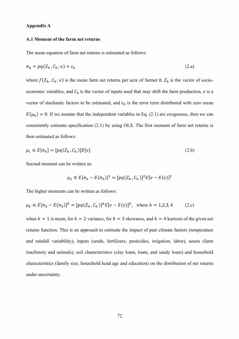
72
Appendix A
A.1 Moment of the farm net returns
The mean equation of farm net returns is estimated as follows:
𝜋 = 𝑝𝑞(𝑍 , 𝐶 ; 𝑒) + 𝜀 (2.a)
where 𝑓(𝑍 , 𝐶 ; 𝑒) is the mean farm net returns per acre of farmer ℎ, 𝑍 is the vector of socio-
economic variables, and 𝐶 is the vector of inputs used that may shift the farm production, 𝑒 is a
vector of stochastic factors to be estimated, and 𝜀 is the error term distributed with zero mean
𝐸(µ ) = 0. If we assume that the independent variables in Eq. (2.1) are exogenous, then we can
consistently estimate specification (2.1) by using OLS. The first moment of farm net returns is
then estimated as follows:
𝜇 ≡ 𝐸[𝜋 ] = [𝑝𝑞(𝑍 , 𝐶 )]𝐸[𝑒] (2.b)
Second moment can be written as:
𝜇 ≡ 𝐸[𝜋 − 𝐸(𝜋 )] = [𝑝𝑞(𝑍 , 𝐶 )] 𝐸[𝑒 − 𝐸(𝑒)]
The higher moments can be written as follows:
𝜇 ≡ 𝐸[𝜋 − 𝐸(𝜋 )] = [𝑝𝑞(𝑍 , 𝐶 )] 𝐸[𝑒 − 𝐸(𝑒)] , where 𝑘 = 1,2,3, 4 (2.c)
when 𝑘 = 1 is mean, for 𝑘 = 2 variance, for 𝑘 = 3 skewness, and 𝑘 = 4 kurtosis of the given net
returns function. This is an approach to estimate the impact of past climate factors (temperature
and rainfall variability), inputs (seeds, fertilizers, pesticides, irrigation, labor), assets (farm
machinery and animals), soil characteristics (clay loam, loam, and sandy loam) and household
characteristics (family size, household head age and education) on the distribution of net returns
under uncertainty.

73
Table 2.A1 Log-linear farm net returns function estimation
Variables Coefficients Std errors Constant 11.02943*** (0.46862) Credit_const −0.02956* (0.01550) Avg_Tem −0.03198* (0.01693) Avg_Rain −0.07297* (0.04136) tem_anomaly −0.45108 (1.52895) rain_anomaly −0.00324 (0.01045) HH_age −0.00131** (0.00051) Familysize −0.00687* (0.00385) Education 0.01132*** (0.00287) farm_size −0.00291** (0.00115) no_of_animal 0.01391** (0.00553) HH_fertilizers 0.00003*** (0.00000) HH_pesticides 0.00005*** (0.00001) HH_seed 0.00002*** (0.00000) HH_labour 0.00002*** (0.00000) HH_irrigation 0.00006*** (0.00001) Sandy loam −0.11277*** (0.02086) Clay loam 0.00205 (0.01894) Ext_services 0.02444* (0.01470) cc_shock 0.03912*** (0.01365) Xcotton 0.05215 (0.03465) Xrice 0.05581 (0.05337) agri_machinary 0.03977** (0.01575)
Note: The dependent variable is the natural logarithm of farm net returns. Standard errors are in parentheses. The reference region is mix cropping zone; the reference soil type is loam soil.
*** Significant at 1% level, ** significant at 5% level and * significant at 10% level.
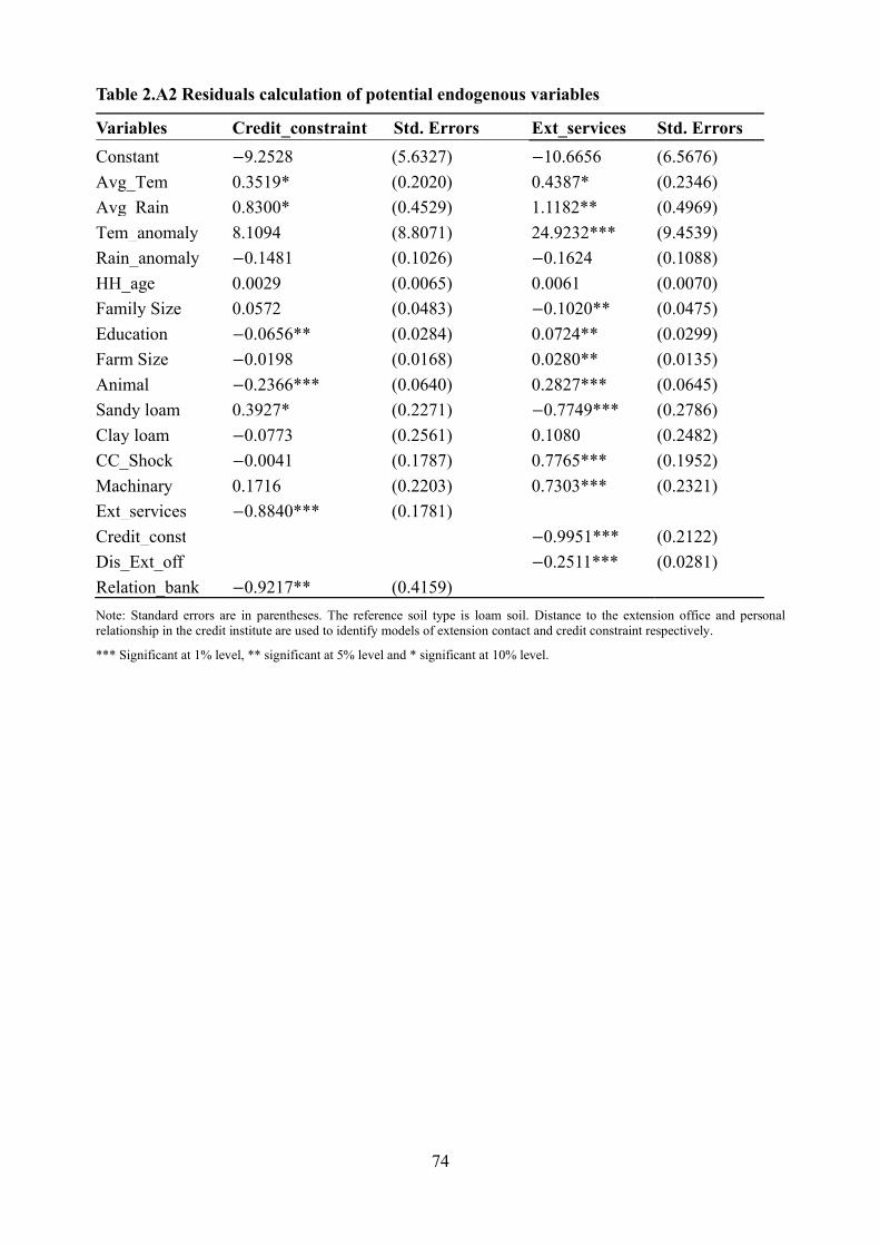
74
Table 2.A2 Residuals calculation of potential endogenous variables
Variables Credit_constraint Std. Errors Ext_services Std. Errors
Constant −9.2528 (5.6327) −10.6656 (6.5676)
Avg_Tem 0.3519* (0.2020) 0.4387* (0.2346)
Avg_Rain 0.8300* (0.4529) 1.1182** (0.4969)
Tem_anomaly 8.1094 (8.8071) 24.9232*** (9.4539)
Rain_anomaly −0.1481 (0.1026) −0.1624 (0.1088)
HH_age 0.0029 (0.0065) 0.0061 (0.0070)
Family Size 0.0572 (0.0483) −0.1020** (0.0475)
Education −0.0656** (0.0284) 0.0724** (0.0299)
Farm Size −0.0198 (0.0168) 0.0280** (0.0135)
Animal −0.2366*** (0.0640) 0.2827*** (0.0645)
Sandy loam 0.3927* (0.2271) −0.7749*** (0.2786)
Clay loam −0.0773 (0.2561) 0.1080 (0.2482)
CC_Shock −0.0041 (0.1787) 0.7765*** (0.1952)
Machinary 0.1716 (0.2203) 0.7303*** (0.2321)
Ext_services −0.8840*** (0.1781)
Credit_const −0.9951*** (0.2122)
Dis_Ext_off −0.2511*** (0.0281)
Relation_bank −0.9217** (0.4159)
Note: Standard errors are in parentheses. The reference soil type is loam soil. Distance to the extension office and personal relationship in the credit institute are used to identify models of extension contact and credit constraint respectively.
*** Significant at 1% level, ** significant at 5% level and * significant at 10% level.
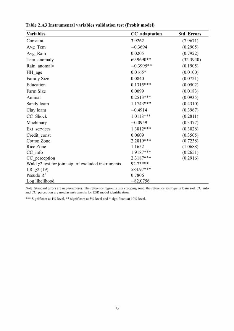
75
Table 2.A3 Instrumental variables validation test (Probit model)
Variables CC_adaptation Std. Errors
Constant 3.9262 (7.9671) Avg_Tem −0.3694 (0.2905) Avg_Rain 0.0205 (0.7922) Tem_anomaly 69.9690** (32.3940) Rain_anomaly −0.3995** (0.1905) HH_age 0.0165* (0.0100) Family Size 0.0840 (0.0721) Education 0.1315*** (0.0502) Farm Size 0.0099 (0.0183) Animal 0.2513*** (0.0935) Sandy loam 1.1743*** (0.4310) Clay loam −0.4914 (0.3967) CC_Shock 1.0118*** (0.2811) Machinary −0.0959 (0.3377) Ext_services 1.3812*** (0.3026) Credit_const 0.0609 (0.3505) Cotton Zone 2.2819*** (0.7238) Rice Zone 1.1652 (1.0688) CC_info 1.9187*** (0.2651) CC_perception 2.3187*** (0.2916) Wald χ2 test for joint sig. of excluded instruments 92.73*** LR χ2 (19) 583.97*** Pseudo R2 0.7806 Log likelihood −82.0756
Note: Standard errors are in parentheses. The reference region is mix cropping zone; the reference soil type is loam soil. CC_info and CC_perception are used as instruments for ESR model identification.
*** Significant at 1% level, ** significant at 5% level and * significant at 10% level.

76
Table 2.A4 Instrumental variables validation test non-adopters (OLS)
Variables Kurtosis VAR SK Net_returns
Constant −0.0439 (0.0310) −0.1833 (0.1393) 0.0385 (0.0661) 11.3391*** (0.8872)
Credit_const −0.0003 (0.0010) −0.0009 (0.0044) −0.0018 (0.0021) −0.0880*** (0.0287)
Avg_Tem 0.0016 (0.0011) 0.0069 (0.0050) −0.0016 (0.0024) −0.0195 (0.0319) Avg_Rain 0.0044 (0.0029) 0.0220* (0.0128) 0.0018 (0.0061) 0.0935 (0.0825)
Tem_anomaly 0.0361 (0.1132) 0.4836 (0.5080) −0.4876** (0.2413) −6.2313* (3.2488)
Rain_anomaly −0.0008 (0.0008) −0.0063* (0.0034) 0.0036** (0.0016) 0.0384* (0.0221)
HH_age −0.0000 (0.0000) −0.0000 (0.0002) 0.0001 (0.0001) −0.0007 (0.0011)
Family Size 0.0003 (0.0003) 0.0012 (0.0015) −0.0012* (0.0007) −0.0147 (0.0095)
Education −0.0002 (0.0002) −0.0007 (0.0009) 0.0004 (0.0004) 0.0529*** (0.0059)
Farm Size 0.0002 (0.0001) 0.0009 (0.0005) −0.0008*** (0.0002) −0.0208*** (0.0034)
Animal −0.0013*** (0.0005) −0.0045** (0.0022) 0.0023** (0.0011) 0.0514*** (0.0143)
Sandy loam 0.0044*** (0.0013) 0.0263*** (0.0059) −0.0044 (0.0028) −0.2945*** (0.0382)
Clay loam −0.0005 (0.0013) −0.0023 (0.0061) 0.0013 (0.0029) 0.1261*** (0.0391)
Ext_services 0.0008 (0.0012) −0.0009 (0.0052) 0.0028 (0.0025) 0.0733** (0.0292)
CC_Shock 0.0005 (0.0018) 0.0143* (0.0081) −0.0019 (0.0038) −0.1163** (0.0523)
Cotton Zone 0.0033 (0.0026) 0.0247** (0.0115) −0.0157*** (0.0054) −0.2423*** (0.0739)
Rice Zone 0.0019 (0.0041) 0.0133 (0.0184) −0.0194** (0.0088) −0.4389*** (0.1177)
Machinary −0.0002 (0.0014) −0.0031 (0.0063) 0.0004 (0.0030) 0.0498 (0.0405)
CC_info −0.0005 (0.0012) −0.0020 (0.0054) 0.0021 (0.0026) −0.0037 (0.0351)
CC_perception −0.0013 (0.0014) −0.0075 (0.0063) 0.0030 (0.0030) 0.0669 (0.0406)
Dis_Ext_off 0.0000 (0.0001) 0.0002 (0.0007) 0.0002 (0.0003) −0.0027 (0.0042)
Relativ_bank 0.0005 (0.0018) 0.0065 (0.0082) −0.0025 (0.0039) −0.0733 (0.0527)
F-test 0.45 [0.6363] 0.36 [0.6979] 0.23 [0.7936] 0.16 [0.8509]
Note: The reference region is mix cropping zone; the reference soil type is loam soil. CC_info and CC_perception are used as instruments for ESR model identification. Distance to the extension office and relative in the credit institute are used to identify residuals from extension contact and credit constraint, respectively. Standard errors are in parentheses. The p-values are given in square brackets.
*** Significant at 1% level, ** significant at 5% level and * significant at 10% level.
Table 2.A5 Instrumental variable correlation test
(1) (2) (3) (4) (5) (6) (7) (8)
Skewness (1) 1.0000
Net returns (2) 0.2425 1.0000
cc_info (3) 0.1054 0.2541 1.0000
cc_percep (4) 0.0141 0.2025 0.5894 1.0000
dis_ext (5) 0.0030 −0.1851 −0.1803 −0.1403 1.0000
Res_ext (6) 0.0348 0.1589 0.2075 0.1509 −0.0970 1.0000
Res_credit (7) −0.0326 −0.1171 −0.0536 −0.1155 0.0260 0.1410 1.0000
Relativ_bank (8) −0.1069 0.2124 −0.0099 −0.0824 0.0608 0.0229 −0.0090 1.0000

77
Fig. 2.A1 Kernel density plot for adopters and non-adopters (Net Returns)
0.5
11
.5kd
ensi
ty ln
_ne
t_re
turn
s
9.5 10 10.5 11 11.5 12Net Returns Distributions
adaptation Non-adaptation

78
Chapter 3
Climate Risk Management in Agricultural and Rural Household Welfare: Empirical
Evidence from Pakistan
Muhammad Faisal Shahzad and Awudu Abdulai
Department of Food Economics and Consumption Studies
Submitted to Journal of International Development
Abstract
In this paper, we investigate the determinants of farmers’ adaptation choices against climate
change and analyze the impact of these choices on farm households’ welfare. A recent farm-level
data from three agro-ecological zones of Pakistan are used to estimate a multinomial endogenous
switching regression for different climate-smart agriculture (CSA) practices, namely changing
inputs mix, change in cropping calendar, diversifying seed variety and soil and water conservation,
and the impact of each adopted practice on farm net returns and downside risk exposure. The
results show that adoption of different CSA practices is determined by average rainfall, ownership
of agricultural machinery, previous experience of climate-related shocks, education of household
head, access to climate change information, and climate change perception. The findings also
reveal that adoption of CSA practices positively and significantly improves the welfare of rural
farm households and reduces their exposure to downside risk and crop failure. The results further
revealed significant differences in the impacts of CSA practices adoption on farm net returns in
different agroecological zones and quantiles of plot sizes. Thus, policy efforts to scale-up adoption
of CSA practices should consider agroecological zone and farm size differences in addition to
enhancing farmer education, extension, and access to climate change information.
Keywords: Climate change, adoption, impact assessment, selectivity correction, rural welfare,
Pakistan.
JEL Codes: C21, C26, Q54, O33, D13.

79
3.1. Introduction
Climate change and extreme weather events are making the world weather uncertain and pose a
devastating direct effect on agriculture, making this business riskier (Beddington, 2011; Shannon
and Motha, 2015, Shahzad and Abdulai, 2020). Warm atmosphere, decrease in snowfall, rising
sea level, unpredicted changes in precipitation and greenhouse gas emissions are causing extreme
weather and climatic events (IPCC, 2013). The rise in temperature is the major driver of such
changes (Wolkovich et al., 2012). Climate change and extreme weather events are the major
threats to agriculture in the world, especially South Asian countries. Climate variability induces
challenges to achieving food security, poverty reduction and rural development in these countries
due to the vagaries of weather and other natural disasters such as extreme temperatures, extremely
erratic rainfall, floods and droughts, dust cyclones, pest infestation and crop diseases coupled with
low adoption rates of new technologies (IPCC, 2014). Variations in climate have a significant
impact on water resources, agriculture production, food supply, farmers’ wellfare and finally the
global economy (FAO, 2011; IPCC, 2012).
Climate-smart agriculture (CSA) has emerged as a framework for developing and implementing
robust agricultural systems, which simultaneously improve food security, living conditions in
rural areas, facilitate adaptation to climate change, and provide mitigation benefits (FAO, 2013).
The global community has recommended the incorporation of climate-smart agriculture (CSA)
practices into national development plans to mitigate the adverse impacts of climate change on
agriculture (IPCC, 2007; World Bank, 2010). Climate-smart agriculture practice is a practice on
the farm, which sustainably increases agricultural productivity, adapts and builds the resilience of
agricultural and food systems to climate change, and reduces greenhouse gas emissions from
agriculture (FAO, 2013). The CSA practices such as changing input mix and cropping calendar,
crop diversification, diversifying seed variety, crop rotation, soil and water conservation, using
improved seed variety, income diversification, crop and livestock integration and improving
80
irrigation efficiency are the strategies generally used to reduce climate change adverse effects
(Tubiello et al., 2008; Soglo and Nonvide, 2019).
It is projected that by the middle of the 21st century, the largest number of food-insecure people
will be found in South Asia due to the adverse effects of climate change (IPCC, 2014). Previous
studies have shown that adoption of CSA practices plays a significant role in increasing farm
productivity and household income, contributes to rural income growth, poverty reduction and
food security (Abid et al., 2016b; Iqbal et al., 2015; Ali and Erenstein, 2017; Khanal et al., 2018).
Moreover, adoption of CSA practices has been found to help smallholder farmers living in rural
areas overcome production and income risks (Mukasa, 2018; Hansen et al., 2019). For these
reasons, the significance of CSA practices in promoting farm households’ adoption of CSA
practices, improving their livelihood and welfare in South Asian countries has attracted
considerable attention from researchers and policymakers.
Although, most of the previous studies on adoption of climate change in the agricultural sector are
focused on developing countries in Africa. However, the literature on the adoption of climate
change perspectives in Pakistan is rare and few studies (e.g., Abid et al., 2016b; Iqbal et al., 2015)
have analyzed the impact of climate change adaptation from agricultural perspective. Abid et al.
(2016b) found that adaptation to climate change improves farm productivity and crop income,
while Iqbal et al. (2015) investigated farmers’ choices of adaptation such as varietal change,
delayed sowing and input intensification, using Heckman's Treatment Effects model, found a
significant and positive impact of adaptation choices on wheat crop net revenues in Pakistan.
Sabiha et al., (2017) concluded that high yielding varieties increase production efficiencies in
Bangladesh, while Veettil et al., (2016) found that adoption of Bt-technology reduced
environmental damage in India. Furthermore, divergent findings from these studies about
adaptation impact on farm performance offer motivation for further empirical assessment with
respect to topography and agroecology.

81
Despite the potential of CSA practices to enhance agricultural sustainability, adoption rates of
CSA practices in Pakistan are reported to be very low. FAO (2019) reports that adoption rate of
balance input use in irrigated area, use of heat and drought tolerant varieties in rainfed area, soil
and water conservation practices for cotton farmers are less than 30%. The reasons for low
adoption rates in Pakistan appear to be mixed. For instance, Salman et al., (2018) report that many
farmers in Pakistan do not consider climate change as a potential threat to agriculture and therefore
do not see the need to change their farming practices. Also, policy implementation regarding
adaptation to climate change is weak and entails strong integration with other policies, institutions
and financial funding in support of promoting CSA practices (FAO, 2019). Further, some studies
attribute the low adoption rates to knowledge gap between researchers and policy-makers, which
needs to be bridged for the development of a comprehensive plan of CSA practices for adoption
(Ali et al., 2019).
We define climate-smart agriculture practice broadly to include adoption strategies such as
changing cropping calendar, diversify seed varieties, changing input mix and soil and water
conservation (FAO, 2013). The present study contributes to the growing literature on the adoption
of CSA practices, by examining the factors influencing these practices, as well as estimating the
impact of these CSA adoption choices on farm net returns and downside risk exposure. In addition
to the country-specific contribution to literature, we also extend the cropping mixed analysis by
moving away from mono-cropping analysis to mixed-cropping that exploits the interlink benefits
from multiple climate-smart practices. Very few studies have examined the adoption impacts of
multiple CSA practices on farmers’ productivity and exposure to risk, though from mono-
cropping perspective (Di Falco and Veronesi, 2013; Iqbal et al., 2015). However, the conclusion
based on a single crop may under or overestimate the real impacts of adoption for several reasons.
For instance, if a farmer in mixed crop setting changes the input mix for rice crop it may increase
or decrease the production of other crops on the field. In the same way, for a coherent

82
understanding, if multi-product farmer applies soil and water conservation techniques for wheat
crop, it might offer benefit to oilseed crops in the same season and increase yield of cotton, rice,
maize in the following season, which may not be captured if a researcher considers only wheat
yield leaving out other crops. Furthermore, there might be a negative interaction between crops in
mixed setting, where increase in yield of one crop may lead to decrease the yield of other crops
(Tessema et al., 2015).
Since smallholder farmers predominantly cultivate mixed-crops as part of risk minimization
strategy, we depart from the previous studies that analysed farm level risk based on monocropping
cropping context (e.g., Kassie et al., 2014; Di Falco and Veronesi, 2013) by considering the multi-
cropping nature of farming in Pakistan in our analysis. Furthermore, we examine factors that
influence farmer’s choice of different CSA practices, since understanding linkages between these
choices and farm outcomes can also provide significant information to policymakers on possible
promotion and scaling up of different CSA practices. Analysis of CSA adoption choices may also
provide insights into which adaptation choice is a more effective option for multi-product farmers.
To the extent that CSA overlaps other development goals such as food security, poverty reduction,
and rural development (Vale, 2016; Abdulai, 2018), results obtained from this study can inform
climate change policy design, especially in developing country settings similar to Pakistan. To
achieve our research objective, we combine spatial climate data with recent survey data from three
important agro-ecological zones of the Punjab province of Pakistan to estimate the multinomial
endogenous switching regression (MESR) and implement counterfactual analysis. For robustness
check, we employ multivariate treatment effect regression to compare the results.
The rest of the paper is organized as follows. The next section presents the data and descriptive
statistics. The third section presents methodology which discusses the conceptual framework as
well as the empirical analytical approach. The fourth section addresses the results and discussions,
while the final section presents the conclusion and policy implications of the study.

83
3.2. Data and descriptive statistics
The cross-sectional data used in this study come from a survey conducted between January and
March 2017 in Pakistan by the authors. A farm household sampling frame was developed to ensure
representation for the study region. For the data collection, we considered the cropping pattern,
agricultural activities, percent of cultivated land area, climate, and weather variability within agro-
ecological zones. The data were collected from six administrative units of the Punjab province.
Three important zones (cotton zone, rice zone, and mix cropping zone) were selected purposively
based on climatic and agro-ecological cropping patterns (see Fig. 3.1). The selected zones have
different climatic conditions and cropping patterns. A multi-stage stratified random sampling
procedure was applied to collect data from farmers. During the first stage, three zones from the
Punjab province were selected purposively on a climate and agro-ecological basis. In the second
stage, two districts from each zone were randomly selected. In the third stage, two tehsils were
randomly chosen from each district, then three villages were randomly selected from each tehsil.
In the fifth stage, fifteen farmers were randomly selected from each village. Overall, 540 farmers
were interviewed for the data collection. In total, they were cultivating 748 agricultural plots. A
structured questionnaire was used to collect socio-economic and farm-level information from the
respondents, through face to face interviews.
The collected data were comprehensive, which include information on farm households,
agricultural practices, production and costs, irrigation water use, access to extension, social
networking, perceptions about climate change and climate risks, responses to climate change,
credit access, farm and household assets, other income sources, consumption, and expenditure.
One section of the questionnaire was particularly designed to capture climate change perceptions
and climate risks and understanding of adaptation responses against climate change. Questions
were included to ask the farmers whether they have noticed long term changes in temperature and
precipitation over the last twenty years. Secondary information related to temperature and rainfall

84
was collected from the National Center for Environmental Prediction (NCEP) and World Weather
Online. The collected information ranges from 1979 to 2016, the same year in which we obtained
data from farmers. It was converted from monthly to yearly averages and calculate daily average
rainfall and daily average temperature over the years at household level. As the Punjab province
is mostly flat, we used the inverse distance method of spatial interpolation to calculate location-
specific farm-level temperature and rainfall. For this purpose, we used the global positioning
(GPS) system to record the farm location (elevation, longitude, and latitude) during the data
collection. The recorded farm locations were employed in interpolation analysis to obtain
information on farm-level temperature and rainfall. Subsequently, we calculated the temperature
and rainfall anomalies, taking 2016 as a base year in which we collected primary data from
farmers.
Evidence from the data shows that CSA practices were mainly related to farm net returns measures
(see Table 3.1). The data also indicate that at least one CSA practice was adopted on 54% of
cultivated plots, with no adoption taking place on the remaining 46 percent cultivated plots. In
particular, diversification of seed variety was used as a strategy on 11% of plots, changing
cropping calendar on 14%, changing input mix on 13% of plots, while soil and water conservation
measures were adopted on 15% of cultivated plots. Thus, we identify four main adaptation
strategies (1) seed variety diversification, (2) changing cropping calendar, (3) changing input mix,
and (4) soil and water conservation.7 The average daily temperature and rainfall are recorded at
27°C and 1 millimeter over the last 38 years, respectively. Temperature and rainfall shocks are
captured in rainfall anomalies. Temperature anomaly is positive in the area showing that on
average, temperature anomalies are recorded 0.22°C, while on an average rainfall anomaly shows
7 As we have limited data (total number of adopted plots are 401), the adopters of multiple adaptation strategies range between 5-40 that is small in number. With this small number of observations MESR generates inconsistent estimates because with small number of observations the identification of the covariance matrix between all model residuals may become intractable. Therefore, we considered these main CSA practices in the analysis.

85
a reduction of rainfall by 0.37 millimeters. On average, 28 percent of farmers are credit
constrained with an average plot holding of 5.9 acres. On average, 25 percent of farmers have
agricultural machinery at their farms. In the past three years, about 39 percent of farmers were
exposed to climate-related shocks such as floods, droughts, pest infestation, and diseases.
Furthermore, we also captured the plot-variant characteristics such as soil fertility, erosion, and
distance from farmers’ houses to the plot. On average, 43 percent of plots are fertile, with an
average distance of 2 km between farmer’s house and the plot. On average, 21 percent of plots
face moderate to severe erosion.
Fig. 3.1 Map of Pakistan showing study area and data collection sites

86
Table 3.1 Definition and descriptive statistics of selected variables
aAnomaly= (current year mean -long term mean)/long term mean
b 1 acre= 0.405 hectare
c PKR (Pakistani Rupee) is Pakistani currency (1 $=104.67 PKR during the year of data collection).
Variables Definition Mean SD No adaptation 1 if farmer chose not to adapt to climate change, 0 otherwise 0.464 0.499
Seed variety diver. 1 if farmer chose seed varieties diversification at the farm, 0 otherwise 0.112 0.316
Cropping calendar 1 if farmer chose to change sowing dates of crops, 0 otherwise 0.142 0.349
Input mix 1 if farmer chose to change input mix, 0 otherwise 0.131 0.338
SWC 1 if farmer chose to adopt soil and water conservation, 0 otherwise 0.151 0.358
Credit_const 1 if farmer is liquidity constraint, 0 otherwise 0.282 0.450
Avg Tem Average annual daily temperature in (degrees Celsius) 27.334 1.110
Avg Rain Average annual daily rain (millimeters) 0.639 0.553
Int TxR Product of average daily temperature and average daily rainfall 16.882 13.821
Tem anomaly Change in temperature relative to baselinea (number) 0.217 0.032
Rain anomaly Change in rainfall relative to baseline (number) −0.369 0.194
HH age Household head age (years) 47.219 11.259
Family size Number of persons residing in a household (number) 6.147 2.223
Education Number of schooling years household head completed (years) 6.524 4.293
Plot size Total number of acres a farm household cultivate at one place (acresb) 5.937 3.580
Herd size Number of animals a farm household owns (number) 4.052 2.360
Machinery 1 if farmer has own farm machinery, 0 otherwise 0.247 0.432
cc_shock 1 if farmer exposed to climate-related shocks in the past three years, 0 otherwise
0.386 0.487
Ext services 1 if farmer has contact with govt. extension agent, 0 otherwise 0.290 0.454
Cotton zone 1 if farmer resides in cotton growing zone, 0 otherwise 0.310 0.463
Rice zone 1 if farmer resides in mix cropping zone, 0 otherwise 0.334 0.472
Mix zone 1 if farmer resides in rice growing zone, 0 otherwise 0.356 0.479
Fertile Mean fertility=1 if soil is fertile, 0 otherwise 0.434 0.437
Erosion Mean erosion=1 if agricultural plot has moderate to severe erosion, 0 otherwise
0.210 0.532
Plot distance Mean distance to agricultural plot from farmer’s house (km) 2.122 1.421
cc info 1 if a farmer receives current information related to climate change, 0 otherwise
0.373 0.484
cc perception 1 if farmer perceives changes in climate change, 0 otherwise 0.356 0.479
Farm net returns Gross farm revenue minus variable costs (Thousand PKRc) 59.119 17.569
Skewness Third central movement of the farm net returns function −0.001 0.013
Total no. of obs. 748
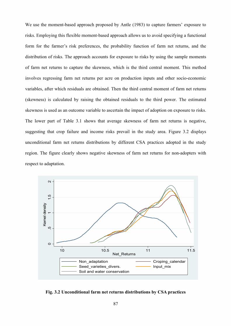
87
We use the moment-based approach proposed by Antle (1983) to capture farmers’ exposure to
risks. Employing this flexible moment-based approach allows us to avoid specifying a functional
form for the farmer’s risk preferences, the probability function of farm net returns, and the
distribution of risks. The approach accounts for exposure to risks by using the sample moments
of farm net returns to capture the skewness, which is the third central moment. This method
involves regressing farm net returns per acre on production inputs and other socio-economic
variables, after which residuals are obtained. Then the third central moment of farm net returns
(skewness) is calculated by raising the obtained residuals to the third power. The estimated
skewness is used as an outcome variable to ascertain the impact of adoption on exposure to risks.
The lower part of Table 3.1 shows that average skewness of farm net returns is negative,
suggesting that crop failure and income risks prevail in the study area. Figure 3.2 displays
unconditional farm net returns distributions by different CSA practices adopted in the study
region. The figure clearly shows negative skewness of farm net returns for non-adopters with
respect to adaptation.
Fig. 3.2 Unconditional farm net returns distributions by CSA practices
0.5
11.5
2K
ern
el d
ensi
ty
10 10.5 11 11.5Net_Returns
Non_adaptation Croping_calendarSeed_varieties_divers. Input_mixSoil and water conservation

88
Table 3.2 Summary statistics of the variables used for the CSA adopters and non-adopters
Variables Non-adaptation
(𝒏 = 𝟑𝟒𝟕) Seed variety diver.
(𝒏 = 𝟗𝟖) Cropping Calendar
(𝒏 = 𝟏𝟎𝟔) Input mix (𝒏 = 𝟖𝟒)
SWC (𝒏 = 𝟏𝟏𝟑)
Mean SD Mean SD Mean SD Mean SD Mean SD Credit_const 0.343 0.475 0.225 0.419 0.189 0.393 0.298 0.460 0.221 0.417 Avg Tem 27.249 1.118 27.392 1.140 27.435 1.055 27.341 1.149 27.442 1.079 Avg Rain 0.670 0.572 0.630 0.553 0.587 0.509 0.653 0.565 0.590 0.527 int TxR 17.642 14.246 16.670 13.832 15.605 12.780 17.248 14.150 15.661 13.226 Tem anomaly 0.213 0.030 0.218 0.032 0.220 0.032 0.219 0.033 0.223 0.034 Rain anomaly −0.353 0.188 −0.387 0.194 −0.386 0.195 −0.375 0.204 −0.384 0.206 HH age 47.228 11.468 47.122 11.268 46.226 10.727 48.655 11.177 47.142 11.234 Family size 5.968 2.139 6.112 2.252 6.330 2.114 6.571 2.495 6.239 2.316 Education 4.559 3.810 8.071 3.923 8.151 3.685 8.607 4.186 8.142 4.073 Plot size 5.899 3.793 5.715 3.296 6.259 3.447 6.015 3.145 5.885 3.609 Herd size 3.856 2.152 4.306 2.526 4.387 2.635 3.964 2.686 4.186 2.266 Machinery 0.058 0.233 0.480 0.502 0.321 0.469 0.441 0.499 0.416 0.495 cc_shock 0.199 0.400 0.653 0.478 0.557 0.499 0.393 0.491 0.566 0.498 Ext services 0.285 0.452 0.316 0.467 0.302 0.461 0.250 0.436 0.301 0.461 Xcotton 0.334 0.472 0.306 0.463 0.274 0.448 0.310 0.465 0.274 0.448 Xrice 0.257 0.437 0.398 0.492 0.387 0.489 0.393 0.491 0.425 0.497 Xmix 0.409 0.492 0.296 0.459 0.340 0.476 0.298 0.460 0.301 0.461 Fertile 0.337 0.405 0.489 0.447 0.510 0.444 0.556 0.452 0.525 0.451 Erosion 0.323 0.708 0.105 0.260 0.130 0.314 0.131 0.281 0.089 0.234 Plot_distance 2.452 1.603 1.594 1.127 1.892 1.097 1.967 1.171 1.895 1.256 cc info 0.020 0.141 0.633 0.485 0.689 0.465 0.726 0.449 0.673 0.471 cc perception 0.023 0.150 0.694 0.463 0.585 0.495 0.667 0.474 0.637 0.483 Farm net returns
48.571 13.782 68.543 16.015 67.118 15.021 68.569 15.591 68.810 14.610 Skewness −0.005 0.016 0.001 0.004 0.002 0.009 0.002 0.004 0.003 0.006

89
Table 3.2 presents the summary statistics of the variables used in the analysis, classified into
CSA practices by adopters and non-adopters. The table shows that adopters of CSA practices
earned higher farm net returns and reduced their exposure to income risks (positive skewness)
than non-adopters (negative skewness) in all adoption cases.
3.3. Methodology
3.3.1. Conceptual framework
The conceptual framework used in the analysis is based on the assumption that farmers normally
made adoption decisions from a given set of CSA adoption choices in order to minimize the
adverse effects of climate change. We assume a multi-product farmer producing under uncertain
climate scenarios with different choices of adaptation strategies. As indicated previously, the
specific CSA practices considered in this study are changes in cropping calendar, diversifying
seed variety, changing input mix, and soil and water conservation. Previous studies have linked
adoption of planting dates to farmers’ adaptation behavior (Abid et al., 2016b; Iqbal et al., 2015;
Di Falco and Veronesi, 2014). Diversification of seed varieties includes the use of drought-
resistant and early maturing varieties that enable farmers to cope with erratic rainfall or very low
rainfall (Kassie et al., 2017). Changing the input mix includes changing fertilizer types and
quantities, changes in pesticide use, changing irrigation, changing the use of herbicides or
weedicides, and micro-nutrients (Arslan, 2015). Soil and water conservation refers to soil erosion
reduction and other measures to prevent soil and nutrient loss, and conserve soil moisture with
practices such as practicing crop rotation to prevent nutrient loss in the soil, sowing cover crops
to fix nitrogen in the soil, planting on ridges, making soil bunds at an appropriate distance to
reduce soil erosion and water loss, planting shade trees to reduce evapotranspiration, and use of
farmyard manure with minimum tillage which increases the soil’s water holding capacity
(Hudson, 1987; Gicheru et al., 2004).
We assume that farmers are risk-averse and consider farm net benefits from an adaptation strategy
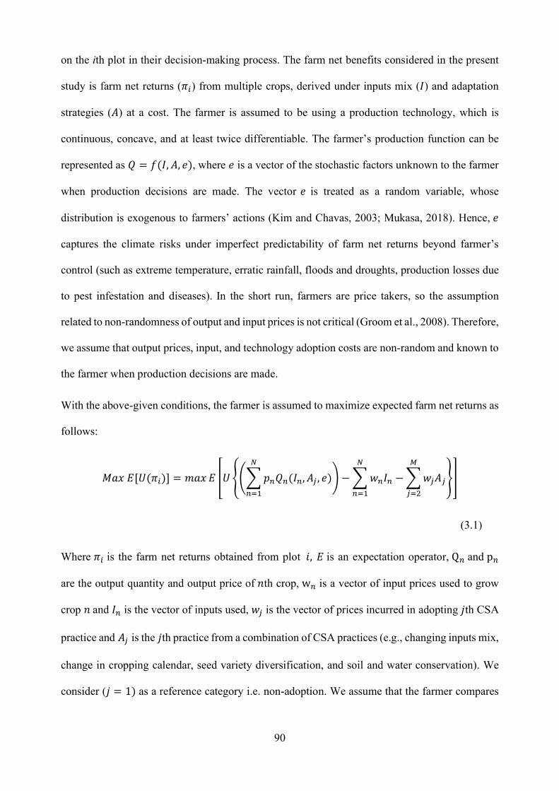
90
on the ith plot in their decision-making process. The farm net benefits considered in the present
study is farm net returns (𝜋 ) from multiple crops, derived under inputs mix (𝐼) and adaptation
strategies (𝐴) at a cost. The farmer is assumed to be using a production technology, which is
continuous, concave, and at least twice differentiable. The farmer’s production function can be
represented as 𝑄 = 𝑓(𝐼, 𝐴, 𝑒), where 𝑒 is a vector of the stochastic factors unknown to the farmer
when production decisions are made. The vector 𝑒 is treated as a random variable, whose
distribution is exogenous to farmers’ actions (Kim and Chavas, 2003; Mukasa, 2018). Hence, 𝑒
captures the climate risks under imperfect predictability of farm net returns beyond farmer’s
control (such as extreme temperature, erratic rainfall, floods and droughts, production losses due
to pest infestation and diseases). In the short run, farmers are price takers, so the assumption
related to non-randomness of output and input prices is not critical (Groom et al., 2008). Therefore,
we assume that output prices, input, and technology adoption costs are non-random and known to
the farmer when production decisions are made.
With the above-given conditions, the farmer is assumed to maximize expected farm net returns as
follows:
𝑀𝑎𝑥 𝐸[𝑈(𝜋 )] = 𝑚𝑎𝑥 𝐸 𝑈 𝑝 𝑄 (𝐼 , 𝐴 , 𝑒) − 𝑤 𝐼 − 𝑤 𝐴
(3.1)
Where 𝜋 is the farm net returns obtained from plot 𝑖, 𝐸 is an expectation operator, Q and p
are the output quantity and output price of 𝑛th crop, w is a vector of input prices used to grow
crop 𝑛 and 𝐼 is the vector of inputs used, 𝑤 is the vector of prices incurred in adopting 𝑗th CSA
practice and 𝐴 is the 𝑗th practice from a combination of CSA practices (e.g., changing inputs mix,
change in cropping calendar, seed variety diversification, and soil and water conservation). We
consider (𝑗 = 1) as a reference category i.e. non-adoption. We assume that the farmer compares

91
the farm net returns from adopting 𝑗th CSA practice 𝐴 for plot i and the farm net returns obtained
from non-adoption 𝐴 . A risk-averse farmer will adopt 𝑗th CSA practice if the expected utility of
farm net returns with adoption 𝐸[𝑈(𝐴 )] is greater than the expected utility without
adoption 𝐸[𝑈(𝐴 )]. This can be expressed as 𝐸[𝑈(𝐴 )] − 𝐸[𝑈(𝐴 )] > 0.
3.3.2. Empirical Strategy
Given that farmers self-select into adoption of climate-smart agriculture (CSA) practices, selection
bias may arise due to observed and unobserved characteristics. Therefore, analyzing impact of
adoption using ordinary least square (OLS) might lead to biased and inconsistent estimates. To
assess the decision of farmers to adopt different CSA practices, the present study employs a
multinomial endogenous switching regression (MESR) approach. The MESR model is a two-step
estimation procedure that considers the selection bias correction among all alternate choices in
question (Bourguignon et al., 2007; Di Falco and Veronesi, 2013). In the first step, factors
affecting the adoption of CSA practices are considered. In the second step, consistent estimates of
parameters of all explanatory variables of interest are evaluated to identify impacts of these
variables on outcomes of interest (mean farm net returns and skewness of farm returns). Based on
these consistent estimates, the outcome equations can be specified.
First stage: Selection Model of Climate-Smart Farm Practices
As mentioned above, the farmer adopts CSA practices, if the expected farm net benefits from
adoption are positive. Given that the expected farm net benefits are unobservable, we can represent
it with a latent variable 𝐴∗ which can be expressed as a function of observed (𝑍 ) and unobserved
(𝜁 ) characteristics as follows:
𝐴∗ = 𝑍 𝛾 + 𝜁 (3.2)
where 𝑗 represents different CSA practices, such that 𝑗 = 1, 2, 3, … , 𝑀.
Let 𝐴 be an index of a set of CSA practices choices that a farmer can decide to implement at plot
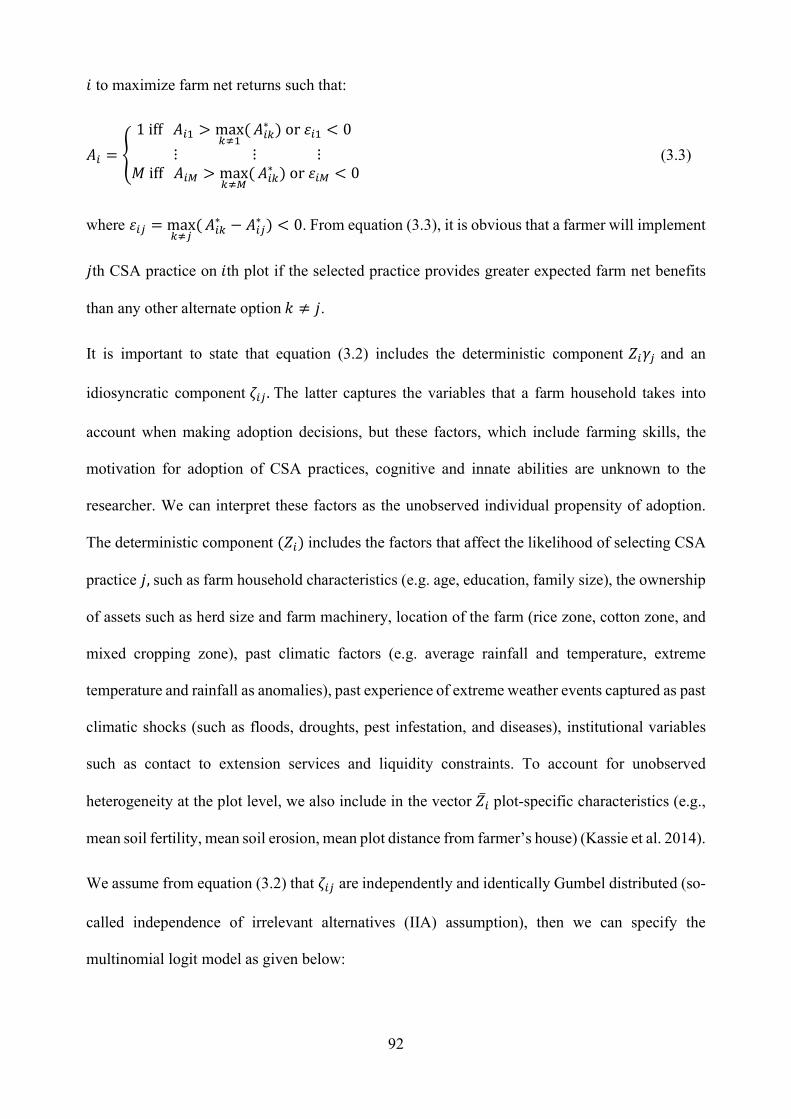
92
𝑖 to maximize farm net returns such that:
𝐴 =
1 iff 𝐴 > max( 𝐴∗ ) or 𝜀 < 0
⋮ ⋮ ⋮𝑀 iff 𝐴 > max( 𝐴∗ ) or 𝜀 < 0
(3.3)
where 𝜀 = max( 𝐴∗ − 𝐴∗ ) < 0. From equation (3.3), it is obvious that a farmer will implement
𝑗th CSA practice on 𝑖th plot if the selected practice provides greater expected farm net benefits
than any other alternate option 𝑘 ≠ 𝑗.
It is important to state that equation (3.2) includes the deterministic component 𝑍 𝛾 and an
idiosyncratic component 𝜁 . The latter captures the variables that a farm household takes into
account when making adoption decisions, but these factors, which include farming skills, the
motivation for adoption of CSA practices, cognitive and innate abilities are unknown to the
researcher. We can interpret these factors as the unobserved individual propensity of adoption.
The deterministic component (𝑍 ) includes the factors that affect the likelihood of selecting CSA
practice 𝑗, such as farm household characteristics (e.g. age, education, family size), the ownership
of assets such as herd size and farm machinery, location of the farm (rice zone, cotton zone, and
mixed cropping zone), past climatic factors (e.g. average rainfall and temperature, extreme
temperature and rainfall as anomalies), past experience of extreme weather events captured as past
climatic shocks (such as floods, droughts, pest infestation, and diseases), institutional variables
such as contact to extension services and liquidity constraints. To account for unobserved
heterogeneity at the plot level, we also include in the vector �̅� plot-specific characteristics (e.g.,
mean soil fertility, mean soil erosion, mean plot distance from farmer’s house) (Kassie et al. 2014).
We assume from equation (3.2) that 𝜁 are independently and identically Gumbel distributed (so-
called independence of irrelevant alternatives (IIA) assumption), then we can specify the
multinomial logit model as given below:

93
𝑃 = 𝑃 𝜀 < 0 𝑍 , �̅� = ( )
∑ ( ) , where 𝑗 = 1, 2, 3, … , 𝑀 (3.4)
The farmer chooses CSA practice 𝑗 among any other alternative 𝑘, if and only if 𝐴 >
𝑚𝑎𝑥 (𝐴 ). By using this expression, consistent maximum likelihood estimates of 𝛾 and 𝜕
can be obtained. Furthermore, we perform a Wald test of the joint significance of 𝜕 to determine
the effect of plot-level heterogeneity or the Mundlak effect (Mundlak, 1978).
Second stage: Multinomial Endogenous Switching Regression (MESR) Model
To examine the impact of adoption of CSA practices on outcome variables, we assume that
outcomes from multi-crops production are a linear function of the vector of explanatory variables.
We can write the outcome function as:
Regime 1: 𝑦 = 𝑋 𝛽 + 𝑋 𝜃 + 𝜇 , if 𝐴 = 1 (3.5a)
⋮ ⋮ ⋮ , ⋮ ⋮
Regime M: 𝑦 = 𝑋 𝛽 + 𝑋 𝜃 + 𝜇 , if 𝐴 = 𝑀 (3.5m)
where 𝑦 is the outcome of interest (farm net returns or skewness of farm net returns distribution)
from adoption of CSA practice 𝑀 among 𝑗 different alternatives based on the utilities such as non-
adaptation (𝑗 = 1), changing input mix (𝑗 = 2), changing cropping calendar (𝑗 = 3), varieties
diversification (𝑗 = 4), and soil and water conservation (𝑗 = 5); β and 𝜃 are the parameters to be
estimated, 𝜇 is the error term with zero mean and constant variance i.e. 𝜇 (0, 𝜎 ). The vector
𝑋 contains all control variables of interest such as household characteristics, ownership of assets,
location of the farm, past climatic factors, past experience of extreme weather events captured as
past climate shock, access to extension services and liquidity constraint. The vector 𝑋 comprises
mean soil characteristics, mean erosion and mean distance to the farm plot which are also included
in �̅� .
As mentioned above, farmers self-select themselves into the adoption of CSA practices;
consequently, the problem of selection bias may arise. Thus, there is a possibility that

94
unobservable characteristics may simultaneously affect both error terms in equations (3.4) and
(3.5a-3.5m), i.e. 𝑐𝑜𝑟𝑟(𝜁 , 𝜇 ) ≠ 0 . When this occurs, the estimates of 𝛽 and 𝜃 from the
ordinary least squares (OLS) may not be consistent. We employ a model proposed by
Bourguignon et al., (2007) to correct this potential inconsistency (selection bias). This model takes
into account the potential correlation between the error terms 𝜁 and 𝜇 . To overcome potential
inconsistency, we define the standard normal variables given below:
𝜁∗ = 𝐽 𝜁 = Φ {𝑔 𝜁 }, where 𝑗 = 1, 2, 3, . . . , 𝑀 (3.6)
For each 𝑗, we assume that the expected values of 𝜇 and 𝜁∗ are linearly related. Under a classical
assumption, it holds that 𝜇 is normal and (𝜇 , 𝜁∗ ) is bivariate normal for any adoption category 𝑗.
If 𝜌 represents the correlation between 𝜇 and 𝜁∗ , then to derive the selection bias-corrected
outcome equations, we can express the 𝜇 in the following linear combination:
𝐸 𝜇 𝜁 . . . 𝜁 = 𝜎 ∑ 𝜌 𝜁∗ (3.7)
Taking into account the above expression and following Bourguignon et al., (2007), we derive the
selection bias-corrected equations which can be used to estimate the consistent 𝛽 in the farm net
returns equations (3.5a)-(3.5m). The corrected equations can be specified as follows:
Regime 1: 𝑦 = 𝑋 𝛽 + 𝑋 𝜃 + 𝜎 𝜌 𝑚(𝑃 ) + ∑ 𝜌 𝑚(𝑃 ) + 𝜔 , if 𝐴 = 1 (3.8a)
⋮ ⋮ ⋮ , ⋮
Regime M: 𝑦 = 𝑋 𝛽 +𝑋 𝜃 + 𝜎 𝜌 𝑚(𝑃 ) + ∑ 𝜌 𝑚(𝑃 ) + 𝜔 , if 𝐴 = 𝑀 (3.8m)
Where 𝜆 = ∑ 𝜌 𝑚(𝑃 ) + 𝑚(𝑃 )( )
refers to inverse mills ratio computed from
estimated probabilities of MNL model in Eq. (3.4), 𝑚(𝑃 ) and 𝑚 𝑃 are conditional
expectations of 𝜁 and 𝜁 , which are used to correct selectivity bias, 𝜌 is the coefficient of
correlation between 𝜇 and 𝜁 , 𝜎 is the standard deviation of disturbance terms from net returns
equations and 𝜔 is the error term. From Eqs. (3.8a and 3.8m), it implies that the number of bias

95
correction terms in each equation are equal to the number of total adoption choices in question.
Therefore, this method provides efficient estimates compared to available methods.8
In the estimation, 𝑍 from the selection equation and 𝑋 from the outcome equations are
overlapping. In this case, proper model identification is required. Thus, to ensure model
identification, we need to have instruments that directly affect the selection decision at first stage
but does not affect the outcome variables in the second stage. We use access to climate change
information and perception as instrumental variables. Access to climate-specific information is
expected to enhance farmers’ understandings about climate change and directly influence their
adoption decisions (Issahaku and Abdulai, 2019). On the otherhand, perceptions and expectations
of future events may shape behavior, feelings and thoughts (Almlund et al., 2011) and are assumed
to be good predictor of economic behavior. Indigenous knowledge of farmers also influences
climate change perception behavior (Paudel et al., 2019). However, their validity may depend on
the methods used to elicit such opinions and might raise the concerns of possible reverse causality
(Delavende et al., 2011). In the present study, climate change perception is determined based on
the farmers’ experiences of past twenty years. Moreover, we perform Wald test for joint
significance of the excluded instruments, which shows that these instrumental variables jointly
and significantly influence adoption decisions of all four CSA practices (see lower part of Table
3.3). We also perform F-test for the excluded instruments that indicate instrumental variables do
not significantly affect outcome variables of farmers that did not adopt (see Table 3.B2 and 3.B3
in Appendix B). Hence, the results from both regressions confirm that climate change information
and perception are valid instruments (Issahaku and Abdulai, 2019; Di Falco et al., 2011). Adding
8 Previous literature on selection bias correction for the MNL model shows that Lee (1983) estimated only one correction term ζ − ζ for the selection bias correction for all choices, while Dubin and McFadden (1984) estimated (M-1) choices as to
selection bias correction. Another method also provided by Dahl (2002) for selection bias correction, which is suitable when a large number of observations are available and the choices of adoption in the selection model are small. On the other hand, we have a small number of observations available in which the identification of the covariance matrix between all model residuals may become intractable. However, Bourguignon et al., (2007) show that their method is more robust than previous methods.

96
these instruments to equation (3.2), can be specified as follows:
𝐴∗ = 𝑍 𝛾 + �̅� 𝜕 + 𝐼 𝜑 + 𝜏 (3.9)
where 𝐼 indicates the set of instrumental variables used to identify the MNL model, 𝜑 is the
parameters of the instrumental variables and 𝜏 is the error term with zero mean and constant
variance.
Another issue that deserves attention is the potential endogeneity of extension contact and credit
constraint variables in the selection equation. This is because extension service officers may
provide information related to particular CSA practices and farmers adopt these practices against
climate change for better farm production. Credit constraint variable is potentially endogenous
because non-adopters might be more prone to lower incomes, which worsen their credit
worthiness, and hence their liquidity status. This study applies control function approach
suggested by Murtazashvili and Wooldridge, (2016) to account for potential endogeneity arising
from these variables. In the control function approach, the potentially endogenous variables
(extension contact and liquidity constraint) are specified as a function of all other variables used
in the selection equation in addition to instrumental variables. As both of these variables are
dichotomous in nature, we estimate first-stage probit models of these variables to calculate
generalized residuals and predicted values of these variables by using the distance from local
agricultural advisory office and personal relationship in the credit institute as instruments,
respectively. Distance from a local advisory office is a good predictor of extension contacts and
expected to negatively affect the extension services, but it is not expected to affect the personal
characteristics of farm households such as motivation of adoption and innate abilities that would
affect farm net returns. Thus, distance from a local advisory office is expected to correlate with
extension contacts, but it is exogenous to the omitted variables contained in the error term
(Cawley, et al., 2018). Moreover, the location of farms in Pakistan is not a conscious choice where
to locate but is largely due to inheritance, thus the distance to the local advisory office is

97
exogenous. Interpersonal relationship in the credit institute is directly influenced by liquidity
constraint of a farmer because the personal relationship with an individual in the credit institute
eases the loan application process and reduces the time of obtaining loan due to knowledge of
application procedure, thereby expected to affect credit constraint negatively. This interpersonal
relationship is also exogenous to the farmer’s personal characteristics, and do not influence
adoption and outcome variables. Moreover, it is evident from F-test (see Tables 3.B2 and 3.B3)
in Appendix B) that these instruments are not significant for non-adopters. Also, the correlation
matrix (see Table 3.A8 in the Appendix B) shows that these instruments uncorrelated with
outcome variables and other instruments used for model identification, signifying the validity of
these instruments. The obtained generalized residuals from first stage probit regression serves as
a control function in the selection equation, while in second stage estimation, we used the
predicted values of these variables, enabling the consistent estimation of the potentially
endogenous variables in the MESR model (Murtazashvili and Wooldridge, 2016).
3.3.3. Counterfactual analysis and average treatment effects on the treated (ATT)
Following Heckman et al. (2001), we estimate the treatment effects on the treated. We can
compare the farm net returns of adopters to the counterfactual farm net returns of non-adopters
with the same observable characteristics. As unobserved heterogeneity in the decisions of adapting
𝑗th CSA practices also affects the farm net returns causing selection bias that cannot be ignored.
Therefore, we used the MESR model to account for selection bias arising from unobserved
heterogeneity in the sample. We estimate farm net returns of adopters which is in our case (𝑗 =
2, . . . , 𝑀) with 𝑗 = 1 as the base category, such that:
𝐸(𝑦 |𝐴 = 2) = 𝑋 𝛽 +𝑋 𝜃 + 𝜎 𝜆 (3.10a)
⋮ ⋮ ⋮ ⋮
𝐸(𝑦 |𝐴 = 𝑀) = 𝑋 𝛽 +𝑋 𝜃 + 𝜎 𝜆 (3.10m)
The counterfactual case that adopters did not adopt CSA practices (𝑗 = 1) can be stated as:

98
𝐸(𝑦 |𝐴 = 2) = 𝑋 𝛽 + 𝑋 𝜃 +𝜎 𝜆 (3.11a)
⋮ ⋮ ⋮ ⋮
𝐸(𝑦 |𝐴 = 𝑀) = 𝑋 𝛽 +𝑋 𝜃 + 𝜎 𝜆 (3.11m)
The impact of adopting 𝑗th CSA practice is denoted as average treatment effects on the treated
(ATT), which can be calculated by subtracting equations [3.10a from 3.11a] or [3.10m from
3.11m], as follows:
𝐴𝑇𝑇 = 𝑋 (𝛽 − 𝛽 ) + 𝑋 (𝜃 − 𝜃 ) + 𝜆 (𝜎 − 𝜎 ) (3.12a)
⋮ ⋮ ⋮ ⋮
𝐴𝑇𝑇 = 𝑋 (𝛽 − 𝛽 ) + 𝑋 (𝜃 − 𝜃 ) + 𝜆 (𝜎 − 𝜎 ) (3.12m)
where the terms 𝑋 (. ) and 𝜆 (. ) account for unobserved heterogeneity and selection bias,
respectively.
3.4. Results and discussion
3.4.1. Determinants of climate-smart farm practices
Table 3.3 presents the results obtained from the multinomial logit model (MNL) displaying the
influence of the explanatory variables on the various CSA practices. The potential endogeneity
arising from extension services and credit constraint variables is controlled by using a control
function approach. The coefficients of the generalized residuals of extension contact (Res_ext)
and credit constraint (Res_Credit) are insignificant in all the CSA practices choices, suggesting
that the variables are consistently estimated (Murtazashvili and Wooldridge, 2016).9 The results
show that climate variables positively and significantly affect adoption decisions. The coefficient
of the variable representing average rainfall (Avg_Rain) is positive and significant for all the CSA
practices, suggesting that average rainfall plays a positive role in the adoption of all the CSA
9 In the interest of brevity, the probit estimates of potential endogenous variables for residuals calculation are reported in Appendix B (See Tables 2.B5 and 2.B6).

99
practices. The coefficient of the variable climate-related shocks (cc_shock) is positive for all CSA
practices, but it is significant for three adoption categories except changing input mix, suggesting
that past experience of climate-related shocks positively and significantly drives the adoption
decision of these CSA practices. The coefficient of variable rainfall anomaly is positive and
significant for soil and water conservation (SWC), but it is insignificant for all other adoption
practices, suggesting that long term deviations in rainfall tend to increase the probability of
adopting soil and water conservation practices. The coefficient of the variable average temperature
negatively and significantly influences adoption decision of changing cropping calendar and soil
and water conservation. To account for the combined effect, we also introduced the interaction
term between average rainfall and temperature (int_TxR), which is negative and significant for all
the CSA practices, indicating that increasing temperature, combined with higher rainfall would
negatively and significantly affects adoption decisions. This may be due to the fact that rainfall
and temperature are inversely related, therefore, higher rainfalls usually lower the temperature
intensity that may result in negative influence on adoption decisions. A finding that is consistent
with the study conducted by Deressa et al. (2011), who argued that an inverse relationship exists
between rainfall and temperature. The coefficient of the variable education of household head
positively and significantly influences adoption of all CSA practices except seed variety
diversification, suggesting that education plays a positive and significant role in the adoption of
CSA practices. A finding that is consistent with Huffman (2020), who argued that education
positively related to technology adoption decisions in a dynamic and technical environment. The
coefficient of the variable agricultural machinery is positive and highly significant for all the CSA
practices, indicating that ownership of agricultural machinery positively and significantly
influences the adoption of all CSA practices. These findings are in line with that of Abdulai and
Huffman (2014), who argued that ownership of machinery plays a role in the adoption of modern
technology. The coefficient of the variable extension services is positive for all the CSA practices,
but is only statistically significant in adoption of seed variety diversification, indicating that

100
extension services positively influence the implementation of seed variety diversification. The
mean plot variant variables also significantly affect adoption decisions (Di Falco and Veronesi,
2013).
Table 3.3 Determinants of CSA practices choices, MNL model estimation
Variables Seed variety diver.
(𝒏 = 𝟗𝟖) Cropping Calendar
(𝒏 = 𝟏𝟎𝟔) Input mix (𝒏 = 𝟖𝟒)
SWC (𝒏 = 𝟏𝟏𝟑)
Coef. St. Err. Coef. St. Err. Coef. St. Err. Coef. St. Err.
Constant 34.043 (39.395) 64.403* (38.316) 26.335 (43.841) 71.299* (38.492) Credit_const −3.287 (5.013) −0.494 (4.531) −2.345 (5.314) −2.326 (4.671)
Avg_Tem −1.111 (1.345) −2.211* (1.319) −1.085 (1.495) −2.424* (1.32)
Avg_Rain 65.521*** (24.757) 57.550** (23.509) 63.330** (26.455) 69.418*** (23.423)
int_TxR −2.663** (1.047) −2.461** (0.99) −2.571** (1.123) −2.956*** (0.989)
Tem_anomaly −13.287 (12.059) −4.902 (11.129) 10.116 (13.395) 3.134 (11.353)
Rain_anomaly −0.247 (1.757) 1.333 (1.686) 2.048 (1.888) 2.840* (1.703)
HH_age −0.027* (0.016) −0.030** (0.015) −0.008 (0.017) −0.023 (0.015)
Family size −0.253*** (0.094) −0.204** (0.089) −0.178* (0.093) −0.229** (0.089)
Education 0.085 (0.095) 0.206** (0.092) 0.224** (0.101) 0.153* (0.091)
Plot size 0.047 (0.072) 0.071 (0.066) 0.134** (0.067) 0.052 (0.067)
Herd size 0.090 (0.111) 0.032 (0.105) −0.078 (0.116) 0.020 (0.108)
Machinary 2.240*** (0.487) 1.416*** (0.483) 2.647*** (0.513) 2.034*** (0.477)
Ext_services 7.552* (3.988) 2.284 (3.977) 4.191 (4.373) 1.703 (3.998)
cc_shock 2.184*** (0.638) 1.655*** (0.605) 1.042 (0.642) 1.716*** (0.598)
Xcotton −1.489 (1.139) −0.231 (1.153) −0.868 (1.249) 0.374 (1.142)
Xrice −0.568 -0.970 −0.063 (0.935) −1.370 (1.048) 0.441 (0.946)
Fertility −1.026* (0.599) −0.478 (0.574) 0.635 (0.609) −0.248 (0.565)
Erosion −2.314*** -0.780 −1.404* (0.715) −1.555** (0.781) −2.608*** (0.748)
Plot_distance −0.375*** (0.145) −0.182 (0.134) −0.057 (0.147) −0.103 (0.132)
cc_info 3.623*** (0.524) 4.027*** (0.504) 4.250*** (0.54) 3.829*** (0.508)
cc_perception 3.958*** (0.512) 3.427*** (0.499) 3.900*** (0.531) 3.649*** (0.498)
Res_Credit 3.654 (3.596) 0.835 (3.184) 3.413 (3.802) 2.546 (3.308)
Res_ext −4.247 (2.74) −0.783 (2.706) −3.548 (2.878) −0.620 (2.713)
Wald 𝜒 for joint sig. of excluded instruments
52.83*** [0.000] 51.77*** [0.000] 54.54*** [0.000] 58.26*** [0.000]
Wald 𝜒 for joint sig. of plot-level heterogeneity (𝜕 )
7.76* [0.051] 6.72* [0.081] 17.23*** [0.000] 13.86*** [0.003]
Wald 𝜒 for MNL model
768.32*** [0.000]
Pseudo 𝑅 0.359
N 748
Note: Standard errors are in parentheses. The reference region is a mix-cropping zone.
*** Significant at 1% level, ** significant at 5% level and * significant at 10% level.

101
The coefficients of mean plot variant variables (soil erosion, soil fertility, and household distance
from cultivated plots) are negative for all the CSA practices, indicating that they have a negative
impact on adaptation. Except for the causal interpretation, the Wald 𝜒 for the joint significance
of the mean plot-level characteristics shows significant heterogeneity in all the CSA practices.10
Particularly, mean soil erosion and mean household distance from plots negatively and
significantly affect the adoption decision. The erosion of agricultural plots occurs due to heavy
floods, which is difficult for farmers to adapt to. The large mean distance from farmers’ houses to
agricultural plots negatively influences the adoption decisions. This is probably because farmers
require motorized transportation of inputs and operational tasks over long distances. The estimates
of climate change information are positive and significant for all the CSA practices, indicating
that farmers who have access to climate change information are more likely to adopt CSA
practices. Similarly, the coefficient of the variable climate change perception is positive and
significant for all CSA practices, suggesting that climate change perception positively and
significantly influences all the CSA practices.
3.4.2. Economic implications of climate-smart agricultural practices
In this section, we explain the economic impacts of adopting a particular CSA practice, on
farmers’ farm net returns. Table 3.4 presents the second stage results obtained from the MESR
model. The five types of CSA adoption choices generate five selectivity terms denoted by Mills
m1-m5. All the estimated variances are bootstrapped by 50 replications to deal with
heteroskedasticity (Bourgoignon et al., 2007). The results indicate that the selectivity correction
terms are significant in some of the CSA practices options [seed variety diversification, input mix,
and soil and water conservation (SWC)], indicating the presence of sample selectivity effects in
these specifications. Hence, accounting for selectivity is necessary to ensure unbiased and
10 See Wald 𝜒 for joint significance of plot level heterogeneity (𝜕 ) in the lower part of Table 3.3.
102
consistent estimates of the coefficients in the farm net returns equations. For example, the
estimates show a negative selectivity coefficient for adoption of seed variety diversification in the
specification explaining the impact of adoption of soil and water conservation. This finding
suggests lower farm net returns for farmers adopting seed variety diversification than randomly
chosen farmers, as a result of farmers with better-unobserved attributes shifting from adoption of
seed variety diversification to the adoption of SWC measures. In general, a negative (positive)
selectivity coefficient for the adoption of a specific CSA practice indicates lower (higher) farm
net returns for the farmer compared to a randomly selected farmer. Thus, farmers with unobserved
characteristics linked to lowering farm net returns tend to shift to other CSA practices with higher
farm net benefits. Quite interesting is the finding that there is no statistically significant sample
selection bias for seed variety diversification in the specification explaining the impact of seed
variety diversification on farm net returns. This finding suggests that even if after correcting
selectivity bias, farmers with better (or worse) unobserved characteristics who adopted seed
variety diversification would not have experienced higher (lower) farm net returns than randomly
selected farmers.
Results in Table 3.4 show that seed variety diversification and SWC constants are significant,
implying that if all other variables are set equal to zero, then adopters of these CSA practices
would get positive farm net returns. The coefficient of the credit constraint variable is negative
and significant for non-adopters, suggesting that farmers who are credit constrained had negative
effect on farm net returns among non-adopters relative to adopters. It also signifies the role of
access to credit in enhancing the adoption of CSA practices and farm productivity as found in
previous studies (e.g., Di Falco et al., 2011; Abdulai and Huffman, 2014).

103
Table 3.4 Impact of CSA practices choices on farm net returns, second stage MESR estimation
Note: Bootstrapped standard errors are in parentheses. The reference region is a mix-cropping zone.
*** Significant at 1% level, ** significant at 5% level and * significant at 10% level.
Variables Non-adaptation Seed variety diver. Cropping Calendar Input mix SWC
Coef. St. Err. Coef. St. Err. Coef. St. Err. Coef. St. Err. Coef. St. Err.
Constant −22.040 (91.411) 926.028* (502.231) 306.605 (261.090) 573.443 (365.026) 620.694** (280.041) Credit_const −16.353*** (5.081) −14.874 (22.116) −20.818 (18.759) −41.035 (26.981) −23.331 (15.599) Avg_Tem 3.202 (3.164) −28.666* (17.004) −7.553 (8.877) −14.268 (11.724) −19.622** (9.819) Avg_Rain 8.381 (64.391) 256.495 (227.868) 198.172 (164.616) 64.965 (238.366) 164.098 (177.373) int_TxR −0.033 (2.668) −13.128 (9.624) −8.775 (6.753) −3.844 (9.749) −8.562 (7.372) Tem_anomaly −80.827*** (27.670) −77.572 (130.667) −14.378 (103.225) −207.901* (124.103) −47.307 (103.685) Rain_anomaly 2.211 (3.675) 11.333 (21.066) 14.202 (14.275) −16.780 (16.654) 13.988 (21.934) HH_age −0.055 (0.036) −0.162 (0.134) 0.036 (0.108) −0.317** (0.131) −0.170 (0.114) Family size 0.204 (0.182) 0.018 (0.808) −0.166 (0.493) −0.606 (0.688) −0.480 (0.720) Education −0.158 (0.342) −1.366 (0.850) −1.157* (0.654) −1.828* (1.016) −1.630** (0.789) Plot size 0.447*** (0.167) −0.235 (0.491) −0.600 (0.515) −0.121 (0.613) 0.212 (0.506) Animal −0.533** (0.248) −0.027 (0.870) 0.525 (0.640) 0.675 (0.713) −0.408 (0.829) Machinary 4.347 (2.745) 4.606 (3.833) 9.351*** (3.427) −2.065 (3.583) 1.329 (2.874) Ext_services 21.307*** (5.082) 23.046* (12.721) 20.965* (12.028) 42.297*** (15.330) 30.390** (12.441) cc_shock −1.629 (2.059) 1.382 (7.858) 1.800 (6.316) 12.974 (8.820) 5.431 (5.651) Xcotton −7.261** (2.836) 19.974 (15.470) 7.505 (9.768) 0.675 (11.893) 16.477 (10.930) Xrice 4.637*** (1.720) 21.853* (11.154) 12.916* (7.397) 12.144 (11.078) 19.584** (9.618) Fertility 3.124*** (1.152) 13.590** (6.444) 8.273 (5.443) −2.544 (4.808) 4.131 (4.643) Erosion −0.202 (2.022) −2.319 (7.152) −6.353 (5.669) 2.307 (6.522) −7.270 (7.407) Plot_distance −0.632** (0.295) 0.933 (1.896) 0.316 (1.224) −3.016** (1.521) −0.503 (1.213) _m1 −3.661 (4.965) 1.982 (16.644) −5.384 (10.388) −11.388 (13.121) −4.952 (10.154) _m2 −0.267 (12.199) −7.152 (8.376) −9.512 (15.486) 4.841 (15.408) −35.164* (18.247) _m3 10.304 (14.344) −18.312 (26.957) −8.613* (5.210) 40.730* (21.818) −4.690 (22.033) _m4 −1.982 (17.417) −26.883 (26.507) −10.414 (15.333) −19.788*** (7.511) −46.403*** (17.656) _m5 −16.645 (19.307) 34.798 (28.763) 30.306 (23.434) −12.345 (25.397) 14.439* (7.394)
104
The coefficient of ownership of agricultural machinery is positive and significant for changing
cropping calendar, indicating that ownership of agricultural machinery positively influences the
farm net returns of farmers who adopted changing cropping calendar. With ownership of
agricultural machinery farmers can make in time and efficient decisions of sowing and harvesting
of crops rather hiring machinery does not have self-control, thus effective implementation of
changing cropping calendar might improve farm net returns. The coefficient of the variable
representing the cotton zone is negative and significant for non-adopters, suggesting that farm net
returns of non-adopters are negatively and significantly affected in comparison with their
counterparts living in mixed cropping zone (the base category). The coefficient of the mean soil
fertility is positive and significant for seed variety diversification and non-adaptation, which
suggests soil fertility positively influences farm net returns of adopters of seed variety
diversification as well as non-adopters. The coefficient of the variable mean plot distance from
farmer’s house is negative and significant for non-adopters and changing input mix farmers,
indicating that the plot distance from household’s residence negatively influences the farm net
returns of non-adopters and input mix adopters. This is probably because changing input mix
requires transportation, so the larger the distance of plot from farmer’s home the greater the cost
of transportation and operational tasks. We also use a counterfactual analysis to examine the
impact of CSA adoption on farm net returns. We split the analysis into overall treatment effects,
location wise treatment effects, and treatment effects based on quantiles of plot sizes.
Table 3.5 presents the results for overall treatment effects on the treated (ATT) for farm net returns
and risk exposure.11 It shows the expected farm net returns under the observed cases in which
farmers adopted CSA practices and in counterfactual cases if they did not adopt CSA practices.
11 For robustness check, we also run multivariate treatment effects regression to examine the impact of CSA practices on farm net returns and risk exposure (Tambo and Mockshell, 2018), and compare the results. The results presented in the Table 3.B9 in the Appendix B are generally consistent with that of MESR. In both of the regression analyses results are in the same direction showing increase in farm net returns and reduction in downside risk exposure of farm households adopting CSA practices.

105
The results reveal that farmers who adopted seed variety diversification on average earned 16,125
PKR higher farm net returns per acre than their counterparts that did not adopt, resulting in an
increase in farm net returns by about 31% for adopters. In the same way, adopters of changing
cropping calendar on an average earned 15,212 PKR farm net returns compared to non-adoption,
indicating an increase of 29%. Farmers who adopted input mix on average earned 16,185 PKR
higher farm net returns compared to non-adoption, indicating a positive change of 31%. These
findings are in line with Teklewold et al., (2013), who found that adaptation strategies either in
isolation or in combination, significantly improves farm net returns in Ethiopia.
Table 3.5 Overall average treatment effects on the treated
Adaptation strategies
Obs. Adopters Non-
adopters ATT St.
Err. Percent change
Mean Mean
Farm net returns
Seed variety diver. 98 68.543 52.419 16.125*** (0.700) 30.76
Cropping calendar 106 67.118 51.906 15.212*** (0.567) 29.31
Input mix 84 68.570 52.384 16.185*** (0.649) 30.90
SWC 113 68.810 52.451 16.359*** (0.647) 31.19
Skewness (downside risk exposure)
Seed variety diver. 98 0.001 −0.001 0.002** (0.001) 200
Cropping calendar 106 0.002 −0.003 0.005*** (0.001) 167
Input mix 84 0.002 −0.001 0.003** (0.001) 300
SWC 113 0.003 −0.002 0.005*** (0.001) 250
*** Significant at 1% level, ** significant at 5% level and * significant at 10% level.
It is obvious from Table 3.5 that downside risk exposure of adopted plots is significantly declined
from the adoption of CSA practices. In particular, seed variety diversification reduced the
downside risk exposure by 200%, cropping calendar by 167%, changing input mix by 300%, and

106
soil and water conservation by 250%. These findings signify the role of CSA practices in
minimizing the risk exposure of farmers, through a reduction in the probability of crop failure.12
Table 3.6 Location-wise average treatment effects on the treated
Zones Adaptation strategies
Adopters Non-adopters ATT St. Err.
Percent change
Mean Mean
Cotton zone
Seed variety diver. 59.154 42.169 16.985*** (1.399) 40.28
Cropping calendar 57.314 40.990 16.324*** (1.252) 39.82
Input mix 57.361 42.485 14.876*** (1.262) 35.01
SWC 59.811 42.800 17.012*** (1.438) 39.75
Mix zone
Seed variety diver. 62.357 47.698 14.659*** (1.188) 30.73
Cropping calendar 61.416 47.384 14.032*** (0.910) 29.61
Input mix 64.353 47.045 17.307*** (1.204) 36.79
SWC 61.678 45.062 16.616*** (1.339) 36.87
Rice zone
Seed variety diver. 80.447 63.955 16.493*** (1.064) 25.79
Cropping calendar 79.058 63.596 15.463*** (0.844) 24.31
Input mix 80.807 64.367 16.440*** (0.946) 25.54
SWC 79.267 63.487 15.780*** (0.789) 24.86
*** Significant at 1% level, ** significant at 5% level and * significant at 10% level.
To the extent that cropping zones are heterogeneous in climatic conditions, we further analyze the
differential impacts by cropping zones. Table 3.6 shows the ATT results by location of zones. It
is clear from the table that cotton zone farmers obtained higher farm net returns in all the CSA
practices than the other two climatic zones, except input mix option, which is higher in mix
cropping zone. Farmers who adopted input mix as a CSA practice in mix cropping zone earned
higher farm net returns than the other two climatic zones. In particular, adoption of seed variety
12 For the interest of brevity, second stage MESR model results for skewness (downside risk exposure) are given in the Appendix B (See Table 3.B1).

107
diversification has the highest (40%) positive and significant effect on farm net returns in the
cotton zone. Changing input mix in the cotton zone exerts a positive and significant effect on farm
net returns by 35%. In the mix cropping zone, soil and water conservation and changing input mix
significantly increase farm net returns by 37%, seed variety diversification and changing cropping
calendar improve farm net returns by 31% and 30%, respectively. In the rice zone, seed variety
diversification, changing cropping calendar, changing input mix and soil and water conservation
significantly increase farm net returns by about 26%, 24%, 26%, and 25%, respectively. These
results generally indicate that CSA practices can play a significant role in raising farmers’
incomes, irrespective of the agroecological location.
As impacts of CSA practices may vary by landholding due to management issues, and cost of
implementation of CSA practices, we extended the analysis of ATT by plot-level quantiles. Table
3.7 displays the ATT by quantiles of plot size. Change in input mix and seed variety diversification
in the first quantile has the highest positive and significant effect on farm net returns by about
34%. Changing cropping calendar positively and significantly increase the farm net returns by
31%, while soil and water conservation improves the farm net returns positively and significantly
by 29%. Soil and water conservation adoption have a lower impact on the lower quantiles, but its
impacts for the second and third quantiles are increasing and again lower in the fourth quantile. In
the second quantile, changing cropping calendar enhances farm net returns positively and
significantly by 31%. The other two CSA practices (seed variety diversification and change in
input mix) have positive and significant effect on farm net returns by 28% and 27%, respectively.
In the third quantile, SWC measures positively and significantly increased farm net returns by
33%, while changing input mix has a positive and significant effect (32%) on farm net returns,
followed by seed variety diversification which is 30%, and changing cropping calendar positively
and significantly influences the farm net returns by 26%. In the fourth quantile, adopters of seed
variety diversification earn the highest (31%) positive and significant farm net returns, followed

108
by soil and water conservation which is also positive and significant (30%). Changing cropping
calendar and input mix has a positive and significant impact on farm net returns by about 29%.
These findings suggest that promotion and upscaling of CSA practices should take into
consideration heterogeneities in farm size distribution as impacts of adoption differ based on
quantiles of plot sizes.
Table 3.7 Quantile-wise average treatment effects on the treated
Quantiles Adaptation strategies
Adopters Non-adopters ATT St. Err.
Percent change
Mean Mean
1st quantile
Seed variety diver. 72.298 54.045 18.253*** (1.203) 33.77
Cropping calendar 77.264 58.871 18.394*** (1.216) 31.24
Input mix 75.616 56.236 19.380*** (1.184) 34.46
SWC 73.067 56.718 16.349*** (1.319) 28.83
2nd quantile
Seed variety diver. 71.303 55.830 15.474*** (1.680) 27.72
Cropping calendar 70.115 53.626 16.489*** (0.873) 30.75
Input mix 70.197 55.066 15.131*** (1.413) 27.48
SWC 70.642 53.309 17.334*** (1.034) 32.52
3rd quantile
Seed variety diver. 69.114 53.257 15.857*** (1.396) 29.77
Cropping calendar 65.178 51.645 13.533*** (1.140) 26.20
Input mix 68.423 51.913 16.510*** (1.234) 31.80
SWC 66.427 49.964 16.464*** (1.683) 32.95
4th quantile
Seed variety diver. 60.201 46.050 14.151*** (1.274) 30.73
Cropping calendar 58.009 44.908 13.101*** (1.008) 29.17
Input mix 60.503 46.719 13.784*** (1.129) 29.50
SWC 63.401 48.614 14.787*** (1.381) 30.42
*** Significant at 1% level, ** significant at 5% level and * significant at 10% level.

109
3.5. Conclusion and policy implications
This paper examined the drivers of adoption of different climate-smart agricultural (CSA)
practices (changing cropping calendar, diversifying seed variety, changing input mix and soil and
water conservation), and the impact of adoption of these practices on farm net returns and
downside risk exposure. The study utilized recent cross-sectional plot-level data of multi-product
farmers collected from three important cropping zones of Province Punjab, Pakistan between
January and March 2017 from a randomly selected sample of 540 farm households cultivating
748 agricultural plots. We employed the multinomial endogenous switching regression (MESR)
for the analysis as the model corrects for selection bias correction among all alternate choices in
a multinomial setting. The results revealed that the choice of seed variety diversification as a
climate-smart agricultural strategy was positively and significantly influenced by average rainfall,
ownership of agricultural machinery, extension services, and previous experience to climate-
related shocks. The choice of changing cropping calendar was positively and significantly
associated with average rainfall, education of household head, ownership of agricultural
machinery, and exposure to previous climate-related shocks. The choice of input mix was
positively and significantly influenced by the average rainfall, education of the household head,
plot size and having agricultural machinery at the farm. The choice of soil and water conservation
was positively and significantly determined by average rainfall, rainfall anomaly, household
head’s education, ownership of agricultural machinery, and previous climate-related shocks.
Concerning the factors that influence the selection of CSA practices toward farm net returns, we
observed that seed variety diversification was positively and significantly influenced by extension
services, location of the farm and soil fertility while changing cropping calendar was positively
affected by agricultural machinery, extension services and the location of the farm. Furthermore,
input mix was positively affected by extension services and soil and water conservation was
positively influenced by extension services and the location of farm. The results further

110
demonstrated that soil and water conservation as a CSA practice exerted the highest positive
influence on farm net returns, followed by input mix, diversifying seed variety, and changing
cropping calendar, respectively. The findings also revealed that all the CSA practices significantly
reduced downside risk exposure and therefore reduced the probability of crop failure of farm
households. The findings also showed differences in the impacts of adoption of CSA practices by
cropping zones. While in the cotton zone, adoption of seed variety diversification resulted in the
highest impact on farm net returns, it is the adoption of soil and water conservation measures that
yielded the greatest impact on farm net returns in the mixed cropping zone. The implication of
this finding is that the promotion of CSA practices should consider the agro-ecology or cropping
zone to yield higher farm net returns. Also plot level quantiles results show that there exists
heterogeneity in farm sizes distribution as impacts differ based on quantile of plot sizes.
Overall, the findings showed that CSA practices can help in reducing the adverse impacts of
climate change and should therefore be promoted across the country. The policy implication is
that promoting and scaling up the adoption of CSA practices could help farmers raise their
incomes and reduce their exposure to crop failure and income falls. Therefore, CSA practices
should be promoted across the farmers in the country, either in isolation or in a combination of
these practices. Furthermore, policies that enhance access to extension services and access to
credit and education, as well as timely information on climate change would facilitate the adoption
of CSA practices and contribute to improving rural farm household welfare. Hence, policymakers
could promote effective measures to enhance farmers’ access to credit and extension services. In
particular, enhancing farmers’ knowledge and skills through better training would help in
facilitating adoption of CSA practices and raising farm incomes. The significance of education in
the adoption results indicates that the provision of schools in remote areas could enhance the
education level of rural farm households for a better understanding of modern technology
adoption. A high correlation between information related to climate change and the adoption of

111
CSA practices suggests that the provision of timely information on climate change to the farmers
can also enhance the adoption rates. As agricultural machinery and input mix contribute to
enhancing the adoption rate of CSA practices, policymakers could promote microfinance or
subsidy schemes to help farmers to purchase agricultural machinery and inputs. In the study area,
farmers also complained about the bad marketing channels when they sell their produce because
no regulated agricultural markets exists in the country that imbalance supply and demand causing
volatility in output prices such as low prices in the harvest season and high seed prices at the
sowing time. The food storage facilities are also limited due to which farmers are forced to sell at
low prices, however, a significant amount of agricultural produce is left to spoil and destroyed.
Therefore, the government of Pakistan would facilitate farmers through support price, marketing
and storage facilities in the country.

112
References
Abdulai, A. (2018). Simon brand memorial Address: the challenges and adaptation to climate
change by farmers in Sub-Saharan Africa. Agrekon, 57(1), 28-39.
Abdulai, A., & Huffman, W. E. (2005). The diffusion of new agricultural technologies: The case
of crossbred-cow technology in Tanzania. American Journal of Agricultural Economics,
87(3), 645-659.
Abdulai, A., & Huffman, W., (2014). The adoption and impact of soil and water conservation
technology: An endogenous switching regression application. Land Economics, 90(1),
26-43.
Abid, M., Schilling, J., Scheffran, J., & Zulfiqar, F., (2016a). Climate change vulnerability,
adaptation and risk perceptions at farm level in Punjab, Pakistan. Science of the Total
Environment, 547, 447-460.
Abid, M., Schneider, U. A., & Scheffran, J. (2016b). Adaptation to Climate Change and Its
Impacts on Food Productivity and Crop Income: Perspectives of Farmers in Rural
Pakistan, Journal of Rural Studies, 47, Part A, 254-266.
Ali, A., & Erenstein, O. (2017). Assessing farmer use of climate change adaptation practices and
impacts on food security and poverty in Pakistan. Climate Risk Management, 16, 183-
194.
Ali, S. M., Khan, A. N., & Shakeel, H. (2019). Climate Adaptation Governance in Pakistan. In
Oxford Research Encyclopedia of Natural Hazard Science.
Almlund, M., Duckworth, A. L., Heckman, J., & Kautz, T. (2011). Personality psychology and
economics. In Handbook of the Economics of Education (Vol. 4, pp. 1-181). Elsevier.
Antle, J. M., 1983. Testing the stochastic structure of production: a flexible moment-based
approach. Journal of Business & Economic Statistics, 1(3), 192-201.

113
Arslan, A., McCarthy, N., Lipper, L., Asfaw, S., Cattaneo, A. and Kokwe, M. (2015). Climate-
smart agriculture? Assessing the adaptation implications in Zambia. Journal of
Agricultural Economics, 66(3), pp.753-780.
Beddington, J. R. (2011). The future of food and farming: Challenges and choices for global
sustainability;[final project report of the UK government foresight global food and
farming futures]. Government Office for Science.
Bourguignon, F., Fournier, M., & Gurgand, M. (2007). Selection bias corrections based on the
multinomial logit model: Monte Carlo comparisons. Journal of Economic Surveys,
21(1), 174-205.
Cawley, A., O’donoghue, C., Heanue, K., Hilliard, R., & Sheehan, M. (2018). The impact of
extension services on farm-level income: An instrumental variable approach to combat
endogeneity concerns. Applied Economic Perspectives and Policy, 40(4), 585-612.
Dahl, G. B. (2002). Mobility and the return to education: Testing a Roy model with multiple
markets. Econometrica, 70(6), 2367-2420.
Delavande, A., Giné, X., & McKenzie, D. (2011). Measuring subjective expectations in
developing countries: A critical review and new evidence. Journal of Development
Economics, 94, 151–163.
Deressa, T. T., Hassan, R. M., & Ringler, C. (2011). Perception of and adaptation to climate
change by farmers in the Nile basin of Ethiopia. The Journal of Agricultural Science,
149(1), 23-31.
Di Falco, S., M. Veronesi, and M. Yesuf. (2011). Does Adaptation to Climate Change Provide
Food Security? A Micro-perspective from Ethiopia. American Journal of Agricultural
Economics 93 (3): 829–46.
Di Falco, S., & Chavas, J. P. (2009). On crop biodiversity, risk exposure, and food security in the

114
highlands of Ethiopia. American Journal of Agricultural Economics, 91(3), 599-611.
Di Falco, S., & Veronesi, M. (2013). How can African agriculture adapt to climate change? A
counterfactual analysis from Ethiopia. Land Economics, 89(4), 743-766.
Di Falco, S., & Veronesi, M. (2014). Managing environmental risk in presence of climate change:
the role of adaptation in the Nile Basin of Ethiopia. Environmental and Resource
Economics, 57(4), 553-577.
Dubin, J. A., & McFadden, D. L. (1984). An econometric analysis of residential electric appliance
holdings and consumption. Econometrica: Journal of the Econometric Society, 345-362.
FAO (2004). Fertilizer Use by Crop in Pakistan. Land and Plant Nutrition Management Service.
Land and Water Development Division. Food and Agriculture Organization of the
United Nations, Rome.
FAO (2011). Global food losses and food waste – Extent, causes and prevention. Food and
Agriculture Association of the United Nations (FAO, Rome).
FAO (2013). Climate-Smart Agriculture Sourcebook. Food and Agriculture Organization, Rome.
FAO (2019). Climate-Smart Agriculture for Punjab, Pakistan. Food and Agricultural Organization
(FAO), DOI: 10.13140/RG.2.2.25544.78083
Gabel, M., and Scheve, K. (2007). Estimating the Effect of Elite Communications on Public
Opinion Using Instrumental Variables. American Journal of Political Science 51: 1013–
28.
Gicheru, P., Gachene, C., Mbuvi, J., & Mare, E. (2004). Effects of soil management practices and
tillage systems on surface soil water conservation and crust formation on a sandy loam
in semi-arid Kenya. Soil and Tillage Research, 75(2), 173-184.
Groom, B., Koundouri, P., Nauges, C., & Thomas, A. (2008). The story of the moment: risk-

115
averse Cypriot farmers respond to drought management. Applied Economics, 40(3), 315-
326.
Hansen, J., Hellin, J., Rosenstock, T., Fisher, E., Cairns, J., Stirling, C., Lamanna, C., van Etten,
J., Rose, A. and Campbell, B. (2019). Climate risk management and rural poverty
reduction. Agricultural Systems, 172, 28-46.
Heckman, J., Tobias, J. L., & Vytlacil, E. (2001). Four parameters of interest in the evaluation of
social programs. Southern Economic Journal, 211-223.
Hudson, N. (1987). Soil and water conservation in semi-arid areas (No. 57). Food & Agriculture
Organization FAO, Rome Italy.
Huffman, W. E. (2020). Human Capital and Adoption of Innovations: Policy Implications.
Applied Economic Perspectives and Policy, 42(1), 92-99.
IPCC (2007). Climate Change 2007: Fourth Assessment Report of the Intergovernmental Panel
on Climate Change, Cambridge University Press, Cambridge.
IPCC (2012). Managing the risks of extreme events and disasters to advance climate change
adaptation. In: A Special Report of Working Groups I and II of the Intergovernmental
Panel on Climate Change (eds CB Field, V Barros, TF Stocker et al.), Cambridge
University Press, Cambridge, NY, USA.
IPCC (2013). Fifth Assessment Report on Climate Change. Intergovernmental Panel on Climate
Change, Cambridge University Press, Cambridge.
IPCC (2014). Climate Change: Impacts, Adaptation, and Vulnerability, Intergovernmental Panel
on Climate Change, Cambridge University Press, Cambridge.
Iqbal, M., Ahmad, M., & Mustafa, G. (2015). Impact of Farm Households’ Adaptation on
Agricultural Productivity: Evidence from Different Agro-ecologies of Pakistan.

116
Issahaku, G., & Abdulai, A. (2019). Adoption of climate-smart practices and its impact on farm
performance and risk exposure among smallholder farmers in Ghana. Australian Journal
of Agricultural and Resource Economics, 59, 1-25.
Janjua, P. Z., Samad, G. and Khan, N. U. (2010). Impact of Climate Change on Wheat Production:
A Case Study of Pakistan. The Pakistan Development Review 49(4): 799–822.
Kassie, G. T., Abdulai, A., Greene, W. H., Shiferaw, B., Abate, T., Tarekegne, A., & Sutcliffe, C.
(2017). Modeling preference and willingness to pay for drought tolerance (DT) in maize
in rural Zimbabwe. World Development, 94, 465-477.
Kassie, M., Jaleta, M., & Mattei, A. (2014). Evaluating the impact of improved maize varieties on
food security in Rural Tanzania: Evidence from a continuous treatment approach. Food
Security, 6(2), 217-230.
Khanal, U., Wilson, C., Lee, B. L., & Hoang, V. N. (2018). Climate change adaptation strategies
and food productivity in Nepal: a counterfactual analysis. Climatic change, 148(4), 575-
590.
Kim, K., & Chavas, J. P. (2003). Technological change and risk management: an application to
the economics of corn production. Agricultural economics, 29(2), 125-142.
Lee, L. F. (1983). Generalized econometric models with selectivity. Econometrica: Journal of the
Econometric Society, 507-512.
Mukasa, A. N. (2018). Technology adoption and risk exposure among smallholder farmers: Panel
data evidence from Tanzania and Uganda. World Development, 105, 299-309.
Mundlak, Y. (1978). On the pooling of time series and cross section data. Econometrica, 46:69-
85.
Murtazashvili, I., & Wooldridge, J. M. (2016). A control function approach to estimating
switching regression models with endogenous explanatory variables and endogenous

117
switching. Journal of econometrics, 190(2), 252-266.
Paudel, B., Zhang, Y., Yan, J., Rai, R., Li, L., Wu, X., Chapagain, P. S., & Khanal, N. R. (2019).
Farmers’ understanding of climate change in Nepal Himalayas: important determinants
and implications for developing adaptation strategies. Climatic Change, 1-18.
Sabiha, N. E., Salim, R. & Rahman, S. (2017). Eco-efficiency of high-yielding variety rice
cultivation after accounting for on-farm environmental damage as an undesirable output:
an empirical analysis from Bangladesh, Australian Journal of Agricultural and Resource
Economics, 61:247-264.
Salman, A., Husnain, M. I., Jan, I., Ashfaq, M., Rashid, M., & Shakoor, U. (2018). Farmers'
Adaptation to Climate Change in Pakistan: Perceptions, Options and Constraints. Sarhad
Journal of Agriculture, 34(4), 963-972.
Shahzad, M. F., & Abdulai, A. (2019). Production Risk Management in Agriculture and Farm
Performance in Rural Pakistan: Role of Adaptation to Climate Change. In 2019 Annual
Meeting, July 21-23, Atlanta, Georgia (No. 291283). Agricultural and Applied
Economics Association.
Shahzad, M. F., & Abdulai, A. (2020). Adaptation to extreme weather conditions and farm
performance in rural Pakistan. Agricultural Systems, 180, 102772.
Shannon, H. D., & Motha, R. P. (2015). Managing weather and climate risks to agriculture in
North America, Central America and the Caribbean. Weather and Climate Extremes, 10,
50-56.
Soglo, Y.Y., Nonvide, G.M.A. (2019). Climate change perceptions and responsive strategies in
Benin: the case of maize farmers. Climatic Change 155, 245–256.
Teklewold, H., Kassie, M., & Shiferaw, B. (2013). Adoption of multiple sustainable agricultural
practices in rural Ethiopia. Journal of agricultural economics, 64(3), 597-623.

118
Tessema, Y., Asafu-Adjaye, J., Rodriguez, D., Mallawaarachchi, T., & Shiferaw, B. (2015). A
bio-economic analysis of the benefits of conservation agriculture: The case of
smallholder farmers in Adami Tulu district, Ethiopia. Ecological Economics, 120, 164-
174.
Tambo, J. A., & Mockshell, J. (2018). Differential impacts of conservation agriculture technology
options on household income in Sub-Saharan Africa. Ecological economics, 151, 95-
105.
Tubiello, F., Schmidhuber, J., Howden, M., Neofotis, P. G., Park, S., Fernandes, E., & Thapa, D.
(2008). Climate change response strategies for agriculture: challenges and opportunities
for the 21st century. Agriculture and rural development discussion paper, 42.
Vale, P. M. (2016). The changing climate of climate change economics. Ecological Economics,
121, 12–19.
Veettil, P. C., Krishna, V. V. & Qaim, M. (2016). Ecosystem impacts of pesticide reductions
through Bt cotton adoption, Australian Journal of Agricultural and Resource
Economics, 61: 115–134.
Wolkovich, E. M., Cook, B. I., Allen, J. M., Crimmins, T. M., Betancourt, J. L., Travers, S. E,
Pau, S., Regetz J., Davies, T.J., Kraft, N.J.B., Ault, T.R., Bolmgren, K., Mazer, S.J.,
McCabe, G.J., McGill, B.J., Parmesan C., Salamin, N., Schwartz, M.D. and Cleland, E.
E. (2012). Warming experiments underpredict plant phenological responses to climate
change. Nature, 485(7399), 494-497.
Wooldridge, J. M. (2002). Econometric analysis of cross section and panel data MIT Press.
Cambridge, MA, 108.
World Bank. (2010). Economics of adaptation to climate change - Synthesis report (English).
Washington, DC: World Bank.

119
Appendix B
Table 3.B1 Impact of CSA practices on risk exposure, second stage MESR estimation
Note: The dependent variable is the skewness i.e. third central moment of net returns function. Bootstrapped standard errors are in parentheses. The reference region is a mix-cropping zone.
*** Significant at 1% level, ** significant at 5% level and * significant at 10% level.
Variables Non-adaptation Seed variety diver. Cropping Calendar Input mix SWC
Coef. St. Err. Coef. St. Err. Coef. St. Err. Coef. St. Err. Coef. St. Err. Constant 0.03628 (0.26823) 0.29792 (0.25590) 0.19908 (0.42937) 0.19706 (0.31410) 0.02621 (0.24854) Credit_const −0.00323 (0.00992) 0.00530 (0.01140) −0.01619 (0.03432) −0.00376 (0.02376) −0.01794 (0.01351) Avg_Tem 0.00043 (0.00908) −0.01018 (0.00862) −0.00594 (0.01453) −0.00538 (0.01017) 0.00209 (0.00841) Avg_Rain 0.06378 (0.19669) 0.09471 (0.15378) 0.32194 (0.34441) −0.00527 (0.25039) −0.01252 (0.19403) int_TxR −0.00253 (0.00830) −0.00478 (0.00634) −0.01321 (0.01406) −0.00024 (0.01022) 0.00116 (0.00797) Tem_anomaly -0.14928 (0.09828) 0.01656 (0.05081) 0.13051 (0.15198) −0.16041 (0.12002) −0.15006 (0.13445) Rain_anomaly 0.00168 (0.01073) 0.00247 (0.01164) 0.02728 (0.01827) −0.02207 (0.01525) −0.04345** (0.01811) HH_age −0.00010 (0.00009) −0.00004 (0.00008) 0.00005 (0.00013) −0.00011 (0.00011) −0.00018 (0.00011) Family size −0.00002 (0.00045) 0.00016 (0.00045) 0.00001 (0.00067) 0.00009 (0.00058) −0.00020 (0.00057) Education −0.00210** (0.00105) −0.00049 (0.00054) −0.00231* (0.00128) −0.00100 (0.00086) −0.00161** (0.00079) Plot size 0.00115** (0.00052) −0.00037 (0.00025) −0.00094 (0.00087) 0.00031 (0.00053) 0.00002 (0.00045) Animal −0.00110 (0.00092) 0.00000 (0.00046) 0.00010 (0.00095) −0.00002 (0.00058) 0.00001 (0.00062) Machinary −0.00106 (0.00460) 0.00153 (0.00206) 0.00198 (0.00573) −0.00868** (0.00387) −0.00678** (0.00277) Ext_services 0.02283* (0.01340) −0.00529 (0.00863) −0.00166 (0.01410) 0.01553 (0.01243) 0.01423 (0.01311) cc_shock −0.00807 (0.00557) 0.00157 (0.00315) 0.00237 (0.01024) 0.00539 (0.00752) 0.00957** (0.00446) Xcotton −0.00419 (0.00697) 0.00680 (0.00739) 0.01028 (0.01513) −0.00646 (0.00997) −0.01344 (0.00977) Xrice 0.00255 (0.00630) 0.00606 (0.00637) 0.00538 (0.01143) −0.00010 (0.00804) −0.01207 (0.00759) Fertility 0.00096 (0.00256) 0.00302 (0.00353) 0.01051* (0.00628) −0.00270 (0.00474) −0.00272 (0.00373) Erosion −0.00024 (0.00421) −0.00480 (0.00414) −0.01328 (0.00927) 0.00939 (0.00650) 0.00485 (0.00571) Plot_distance −0.00251** (0.00126) 0.00061 (0.00086) 0.00133 (0.00166) −0.00076 (0.00110) −0.00297*** (0.00098) _m1 0.00659 (0.01015) 0.00220 (0.00923) 0.01090 (0.01447) −0.00335 (0.01067) 0.01360 (0.00941) _m2 0.00896 (0.02426) −0.00075 (0.00460) −0.00991 (0.02010) −0.00155 (0.01673) 0.03175** (0.01574) _m3 0.02590 (0.04804) −0.02589* (0.01572) −0.00600 (0.00889) 0.04198** (0.01998) 0.05874*** (0.01993) _m4 −0.00280 (0.03785) −0.00984 (0.01522) 0.00072 (0.02034) −0.00564 (0.00705) −0.00568 (0.01738) _m5 0.01021 (0.04610) 0.02607* (0.01411) 0.04839 (0.04580) −0.04882** (0.02201) −0.01214* (0.00695)

120
Table 3.B2 Test on the validity of selection and potential endogenous variable instruments (Farm net returns)
Net_returns Coef. St.Err. t-value p-value [95% Conf Interval] cc_info −0.071 5.291 −0.01 0.989 −10.477 10.336 cc_perception 1.344 5.037 0.27 0.790 −8.563 11.252 dis_Ext_off −0.053 0.220 −0.24 0.810 −0.485 0.379 Relativ_bank −1.276 3.054 −0.42 0.676 −7.283 4.732 Constant 48.969*** 2.097 23.36 0.000 44.845 53.092 Mean dependent var 48.442 SD dependent var 13.749 R-squared 0.001 Number of obs 351.000 F-test 0.073 Prob > F 0.990 Akaike crit. (AIC) 2844.693 Bayesian crit. (BIC) 2863.997
*** p<0.01, ** p<0.05, * p<0.1
Table 3.B3 Test on the validity of selection and potential endogenous variable instruments (Skewness)
Skewness Coef. St.Err. t-value p-value [95% Conf Interval] cc_info 0.002 0.006 0.32 0.750 −0.010 0.014 cc_perception −0.003 0.006 −0.45 0.652 −0.014 0.009 dis_Ext_off 0.000 0.000 0.00 0.997 −0.001 0.001 Relativ_bank 0.001 0.004 0.25 0.799 −0.006 0.008 Constant −0.005* 0.002 −1.86 0.064 −0.010 0.000 Mean dependent var −0.005 SD dependent var 0.016 R-squared 0.001 Number of obs 351.000 F-test 0.084 Prob > F 0.987 Akaike crit. (AIC) −1884.099 Bayesian crit. (BIC) −1864.795
*** p<0.01, ** p<0.05, * p<0.1

121
Table 3.B4 Parameters estimates of net returns function
Net_returns Coef. St.Err. t-value p-value [95% Conf Interval] Credit_const −0.10351*** 0.01421 −7.29 0.000 −0.131 −0.076 Avg_Tem −0.07815* 0.04652 −1.68 0.093 −0.169 0.013 Avg_Rain 2.87233** 1.28931 2.23 0.026 0.341 5.404 int_TxR −0.12055** 0.05383 −2.24 0.025 −0.226 −0.015 tem_anomaly 3.48012*** 1.18309 2.94 0.003 1.157 5.803 rain_anomaly −1.58543*** 0.56263 −2.82 0.005 −2.690 −0.481 TXR 7.65604*** 2.59287 2.95 0.003 2.566 12.747 HH_age 0.00008 0.00044 0.19 0.853 −0.001 0.001 familysize −0.00128 0.00269 −0.47 0.635 −0.007 0.004 Education 0.02845*** 0.00184 15.49 0.000 0.025 0.032 plot_size −0.00277 0.00199 −1.39 0.165 −0.007 0.001 no_of_animal 0.00519* 0.00302 1.72 0.086 −0.001 0.011 Ext_services 0.12373*** 0.01294 9.56 0.000 0.098 0.149 Clay_soil −0.02816* 0.01491 −1.89 0.059 −0.057 0.001 Sandy_soil −0.02446 0.01559 −1.57 0.117 −0.055 0.006 cc_shock −0.06866*** 0.01296 −5.30 0.000 −0.094 −0.043 Xcotton −0.05897* 0.03385 −1.74 0.082 −0.125 0.007 Xrice 0.16790*** 0.03871 4.34 0.000 0.092 0.244 Machinary 0.09475*** 0.01319 7.18 0.000 0.069 0.121 Fertilizers 0.00000* 0.00000 −1.84 0.066 −0.000 0.000 pesticides 0.00000 0.00000 0.40 0.687 0.000 0.000 seed 0.00002*** 0.00000 6.42 0.000 0.000 0.000 labour 0.00000 0.00000 0.25 0.800 0.000 0.000 irrigation 0.00001*** 0.00000 3.01 0.003 0.000 0.000 manure 0.00000 0.00001 −0.46 0.642 −0.000 0.000 plowing 0.00000 0.00000 −0.79 0.431 −0.000 0.000 Constant 12.27207*** 1.24618 9.85 0.000 9.825 14.719 Mean dependent var 10.94015 SD dependent var 0.31697 R-squared 0.84266 Number of obs 748.00000 F-test 148.51127 Prob > F 0.00000 Akaike crit. (AIC) −926.40390 Bayesian crit. (BIC) −801.73402
*** p<0.01, ** p<0.05, * p<0.1
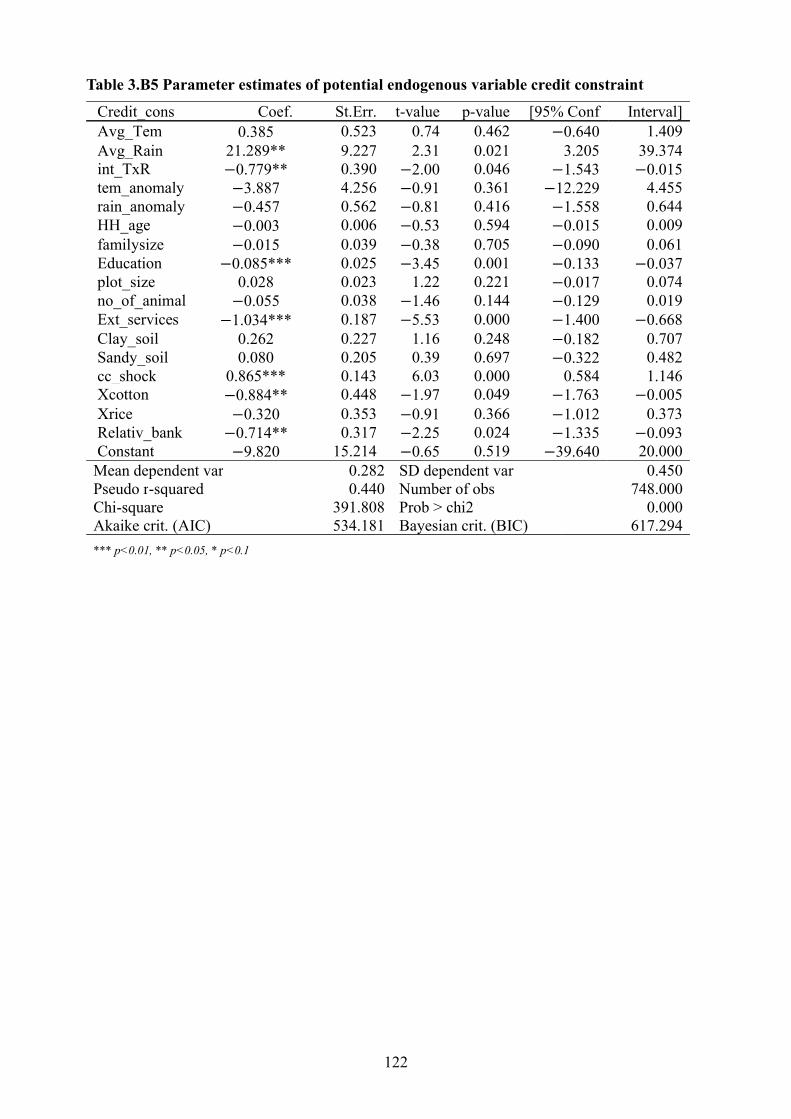
122
Table 3.B5 Parameter estimates of potential endogenous variable credit constraint
Credit_cons Coef. St.Err. t-value p-value [95% Conf Interval] Avg_Tem 0.385 0.523 0.74 0.462 −0.640 1.409 Avg_Rain 21.289** 9.227 2.31 0.021 3.205 39.374 int_TxR −0.779** 0.390 −2.00 0.046 −1.543 −0.015 tem_anomaly −3.887 4.256 −0.91 0.361 −12.229 4.455 rain_anomaly −0.457 0.562 −0.81 0.416 −1.558 0.644 HH_age −0.003 0.006 −0.53 0.594 −0.015 0.009 familysize −0.015 0.039 −0.38 0.705 −0.090 0.061 Education −0.085*** 0.025 −3.45 0.001 −0.133 −0.037 plot_size 0.028 0.023 1.22 0.221 −0.017 0.074 no_of_animal −0.055 0.038 −1.46 0.144 −0.129 0.019 Ext_services −1.034*** 0.187 −5.53 0.000 −1.400 −0.668 Clay_soil 0.262 0.227 1.16 0.248 −0.182 0.707 Sandy_soil 0.080 0.205 0.39 0.697 −0.322 0.482 cc_shock 0.865*** 0.143 6.03 0.000 0.584 1.146 Xcotton −0.884** 0.448 −1.97 0.049 −1.763 −0.005 Xrice −0.320 0.353 −0.91 0.366 −1.012 0.373 Relativ_bank −0.714** 0.317 −2.25 0.024 −1.335 −0.093 Constant −9.820 15.214 −0.65 0.519 −39.640 20.000 Mean dependent var 0.282 SD dependent var 0.450 Pseudo r-squared 0.440 Number of obs 748.000 Chi-square 391.808 Prob > chi2 0.000 Akaike crit. (AIC) 534.181 Bayesian crit. (BIC) 617.294
*** p<0.01, ** p<0.05, * p<0.1

123
Table 3.B6 Parameter estimates of of potential endogenous variable extension services
Ext_services Coef. St.Err. t-value p-value [95% Conf Interval]
CreditConstant −1.046*** 0.195 −5.36 0.000 −1.429 −0.664 Avg_Tem 0.104 0.444 0.23 0.815 −0.767 0.974 Avg_Rain 2.285 7.989 0.29 0.775 −13.373 17.944 int_TxR −0.049 0.339 −0.14 0.886 −0.713 0.616 tem_anomaly 6.120 4.318 1.42 0.156 −2.343 14.583 rain_anomaly −0.627 0.588 −1.06 0.287 −1.780 0.526 HH_age 0.005 0.005 0.99 0.324 −0.005 0.016 familysize −0.021 0.032 −0.67 0.505 −0.084 0.041 Education 0.185*** 0.021 8.82 0.000 0.144 0.226 plot_size −0.057** 0.024 −2.40 0.016 −0.103 −0.010 no_of_animal 0.020 0.034 0.58 0.563 −0.047 0.086 Clay_soil 0.133 0.177 0.75 0.452 −0.213 0.479 Sandy_soil −0.224 0.200 −1.12 0.264 −0.617 0.169 cc_shock −0.155 0.162 −0.96 0.339 −0.472 0.162 Xcotton −0.450 0.381 −1.18 0.238 −1.196 0.296 Xrice −0.397 0.316 −1.25 0.209 −1.016 0.223 dis_Ext_off −0.048** 0.021 −2.29 0.022 −0.090 −0.007 Constant −5.544 13.229 −0.42 0.675 −31.472 20.384 Mean dependent var 0.386 SD dependent var 0.487 Pseudo r-squared 0.347 Number of obs 748.000 Chi-square 346.715 Prob > chi2 0.000 Akaike crit. (AIC) 687.257 Bayesian crit. (BIC) 770.370
*** p<0.01, ** p<0.05, * p<0.1
Table 3.B7 Suest-based Hausman tests of IIA assumption
Ho: Odds (Outcome-j vs Outcome-k) are independent of other alternatives.
CSA practices Choices chi2 df P>chi2 Non-adaptation 30.704 72 1.000 Seed variety diver. 39.385 72 0.999 Cropping calendar 38.224 72 1.000 Input mix 34.986 72 1.000 SWC 42.231 72 0.998
Note: A significant test is evidence against Ho.
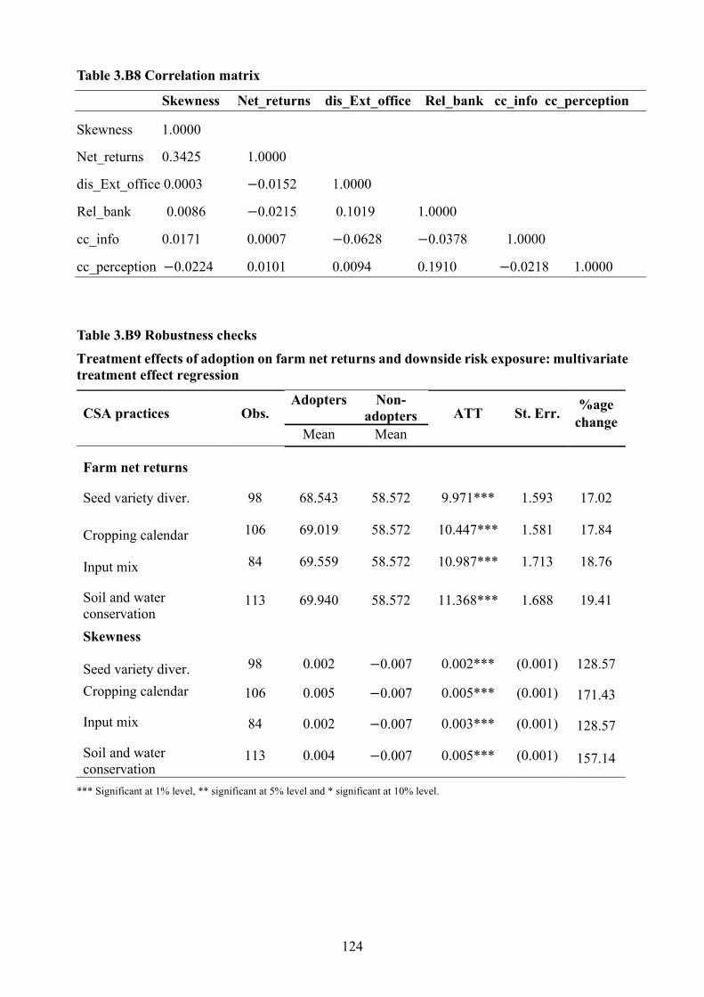
124
Table 3.B8 Correlation matrix
Skewness Net_returns dis_Ext_office Rel_bank cc_info cc_perception
Skewness 1.0000
Net_returns 0.3425 1.0000
dis_Ext_office 0.0003 −0.0152 1.0000
Rel_bank 0.0086 −0.0215 0.1019 1.0000
cc_info 0.0171 0.0007 −0.0628 −0.0378 1.0000
cc_perception −0.0224 0.0101 0.0094 0.1910 −0.0218 1.0000
Table 3.B9 Robustness checks
Treatment effects of adoption on farm net returns and downside risk exposure: multivariate treatment effect regression
CSA practices Obs. Adopters Non-
adopters ATT St. Err. %age
change Mean Mean
Farm net returns
Seed variety diver. 98 68.543 58.572 9.971*** 1.593 17.02
Cropping calendar 106 69.019 58.572 10.447*** 1.581 17.84
Input mix 84 69.559 58.572 10.987*** 1.713 18.76
Soil and water conservation
113 69.940 58.572 11.368*** 1.688 19.41
Skewness
Seed variety diver. 98 0.002 −0.007 0.002*** (0.001) 128.57
Cropping calendar 106 0.005 −0.007 0.005*** (0.001) 171.43
Input mix 84 0.002 −0.007 0.003*** (0.001) 128.57
Soil and water conservation
113 0.004 −0.007 0.005*** (0.001) 157.14
*** Significant at 1% level, ** significant at 5% level and * significant at 10% level.

125
Chapter 4
The Heterogeneous Effects of Adoption of Climate-Smart Agriculture on Household
Welfare in Pakistan
Muhammad Faisal Shahzad and Awudu Abdulai
Department of Food Economics and Consumption Studies
Published in Applied Economics (Volume 52, 2020).
Abstract
In this study, we analyze the heterogeneity in the impacts of adoption of climate-smart agricultural
(CSA) practices on welfare indicators such as food and nutrition security and poverty reduction
in Pakistan. We employ the marginal treatment effects (MTE) approach to estimate the treatment
effects heterogeneity and policy-relevant treatment effects (PRTE). The findings show substantial
heterogeneity in benefits from adoption of CSA with respect to both observed and unobserved
household characteristics. In particular, the estimates show that households with higher
unobserved benefits are more likely to adopt CSA practices. The empirical results show that
adoption of CSA practices significantly reduces household food insecurity and increases
household dietary diversity but reduces the poverty headcount and severity of poverty of the
households at the lower level of unobserved resistance to adoption. The PRTE indicate that
sources of climate change information and climate-resilient trainings could help to reduce rural
poverty and improve food and nutrition security in Pakistan.
Keywords: Climate-smart agriculture, food and nutrition security, poverty reduction, marginal
treatment effects, Pakistan.
JEL Codes: Q18, I32, Q54, C36, O33, D13.

126
4.1. Introduction
Climate change and variability continue to undermine national and global efforts to achieve
poverty reduction and food security, particularly among vulnerable populations in developing
countries. Many studies on climate change impacts indicate that rural populations in developing
countries are the most vulnerable because of their dependence on rainfed agriculture as a source
of livelihood (e.g., Barbier and Hochard, 2018; Tol, 2018). Most of these countries, which are
mainly agrarian, have adapted to changing climate to enable them feed their growing populations
to sustain livelihoods. In particular, the achievement of some of the sustainable development goals
(SDGs) that involve no poverty, zero hunger, climate action, sustainable cities, and communities,
relies heavily on fostering climate-smart food systems to feed the growing global population,
providing secure livelihoods and consuming natural resources (World Bank, 2015).
Many studies project that if no mitigation or adaptation strategies are adopted, global poverty
could increase by 35 to 122 million under climate change scenarios, mainly from decreasing
agricultural incomes and reductions in the growth of GDP (FAO, 2016). For example, Hertel et
al. (2010) report that a decrease in crop yields would lead to increases in prices of major food
staples by 10-60% in 2030. A study by Earls (2019) argues that the number of malnourished
children could increase as a result of climate change. The diverse effects of climate change, such
as increasing heat stress, decreasing cold stress, worsening drought, crops growing faster as a
result of carbon dioxide fertilization, often make it difficult to quantify the impacts (Tol, 2018).
Therefore, researchers try to focus on welfare indicators such as production efficiency, income,
poverty reduction, and food security (Khanal et al. 2018; Barbier and Hochard, 2018; Badibanga
and Ulimwengu, 2020).
The variation of climate change across the globe also implies that the impact of adaptation to
climate change and, for that matter, effects of climate-smart agricultural (CSA) practices on
welfare will vary across the globe. The FAO (2013) identified the CSA practices as the surest way
to sustainable agricultural development for food security under climate change impacts.

127
According to FAO (2013), CSA employs sustainable land management practices together with
drought-tolerant varieties with the aim of enhancing farmers’ ability to adapt to a changing
climate, as well as mitigation of greenhouse gas emissions, and sustainably increasing agricultural
productivity and food security. Despite the advantages of CSA in helping farmers adapt to the
adverse effects of climate change, there are profitable trade-offs such as slower productivity
growth and lower emissions between the goals of CSA (World Bank, 2015). To minimize these
trade-offs and to ensure positive outcomes for the three goals of food security, adaptation, and
mitigation, CSA seeks to contribute to broader development goals (Tol, 2018; World Bank, 2015;
Vale, 2016). In particular, previous literature shows that farm households have adopted different
adaptation strategies such as CSA practices, including changing input mix, change in cropping
calendar, crop diversification, crop rotation, diversifying seed varieties, soil and water
conservation, using improved seed variety, improving irrigation efficiency, and income
diversification (Abdulai, 2018; Di Falco and Veronesi, 2013; Issahaku and Abdulai, 2019). Some
of the practices mentioned above have already been employed by farmers in combination or
isolation to enhance farm production. Some studies refer to these practices as adaptation strategies
(e.g., Iqbal et al. 2015; Di Falco and Veronesi, 2013); other studies call them climate-smart
practices (e.g., Teklewold et al., 2019; Issahaku and Abdulai, 2020).
Many studies have analyzed the drivers and impacts of adoption of CSA over the past decade
(e.g., Abdulai and Huffman, 2014; Di Falco et al., 2011; Bocchiola et al., 2019; Lipper et al., 2014;
Michler et al., 2019; Mutenje et al., 2019). The impacts are normally categorized into direct and
indirect economic impacts. The direct impacts refer to the benefits attributed to the application of
specific CSA practices (such as adoption of conservation agricultural practices and drought-
tolerant varieties, etc.) at farm and household levels, while the indirect impacts include the
enhancement of carbon sinks and carbon dioxide (CO2) sequestration processes. In this study, we
focus on the direct impacts of CSA, which is on the welfare of farm households. The empirical
evidence on the direct impacts of CSA suggests that these adaptation strategies could play a crucial

128
role in the achievement of SDG’s in reducing hunger, improving food security, and conserving
natural resources (Iqbal et al. 2015; Abid et al. 2016; Ali and Erenstein, 2017; Issahaku and
Abdulai, 2019; Dakpo et al., 2019; Salim et al., 2020, etc.). A study by Issahaku and Abdulai
(2019) on Ghana concluded that adoption of CSA practices increased food and nutrition security
of smallholder farmers, while Abid et al. (2016) found that wheat productivity and crop income
increased as a result of adoption of CSA practices by farmers in Pakistan.
The studies outlined above-employed methods like propensity score matching (PSM), Heckman’s
treatment effect model or the endogenous switching regression (ESR) approaches to analyze the
impact of adoption of CSA practices on farm performance and household welfare (e.g., Ali and
Erenstein, 2017; Iqbal et al., 2015; Issahaku and Abdulai, 2020; Shahzad and Abdulai, 2020). The
shortcomings of the PSM approach has been widely documented in the literature (e.g., Di Falco
et al. 2011; Abdulai and Huffman, 2014). Heckman’s treatment effect model is estimated in two
steps, whereby a notable shortcoming of two-step estimation is that it generates the
heteroskedastic residuals that cannot be used to obtain consistent standard errors without
adjustments (Lokshin and Sajaia, 2004). Although the ESR model accounts for both observable
and unobservable factors, its critical limitation is that it accounts for selection bias by aggregating
the unobservable heterogeneity, but this heterogeneity actually varies across individuals
(Cornelissen et al., 2016).
To account for heterogeneity across households, the present study contributes to the literature by
employing the marginal treatment effects (MTE) approach to examine the drivers and impact of
adoption of CSA practices on household welfare outcomes such as food and nutrition security,
poverty, and severity of poverty using recent data from 540 farmers from Pakistan. We use
household dietary diversity score (HDDS) and household food insecurity access scale (HFIAS) to
capture food and nutrition security (Swindale and Bilinsky, 2006; Coates et al., 2007), and then
the poverty headcount and poverty gap to measure the poverty status of farm households. The
MTE approach takes into account both observable and unobservable factors influencing adoption

129
of CSA practices based on propensity scores and draws the MTE curve against varying levels of
unobservable resistance to CSA adoption. The approach further allows us to estimate the
treatment effect heterogeneities, and also simulate the effects of policy changes on the welfare
indicators.
The rest of the paper is structured as follows. The next section presents the conceptual framework
and empirical specification. In section 4.3, we discuss the data and descriptive statistics. Section
4.4 presents the empirical results, while the final section concludes with policy implications.
4.2. Conceptual framework and estimation
In this section, we present a simple framework to illustrate how adoption decisions of farm
households impact on welfare. We assume that in the decisions to adopt CSA practices, farmers
consider the potential net benefits from adoption. Thus, if the potential benefits of adopting CSA
practices are greater than the benefits of non-adoption, farmers tend to adopt. The adoption
decision is expected to impact welfare outcomes such as food and nutrition security measures and
poverty status of households.
Consider 𝑦 to be the outcome variables such as household dietary diversity score (HDDS),
household food insecurity access scale (HFIAS), poverty headcount index and poverty gap index,
and 𝐴 as the adoption status of the 𝑖th farmer, where 𝐴 takes the value of one in case the farmer
adopts CSA practices, and zero otherwise. The empirical relationship between outcome variables
and adoption is specified as follows:
𝑦 = 𝛽 𝑋 + 𝜃𝐿 + 𝑢 , 𝑗 = 0, 1. (4.1)
where 𝑋 is a vector of household and farm level controls such as household characteristics (age
education, dependency ratio), the ownership of assets (such as ownership of animals), past
climatic factors (e.g., average daily temperature, average daily rainfall, temperature anomaly,
rainfall anomaly, and their interactions), off-farm income, past experience of extreme weather
events captured as past climate shocks, access to extension services, credit constraints, and soil

130
characteristics (soil types). 𝐿 captures location fixed effects, 𝛽 and 𝜃 are the parameters to be
estimated, and 𝑢 represents derivations from the mean, assumed to have zero mean and constant
variance. For simplicity, we drop 𝐿 from the further derivation of equations. The 𝑗 subscript
denotes adoption status where 𝑗 = 1 represents adopter, and 𝑗 = 0 represents non-adopter.
As indicated above, farmer 𝑖 will adopt CSA practices, if the expected gains from adoption (𝑦 )
are higher than the gains from non-adoption (𝑦 ). Let 𝐴 ∗ be the expected net gains from adoption,
then 𝐴 = 1, if 𝐴 ∗ = 𝑦 − 𝑦 ≥ 0, otherwise 𝐴 = 0 . 𝐴 ∗ is the latent propensity to adopt. To
the extent that adoption of CSA practices is non-random, as farmers self-select into adoption based
on observable and unobservable characteristics, the decision to adopt is endogenous. The latent
variable 𝐴 ∗ cannot be directly measured but can be specified as a function of observable
characteristics. We can thus model farmers adoption decisions as follows:
𝐴∗ = 𝑓 (𝑋 , 𝑍 ) − 𝑉 (4.2)
where 𝐴∗ is the latent variable that captures the expected gains from adoption, 𝑍 represents
excluded instruments used for identification of the model, and 𝑉 measures the unobserved
heterogeneity in the propensity to adopt. The negative sign in Eq. (4.2) shows that unobserved
resistance restricts farmers from adopting CSA practices. Following Cornelissen et al. (2018), the
transformation of the selection rule in Eq. (4.2) can be specified as:
𝑓 (𝑋 , 𝑍 ) − 𝑉 ≥ 0 ⇔ 𝑓 (𝑋 , 𝑍 ) ≥ 𝑉 ⇔ 𝑔 [𝑓 (𝑋 , 𝑍 )] ≥ 𝑔 (𝑉 ),
where 𝑔 denotes the cumulative distribution function of 𝑉 (in our case, standard normal
distribution). The term 𝑔 [𝑓 (𝑋 , 𝑍 )] , also denoted by 𝑔 [𝑓 (𝑋 , 𝑍 )] ≡ 𝑃(𝑋 , 𝑍 ) is the
propensity score (the probability that farmer i with observed characteristics 𝑋 , and excluded
instruments 𝑍 will adopt CSA practices), and 𝑔 (𝑉 ) denoted by 𝑔 (𝑉 ) ≡ 𝑈 represents the
quantiles of the distribution of unobserved resistance to adoption (𝑉 ). Given the potential outcome
specification in Eq. (4.1), and the adoption decisions in Eq. (4.2), heterogenous expected gains
conditional on observed and unobserved characteristics of farmers can be specified as follows:
131
𝑌 = 𝐴 𝑦 + (1 − 𝐴 )𝑦 = 𝑦 + 𝐴 (𝑦 − 𝑦 ) = 𝑋 𝛽 + 𝐴 [𝑋 (𝛽 − 𝛽 )+𝑈 − 𝑈 ]≡∆
+ 𝑈
(4.3)
here ∆ ≡ 𝑦 − 𝑦 = 𝑋 (𝛽 − 𝛽 )+𝑈 − 𝑈
To identify the parameters of the model in Eqs. (4.2) and (4.3), the standard instrumental variable
(IV) assumptions should be satisfied. In particular, the conditional independence (exclusion
restriction) assumption that (𝑈 , 𝑈 , 𝑈 ) is statistically independent of 𝑍 , given 𝑋 , needs to be
satisfied.
In the analysis, we use the number of climate-information sources from which a farm household
obtains information related to climate change and the number of climate-resilient trainings
attended as excluded instruments. Climate change tends to positively influence innovation
processes through information sources and training (Hakimi and Inglesi-Lotz, 2020; Véganzonès-
Varoudakis, and Plane, 2019). These climate-information sources such as agricultural extension,
print media, past weather records, television (TV), information and communication technology
(ICT), and personal exchange with neighboring farmers positively influence innovation processes
and are good predictors of adoption decisions of farmers (Di Falco et al., 2011; Lu, 2011). These
sources enable farmers to obtain information about the prevailing weather trends and the expected
weather changes. Similarly, climate-resilient trainings help farmers to understand the effects of
climate change and the various adaptation measures available to farmers (Aryal et al., 2018). It is
important to note that these climate-resilient preparations may be endogenous if trainers focus on
a specific group of adopters of CSA practices, or adopters of particular practices interested in
getting these trainings that may affect the outcomes. However, our survey shows that all farmers
had equal chances of participating in these trainings, irrespective of specific adopter groups or
practices. Further to check internal validity of these two instrumental variables, we conducted
several statistical tests. The Wald test for the joint significance of these instruments at the first
stage probit estimation shows that the instruments jointly and significantly influence adoption of

132
CSA practices, while simple OLS regression for outcome equations of these variables is
insignificant for non-adopters. A further test of correlation confirmed that these instruments are
uncorrelated with outcome variables, indicating the validity of the excluded instruments.13
Following Eq. (4.3), the marginal treatment effects can be defined as a function of the quantiles,
or the treatment effect at a particular value of 𝑈 (Cornelissen et al., 2016).
MTE (𝑋 = 𝑥, 𝑈 = 𝑢 ) = 𝐸[∆ |𝑋 = 𝑥, 𝑈 = 𝑢 ] (4.4a)
The treatment effect for an individual with observed characteristics 𝑋 = 𝑥 who are at 𝑢 -th
quantile of the V distribution will have a propensity score 𝑃(𝑋 , 𝑍 ) = 𝑢 . This implies that such
a farmer is indifferent to adoption. Now invoking the assumption that MTE is additively separable
into observable and unobservable components, it can be expressed as:
MTE(𝑥, 𝑢 ) = 𝐸(∆ |𝑋 = 𝑥, 𝑈 = 𝑢 )
= 𝑥(𝛽 − 𝛽 )𝒐𝒃𝒔𝒆𝒓𝒗𝒆𝒅 𝒄𝒐𝒎𝒑𝒐𝒏𝒆𝒏𝒕
+ 𝐸(𝑈 − 𝑈 |𝑈 = 𝑢 )𝒖𝒏𝒐𝒃𝒔𝒆𝒓𝒗𝒆𝒅 𝒄𝒐𝒎𝒑𝒐𝒏𝒆𝒏𝒕
(4.4b)
Given Eq. (4.3) and the propensity score, the outcome equation can be estimated as a function of
the observed characteristics as defined above, and the propensity score as:
E(𝑌 |𝑋 = 𝑥, 𝑃(𝑋 , 𝑍 ) = 𝑝) = 𝑋 𝛽 + 𝑋 ( 𝛽 − 𝛽 )𝑝 + 𝐾(𝑝) (4.5)
where 𝑌 measures the returns to adoption for households with different levels of observable
characteristics, 𝑋 = 𝑥, the propensity score 𝑝, and 𝐾(𝑝) is a nonlinear function of the propensity
score.
Taking the derivative of Eq. (4.5) with respect to 𝑝 delivers the MTE (Heckman and Vytlacil 2005;
Carneiro et al., 2017; Cornelissen et al., 2016) as:
13 In OLS estimates of outcome variables for non-adopters, the F-test shows that the instruments are not jointly statistically significant (see Table 4.C1-4.C4 in Appendix C). For correlation test see Table 4.C5 in Appendix C.

133
MTE (𝑋 = 𝑥, 𝑈 = 𝑝) = ( | , ( , ) )
= 𝑥( 𝛽 − 𝛽 ) +( )
(4.6)
We estimate the treatment effects by first estimating the selection Eq. (4.2) as a probit model to
obtain estimates of 𝑃(𝑋 , 𝑍 ) as �̂�, and in the second stage, we estimate the outcome equations as:
𝑌 = 𝑋 𝛽 + 𝑋 ( 𝛽 − 𝛽 )�̂� + ∑ 𝛼 �̂� + 𝜉 (4.7)
We derive the MTE curve from Eq. (4.7) by taking the derivative with respect to �̂�. We assume a
second-order polynomial in �̂� (i.e., 𝑘 = 2 ) in our baseline specification. To ascertain the
sensitivity of the MTE curve to the functional form assumed, we also estimate MTE curves as
robustness checks by using 𝑘 = 1, 𝑘 = 3, 𝑘 = 4. As shown in Heckman and Vytlacil (2005), the
MTE can be aggregated over 𝑈 in different ways to obtain average treatment effects (ATE),
average treatment effects on the treated (ATT), average treatment effects on the untreated (ATU),
and local average treatment effects (LATE). 14 Thus, different other parameters of interest can be
estimated as the weighted averages of the MTE. To the extent that we are also interested in the
impact of policy intervention on the returns to adoption, we use the policy-relevant treatment
effects (PRTE) to simulate baseline and alternate policies as follows:
𝑃𝑅𝑇𝐸(𝑋) = [ | , ] [ | , ]
[ | , ] [ | , ] (4.8)
The PRTE measures the average returns to adoption for a farmer who is induced to change his
adoption decision in response to specific policies. In the present study, the policy variables include
climate information sources and climate-resilient trainings.
14 In the interest of brevity, the equations to calculate ATE, ATT, ATU, and LATE are given below: ATE = 𝐸[𝑦 − 𝑦 ] = 𝐸[𝛽 (𝑋 ) − 𝛽 (𝑋 )] (a) ATT = 𝐸[𝑦 − 𝑦 |𝐴 = 1] + 𝐸[𝑈 − 𝑈 |𝐴 = 1] = 𝐸[𝛽 (𝑋 ) − 𝛽 (𝑋 )|𝐴 = 1] + 𝐸[𝑈 − 𝑈 |𝐴 = 1] (b) ATU = 𝐸[𝑦 − 𝑦 |𝐴 = 0] + 𝐸[𝑈 − 𝑈 |𝐴 = 0] = 𝐸[𝛽 (𝑋 ) − 𝛽 (𝑋 )|𝐴 = 0] + 𝐸[𝑈 − 𝑈 |𝐴 = 0] (c) 𝐿𝐴𝑇𝐸 = 𝐸[𝑦 − 𝑦 |𝐴 > 𝐴 , 𝑋 = 𝑥] = 𝛽 (𝑋 ) − 𝛽 (𝑋 ) + 𝐸[𝑈 − 𝑈 |𝐴 > 𝐴 , 𝑋 = 𝑥] (d)
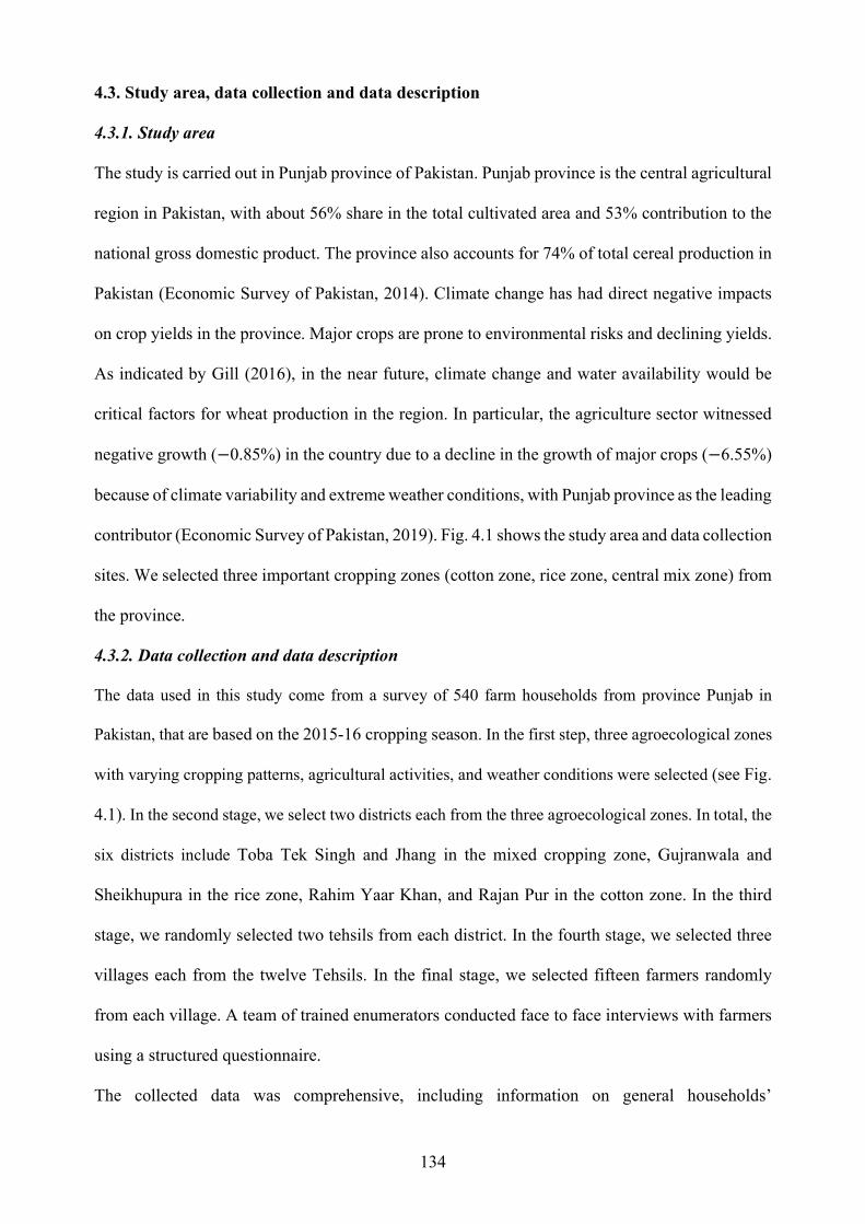
134
4.3. Study area, data collection and data description
4.3.1. Study area
The study is carried out in Punjab province of Pakistan. Punjab province is the central agricultural
region in Pakistan, with about 56% share in the total cultivated area and 53% contribution to the
national gross domestic product. The province also accounts for 74% of total cereal production in
Pakistan (Economic Survey of Pakistan, 2014). Climate change has had direct negative impacts
on crop yields in the province. Major crops are prone to environmental risks and declining yields.
As indicated by Gill (2016), in the near future, climate change and water availability would be
critical factors for wheat production in the region. In particular, the agriculture sector witnessed
negative growth (−0.85%) in the country due to a decline in the growth of major crops (−6.55%)
because of climate variability and extreme weather conditions, with Punjab province as the leading
contributor (Economic Survey of Pakistan, 2019). Fig. 4.1 shows the study area and data collection
sites. We selected three important cropping zones (cotton zone, rice zone, central mix zone) from
the province.
4.3.2. Data collection and data description
The data used in this study come from a survey of 540 farm households from province Punjab in
Pakistan, that are based on the 2015-16 cropping season. In the first step, three agroecological zones
with varying cropping patterns, agricultural activities, and weather conditions were selected (see Fig.
4.1). In the second stage, we select two districts each from the three agroecological zones. In total, the
six districts include Toba Tek Singh and Jhang in the mixed cropping zone, Gujranwala and
Sheikhupura in the rice zone, Rahim Yaar Khan, and Rajan Pur in the cotton zone. In the third
stage, we randomly selected two tehsils from each district. In the fourth stage, we selected three
villages each from the twelve Tehsils. In the final stage, we selected fifteen farmers randomly
from each village. A team of trained enumerators conducted face to face interviews with farmers
using a structured questionnaire.
The collected data was comprehensive, including information on general households’

135
characteristics, landholding, agronomic practices, production and costs, types of crops cultivated,
irrigation water use, access to extension, responses to climate change, access to credit, farm, and
household assets, off-farm income sources, consumption, and expenditure. One section of the
questionnaire was mainly designed to capture climate change perceptions, information, and
climate risks in order to understand adaptation responses to climate change. Farmers were also
asked if they had taken climate-resilient training in the past, as well as the number of sources they
got information related to climate change. Most of the adopters were very well informed about
climate change, but few farmers attended climate-resilient trainings, because there was no well-
organized program from the government to support climate-resilient trainings. In line with
previous adoption studies, we also captured plot-level characteristics such as soil types.
Fig. 4.1 Map of Pakistan showing study area and data collection sites
Information was also gathered on the adaptation strategies, specifically on climate-smart
agricultural (CSA) practices. The main CSA practices include change in cropping calendar,

136
diversified seed varieties, changing input mix, and soil and water conservation measures. Evidence
from our data shows that farmers adopt CSA practices, such as changing cropping calendar, soil
and water conservation measures, diversifying seed variety, and changing input mix to cope with
climate change and variability. Soil and water conservation measures employed include soil
erosion control measures, such as soil bunds and crop rotation to conserve soil moisture and
prevent nutrient loss in the soil, as well as cover crops to fix nitrogen in the soil. Diversification
of seed varieties includes the use of drought-resistant and early maturing varieties that enable
farmers to cope with erratic rainfall or very low rainfall. Changing input mix includes the changing
fertilizer and application method, change in pesticide use, changing the use of herbicides or
weedicides, and micro-nutrients.
Two sub-sections were specially developed to ask questions related to food and nutrition security.
The food security access scale (HFIAS) and the household dietary diversity score (HDDS) are the
two indicators used to measure food and nutrition security. The HSIAS is a scale that captures the
psychological and behavioral dimensions of food insecurity in terms of access to food (Coates et
al. 2007; Maxwell et al., 2014). The scale ranges between 0 and 27, with zero scores representing
a household with no reported food insecurity. The maximum value of 27 represents the highest
level of food insecurity, with high frequency of consuming less food and skipping meals due to
insufficient access to food (Coates et al. 2007). For HDDS, following Swindale and Bilisnky
(2006), we used seven days recall period, asking households on food consumed during the last
seven days. The food items were divided into twelve food groups; cereals, tubers and roots,
vegetables, fruits, meat and poultry, eggs, fish, pulses and nuts, legumes, milk and milk products,
oils and fats, sugar and honey, and miscellaneous. Further, these groups were assigned numerical
values (1 to 12) that were used to calculate the HDDS, which is a good predictor of dietary
diversity at the household level. To measure poverty, we use the poverty headcount index and

137
poverty gap index (Foster et al., 1984).15
Secondary information related to temperature and rainfall was collected from the National Center
for Environmental Prediction (NCEP) and World Weather Online. The collected information
ranges from 1979 to 2016 up to the same year in which we obtained data from farmers. It was
converted from monthly to yearly averages. As the Punjab province is mostly flat, we used the
inverse distance method of spatial interpolation to calculate location-specific farm-level
temperature and rainfall. For this purpose, we used the global positioning system (GPS) to record
the farm location (elevation, longitude, and latitude) during the data collection. The recorded farm
locations were employed to interpolate information on farm-level temperature and rainfall.
Subsequently, we calculated the temperature and rainfall anomalies taking 2016 as a base year in
which we collected primary data from farmers. We use binary variable for adopters and non-
adopters; farmers who practice one or more CSA practices at the farm are considered adopters and
assigned a value of one. In contrast, farmers who did not practice any of the CSA practices are
categorized as non-adopters and assigned zero value.
Table 4.1 shows definitions and descriptive statistics of selected variables. On average, we find
that 48% of farmers are adopters of CSA practices, with the remaining 52% classified as non-
adopters in the sample. On average, farm households’ food insecurity access scale is 7.36, with a
dietary diversity score of 7.49. The estimated average headcount index shows that about 24% of
farm households are below the poverty line, and do not have enough financial resources (dollar
15 We used the Foster–Greer–Thorbecke (FGT) (1984) indices to estimate poverty in our data sample by using the formula: 𝐹𝐺𝑇 =
∑ , where 𝛾 = 0, 1. When 𝛾 = 0 then 𝐹𝐺𝑇 = and for 𝛾 = 1, 𝐹𝐺𝑇 = ∑ . where 𝑁 is the total number
of people in a household, 𝑃𝐿 represents the poverty line, ℎ represents per capita income of the ith person in a household, and 𝛾 represents the poverty aversion parameter. When 𝛾 = 0, 𝐹𝐺𝑇 is simply the headcount index or the proportion of people that are poor. When 𝛾 = 1, 𝐹𝐺𝑇 is the poverty gap index, which reflects the severity or intensity of poverty defined by the mean distance to the poverty line. Thus, the poverty gap index, which captures the severity of poverty, is the average shortfall in income for the farm household, from the poverty line. Hence, 𝐹𝐺𝑇 represents the severity of poverty and reflects the extent of inequality among the poor households.

138
1.90 a day) for the minimum standard of living.16 The estimated poverty gap index is about 35%,
indicating that the average shortfall in income from the poverty line for the sample is 35%.
Table 4.2 displays the mean differences in the characteristics of adopters and non-adopters. It is
evident from the table that there are some statistically significant differences between adopters
and non-adopters of CSA practices with respect to household and farm level characteristics. There
appear to be differences in access to credit and farm sizes. On average, adopters cultivate 6 acres
more land than non-adopters and are less credit constrained. The average 10 % of adopters are
liquidity constraint, as much as 37% of non-adopters are credit constrained. There are also
differences in terms of schooling year and access to extension services, adopters are more educated
and have frequent contacts with extension agents compared with non-adopters. Adopters are also
different than non-adopters in terms of climate knowledge acquisition. On average, adopters
access at least one information source to acquire climate change information compared with non-
adopters’ 0.14 climate information sources. Adopters attend higher climate-resilient trainings than
non-adopters. These simple comparisons also reveal that adopters are less food insecure, have
higher dietary diversity, and experience lower levels of poverty as well as the severity of poverty.
In particular, the average HFIAS of an adopter household is less than that of non-adopter
household, indicating that the adoption of CSA practices plays a significant role in decreasing
farm households’ food insecurity. Similarly, the average HDDS is higher than that of non-
adopters’ HDDS, suggesting that adoption of CSA practices increases household dietary diversity.
Adopters and non-adopters also appear to exhibit different poverty status. On average, 12%
adopters of CSA practices are poor, while as much as 56% of non-adopters fall below the poverty
line, indicating that adoption of CSA practices significantly reduces poverty of farm households.
There is also a difference between adopters and non-adopters in terms of the poverty gap; the
16 We used international poverty line (dollar 1.90 a day) indicated by the World Bank to calculate poverty headcount and poverty gap indices of farm households.

139
average the shortfall of adopters from the poverty line is 5%, while the shortfall for non-adopters
is 41%, which means that adoption reduces poverty severity.
Table 4.1 Descriptive Statistics and definition of selected variables
Variables Definitions Mean Std. Dev.
CC_adoption 1 if farmer adapts to climate change, 0 otherwise 0.485 0.500
HFIAS_score Household food insecurity access score (0-27 scale), where 0 represents that household is food secure, while 27 represents that household is food insecure
7.363 7.565
HDDS Household dietary diversity score (0-12 scale), where 0 represents no diversity in food while 12 represents perfect food diversity in a household
7.491 2.722
Poverty_HC 1 if a household is living below the poverty line, 0 otherwise 0.235 0.419
Poverty_gap Mean distance of poor household from the poverty line 0.346 0.476
Credit_const 1 if household is credit constrained, 0 otherwise 0.235 0.425
Avg_Tem Average daily temperature in (Degrees Celsius) 27.328 1.129
Avg_Rain Average daily rainfall (millimeters) 0.648 0.559
Int_TxR Product of average temperature and average rainfall (number) 17.119 13.976
Tem_anomaly Change in temperature relative to baselinea (number) 0.215 0.032
Rain_anomaly Change in rainfall relative to baseline (number) −0.372 0.192
Int_TxR Product of temperature anomaly and rain anomaly (number) −0.083 0.049
Off_farm Farmer’s income other than agricultural activities (000 dollars) 0.701 1.805
HH_age Household head age (years) 47.009 11.382
Dep_ratio Ratio off non-earning individuals to the earning individuals 4.420 1.723
Education Number of schooling years household head completed (years) 6.431 4.495
Farm_size Total number of acres farm household cultivate (acresb) 9.403 9.138
Herd size Number of animals a farm household owns (number) 3.483 1.930
Ext_services 1 if farmer has contact with extension agent, 0 otherwise 0.572 0.495
CC_shock 1 if farmer faced climate shock in the past three years, 0 otherwise 0.254 0.436
Rice zone 1 if farmer resides in rice growing zone, 0 otherwise 0.333 0.472
Cotton zone 1 if farmer resides in cotton growing zone, 0 otherwise 0.331 0.471
Clay_soil 1 if the soil at farm is clay loam, 0 otherwise 0.161 0.368
Sandy_soil 1 if the soil at farm is sandy loam, 0 otherwise 0.135 0.342
info_sources Number of sources from which a farmer obtains information related to sustainable agricultural practices (number)
0.526 0.607
CR_trainings Number of training days a farmer attends on CSA practices (number)
0.331 0.699
No. of obs. 540
a Anomaly= (current year mean -long term mean)/long term mean
b 1 acre= 0.40 hectare

140
Table 4.2 Descriptive statistics and mean difference between adopters and non-adopters
Variables Adopters Non_adopters Mean difference Std. Errors HFIAS_score 3.279 13.212 −9.934*** 0.586 HDDS 8.736 6.316 2.420*** 0.210 Poverty_HC 0.122 0.555 −0.434*** 0.036 Poverty_gap 0.049 0.411 −0.362*** 0.033 Credit_const 0.096 0.367 −0.272*** 0.035 Avg_Tem 27.404 27.256 0.147 0.097 Avg_Rain 0.613 0.682 −0.070 0.048 Int_TxR 16.217 17.968 −1.752 1.202 Tem_anomaly 0.219 0.212 0.006** 0.003 Rain_anomaly −0.379 −0.366 −0.012 0.017 Int_anom_TXR −0.086 −0.080 −0.005 0.004 Off_farm 0.798 0.610 0.189 0.156 HH_age 48.481 45.623 2.858*** 0.973 Dep_ratio 4.680 4.176 0.503*** 0.147 Education 7.199 5.708 1.490*** 0.382 Farm_size 12.972 6.040 6.931*** 0.729 Herd size 4.194 2.813 1.382*** 0.156 Ext_services 0.848 0.313 0.534*** 0.036 CC_shock 0.462 0.058 0.405*** 0.033 Xrice 0.344 0.324 0.020 0.041 Xcotton 0.309 0.352 −0.043 0.041 Clay_soil 0.145 0.176 −0.031 0.032 Sandy_soil 0.084 0.184 −0.100*** 0.029 info_sources 0.931 0.144 0.787*** 0.040 CR_trainings 0.626 0.054 0.572*** 0.055 No of Obs. 262 278 -- --
*** Significant at 1% level, ** significant at 5% level and * significant at 10% level.
These differences in averages of outcomes between adopters and non-adopters provide some
useful information in terms of the positive impact of adoption. However, this comparison of
average differences does not account for confounding factors such as observable and unobservable
farm and household characteristics. We, therefore, use the marginal treatment effect (MTE) model
to account for confounding factors, selection bias, and potential heterogeneity in impacts.
4.4. Results and discussion
In this section, we present the results from the empirical analysis. First, we discuss the estimates
of the selection equation, which reveals the drivers of adoption of CSA practices. We then present
the results of the second-stage estimation showing the impact of adoption on the outcome

141
variables. Finally, we outline the results of the PRTE. We report bootstrapped standard errors
throughout the results, with clustering at the zonal level.
4.4.1. First stage (selection equation) results
Tables 4.3-4.6 displays the first-stage parameter estimates of the probit selection equation in the
first columns. As indicated previously, we use climate-resilient trainings and the number of
information sources as identifying instruments for our estimations. We test the joint significance
of excluded instruments in the outcome equations by using a Wald test. The value of the Wald
statistics (108.18) is highly significant (at the 1% level), indicating that the instrumental variables
highly influence adoption decisions. To test the validity of the selection instruments, we also
perform F-test, which shows that the instruments do not influence the outcome variables,
signifying the validity of the excluded instruments from outcome equations.17 As we used the same
variables to analyze all dependent variables, the results from the first-stage probit model are
similar for all the specifications. Hence, we interpret the first columns’ results of the Tables 4.3-
4.6 together. Here, it is significant to explain the results shown in Fig. 4.2, exhibiting common
support. Fig. 4.2 plots the frequency distribution of the propensity score by adoption status. The
propensity scores are predicted from the baseline first stage probit regression in columns 1 of
Tables 4.3-4.6. It is evident from Fig. 4.2 that the first-stage regression produces common support
that ranges from 0.02 to 0.99. It shows the unconditional common support that is generated by
variation in both the instruments and covariates in the second stage. This satisfies the assumption
generally made in MTE applications that the shape of the MTE curve does not vary with control
variables (Cornelissen et al., 2018).
From the first columns of Tables 4.3-4.6, it is clear that climate-resilient training, as well as using
several climate information sources, are strong predictors of adoption of CSA practices, as
17 In the interest of brevity, the empirical results are reported in Appendix C (see Table 4.C1-4.C4).

142
expected. The coefficient of the variable representing climate change information sources is
positive (1.879) and significant (at the 1% level), indicating that obtaining climate change
information from different sources increases the likelihood of adoption. Similarly, a positive
(0.836) and significant (at the 1% level) coefficient of climate-resilient training suggests that
farmers who get climate-resilient training are more likely to adopt CSA practices. However, the
coefficient of the variable representing credit constraints is negative and significant, suggesting
that farmers who are credit-constrained are less likely to adopt CSA practices. This finding is
similar to the results reported by Teklewold et al. (2019b), that credit-constrained farmers find it
difficult to purchase farm inputs required for CSA practices, and therefore are less likely to adopt
these practices.
Fig. 4.2 Common support
(Frequency distribution of the propensity score by adoption status)
01
02
03
04
0D
ensi
ty
0 .2 .4 .6 .8 1Propensity score
Treated Untreated
Common support

143
We use average daily temperature, average daily rainfall, temperature anomaly, rainfall anomaly,
as well as interactions of these variables calculated at household level to capture the impact of
these climate variables on adoption decisions. The coefficient of average daily rainfall is negative
and significant, suggesting that average daily rainfall negatively and significantly affects adoption
decisions. In Pakistan, average daily rainfall is generally low (0.65 mm, see Table 4.1), hence with
increasing rainfall, farmers become less likely to invest in irrigation, which is an adaptation
strategy. Although the coefficient of average daily temperature is positive, it is not statistically
significant. Also, temperature and rainfall appear to be inversely related, higher rains associated
with lower temperatures and vice versa (Deressa et al., 2011). To account for the cumulative effect
of average daily temperature and rainfall, we use an interaction term as a product of these two
variables. The coefficient of this interaction term is positive (2.380) and statistically significant
(at the 5% level), indicating that if average daily rainfall remains constant, increasing average
daily temperature has a positive impact on adoption of CSA practices. The coefficient of rainfall
anomaly is positive and significant at the 5% level, suggesting that rainfall anomaly positively
influences adoption. As rainfall anomaly shows negative shocks in the study area and depending
on the water requirements of the crop, farmers adapt to these adverse shocks by implementing soil
and water conservation schemes, which result in rainfall anomaly having a positive impact on
adoption. On the other hand, temperature anomaly has a negative and statistically significant effect
on adoption. To consider the cumulative impact of temperature and rainfall anomalies, we
incorporated the product of these two variables as an interaction term into our analysis. The
coefficient of these anomalies’ interaction term is negative and statistically significant, showing
that if rainfall anomaly remains constant, then temperature anomaly negatively influences
adoption decisions.
The negative albeit statistically insignificant coefficient of off-farm income suggests that
households participating in off-farm work are less likely to adopt CSA practices, a result that is in
contrast to the study by Oseni and Winters (2009), who found that income from off-farm work

144
increases the likelihood of adoption due to the income effect. It is important to note that farmers
who take part in off-farm work have to reduce the time allocated to on-farm practices, referred to
as lost-labor effect. In our case, this lost-labor effect dominates the income effect, a finding that
is consistent with Kousar and Abdulai (2016) for Pakistan, who found that inorganic fertilizer use
declined with participation in off-farm work, supporting the notion of lost-labor effect on input
use. The coefficient of the variable representing education is positive and statistically significant,
highlighting the positive influence of human capital on adoption, a finding that is in line with the
previous studies (e.g., Huffman, 2020). The coefficient of the variable representing extension
services is positive and significant, indicating that the farmers who have frequent contacts with
extension agents are more likely to adopt CSA practices. Previous studies also confirmed the
positive and significant effect of extension contacts on adoption (e.g., Wossen et al., 2017; Di
Falco et al., 2011). The coefficient of the variable climate-related shocks is positive (1.434) and
significant at the 1% level, indicating that farmers who have already experienced climate-related
shocks in the past are more likely to adopt CSA practices.
4.4.2. Second stage estimation
In this subsection, we report results from the second-stage estimation based on Eq. (4.7), in
columns 2 and 3 of Tables 4.3-4.6, for the effect of the climate change variables and other controls
as well as the treatment effects of these variables on the outcome variables. The results point to
an equalizing effect of adoption on the outcome variables with different observed characteristics.
The untreated state (𝛽 ) is given in column 2, while the treated or adoption state (𝛽 − 𝛽 , which
refer to gains from CSA adoption) is given in column 3 of each table. In next sub-sections, we will
explain MTE curves shown in figures 4.3-4.6, that display MTE curves at the mean values of our
observed characteristics (𝑋 ), and relate the unobserved components of outcomes (𝑈 − 𝑈 ), and
the unobserved components of adoption choice (𝑈 ). We also specify different functional forms
of the MTE curve to check the sensitivity of the curve to such functional forms as robustness
checks.

145
Household food insecurity access scale (HFIAS)
Table 4.3 displays estimates from the untreated state in column 2 and the treatment effects in
column 3 to show the effect of adoption on the impacts of these variables on household food
insecurity access scale (HFIAS). The positive and significant coefficient of the credit constraints
variable at the untreated state, suggest that credit-constrained households are more likely to be
food insecure by about 11 points on the household food insecurity access scale. However, when
credit-constrained farmers adopt CSA practices, they are likely to reduce food insecurity by 8
points (see credit constraint in column 3 of Table 4.3, which refers to 𝛽 − 𝛽 in Eq. 4.7).
Similarly, the coefficient of the variable dependency ratio is positive and significant at the
untreated (non-adaptation) state, suggesting that households with high dependency ratios are more
food insecure, but adoption of CSA practices tend to improve their food security by 1.38 points.
The negative and significant coefficient of farm size at the untreated state indicates that larger
farm size tends to reduce household food insecurity. However, the positive and statistically
significant coefficient in the adoption state indicates that households with smaller farm sizes tend
to almost catch up with households having larger farm sizes by reducing food insecurity by about
0.463 points when they adopt. The negative and significant coefficient of extension services
variable indicates that extension contacts reduce food insecurity at the non-adoption state;
however, gains after adoption are not significant, although positive, which suggests that farmers
without extension contact may benefit more from adoption.

146
Table 4.3 Selection equation and outcome equations results for HFIAS
Note: Bootstrapped standard errors are reported with 500 replications.
*** Significant at 1% level, ** significant at 5% level and * significant at 10% level.
Variables Selection Outcome (𝜷𝟎) Outcome (𝜷𝟏 − 𝜷𝟎)
Coef. St. Err. Coef. St. Err. Coef. St. Err.
Constant −40.749 29.296 −22.633 74.747 −9.823 78.335
Credit_const −1.240** 0.610 11.604*** 2.223 8.084** 3.593
Avg_Tem 1.555 1.073 0.604 2.718 0.549 2.692
Avg_Rain −56.227** 26.893 50.152 74.518 −40.915 83.819
Int_TxR 2.380** 1.131 −1.952 3.112 1.622 3.450
Tem_anomaly −43.901* 25.302 69.353 75.083 −38.371 93.062
Rain_anomaly 24.575** 11.503 −25.733 34.286 8.023 38.239
Anom_TxR −120.394** 54.508 141.131 157.540 −51.222 173.606
Off_farm_inc −0.152 0.188 0.188 0.889 1.915* 1.018
HH_age 0.010 0.008 0.003 0.036 −0.009 0.050
Dep_ratio 0.022 0.079 1.587*** 0.420 −1.384*** 0.517
Education 0.140* 0.072 −0.099 0.364 −0.367 0.426
Farm_size 0.016 0.017 −0.549*** 0.119 0.463*** 0.134
Herd size 0.001 0.087 0.782 0.509 −0.295 0.623
Ext_services 0.966** 0.462 −3.577** 1.685 0.077 3.797
CC_shock 1.434*** 0.269 −1.336 2.212 0.934 2.414
Clay_soil −0.912** 0.360 −2.311* 1.308 1.240 1.686
Sandy_soil 0.456 0.373 0.396 1.182 −2.257 1.624
Xrice −0.203 0.812 −0.826 1.393
Xcotton −2.020** 0.896 0.538 1.711
Info_sources 1.879*** 0.193
CR_Trainings 0.836*** 0.174
𝜒 for test of excluded instruments 108.18
p-value for test of excluded instruments 0.000
p-value for test of observed heterogeneity 0.000
Observations 540

147
Household dietary diversity score (HDDS)
Table 4.4 presents the second-stage estimations for household dietary diversity scores (HDDS) at
the non-adoption state in column 2 and gains from adoption in column 3. The coefficient of the
credit constraints variable is negative and statistically significant at the non-adoption state,
indicating that credit-constrained households have lower levels of food security. The coefficient
of the off-farm income is negative and significant at the treatment state, indicating that
participating in off-farm work negatively affects gains from adoption. As mentioned earlier, the
lost labor effect dominates the income effect of participation in off-farm work. Thus, labor is
invested in off-farm work at the expense of farm activities. However, the additional income from
off-farm work is not used to improve household nutrition security. Also, farmers with higher off-
farm income are less likely to adopt and these are those with higher dietary diversity in the non-
adoption state. This implies households with lower off-farm income are more likely to adopt and
tend to have higher dietary diversity when they adopt CSA practices.
The variable representing household head age is positive and statistically different from zero,
suggesting that at the non-adoption state, older farmers tend to increase their HDDS, as older
farmers are more experienced in farming and past climatic trends, which makes them operate their
farms efficiently. However, the household head age does not significantly affect gains from
adoption. The results also show that at the adoption state, gains from education is positive and
significant, indicating that more educated household heads get higher benefits from adoption, and
as such higher dietary diversity. The coefficient of the variable representing climate-related
shocks, which is negative and significant at the non-adoption state, suggests that the farmers who
experienced climate-related shocks in the past and did not adopt CSA practices had less diversified
diets. On the other hand, the treatment effect at the adoption state is positive and significant,
indicating that farmers who adopted the shocks by adopting CSA practices obtain higher benefits
from adoption through better-diversified food. The 𝑝 -value for the observed heterogeneity

148
reported in the lower part of the table is significantly different from zero, indicating that
heterogeneity in treatment effects is in part due to observable characteristics across individuals.
Table 4.4 Selection equation and outcome equations results for HDDS
Note: Note: Bootstrapped Standard errors are reported
*** Significant at 1% level, ** significant at 5% level and * significant at 10% level.
The positive coefficient of the variable representing dependency ratio in the selection model and
the negative treatment effects at the adoption state in column (3), suggests that farmers with higher
dependency ratio tend to have lower poverty headcount when they adopt CSA practices. So, by
the nature of the outcome variable, this indicates positive selection on observed gains, where
farmers with higher dependency ratio are those who are more likely to adopt and also have higher
reduction in poverty headcount after adoption. The negative and highly significant coefficient of
Variables Selection Outcome (𝜷𝟎) Outcome (𝜷𝟏 − 𝜷𝟎) Coef. St. Err. Coef. St. Err. Coef. St. Err. Constant −40.749 29.296 13.640 31.826 17.078 31.321 Credit_const −1.240** 0.610 −2.313** 0.894 0.873 1.438 Avg_Tem 1.555 1.073 -0.278 1.157 −0.286 1.099 Avg_Rain −56.227** 26.893 −16.386 23.126 0.911 26.745 Int_TxR 2.380** 1.131 0.623 0.983 −0.069 1.118 Tem_anomaly −43.901* 25.302 2.788 24.525 −30.585 36.547 Rain_anomaly 24.575** 11.503 −2.486 11.380 17.733 15.604 Anom_TxR −120.394** 54.508 8.433 50.626 −68.608 69.208 Off_farm −0.152 0.188 0.192 0.216 −0.763** 0.313 HH_age 0.010 0.008 0.023* 0.013 −0.025 0.021 Dep_ratio 0.022 0.079 −0.687*** 0.139 0.200 0.197 Education 0.140* 0.072 0.024 0.086 0.187* 0.112 Farm_size 0.016 0.017 0.166*** 0.050 −0.069 0.061 Herd size 0.001 0.087 0.032 0.171 −0.028 0.169 Ext_services 0.966** 0.462 0.628 0.586 0.097 1.191 CC_shock 1.434*** 0.269 −1.476** 0.697 1.580** 0.736 Clay_soil −0.912** 0.360 0.717* 0.374 −0.779 0.649 Sandy_soil 0.456 0.373 −0.077 0.442 0.042 0.773 Xrice −0.203 0.812 0.359 0.637 Xcotton −2.020** 0.896 0.240 0.639 Info_sources 1.879*** 0.193
CR_Trainings 0.836*** 0.174
𝜒 for test of excluded instruments 108.18 p-value for test of excluded instruments 0.000 p-value for test of observed heterogeneity 0.000 p-value for test of unobserved heterogeneity 0.092 Observations 540

149
the farm size variable at the non-adoption state indicates that larger farm size reduces the poverty
of farm households at the untreated state. However, at the adoption state, gains from smaller farm
sizes are positive and highly significant, implying that the reduction in poverty for smaller farmers
following adoption is greater than the reduction for farmers with larger farm sizes. This is a typical
case of small farmers catching up with large farmers in terms of reducing poverty due to adoption.
Thus, farmers with large farm sizes are more likely to adopt but gain less than farmers with small
farms, when they adopt.
Poverty headcount and poverty gap index
In Table 4.5, we report estimates for the poverty headcount index. The estimates show that the
coefficient of credit constraints variable at the non-adoption state is positive and statistically
significant, indicating that credit-constrained households tend to have higher poverty levels.
However, the gains from adoption on credit constraints are positive and statistically significant,
suggesting that credit-constrained households that adopt CSA practices tend to benefit
significantly from adoption in the form of reduced poverty. The dependency ratio variable has a
positive and highly significant effect on the poverty headcount index at the non-adoption state,
while at the adoption state, treatment effect is negative and significant, with the negative sign
indicating reduction in poverty from adoption.
Table 4.6 presents the estimates of the poverty gap at the selection, non-adoption, and treatment
states. The estimates reveal that the coefficient of temperature anomaly is positive at the non-
adoption state, although not significant. But gains from adoption are positive and statistically
significant, indicating that farmers with the high-temperature anomaly, who are less likely to
adopt, tend to benefit more in reducing the effect of temperature anomaly on poverty when they
adopt, than farmers who are more likely to adopt. Thus, adopters respond to temperature shocks
by adjusting sowing dates to provide the optimal temperature at a certain stage of plant growth,
thereby getting higher benefits from adoption. At the non-adoption state, the coefficient of the
variable representing the age of the household head is positive and significantly different from

150
zero, suggesting that the intensity of poverty is much higher in households with older heads,
compared to their counterparts with younger household heads, while at adoption state treatment
effect is negative and significant, suggesting that the older household heads reduce poverty
severity due to adoption.
Table 4.5 Selection equation and outcome equations results for poverty headcount
Note: Note: Bootstrapped Standard errors are reported
*** Significant at 1% level, ** significant at 5% level and * significant at 10% level.
Variables Selection Outcome (𝜷𝟎) Outcome (𝜷𝟏 − 𝜷𝟎) Coef. St. Err. Coef. St. Err. Coef. St. Err. Constant −40.749 29.296 −4.570 4.985 −0.575 5.561 Credit_const −1.240** 0.610 0.441** 0.182 0.520** 0.256 Avg_Tem 1.555 1.073 0.152 0.175 0.046 0.182 Avg_Rain −56.227** 26.893 2.320 3.728 −2.279 4.047 Int_TxR 2.380** 1.131 −0.078 0.157 0.092 0.167 Tem_anomaly −43.901* 25.302 2.843 4.754 −4.940 6.842 Rain_anomaly 24.575** 11.503 −1.344 2.258 2.234 2.970 Anom_TxR −120.394** 54.508 6.787 10.053 −10.907 13.236 Off_farm −0.152 0.188 0.001 0.051 −0.046 0.060 HH_age 0.010 0.008 −0.001 0.002 0.001 0.003 Dep_ratio 0.022 0.079 0.153*** 0.032 −0.162*** 0.037 Education 0.140* 0.072 −0.014 0.021 0.034 0.024 Farm_size 0.016 0.017 −0.031 0.009 0.031*** 0.010 Herd size 0.001 0.087 0.017 0.044 −0.008 0.048 Ext_services 0.966** 0.462 −0.037 0.131 −0.031 0.220 CC_shock 1.434*** 0.269 −0.085 0.115 0.089 0.133 Clay_soil −0.912** 0.360 −0.207** 0.089 0.266*** 0.095 Sandy_soil 0.456 0.373 −0.009 0.084 0.080 0.135 Xrice −0.203 0.812 −0.212** 0.105 Xcotton −2.020** 0.896 −0.199* 0.119 Info_sources 1.879*** 0.193 CR_Trainings 0.836*** 0.174 𝜒 for test of excluded instruments 108.18 p-value for test of excluded instruments 0.000 p-value for test of observed heterogeneity 0.000 p-value for test of unobserved heterogeneity 0.086 Observations 540

151
Table 4.6 Selection equation and outcome equations results for poverty gap (severity)
Note: Note: Bootstrapped Standard errors are reported
*** Significant at 1% level, ** significant at 5% level and * significant at 10% level.
4.4.3. Marginal treatment effects (MTE) results
In this section, we report the MTE curves results shown in Figs. 4.3-4.6. The 95% confidence
intervals shown around the MTE curves are based on bootstrapped standard errors with five
hundred replications. In Fig. 4.3, it is evident that unobserved characteristics are inversely related
to selection on gains from HFIAS, because higher values of 𝑈 imply less likelihood of adoption.
As indicated earlier, higher values of 𝑈 imply lower probability of adoption, and as such can be
interpreted as resistance to adoption. In Fig. 4.3, the MTE curve increases with the unobserved
resistance to adoption, representing a pattern of reverse selection on gains found for observed
characteristics of farm households. Hence, based on these unobserved characteristics, farmers who
Variables Selection Outcome (𝜷𝟎) Outcome (𝜷𝟏 − 𝜷𝟎) Coef. St. Err. Coef. St. Err. Coef. St. Err. Constant −40.749 29.296 2.637 4.818 −3.755 5.965 Credit_const −1.240** 0.610 0.720*** 0.172 0.134 0.336 Avg_Tem 1.555 1.073 −0.077 0.177 0.043 0.211 Avg_Rain −56.227** 26.893 5.605 4.631 7.200 4.865 Int_TxR 2.380** 1.131 −0.234 0.190 −0.271 0.200 Tem_anomaly −43.901* 25.302 2.149 6.598 10.647* 6.423 Rain_anomaly 24.575** 11.503 −1.902 2.858 −4.532* 2.691 Anom_TxR −120.394** 54.508 9.918 13.019 19.685* 11.876 Off_farm −0.152 0.188 −0.036 0.059 0.041 0.069 HH_age 0.010 0.008 0.004* 0.002 −0.006** 0.003 Dep_ratio 0.022 0.079 −0.033 0.034 0.034 0.037 Education 0.140* 0.072 −0.022 0.027 0.006 0.029 Farm_size 0.016 0.017 −0.009 0.008 0.008 0.009 Herd size 0.001 0.087 −0.017 0.036 0.023 0.041 Ext_services 0.966** 0.462 0.021 0.110 −0.099 0.180 CC_shock 1.434*** 0.269 0.145 0.151 −0.152 0.167 Clay_soil −0.912** 0.360 −0.247*** 0.094 0.373*** 0.122 Sandy_soil 0.456 0.373 0.014 0.103 0.041 0.143 Xrice −0.203 0.812 −0.197** 0.087 Xcotton −2.020** 0.896 0.138 0.108 Info_sources 1.879*** 0.193 CR_Trainings 0.836*** 0.174 𝜒 for test of excluded instruments 108.18 p-value for test of excluded instruments 0.000 p-value for test of observed heterogeneity 0.000 p-value for test of unobserved heterogeneity 0.058 Observations 540

152
are most likely to adopt CSA practices benefit the most in terms of reduced food insecurity, a
pattern of heterogeneity (slope of MTE curve) that is shown to be statistically significant at the
10% level in the lower part of Table 4.7 (see the p-value for the test of unobserved heterogeneity).
Furthermore, Fig. 4.4 shows the MTE curve for HDDS. The curve is downward sloping,
suggesting that the gains from adoption decrease with increasing resistance to adoption. This
indicates a pattern of positive selection on gains. Thus, farmers who are more likely to adopt CSA
practices obtain higher benefits from adoption in terms of diversified food.
Fig. 4.5 displays the MTE curve for the poverty headcount index. It is evident from the curve that
farmers with lower unobserved resistance to adoption get the higher benefits from adoption of
CSA practices and experience less poverty. The figure shows that the observed resistance to
adoption increases with decreasing gains from adoption, indicating positive selection on gains.
Thus, lower levels of unobserved resistance to adoption is associated with lower poverty levels,
but poverty tends to increase as the unobserved resistance to adoption increases to the right. Fig
4.6 shows the MTE curve for the poverty gap index. The upward-sloping MTE curve also implies
that households with lower levels of unobserved resistance to adoption, have lower severity of
poverty whereas households with the highest unobserved resistance to adoption tend to benefit
less from adoption by having the highest severity of poverty. We observe a pattern of positive
selection on unobserved gains from adoption of CSA practices across all the four outcomes. This
observation is due to the fact that households that are more likely to adopt CSA practices tend to
benefit more from adoption, because households who are less likely to adopt have higher gains
than the average farmer in the non-adoption state, which is in line with the notion of adoption
based on comparative advantage (Suri, 2011). The p-values for the test of essential heterogeneity
reported in the lower part of Table 4.7 indicate that selection based on unobserved gains are
statistically significant (a null hypothesis of zero slope of the MTE curve is rejected at the 10%
level) for all outcome variables.

153
Fig. 4.3 MTE curve for household food insecurity access scale (HFIAS)
Fig. 4.4 MTE curve for household dietary diversity scores (HDDS)
-20
-10
010
20
Tre
atm
ent
effe
ct
0 .1 .2 .3 .4 .5 .6 .7 .8 .9 1Unobserved resistance to treatment
MTE 95% CI ATE
Marginal Treatment Effects - HFIAS
-50
510
Tre
atm
ent
effe
ct
0 .1 .2 .3 .4 .5 .6 .7 .8 .9 1Unobserved resistance to treatment
MTE 95% CI ATE
Marginal Treatment Effects - HDDS

154
Fig. 4.5 MTE curve for poverty headcount index
Fig. 4.6 MTE curve for poverty severity
-1.5
-1-.
50
.51
Tre
atm
ent e
ffect
0 .1 .2 .3 .4 .5 .6 .7 .8 .9 1Unobserved resistance to treatment
MTE 95% CI ATE
Marginal Treatment Effects - Poverty headcount
-1.5
-1-.
50
.51
Tre
atm
ent
effe
ct
0 .1 .2 .3 .4 .5 .6 .7 .8 .9 1Unobserved resistance to treatment
MTE 95% CI ATE
Marginal Treatment Effects - Poverty gap (severity)

155
4.4.4. Robustness checks
In this section, we show that the pattern of reverse selection on benefits documented in the
estimates is robust to different alternative specifications. We estimate different specifications
(linear, cubic, and quartic) of the propensity score in Eq. (4.7) as robustness checks that further
confirm the results generally do not vary and are robust to the functional form (see Figs. 4.7-4.10).
Fig. 4.7 shows that different functional forms (linear, cubic, and quartic of the propensity score)
of the MTE curves for HFIAS and confirms a pattern that is observed in the baseline MTE curve.
The nature of the curves generally does not vary from the baseline and are robust to functional
form. Further, estimates using different functional forms of the MTE curves for HDDS confirm
that our results are robust and do not vary by using linear and higher-order specifications (see Fig.
4.8). Further, Fig. 4.9 displays MTE curve trends for the poverty headcount index from different
specifications of propensity score and confirm that the results are robust, and do not vary with
different specifications. Similarly, estimates using different functional forms of the MTE curves
for the poverty gap index confirm that our results are robust and do not vary by using linear and
higher-order specifications (see Fig. 4.10).
Fig. 4.7 MTE curves for HFIAS: functional form robustness checks
-30
-20
-10
010
Tre
atm
ent
effe
ct
0 .1 .2 .3 .4 .5 .6 .7 .8 .9 1Unobserved resistance to treatment
Baseline FourthOP ThirdOP FirstOP
Specification
Marginal Treatment Effects - HFIAS_Robustness

156
Fig. 4.8 MTE curves for HDDS: functional form robustness checks
Fig. 4.9 MTE curves for poverty headcount: functional form robustness checks
-20
24
6T
reatm
ent
effe
ct
0 .1 .2 .3 .4 .5 .6 .7 .8 .9 1Unobserved resistance to treatment
Baseline FourthOP ThirdOP FirstOP
Specification
Marginal Treatment Effects - HDDS - Robustness-2
.5-2
-1.5
-1-.
50
Tre
atm
ent
effe
ct
0 .1 .2 .3 .4 .5 .6 .7 .8 .9 1Unobserved resistance to treatment
Baseline FourthOP ThirdOP FirstOP
Specification
Marginal Treatment Effects - Poverty HC - Robustness

157
Fig. 4.10 MTE curves for poverty gap: functional form robustness checks
4.4.5. Summary of causal effects of adoption on food security and poverty
Table 4.7 illustrates the impact of adoption of CSA practices on food and nutrition security and
poverty reduction based on our baseline specification. We report the estimates of treatment effects
of adoption of CSA practices on the outcome variables. The results reveal that all outcome
variables exhibit the same selection pattern, with the most beneficial effects of adoption accruing
to farmers who are most likely to adopt (i.e., the treatment effects on the treated (ATT) being
higher than the other parameters in all cases). Specifying positive selection on unobserved gains
are thus statistically significant. Regarding the signs and magnitude of the treatment effects, the
estimates of average treatment effects (ATE) show that the treatment effects are quite sizable and
statistically significant. The ATE results imply that the adoption of CSA practices significantly
(at the 1% level) reduces food insecurity by 37% and increases household dietary diversity by
17% for an average household. Similarly, adoption of CSA practices reduces the poverty
headcount by 25% and the poverty intensity by about 13%.
-4-3
-2-1
01
Tre
atm
en
t effe
ct
0 .1 .2 .3 .4 .5 .6 .7 .8 .9 1Unobserved resistance to treatment
Baseline FourthOP ThirdOP FirstOP
Specification
Marginal Treatment Effects - Poverty gap - Robustness

158
Table 4.7 Impact of climate-smart farm practices on food and nutrition security and poverty
Note: The table reports the average treatment effects (ATE), the average treatment effects on the treated (ATT), the average treatment effects on untreated (ATU), local average treatment effects on the treated (LATE), and the p-value for a test of essential heterogeneity for the four outcomes. The p-values of test for essential heterogeneity are given in parentheses. Std. Err. represent bootstrapped standard errors with 500 replications.
†As HFIAS and HDDS variables are measured in scales the percentage change is calculated based on their mean values from the sample.
*** Significant at 1% level, ** significant at 5% level and * significant at 10% level.
HFIAS† HDDS† Poverty headcount Poverty severity
Coef. Std.
Err.
%age
change Coef.
Std.
Err.
%age
change Coef.
Std.
Err.
%age
change Coef.
Std.
Err.
%age
change
ATE −2.729*** 0.898 37.1 1.330*** 0.409 17.8 −0.254*** 0.064 25.4 −0.126** 0.061 12.6
ATT −3.250* 1.777 44.1 1.668*** 0.625 22.3 −0.273** 0.110 27.3 −0.227* 0.118 22.7
ATU −2.242** 0.940 30.5 1.014* 0.584 13.5 −0.237*** 0.087 23.7 −0.032 0.085 03.2
LATE −3.442*** 0.642 46.7 0.741** 0.347 09.9 −0.290*** 0.048 29.0 −0.066* 0.039 06.6
p-value of test for
essential heterogeneity (0.076) (0.092) (0.086) (0.058)

159
The ATT estimates indicate that for an average adopting household, adoption significantly reduces
food insecurity by 44% and improves dietary diversity by 22%. The ATT estimate for poverty
shows that for an average adopting household, adoption results in about 27% decrease in poverty,
and about 23% reduction in the intensity of poverty. The treatment effects on untreated (ATU) are
lower than that of ATE and ATT, confirming the positive selection on unobserved gains. In
particular, the ATU results show that for an average non-adopting household, adoption of CSA
practices would significantly reduce food insecurity by 30% and improve dietary diversity by
about 14%. Similarly, for an average non-adopting household, adoption would significantly
reduce poverty headcount by about 24%, but there is no statistically significant effect on poverty
severity. In the lower part of Table 4.7 local average treatment effects (LATE) are reported, which
shows that households who adopted because of more access to climate change information sources
and climate-resilient trainings, significantly reduce household food insecurity by about 47% and
improve dietary diversity by about 10%, while reducing poverty headcount by 29% and intensity
of poverty by about 7%.
4.4.6. Simulating policy strategies
The results show that the identifying instruments play highly significant roles in the adoption of
CSA practices. The higher returns to adoption imply that policies that attract high resistance
farmers into adoption may have considerable benefits. In this section, we quantify these benefits
for two policy interventions, using the identifying instruments, by doubling our policy variables
(instruments). In particular, we compute policy-relevant treatment effects (PRTE, see Carnero et
al., 2011; Cornelissen et al., 2018) as a weighted average of the MTE curve with the weights
reflecting the number of farm households shifted into adoption by the policy change. In table 4.8,
we report PRTE that describe the effect of policy variables on outcome variables under the
alternate policy.

160
Table 4.8 Impact of different policies on propensity scores and outcome variables
Outcome Variables
Propensity scores Info_sources Propensity scores CR_trainings
Baseline policy
Alternate policy
PRTE St. Er. %age change
Baseline policy
Alternate policy
PRTE St. Er. %age change
HFIAS† 0.48 0.69 −4.588*** 1.056 62.3 0.48 0.55 −3.969*** 0.969 53.0
HDDS† 0.48 0.69 1.582*** 0.417 21.5 0.48 0.55 1.465*** 0.386 19.6
Poverty HC 0.48 0.69 −0.371*** 0.090 37.1 0.48 0.55 −0.324*** 0.070 32.4
Poverty severity 0.48 0.69 −0.232*** 0.069 23.2 0.48 0.55 −0.187*** 0.069 18.7
Note: The table reports the policy relevant treatment effects (PRTE) of policy simulation strategies of doubling information sources and climate resilient trainings for household food insecurity access scale (HFIAS), household dietary diversity scores (HDDS), poverty headcount index and poverty severity. Std. Err. represent bootstrapped standard errors with 500 replications.
†As HFIAS and HDDS variables are measured in scales the percentage change is calculated based on their mean values from the sample.
*** Significant at 1% level.

161
We simulate a policy that increases the average adoption rate of 0.48 to a level of 0.69 by simply
doubling climate information sources. This implies that if our goal is to increase the current
adoption rate of 48% to a level of 69%, then we could double the access of farmers to climate-
related information sources. The estimates indicate that doubling these information sources will
reduce food insecurity by 62%, poverty level by 37%, poverty intensity by 23%, and increase
dietary diversity significantly by about 22% (all values are significant at the 1% level). On the
other hand, we can double climate-resilient trainings to shift the average adoption rate from 48%
to a level of 55%. Specifically, doubling climate-resilient trainings would reduce household food
insecurity by 53%, poverty level by 32%, poverty intensity by 19%, and enhance household
dietary diversity by about 20% (all values are significant at the 1% level). Overall, enhancing
access to climate change information sources as well as climate-resilient trainings are attractive
policy options that may have substantial impact on increasing adoption rates to improve food and
nutrition security and reduce poverty in Pakistan.
4.5. Conclusion and policy implications
Climate variability has made the world agricultural systems more uncertain, causing severe yield
reductions and reproductive failure in many crops. At the same time, increasing population and
poverty with increasing food demand put pressure on mitigating the impacts of climate change, as
well as adapting to the adverse impacts of the changes that influence farmers’ decisions to adopt
climate-smart agricultural (CSA) practices. In this paper, we assess the heterogeneity in the effects
of adoption of CSA practices on food and nutrition security and poverty levels of farm households
in rural Pakistan. Simple comparisons of the measures of outcome variables reveal significant
differences. However, these average differences are not significant to explain the impact of
adoption on the outcome variables, since they do not account for other confounding factors. We,
therefore, employ the marginal treatment effects (MTE) approach to provide evidence on
heterogeneity in gains from adoption in both observed and unobserved factors that influence
adoption of CSA practices.

162
Our empirical results show substantial heterogeneity in the benefits from adoption of CSA
practices. In particular, we observe a pattern of positive selection on unobserved gains from
adoption of CSA practices across all the outcome variables. This observation is due to the fact that
households that are more likely to adopt CSA practices tend to benefit more from adoption. The
average treatment effects on the treated (ATT) show that adopting CSA practices significantly
reduces poverty level and poverty severity and improves food and nutrition security of farm
households. We also used a policy simulation exercise to show that adoption rates of CSA
practices could be increased significantly through improvement in climate-resilient trainings and
access to climate change information sources.
Overall, our results show that enhancing the adoption of CSA practices can help in improving
food and nutrition security, as well as reducing poverty among farm households in Pakistan. On
the policy front, the findings reveal that the challenges facing farmers in rural Pakistan regarding
the adoption of CSA practices can be reduced through government interventions that include
improved access to credit, extension services, and weather information, and education. As argued
by Abdulai and Huffman (2014), policy measures that help farmers overcome financial and
information barriers that are crucial in enhancing the adoption of CSA practices. The significant
impact of climate change information sources on climate change and climate-resilient trainings
on the adoption of CSA practices suggests that measures that improve access to better information
on climate change could be used to encourage and support farmers in adopting CSA practices. To
the extent that large-scale farmers are more likely to adopt CSA practices, but that reduction in
poverty and improvement in food security for smaller farmers following adoption is much greater
than the reduction for farmers with larger farm sizes, this has significant implications for the
design of pro-poor CSA adoption strategies. Thus, targeting small-scale farmers with appropriate
measures to scale up their adoption of CSA practices can help in improving their food security
and reducing their poverty levels. Promising policies in this direction include increasing their
access to information to reduce uncertainty about CSA practices, as well as improving their access

163
to formal credit for them to overcome liquidity constraints. In addition, efforts to improve their
human capital in the form of schooling and providing them with better infrastructure would go a
long way to help facilitate the adoption of CSA practices.
Acknowledgments
Authors would like to thank the journal editor David Peel and anonymous reviewer for their
comments that substantially improved the paper. First author would like to thank the Higher
Education Commission (HEC) of Pakistan for scholarship funding in collaboration with German
Academic Exchange Service (DAAD), Germany.

164
References
Abdulai, A. (2018). Simon brand memorial Address: the challenges and adaptation to climate
change by farmers in Sub-Saharan Africa. Agrekon, 57(1), 28-39.
Abdulai, A., & Huffman, W. (2014). The adoption and impact of soil and water conservation
technology: An endogenous switching regression application. Land Economics, 90(1),
26-43.
Abid, M., Schneider, U. A., & Scheffran, J. (2016). Adaptation to Climate Change and Its Impacts
on Food Productivity and Crop Income: Perspectives of Farmers in Rural Pakistan,
Journal of Rural Studies, 47, Part A, 254-266.
Ali, A., & Erenstein, O. (2017). Assessing farmer use of climate change adaptation practices and
impacts on food security and poverty in Pakistan. Climate Risk Management, 16, 183-
194.
Aryal, J. P., Rahut, D. B., Maharjan, S., & Erenstein, O. (2018). Factors affecting the adoption of
multiple climate‐smart agricultural practices in the Indo‐Gangetic Plains of India.
In Natural Resources Forum, 42(3), 141-158.
Badibanga, T., & Ulimwengu, J. (2020). Optimal investment for agricultural growth and poverty
reduction in the democratic republic of congo a two-sector economic growth model.
Applied Economics, 52(2), 135-155.
Barbier, E. B., & Hochard, J. P. (2018). The impacts of climate change on the poor in
disadvantaged regions. Review of Environmental Economics and Policy, 12(1), 26-47.
Bocchiola, D., Brunetti, L., Soncini, A., Polinelli, F., & Gianinetto, M. (2019). Impact of climate
change on agricultural productivity and food security in the Himalayas: a case study in
Nepal. Agricultural systems, 171, 113-125.
Carneiro, P., Heckman, J. J., & Vytlacil, E. J. (2011). Estimating marginal returns to education.

165
American Economic Review, 101(6), 2754-81.
Carneiro, P., Lokshin, M., & Umapathi, N. (2017). Average and marginal returns to upper
secondary schooling in Indonesia. Journal of Applied Econometrics, 32(1), 16-36.
Coates, J., Rogers, B. L., Webb, P., Maxwell, D., Houser, R., & McDonald, C. (2007). Diet
diversity study (Final report to the World Food Programme). Medford, MA: Friedman
School of Nutrition Science and Policy, Tufts University.
Cornelissen, T., Dustmann, C., Raute, A., & Schönberg, U. (2016). From LATE to MTE:
Alternative methods for the evaluation of policy interventions. Labour Economics, 41,
47-60.
Cornelissen, T., Dustmann, C., Raute, A., & Schönberg, U. (2018). Who benefits from universal
child care? Estimating marginal returns to early child care attendance. Journal of
Political Economy, 126(6), 2356-2409.
Dakpo, K. H., Desjeux, Y., Jeanneaux, P., & Latruffe, L. (2019). Productivity, technical efficiency
and technological change in French agriculture during 2002-2015: a Färe-Primont index
decomposition using group frontiers and meta-frontier. Applied Economics, 51(11),
1166-1182.
Deressa, T. T., Hassan, R. M., & Ringler, C. (2011). Perception of and adaptation to climate
change by farmers in the Nile basin of Ethiopia. The Journal of Agricultural Science,
149(1), 23-31.
Di Falco, S., & Veronesi, M. (2013). How can African agriculture adapt to climate change? A
counterfactual analysis from Ethiopia. Land Economics, 89(4), 743-766.
Di Falco, S., Veronesi, M., & Yesuf, M. (2011). Does adaptation to climate change provide food
security? A micro-perspective from Ethiopia. American Journal of Agricultural
Economics, 93(3), 829-846.

166
Earls, M. (2019). Climate shocks could reverse gains in child malnutrition. Scientific American
E&E news retrieved on March 16, 2020 from
https://www.scientificamerican.com/article/climate-shocks-could-reverse-gains-in-
child-malnutrition/
Economic Survey of Pakistan. (2014). Economic Advisor’s Wing, Ministry of Finance,
Islamabad, Pakistan.
Economic Survey of Pakistan. (2019). Economic Advisor’s Wing, Ministry of Finance,
Islamabad, Pakistan.
FAO. (2013). Climate-Smart Agriculture Sourcebook. Food and Agriculture Organization, Rome.
FAO. (2016). The State of Food and Agriculture: Climate change, agriculture and food security.
Food and Agricultural Organization (FAO), Rome.
Foster, J., Greer, J., & Thorbecke, E. (1984). A class of decomposable poverty measures.
Econometrica: Journal of the econometric society, 761-766.
Gill, H. A. (2016). Pakistan-adaptations measures to cope with the rising temperature, 1.5-degree
regime. The Nature News, environment, climate change and science.
Hakimi, A., & Inglesi-Lotz, R. (2020). Examining the differences in the impact of climate change
on innovation between developed and developing countries: evidence from a panel
system GMM analysis. Applied Economics, 52(22), 2353-2365.
Heckman, J. J., & Vytlacil, E. (2005). Structural equations, treatment effects, and econometric
policy evaluation 1. Econometrica, 73(3), 669-738.
Hertel, T. W., Burke, M. B., & Lobell, D. B. (2010). The poverty implications of climate-induced
crop yield changes by 2030. Global Environmental Change, 20(4), 577-585.
Huffman, W. E. (2020). Human Capital and Adoption of Innovations: Policy Implications.
Applied Economic Perspectives and Policy, 42(1), 92-99.

167
Iqbal, M., Ahmad, M., & Mustafa, G. (2015). Impact of Farm Households’ Adaptation on
Agricultural Productivity: Evidence from Different Agro-ecologies of Pakistan.
Issahaku, G., & Abdulai, A. (2019). Can Farm Households Improve Food and Nutrition Security
through Adoption of Climate-smart Practices? Empirical Evidence from Northern
Ghana. Applied Economic Perspectives and Policy, p. 1-22.
Issahaku, G. and Abdulai, A. (2020). Adoption of climate-smart practices and its impact on farm
performance and risk exposure among smallholder farmers in Ghana. Australian Journal
of Agricultural and Resource Economics, 64(2), 396-420.
Khanal, U., Wilson, C., Lee, B. L., & Hoang, V. N. (2018). Climate change adaptation strategies
and food productivity in Nepal: a counterfactual analysis. Climatic change, 148(4), 575-
590.
Kousar, R., & Abdulai, A. (2016). Off‐farm work, land tenancy contracts and investment in soil
conservation measures in rural Pakistan. Australian Journal of Agricultural and
Resource Economics, 60(2), 307-325.
Lipper, L., Thornton, P., Campbell, B. M., Baedeker, T., Braimoh, A., Bwalya, M., ... & Hottle,
R. (2014). Climate-smart agriculture for food security. Nature climate change, 4(12),
1068-1072.
Lokshin, M., & Sajaia, Z. (2004). Maximum likelihood estimation of endogenous switching
regression models. The Stata Journal, 4(3), 282-289.
Lu, X. (2011). Provision of climate information for adaptation to climate change. Climate
Research, 47(1-2), 83-94.
Maxwell, D., B. Vaitla, and J. Coates. (2014). How Do Indicators of Household Food Insecurity
Measure up? An Empirical Comparison from Ethiopia. Food Policy, 47: 107–16.
Michler, J. D., Baylis, K., Arends-Kuenning, M., & Mazvimavi, K. (2019). Conservation

168
agriculture and climate resilience. Journal of environmental economics and
management, 93, 148-169.
Mutenje, M. J., Farnworth, C. R., Stirling, C., Thierfelder, C., Mupangwa, W., & Nyagumbo, I.
(2019). A cost-benefit analysis of climate-smart agriculture options in Southern Africa:
Balancing gender and technology. Ecological Economics, 163, 126-137.
Oseni, G., and Winters, P. (2009). Rural nonfarm activities and agricultural crop production in
Nigeria, Agricultural Economics, 40, 189–201.
Salim, R., Hassan, K., & Rahman, S. (2020). Impact of R&D expenditures, rainfall and
temperature variations in agricultural productivity: empirical evidence from Bangladesh.
Applied Economics, 52(27), 2977-2990.
Shahzad, M. F., & Abdulai, A. (2020). Adaptation to extreme weather conditions and farm
performance in rural Pakistan. Agricultural Systems, 180, 102772.
Suri, T. (2011). Selection and comparative advantage in technology adoption. Econometrica,
79(1), 159-209.
Swindale, A., and Bilisnky, P. (2006). Household Dietary Diversity Score (HDDS) for
Measurement of Household Food Access. Indicator Guide Version 2, Food and Nutrition
Technical Assistance (FANTA), USAID.
Teklewold, H., Mekonnen, A., & Kohlin, G. (2019). Climate change adaptation: a study of
multiple climate-smart practices in the Nile Basin of Ethiopia. Climate and
Development, 11(2), 180-192.
Tol, R. S. (2018). The economic impacts of climate change. Review of Environmental Economics
and Policy, 12(1), 4-25.
Vale, P.M. (2016). The Changing Climate of Climate Change Economics. Ecological Economics,
121: 12–9.

169
Véganzonès-Varoudakis, M. A., & Plane, P. (2019). Innovation, exports, productivity and
investment climate; a study based on Indian manufacturing firm-level data. Applied
Economics, 51(41), 4455-4476.
World Bank. (2015). Future of Food. Shaping a Climate-Smart Global Food System. World Bank
Washington, D.C.
Wossen, T., Abdoulaye, T., Alene, A., Haile, M. G., Feleke, S., Olanrewaju, A., & Manyong, V.
(2017). Impacts of extension access and cooperative membership on technology
adoption and household welfare. Journal of rural studies, 54, 223-233.

170
Appendix C
Table 4.C1 Test on the validity of the selection instruments HFIAS
Note: *** p<0.01, ** p<0.05, * p<0.1.
Table 4.C2 Test on the validity of the selection instruments HDDS
HDDS Coef. St.Err. t-value p-value [95% Conf Interval] Sig
Info_sources 0.132 0.436 0.30 0.763 −0.727 0.990
CR_trainings −0.063 0.513 −0.12 0.902 −1.073 0.947
Constant 6.301 0.166 38.00 0.000 5.975 6.627 ***
Mean dependent var 6.317 SD dependent var 2.551
R-squared 0.000 Number of obs 278.000
F-test 0.047 Prob > F 0.954
Akaike crit. (AIC) 1314.447 Bayesian crit. (BIC) 1325.330
*** p<0.01, ** p<0.05, * p<0.1
HFIAS Coef. St.Err. t-value p-value [95% Conf Interval] Sig
Info_sources 1.328 1.339 0.99 0.322 −1.308 3.964
CR_trainings 1.517 1.575 0.96 0.336 −1.584 4.618
Constant 12.939 0.509 25.41 0.000 11.937 13.942 ***
Mean dependent var 13.212 SD dependent var 7.865
R-squared 0.009 Number of obs 278.000
F-test 1.229 Prob > F 0.294
Akaike crit. (AIC) 1938.191 Bayesian crit. (BIC) 1949.073

171
Table 4.C3 Test on the validity of the selection instruments poverty headcount index
Poverty_HC Coef. St.Err. t-value p-value [95% Conf Interval] Sig
Info_sources 0.021 0.084 0.25 0.806 −0.145 0.186
CR_trainings 0.075 0.099 0.76 0.451 −0.120 0.269
Constant 0.587 0.032 18.36 0.000 0.524 0.649 ***
Mean dependent var 0.594 SD dependent var 0.492
R-squared 0.003 Number of obs 278.000
F-test 0.375 Prob > F 0.687
Akaike crit. (AIC) 398.881 Bayesian crit. (BIC) 409.764
*** p<0.01, ** p<0.05, * p<0.1
Table 4.C4 Test on the validity of the selection instruments poverty gap index
Poverty_gap Coef. St.Err. t-value p-value [95% Conf Interval] Sig
Info_sources −0.053 0.087 −0.61 0.541 −0.225 0.118
CR_trainings 0.121 0.103 1.18 0.239 −0.081 0.323
Constant 0.460 0.033 13.88 0.000 0.395 0.525 ***
Mean dependent var 0.459 SD dependent var 0.511
R-squared 0.005 Number of obs 278.000
F-test 0.760 Prob > F 0.469
Akaike crit. (AIC) 419.136 Bayesian crit. (BIC) 430.019
*** p<0.01, ** p<0.05, * p<0.1
Table 4.C5 Matrix of correlations
Variables (1) (2) (3) (4) (5) (6)
(1) Info_sources 1.000
(2) CR_trainings 0.222 1.000
(3) HFIAS 0.074 0.073 1.000
(4) HDDS 0.017 −0.003 −0.693 1.000
(5) Poverty_HC 0.026 0.050 0.747 −0.550 1.000
(6) Poverty_gap −0.022 0.064 0.516 −0.412 0.450 1.000

172
Chapter 5
Conclusion and policy implications
Extreme weather conditions and climate change directly affect agricultural systems in the world;
particularly, developing countries are more vulnerable. As a result, traditional farming is under
risk, and crop yields are declining. This demands to put in place new agricultural methods and
tools. The need of innovative strategies for sustainable agricultural production is getting attention
from researchers and policymakers. Also, the international community emphasizes the adoption
of climate-smart agriculture (CSA) to achieve sustainable development goals by incorporating
economic, social, and environmental aspects to overcome extreme weather events, climate
change, and the challenges of food insecurity as well as poverty. As the growing world population
requires an increasing level of food production, at the same time, environmental preservation is a
priority. To take up the food production challenge, the benefit from climate-smart farm practices
(CSA practices) constitutes exciting potentials. For example, optimal input use reduces
greenhouse gas emissions preventing environmental degradation, increases farm production to
meet dietary requirements, as well as increases higher farm incomes and household welfare.
Farmers adapt to temperature variability by changing cropping calendars to provide crop-specific
temperatures at certain stages of plant growth and adjusted sowing dates of crops to avoid
temperature hikes, which eventually reduced the environmental risks and enhanced farm net
returns. Multi-product farmers apply soil and water conservation techniques for wheat crop might
offer benefit to oilseed crops in the same season and increase the yield of cotton, rice, maize in
the following season. Some of the farmers use crop rotation as a soil conservation strategy to retain
soil nutrients. As part of risk management strategies, farmers diversify their activities by using
different seed varieties, which include drought-tolerant, genetically modified, and locally high
yielding varieties, depending on the environment and location of the farm.
Climate-smart agriculture is getting attention as a sustainable agricultural system in South Asia,
particularly in Pakistan. Local government in the country promoted a lot of activities and programs

173
to support climate-smart agriculture, while international agencies and other civil society
organizations also took part to encourage participation in CSA. To our best knowledge, this study
is one of the first studies that has empirically analyzed the impact of climate-smart practices from
an agricultural perspective and investigated farm performance and risk exposure, examined food
and nutrition security, explored poverty status, and rural farm households’ welfare. At first, the
study made a healthy endeavor in contributing to the existing literature by employing recent
innovations in impact assessment literature and empirically analyzed the factors influencing
farmers' decision to adopt CSA practices in response to extreme weather conditions and the impact
of adoption on farm performance in rural Pakistan. In this study, we used moments of farm net
returns function as risk exposure and welfare measures.
Secondly, the study examined factors influencing specific adaptable CSA practices choices
disaggregated by specific adaptation strategies such as changing cropping calendar, diversifying
seed variety, changing input mix, and soil and water conservation, as well as the impact of
adopting these CSA practices on farm net returns and downside risk exposure. Hence, this study
might help in CSA practices’ policy mainstreaming and identify the contribution of the individual,
as well as a combination of them. It is also useful for the betterment of the rural community in
Pakistan as well as in the developing countries with similar settings like Pakistan. Finally, the
study is one of the first studies that investigated factors influencing adoption of climate-smart
practices and the impact on food and nutrition security and poverty reduction considering food
insecurity access scale (HFIAS), household dietary diversity scores (HDDS), and poverty status
of farm households. The study performed an in-depth analysis and provided information on the
potential effects of CSA practices on food and nutrition security as well as on poverty. Besides, it
provided information as a part of farmers' efforts to enhance adaptation and mitigation at the farm
level to enhance rural household welfare. Also, varying consumption patterns influence different
production systems and drive diverse dietary needs; implementing CSA practices at farm
influenced important crop yields as well as income to fulfill desired dietary requirements and

174
reduce the poverty level. Under sub-headings, a summary of empirical methods employed to
conduct empirical analysis, summary of empirical results, and policy implications based on the
study are outlined.
5.1. Summary of empirical methods
The study used different empirical approaches to analyze results in different chapters, such as
endogenous switching regression (ESR), multinomial endogenous switching regressions (MESR),
probit model, marginal treatment effects (MTE) model, propensity score matching (PSM)
approach and multivariate treatment effects regression. As farmers self-select themselves into
adaptation to climate change based on observed and unobserved characteristics, the selection into
adoption is non-random. In this case, observable and unobservable factors may also influence farm
outcomes such as farm net returns, downside risk exposure, food and nutrition security, and
poverty status of farm households. This may lead to potential selection bias arising from both
observable and unobservable heterogeneity among farmers that should be addressed appropriately
in estimating empirical results to obtain unbiased and consistent estimates in adoption impact
analysis. Above mentioned methods (ESR, MESR, MTE) take into account the selection bias
considering observable and unobservable factors, while PSM accounts for only observable factors.
In chapter 2, we employed an endogenous switching regression (ESR) model to examine the
factors influencing farmers’ decisions to adopt CSA practices and the impact of adoption decision
in response to extreme weather conditions on farm performance as farmers self-select into the
adoption of CSA practices. Hence, adaptation to extreme weather conditions is non-random. This
decision may be endogenous and also lead to the problem of selection bias. Therefore, this
potential inconsistency was accounted for by using the ESR model in the empirical estimations.
The ESR model estimates the selection and outcome equation simultaneously by employing full
information maximum likelihood (FIML) method. This method handles the unobservable factors
influencing adaptation to extreme weather conditions and non-adaptation. The ESR model
accounts for selection bias arising from unobservable factors as omitted variable problem. To
175
account for selection bias, the inverse Mills ratio and covariance term were incorporated into the
outcome equations. After running ESR, we obtain correlation coefficients, i.e., the covariance
between selection and outcome equations. A significant value of correlation coefficients means
that selection bias is present in the data due to unobservable factors. Further, the ESR model was
used to compute the average treatment effect on the treated (ATT). In this chapter, the probit
model was used to calculate the residuals of potentially endogenous variables and further
employed to check the validity of excluded instruments from the outcome equations.
Chapter 3 assessed the determinants of farmers’ adaptation choices and the impact of these choices
on farm household welfare. A two-stage selection correction approach, multinomial endogenous
switching regression (MESR), was employed to estimate the impact of adaptation choices on the
welfare of multi-product farm households. Mainly, this procedure explored the factors influencing
adaptable CSA practices such as changing inputs mix, change in cropping calendar, diversifying
seed variety, and soil and water conservation taking non-adaptation as a base category. As farmers
self-select into adoption of CSA practices, selection bias may arise due to observed and
unobserved characteristics. Therefore, the ordinary least square (OLS) might lead to biased and
inconsistent estimates. To assess the decision of farmers to adopt different CSA practices, the
study employed a multinomial endogenous switching regression (MESR) approach. The MESR
model is a two-step estimation procedure that considers the selection bias correction among all
alternate choices in question. In the first step, factors affecting the choices of CSA practices were
considered, and selectivity correction terms were computed. Further, these selectivity correction
terms were included in second stage estimation to ensure consistency in model parameters to
identify impacts of adoption on farm net returns and downside risk exposure. To assess the impact
of adoption on farm net returns and downside risk exposure, we computed overall, location-wise,
and plot-level quantile wise causal effects. Moreover, a probit model was employed to calculate
the generalized residuals and predicted values of potentially endogenous variables. We also tested
the validity of instrumental variables by employing a probit model, Wald test, and F-test.

176
In chapter 4, we analyzed the heterogeneous effects of adoption of climate-smart agriculture on
household welfare in Pakistan. As farmers self-selected into adoption of CSA practices depending
on observable and unobservable characteristics that may raise the issue of selection bias.
Therefore, we controlled for both observable and unobservable factors affecting adaptation
decisions by assigning random adoption status. We employed instrumental variable (IV) approach
to account for observable and unobservable heterogeneity among adopters and non-adopters to
estimate household-level treatment effects of adaptation to climate change on food and nutrition
security measures such as household food insecurity access scale (HFIAS) and household dietary
diversity scores (HDDS), as well as poverty status. For poverty measures, we used the poverty
headcount index and poverty gap index. We used marginal treatment effects (MTE) approach for
data analysis that considers observable and unobservable factors influencing treatment (in our case
adoption decision) based on propensity scores. The analysis framework of this recently growing
approach is a generalized Roy model based on potential outcomes. We estimated different
treatment effects of interest such as average treatment effects (ATE), average treatment effects on
the treated (ATT), average treatment effects on untreated (ATU), and local average treatment
effects (LATE). This approach is also flexible in finding policy-relevant treatment effects (PRTE).
By using this approach, we also checked the robustness of our empirical results by employing
different MTE specifications.
5.2. Summary of results
In chapter 2, we analyzed the factors that affect farm households’ adaptation decisions to extreme
weather conditions. The results indicated that temperature anomaly positively affected farmers’
decision to adapt to extreme weather conditions, while rainfall anomaly negatively influenced the
adaptation decisions. The household head age and education positively influenced adoption of
CSA practices. Farmers who had livestock (number of animals) at farm were more likely to adopt.
The extension services supported the notion that farmers with contacts to extension agents were
more likely to adopt CSA practices. Exposure to climate-related shocks (such as floods, droughts,

177
cyclones, and climate-related pest infestation and diseases) in the past helped farmers to adopt to
extreme weather conditions. The location zones and soil quality also had a significant effect on
adoption of extreme weather conditions. The results further showed that adoption of extreme
weather conditions exerted a positive and statistically significant impact on reducing net returns
volatility, downside risk exposure, and kurtosis. The results further revealed that adoption
contributed to higher farm net returns compared with non-adopters. It implied that adoption
reduced exposure to risk and stabilized farm net returns, which contributed to improving rural
household welfare.
In chapter 3, the estimated empirical results from the multinomial logit model on factors
influencing adoption decision of available CSA practices choices revealed that the choice of seed
variety diversification was positively and significantly influenced by average rainfall, ownership
of agricultural machinery, extension services, and previous experience to climate-related shocks.
The choice of changing cropping calendar was positively and significantly associated with average
rainfall, household head education, ownership of agricultural machinery, and exposure to previous
climate-related shocks. The choice of input mix was positively and significantly influenced by the
average rainfall, education of the household head, plot size, and having agricultural machinery at
the farm. The choice of soil and water conservation was positively and significantly determined
by average rainfall, rain anomaly, household head’s education, ownership of agricultural
machinery, and previous climate-related shocks. Results also confirmed the significant selection
bias correction terms in the adaptation choices indicating that without accounting for selection
bias, results might be inconsistent. The results further revealed that soil and water conservation
exerted the most considerable positive influence on farm net returns of adapted plots followed by
input mix, diversifying seed variety, and changing cropping calendar, respectively. The findings
also showed that all of the CSA practices significantly reduced downside risk exposure and crop
failure of farm households. Segregated results by cropping zones indicated that all CSA practices
positively and significantly enhanced farm net returns of adopters residing in these locations.

178
Further, analysis based on plot-level quantiles confirmed that changing input mix in the first
quantile, soil and water conservation in the second and third quantile and diversifying seed variety
in the fourth quantile exerted the highest positive impact on farm net returns compared with other
practices.
Results from chapter 4, on controlling for household and farm level characteristics, climate
variability, and location fixed effects confirmed that observable and unobservable heterogeneity
significantly varied across individuals. Moreover, interaction of average temperature and rainfall,
rainfall anomaly, household head education, extension contacts, climate change information
sources, and climate-resilient trainings positively and significantly influenced adoption decisions,
while credit constraints, average daily rainfall, temperature anomaly, and interaction between
temperature and rainfall anomaly, clay soil, and location of the farm other than mix cropping zone
negatively influence adoption decisions. At the non-adoption state, credit constraint positively
influences household food insecurity, poverty headcount, and poverty gap as well as negatively
affects household dietary diversity, while having more dependents in a household increases food
insecurity and poverty as well as decreases dietary diversity. The results reveal that the adoption
of CSA practices reduces household food insecurity and increases household dietary diversity at
a lower level of unobserved resistance to adoption. Furthermore, adoption of CSA practices
significantly reduces poverty headcount and poverty gaps of farm households at a lower level of
unobserved resistance. There are differential impacts of observable characteristics of farm
households that influence the gains from adoption. Impact assessment in terms of weighted
average treatment effects such as ATE, ATT, ATU reveals that food and nutrition security is
improved by adoption, and poverty declines. As the unobserved resistance to adoption increased,
the gains from adoption were lowered. The findings from local average treatment effects (LATE)
reveal that access to the number of climate sources and climate resilient trainings had a significant
effect on reducing food and nutrition insecurity and poverty.

179
5.3. Policy implications
The findings from this study can be used to draw several important policy implications, which
suggest CSA practices such as changing inputs mix, change in cropping calendar, diversifying
seed variety and soil and water conservation can be welfare-enhancing in terms of increased farm
net returns, food, and nutrition security and hence reducing poverty, exposure to risk and crop
failure. The important role of these CSA practices in improving farm performance calls increased
support from the government, farmer organizations, social peers, development agencies, and
private companies to promote these practices in the study area. Therefore, for sustainable
agriculture, these CSA practices should be promoted among the farmers in the country, either in
isolation or in a combination of these practices.
The positive influence of extension contacts on adoption decisions indicates that enhancing access
to extension services would contribute to improving the welfare of farmers. Therefore, policies
that enhance access to extension services would facilitate the adoption of CSA practices. The
negative and significant effect of liquidity constraints on farm net returns indicates that
policymakers could help to improve farmers’ access to formal and informal credit to promote the
adoption of CSA practices. Hence, policymakers could promote practical measures to enhance
farmers’ access to credit and extension services. The significance of education in the adoption
results indicates that the provision of schools in remote areas could enhance the education level
of rural farm households for a better understanding of modern technology adoption. As
agricultural machinery and input mix contribute to enhancing the adoption rate of CSA practices,
policymakers could promote microfinance or subsidy schemes to help farmers to purchase
agricultural machinery and inputs.
A high correlation between information related to climate change and the adoption of CSA
practices suggests that the provision of timely information on climate change to the farmers could
enhance the adoption rates. Climate-resilient training could be another policy-relevant treatment
in increasing the adoption rates. Farmers also complained about lousy marketing channels when
180
they sell their produce in markets, for example, low prices in the harvest season and limited food
storage facilities. The government could facilitate farmers through support price and marketing
facilities in the country. Finally, policy initiative to improve farmers’ access to education,
extension services, access to credit, expanding irrigation facilities, improvement of marketing
channel in the country, provision of climate change information, training on climate resilience
could ease rural farm households’ constraints, promote pro-poor agricultural growth and enhance
the rural household welfare in Pakistan. Moreover, scaling up CSA to achieve the production as
well as food demand challenges requires sound policies, strong institutions and secure financing
at the local levels.

HOUSEHOLD ID
CODE:NAME OF HOUSEHOLD HEAD
CODE:NAME OF THE RESPONDENT
CODE:RELATIONSHIP WITH HEAD
CODE:PID OF THE RESPONDENT
CNIC NUMBER OF RESPONDENT
ADDRESS OF THE HOUSEHOLD
CLIMATE CHANGE ADAPTATION YES NO
DATE OF THE INTERVIEW SIGNATURE: WATER SHORTAGE ADAPTATION YES NO
DATE OF DATA ENTRY SIGNATURE:
Result of the visit: Enumerator Comments:
1 Complete2 Partially complete4 Refused5 Other
(Specify:________________)
Second Visit
RECORD NUMBER OF VISITS:
Household Cell Phone No/ Landline No.
If no one from the household has contact no., then write name & no. of contact person
CONTACT PERSON NAMECONTACT PERSON CELL NO.
START TIME (HH | MM | AM/PM)
First Visit
TEHSIL
Reluctant/Hesitant …...3
Behaviour of theRespondentCo-operative …………..1
VILLAGE/DEH/SETTLEMENT
HH N0.
INTERVIEWER'S NAME
DISTRICT
Climate Change Impact Survey-2017 for PhD StudyWater Shortage, Agriculture and Food Security
PROVINCE
Non Serious/Talkative .4
GPS MEASUREMENTS
LONGITUDE E |_0__|___|___|.|___|___|___|___|___|
DATE (DD/MM/YYYY)
ELEVATION: |___|___|___|___| m LATITUDE N
Normal ………………...2
|___|___|.|___|___|___|___|___|
Reasons of partially completetion or refusal:
FINISH TIME (HH | MM | AM/PM)
Appendix 1: Questionnaire
181

Household Roster and Education
1 2 3 4 5 6. 9. 10 11 12Name Sex How old is [NAME]? Relationship to head What is the education of [NAME]? Ocupation Annual Income (RS.)
01 Head Is [NAME] Has [NAME] Ask from older than age 1502 Wife/husband able to ever attended 0 Katchi/Pakki 13 BA/B.Sc (Hons)03 Child/adopted child read in any school? 1 Class 1 14 MA/, MSc, M.Phill, PhD04 Grandchild 1 Currently married language 2 Class 2 15 MBBS Doctor
1 Male 05 Niece/nephew 2 Divorced with 3 Class 3 16 Engineer2 Female 06 Father/mother 3 Separated understanding? 4 Class 4 17 Lawyer
07 Sister/brother 4 Widow or 0 No 5 Class 5 18 Diploma08 Others_______ widower >> NEXT 6 Class 6 19 Adult Literacy program
5 Never 0 No PERSON 7 Class 7 20 Other Literacy program
married 1 Yes, easily 1 Yes 8 Class 8 21 Deeni Madrassa (Continued)
6 Nikah without 2 Yes, with 9 Class 9 22 Deeni Madrassa (Incomplete)rukhsati difficulty 10 Class 10 23 Never enrolled
11 Class 11 24 Dropped out without completing12 Class 12 Class 1
Other (specify) ____________CODE CODE Primary Secondary Primary Secondary
01
02
03
04
05
06
07
08
09
10
11
12
13
14
15
PID
What is the present marital status of (NAME)?
NAME CODE
List household members (head, spouse, children,
parents then others)
CODE
YEARS IF 6 YEARS OR OLDER
YEARS AND MONTHS IF LESS
THAN 6 YEARS
YEARS MONTHS
182

Roster Part 2: Household Health
1- 2- 3- 4- 5- 6- 7- 8- 9- 10- 11- 12- 13- 14-
Did [NAME] suffer from sickness in last 12 months?
No of times person suffered from diseases?
Which person got easily suffered? Rank persons
Which diseases faced by [NAME]?What are the causes of disease?
How many times climate related disease attacked?
Have you health unit, hospital or dispensory in your village?
How far is health unit, hospital or dispensory from your house?
Is it providing health facilities properly?
Have you access to safe and clean drinking water?
Have you toilet in your house?
Is sewage water properly drained?
Type of house
Type of roads?
1 Yes list three major diseases 1 Climate change 1 Yes >> Q9 1 Very good 1 Yes 1 Yes 1 Yes 1 Pakka 1 Concret
0 No >> Q7 0 Others >> Q7 0 No 2 Good 0 No 0 No 0 No 2 Mix 2 Bricks
3 Satisfactory 3 Kaccha 3 Kacchi
4 No
PID
CODE NO RANK CODE BOX-D CODE NO CODE KM CODE CODE CODE CODE CODE CODE
01
02
03
04CODE BOX-D
051 Fever 10 Cholera
062 General weakness/ weight loss 11 Diarrhea
073 Headach 12 Skin problems
084 Joint pain 13 Eye problems
095 Toothach 14 Flue/Cold
106 Heart problem 15 Asthma
117 Hepatitis 16 Heat stress
12
8 Restlessness 17 Throught/Lungs problem
139 TB 18 Others
14
15
183

Section 1: Agriculture
Part 1: Plot Characteristics for Household-Managed Plots
1. 2. 3. 4. 5. 6. 7. 8. 8. 9. 10. 11. 12. 13. 14. 15. 16. 17.Plot area What was the Plot type Distance of plot Soil type Soil fertility Erosion Slope of plot?
landlord's from your 1 share of 1 Home at agri land homestead2 inputs? 2 Cultivable/arable land3 3 Pasture 1 Sandy 1 Very fertile 1 No erosion 1 Flat4 Share in 4 Bush/forest if next to home 2 Sandy loam 2 Moderate 2 Mild erosion 2 Slight 5 Share out 5 Waste/non-arable land 1 In write "0" 3 Loam 3 Poor 3 Severe erosion Slope6 Mortgaged & 6 Land in riverbed 2 Out 4 Clay loam 4 Very poor 3 Moderate 0 No 0 No 0 No
being self cultivated 7 Land in market place 5 Clay 5 Not productive slope 1 Yes 1 Yes 1 Yes7 Mortgaged but not 8 Cultivable pond Other at all 4 Steep
being self cultivated ONLY FOR 9 Derelict pond slopeOther (specify) SHARE 10 Natural seasonal reservoir 5 Terraced
CROPPED 11 HomesteadPLOTS 12 Fellow in both seasons
Write -99 for all other type of plots
UNIT RS./YEAR RS./YEAR PERCENT CODE CODE CODE
1
2
3
4
5
6
7
8
Marlas 5-9
Kanals 0.51 Square = 25 acres1 Acre = 2 Bighas / Jarebs = 8 Kanals1 Bigha / Jareb = 4 Kanals1 Kanal = 20 Marlas
1.00.25
15-2010-14
0.75
1-4
CODE KILOMETERS CODE
Is this plot within or outside the (revenue) village?
OwnRent inRent out
What was the landlord's share of output?
ONLY FOR RENTED PLOTS
Write -99 for all other type of
plots
ONLY FOR RENTED PLOTS
Write -99 for all other type of
plots
ONLY FOR SHARE
CROPPED PLOTS
Write -99 for all other type of
plots
How much rent did you pay for your rented-in plot?
How much rent did you receive for your rented out plot?
If answer to this question is code 1, 7, 8, 9 or 10, then don't ask Q11 to Q16 for such type of plot
1 Marla2 Kanal3 Bigha / Jareb4 Acre5 Square
PL
OT
#
Please list all owned plots, then rented in and then all shared cropped and then ask questions 2 to 17 for each plot
Tenancy status How much would this plot sell for per acre if it is sold today?
PLOT NAME AREA CODE RS/ACRE CODE CODE
Did the plot experience waterlogging?
Did the plot experience salinity?
CODE
Did you have a tubewell / pump located on this plot?
CODE
184
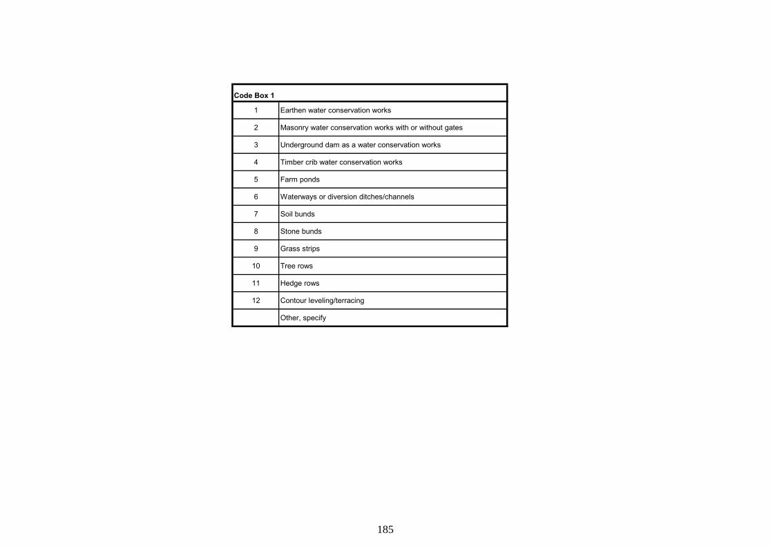
Code Box 1
1 Earthen water conservation works
2 Masonry water conservation works with or without gates
3 Underground dam as a water conservation works
4 Timber crib water conservation works
5 Farm ponds
6 Waterways or diversion ditches/channels
7 Soil bunds
8 Stone bunds
9 Grass strips
10 Tree rows
11 Hedge rows
12 Contour leveling/terracing
Other, specify
185

Section 1: Agriculture
Part 2: Land Management for Household-Managed Plots
1 2 3 5 6 7 8 10 11 12 3Did you leave crop residue on this plot?
If yes, how much? Did you use crop rotation?
Did you practice zero or minimum tillage?
Did you periodically leave this plot fallow?
Did you use precision land leveling/laser land leveling?
Did the plot has soil and water conservation structures?
Did you use cover crops?
Did you use labour on this plot?
No of labourer used Total cost (Rs.) Inkind+Cash
0...No >> Q3 0...No 0...No If permanent labourers did
1...Yes 0...No >> Q5 0...No 0...No 0...No 0...No >> Q10 1...Yes 1...Yes work on all plots write total
If the plot had no crop in entire season, then write -99 and go to Q7
1...Yes Rabi 2014-15
Rabi 2015-16
1...Yes 1...Yes 1...Yes 1...Yes amount in 1st row
Code Percent Code Crop code1Crop
code 2Code Code Code Code 1 2 3 Code Code Permanent Temporary Permanent Temporary
1
1
1
1
1
1
Kharif 2015 Kharif 2016
2
2
2
2
2
2
Ra
bi 2
01
5-1
6K
ha
rif
20
16
SE
AS
ON
4
PL
OT
#
Note: List all those PLOTS here and in all the Parts of Section 1 for which answer to Q3 is code 1, 2, 4 or 6 and answer to Q8 is code 2 or 11 in S1P1
9If yes, which structures?
Code Box 1
If rotating crops, which crops did you rotate on this plot?
186

1 Wheat 31 Rice 61 Mango
2 Gram/Chana Daal 32 Maize 62 Banana
3 Masoor Daal 33 Jawar (Sorghum) 63 Guava
4 Other Pulses(Rabi) 34 Bajra (Millet) 64 Apple/Plum/Peach/ Apricot
5 Rapeseed/Mustard 35 Cotton 65 Kino/Malta/Grapefruit
6 Sunflower 36 Sugarcane 66 Citrus
7 Other Oilseeds 37 Sugar-beets 67 Grapes
8 Potato 38 Moong Daal 68 Pomegranate
9 Onion 39 Mash Daal 69 Dates
10 Tomato 40 Other Kharif pulses 70 Mulberry
11 Peas 41 Groundnuts/Peanuts 71 Persimmon
12 Other Rabi vegetables 42 Sesamum 72 Nuts
13 Spices 43 Soybean 73 Tree for Wood
14 Tobacco 44 Castorseed 74 Firewood
15 Barseem/Lucern 45 Gwaraseed 75 Roses/cut flower
16 Oats 46 Other oil seed (Kharif) 76 Bamboo
17 Other Rabi fodder 47 Chilies 77 Strawberry
50 Melons Other fruits (specify)
51 Water melons
Code Box 2 (Codes for By-products)
6 = Rice husk
1 = Wheat straw 7 = Maize comb
2 = Sugarcane toppings 8 = Maize straw
3 = Sugarcane dry leaves 9 = Millet straw
4 = Cotton sticks Other (specify)
5 = Rice straw
0 = No By-product >> Next crop/plot
Code Box 1 (Crops Grown)
Orchard Code (61-90)Rabi Crops (01-30) Kharif Crops (31-60)
187

Section 1: Agriculture
Part 3: Crop Production in the Past Year (Rabi 2015-16 and Kharif 2016) for Household-Managed Plots
1. 6. 7. 8a. 8b.
Crop name Reason for loss Amount lost after harvest
Reason for post-harvest loss
1 Drought/Water shortage >>Q9a
9a. 9b. 10a. 10b. 10c.
2 Flood
3 Pest/disease
4 Heavy rainfalls If no loss, write 0 >> Q10a
5 Winds
6 Loss during harvesting
7 Frost
8 Fire
Other (specify)
NAME AREA UNIT YEAR MONTH CODE MONTH CODE QUANTITY UNIT QUANTITY CODE QUANTITY CODE NO QUANTITY CODE BOX 2 RS. RS.
1
1
1
1
1
1
1
1
1
1
2
2
2
2
2
2
2
2
2
2
10.
By-products
Name Total value Value of soled out
Loss due to water shortage
How many times you could not irrigate this crop in whole croping season?
9.
6b.1 kilogram2 Mound of 40 Kg3 Mound of 50 Kg4 Mound of 60 Kg
4c. 1= Early 2= Mid 3= Late
-77 = Don't Remember
5.
How much [crop] was harvested during this season?If contract farming, write -44 >> Next cropNote: Report quantity in next questions of Section 1 in the unit used for this question
Time of harvest
If you were provided water according to your needs how much quantity you could extra produce?
1 Insufficient drying of grain2 Poor storage conditions3 Losses during transport4 Defective packaging5 Rain6 TheftOther, specify
6a.Quantity
Instructions for Q5a: i) If flood destroyed the crop completely,then write -44 in Q5a & go to Q6a ii) If an Orchard is immature, then write -99 in Q5a & go to next crop
Area planted 1 Marla2 Kanal3 Bigha / Jareb4 Acre5 Square
2.
5b. 1= Early 2= Mid 3= Late
-77 = Don't Remember
3.
Total loss until harvest (including harvest)
5a. Month (Write 1 for January, 2 for February
and so on)
4.
Planting date
4a. Year
(Write year for orchards &
the crops planted before
2011, and write -44 for
all other crops)
If no loss, write 0 >> Q9a
-77 Don't know
Rab
i 20
15-1
6K
har
if 2
016
SE
AS
ON
Note: Copy PLOT No. from S1P2
4b. Month (Write 1 for January, 2 for February
and so on)
PL
OT
#
CROP CODE
(If the plot had no crop in
entire season, then write
-44 and go to Next Plot)
188

CODE BOX 1: Buyer of Crop CODE BOX 2: Place of Sale
1 Landlord 7 Commission agent in market 1
2 Input dealer 8 Commission agent in village 2
3 Middleman 9 Household/friend 3
4 10 Village shopkeeper 4
5 11 Government 5
6 Wholesaler Other (specify) -77
Farm gate
Market
Other (specify)
Don't know/remember
Retailer in main market
Processor (factory)
Local market
District market
Home, warehouse, or storage place
189

Section 1: AgriculturePart 4: Crop Sales in the Past Year (Rabi 2015-16 and Kharif 2016)
1 2 3 4 5 6 7 8 9 10 11
Quantity kept as feed for livestock
Quantity paid to laborers
Quantity given to the landlord
Total amount sold
Write -99 if no sharecropping
QUANTITY QUANTITY QUANTITY QUANTITY QUANTITY QUANTITY QUANTITY RS./UNIT CODE BOX 1 CODE BOX 2 KM
1
1
1
1
1
1
1
1
1
2
2
2
2
2
2
2
2
2
CR
OP
CO
DE
Ra
bi
20
15
-16
Kh
ari
f 2
01
6S
EA
SO
N
Note: Report quantity in the unit used for question 6 of S1P3
Quantity given away as gifts or in exchange for other goods
Quantity kept by own household (home consumption plus storage)
Quantity kept as seed for next season
Instruction for Q8: For the Orchard or crop for which there is contract farming in S1P3, write total value of sale in Q8 after writing crop code
If not sold out, write -99 >> Q12
What was the price per unit for sold [CROP]?
Who bought most of the crop?
Where was the crop sold?
Distance to location where output was sold
If distance is less than 1 Km, write 0
190

Section 1: AgriculturePart 5: Manure, Compost & Chemical Fertilizers
1. 2. 3. 4. 5. 6. 7. 8.
1 DAP
2 Urea0 No 0 No 0 No 3 2323
1 Yes 1 Donkey load (=1 maund) 1 Yes 1 Donkey load (=1 maund) 4 Other Nitro-Phos blend2 Cart load (=20 maund) 2 Cart load (=20 maund) 1 Yes 5 Potash3 Trolley load (=80 maund) 3 Trolley load (=80 maund) 6 Gypsum
2a.NO. OF LOADS
2b.LOAD UNIT CODE
6a.NO. OF LOADS
6b.LOAD UNIT CODE RS./BAG
SE
AS
ON
Ra
bi
20
15
-16
Kh
ari
f 2
01
6
1
1
1
1
1
1
2
2
2
2
2
2
Report every type of fertilizer used for crop
PL
OT
#
CR
OP
#
Did you use any manure on this ..[PLOT-CROP]..?
How much manure did you use on this ..[PLOT-CROP]..? ..[Fertilizer}.. price per 50kg bag
If sharecropped plot, make sure that tenant reports TOTAL amount used, not just his own share
Did you use any compost on this ..[PLOT-CROP]..?
How much compost did you use on this ..[PLOT-CROP]..?
If sharecropped plot, make sure that tenant reports TOTAL amount used, not just his own share
ENUMERATORS: Plot and Crop #s should be copied from Part 3 of Section 1
CODE CODE CODE CODE NUMBER OF BAGS
► Q3 ► Q5 ► NEXT PLOT-CROP / NEXT SEASON
NOTE: If sharecropped plot, make sure that tenant reports TOTAL amount used not just his own share
Did you use any chemical fertilizer on this ..[PLOT-CROP].. during ..[SEASON]…?
What types of fertilizers did you use on this ..[PLOT-CROP].. during ..[SEASON]…?
Total number of 50kg bags of ..[FERTILIZER TYPE]..
191
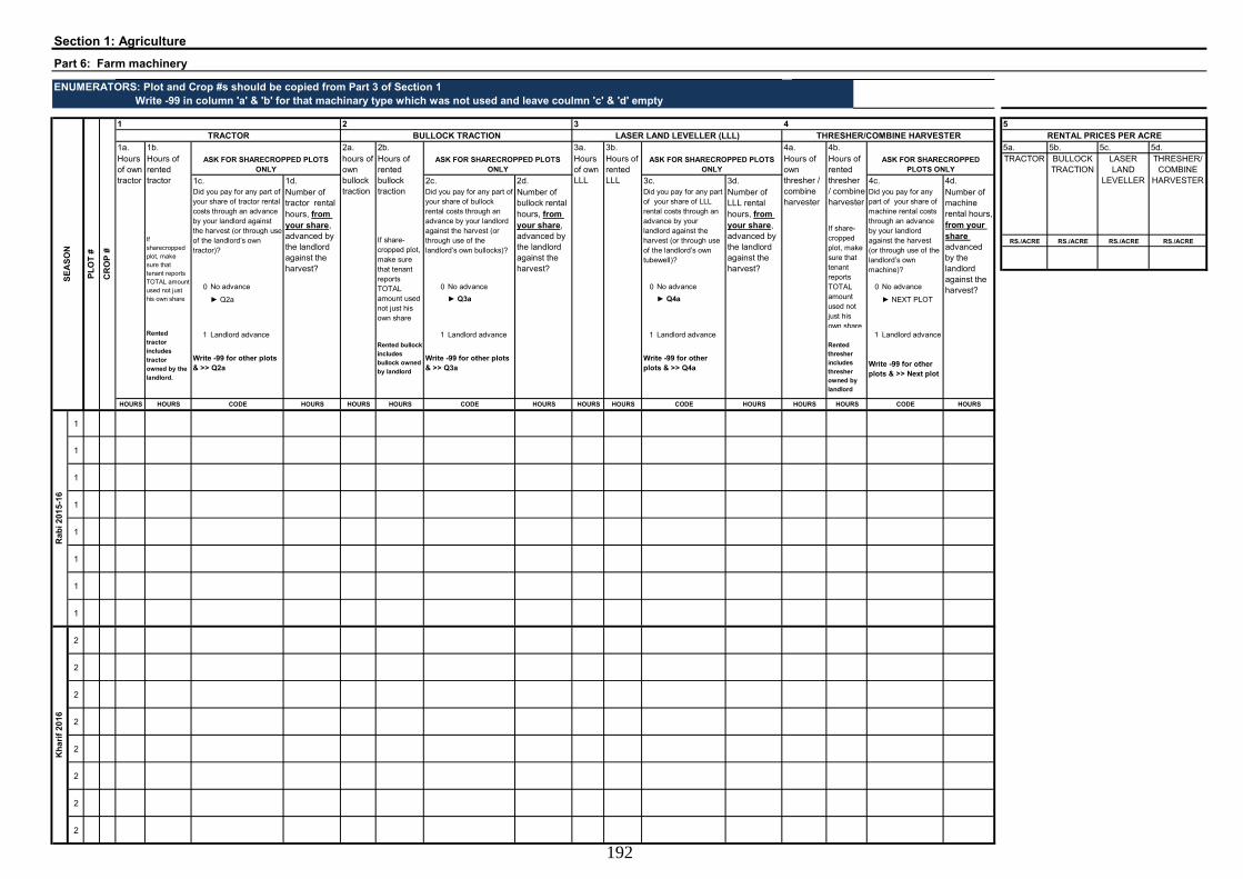
Section 1: Agriculture
Part 6: Farm machinery
1a. 1b. 2a. 2b. 3a. 3b. 4a. 4b. 5a. 5b. 5c. 5d.
1c. 1d. 2c. 2d. 3c. 3d. 4c. 4d.
RS./ACRE RS./ACRE RS./ACRE RS./ACRE
0 No advance 0 No advance 0 No advance 0 No advance
► Q2a ► Q3a ► Q4a ► NEXT PLOT
1 Landlord advance 1 Landlord advance 1 Landlord advance 1 Landlord advance
1
1
1
1
1
1
1
1
2
2
2
2
2
2
2
2
Ra
bi 2
01
5-1
6K
ha
rif
20
16
SE
AS
ON
Number of tractor rental hours, from your share, advanced by the landlord against the harvest?
Did you pay for any part of your share of tractor rental costs through an advance by your landlord against the harvest (or through use of the landlord’s own tractor)?
HOURS CODE
Hours of own thresher / combine harvester
Did you pay for any part of your share of machine rental costs through an advance by your landlord against the harvest (or through use of the landlord’s own machine)?
Number of LLL rental hours, from your share, advanced by the landlord against the harvest?
Number of bullock rental hours, from your share, advanced by the landlord against the harvest?
Did you pay for any part of your share of LLL rental costs through an advance by your landlord against the harvest (or through use of the landlord’s own tubewell)?
HOURS HOURSHOURS
Write -99 for other plots & >> Q2a
Write -99 for other plots & >> Q3a
Write -99 for other plots & >> Q4a Write -99 for other
plots & >> Next plot
Rented tractor includes tractor owned by the landlord.
Rented bullock includes bullock owned by landlord
Rented thresher includes thresher owned by landlord
Number of machine rental hours, from your share advanced by the landlord against the harvest?
If share-cropped plot, make sure that tenant reports TOTAL amount used not just his own share
If sharecropped plot, make sure that tenant reports TOTAL amount used not just his own share
If share-cropped plot, make sure that tenant reports TOTAL amount used not just his own share
TRACTOR BULLOCK TRACTION
LASER LAND
LEVELLER
THRESHER/ COMBINE
HARVESTERDid you pay for any part of your share of bullock rental costs through an advance by your landlord against the harvest (or through use of the landlord’s own bullocks)?
Hours of rented LLL
HOURS HOURS HOURS HOURS CODE HOURSHOURS CODE HOURS HOURS
ENUMERATORS: Plot and Crop #s should be copied from Part 3 of Section 1 Write -99 in column 'a' & 'b' for that machinary type which was not used and leave coulmn 'c' & 'd' empty
CR
OP
#
PL
OT
#
4 5TRACTOR BULLOCK TRACTION LASER LAND LEVELLER (LLL) THRESHER/COMBINE HARVESTER RENTAL PRICES PER ACRE
1 2 3
ASK FOR SHARECROPPED PLOTS ONLY
ASK FOR SHARECROPPED PLOTS ONLY
ASK FOR SHARECROPPED PLOTS ONLY
CODE
Hours of rented thresher / combine harvester
ASK FOR SHARECROPPED PLOTS ONLY
Hours of own tractor
Hours of rented tractor
hours of own bullock traction
Hours of rented bullock traction
Hours of own LLL
192

Code Variety Name Code Variety Name Code Variety Name Code Variety Name Code Variety Name Code Variety Name Code Variety Name Code Variety Name Code Variety Name Code Variety Name
1 Abdul Sattar 26FAISALABAD-08
51 PASBAN 90 76 Uqab-2000 101 493/97 126 CIM-443 151 FH-685 176 MNH-552 201 Basmati Kernal 226 Pusa
2 AARI 2011 27 Faisalabad-2002 52 PAVON 77 Watan-93 102 840/97 127 CIM-446 152 FH-87 177 MNH-554 202 Basmati Super 227 Ranbir
3 ARZ 28FAISALABAD-83
53 PB. 85 78 WL 711 103 AEC/73/3/89 128 CIM-448 153 FH-900 178 MNH-886 203 Basmati-198 228 RH-10
4 AS.2002 29 Fareed-06 54 POTHOWAR 79 YECORA 104 Ali Akbar-703 129 CIM-465 154 FH-901 179 MVH-518 204 Basmati-2000 229 Safidon
5 AUQAB 2000 30 FSD. 85 55 Punjab 2001 80 83 105 Ali Akbar-802 130 CIM-467 155 FH-941 180 NEELAM-121 205 Basmati-217 230 Shahanshah
6 BARANI-70 31 Gandam-711 56 PUNJAB 76 81 3094 106 Ali Akbar-905 131 CIM-473 156 FH-942 181 NIAB-78 206 Basmati-370 231 Shaheen basmati
7 BARANI-83 32 INQILAB 91 57 PUNJAB 81 Other (specify) 107 A-one 132 CIM-482 157 FS-631 182 NIAB-111 207 Basmati-385 232 Suganda
8 Bhakhar-02 33 IQBAL2000 58 PUNJAB 96 108 B32/97 133 CIM-483 158 FVH-137 183 NIBGE-115 208 Basmati-386 233 Taraori
9BHAWALPUR-79
34 Kainat 59 PUNJNAD 88 109 B-496 134 CIM-496 159 FVH-28 184 NS-141 209 Bihar Other (specify)
10 BLUE SILVER 35 KOHINOOR 83 60 RAWAL 87 110 B-622 135 CIM-499 160 FVH-49 185 RH-500 210 Dehradun
11 C217 36 KOHISTAN 97 61 Resham 111 B-803 136 CIM-506 161 FVH-53 186 S-12 211 Fakhre Malakand
12 C228 37 Kohsar-95 62 ROHTAS 90 112 B-820 137 CIM-573 162 FVH-55 187 S-14 212 GNY 50
13 C250 38 LASANI.08 63 SA 42 113 B-821 138 CIM-598 163 FVH-57 188 Sitara-008 213 GNY 53
14 C271 39 LU 26S 64 SA 75 114 B-842 139 CIM-768 164 GM-2085 189 SITARA-009 214 Haryana
15 C273 40 LYALLPUR-73 65 SANDAL 73 115 B-850 140 Desi Ravi 165 IR-1524 190 SLH-317 215 Irri-6
16 C518 41 Mairaj-06 66 SATLUJ 86 116 B-896 141 DNH-49 166 IR-3701 191 SLS-1 216 Irri-9
17 C591 42 MEXIPAK 67 SEHER 06 117 BH-100 142 FDH-170 167 IR-NIBGE-3 192 TARZAN-1 217 JP-5
18 Chakwal - 50 43 MH 97 68 SH.2002 118 BH-118 143 FH-113 168 IR-NIBGE 901 193 TCD-3H 218 Kasturi
19 CHAKWAL-86 44 Millat 2011 69 SHAFAQ 06 119 BH-160 144 FH-114 169 Karishma 194 TSR23-75 219 KS-282
20 Chakwal-97 45 Ms-2011 70 SHAHKAR 95 120 BH-167 145 FH-628 170 MG-6 195 VH-259 220 KS-282
21 CHENAB-2000 46 Nawab 71SHALIMAR 88
121 BH-95 146 FH-629 171 MIAD-852 196 VS-135 221 KSK-133
22 CHENAB-70 47 Nayab 72 Shehzor 122 CIM-109 147 FH-634 172 MNH-93 Other (specify) 222 Mahi
23 CHENAB-79 48 PAK 81 73 Soraj 123 CIM-1100 148 FH-649 173 MNH-465 223 PB2 (Sugandh-2)
24 DIRK 49 PARI 73 74 TD-1 124 CIM-240 149 FH-657 174 MNH-516 224 PB3
25 Durum-97 50 PARWAZ 94 75 Ufaq-02 125 CIM-435 150 FH-682 175 MNH-536 225 Pukhraj
Wheat RiceCotton
193

Section 1: AgriculturePart 7: Other purchased inputs for household managed plots
PESTICIDES/HERBICIDES/FUNGICIDES ELECTRICITY/STORAGE COSTS
3A. 3B. 4A. 4B. 4C. 5A. 5B.
1A. 1B. 2A. 2B. 2C. 2D 2E 2F Total cost of abiana
Type Total Cost
12 1 Grain yield3 2 Grain size4 3 Disease/pest resistance5 4 Drought resistance 0 Not used 6 5 Flood resistance ► Q4A7 6 Low labor needs 1 Insecticide8 7 Low input needs 2 Weedicide9 8 Ease of processing 3 Funjicide 0 No ►Q5A
10 9 Market demand 4 Micro 1 Yes
10 Taste nutrients
11 Color
12 Fodder qualityOther (specify)
KM CODE1 CODE2 CODE Rs.Rs.Rs.CODECODE
Ra
bi
20
15
-16
Kh
ari
f 2
01
6
1
1
1
1
1
2
2
2
2
2
SE
AS
ON
Write -44, if seed is exchanged
SEEDS
Input dealerLandlordResearch institutePunjab Seed CorporationAgri. Extension Department
How long is distance from your house to this supplier ?
Source of purchased seed
Relative (not HH member)Friend/NeighbourIf own seed
not used, then write -44 & go to Q2A
Private seed company
Rs. Rs.
ABIANA/AGRICULTURAL TAX
1. Own Seed
Did you pay any agricultural tax?
Total cost of agricultural taxVariety Quantity Variety Quantity Cost
2. Purchased Seed
In your opinion, what are the two most important traits in seed of this crop?
Total electricity cost
Total storage cost
NOTE : If sharecropped plot, make sure that tenant reports TOTAL COST not just his own share
NOTE : If sharecropped plot, make sure that tenant reports TOTAL COST not just his own share
NOTE : If sharecropped plot, make sure that tenant reports TOTAL COST not just his own share
If not paid, write 0
PL
OT
#
KgsCODE
ENUMERATORS: Plot and Crop #s should be copied from Part 3 of Section 1
KgsCODE
NGO or relief agency
Cooperative societyOther (specify)
CR
OP
#
Rs./Kg
194

Section 2: Agricultural Water UsePart 1: General
Did the household irrigate any plots in last year ((Rabi 2015-16 and Kharif 2016)? 0 No >> Section 3 1 Yes
1. 2. 3. 4. 5. 6. 7. 8. 9. 10. 11. 12. 13. 14.Usual irrigation depth
Distance of plot
from mogha?
0 No >> Q4 0 No
1 Rainfall 1 Rainfall 1 Rainfall 1 Flood 1 Gravity 1 Gravity
2 River 2 River 2 River 2 Furrow 2 Treadle pump 2 Treadle pump
3 Canal 3 Canal 3 Canal 3 Bed and furrow 1 Dug well 3 Rower pump 3 Rower pump
4 Pond 4 Pond 4 Pond 4 Bucket/hose 2 Shallow tubewell 4 Diesel pump 1 Head 4 Diesel pump
5 Lake 5 Lake 5 Lake 5 Sprinkler/Drip 3 Deep tubewell 5 Electric Pump 2 Middle 5 Electric Pump
6 Groundwater 6 Groundwater 6 Groundwater Other (specify) 6 Tractor pump 3 Tail 6 Tractor pump
7 Sewerage water 7 Sewerage water 7 Sewerage water 7 Bucket/hose 7 Bucket/hose
Other (specify) Other (specify) Other (specify) Other (specify)
CODE CODE CODE INCHES INCHES CODE CODE FEET YEAR CODE KM CODE NAME
If the canal is a source of water
Water extraction methodWhere is the plot located?
0 Canal water not used >> Next Crop/Plot
Rab
i 20
15-1
6
Type of irrigation method (applies to both SW and GW)
Tertiary source of water Maximum irrigation depth If groundwater is a source of waterWater extraction method
Kh
arif
201
6
ENUMERATORS: Plot and Crop #s should be copied from Part 3 of Section 1 Note: Ask all of SECTION 2 at the plot level (rather than plot-crop level) and write -44 in CROP #, UNLESS the plot uses drip irrigation in which case we can ask at the plot-crop level
Depth of well
0 GW not used>> Q10
What was the well type? What year was the well drilled?
SE
AS
ON
PL
OT
#
CR
OP
#
Primary source of water Secondary source of water
CODE
Other (specify)
Name of the minor/ distributary that feeds this watercourse
195
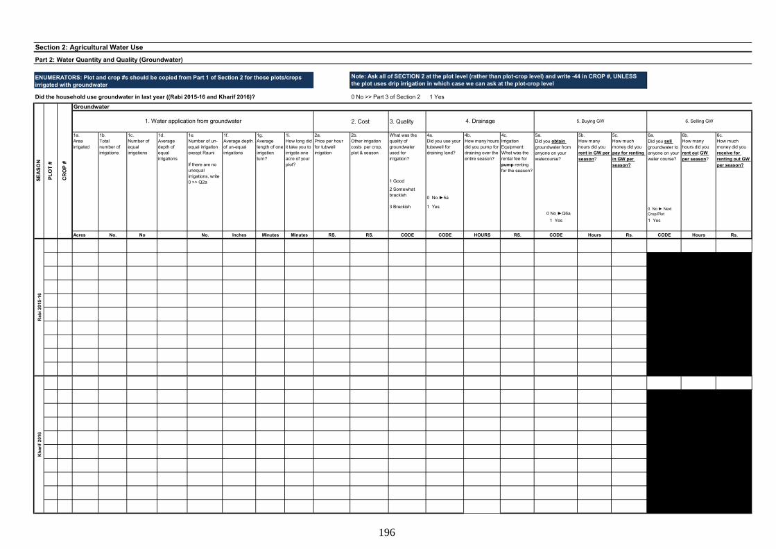
Section 2: Agricultural Water Use
Part 2: Water Quantity and Quality (Groundwater)
Did the household use groundwater in last year ((Rabi 2015-16 and Kharif 2016)? 0 No >> Part 3 of Section 2 1 Yes
Groundwater
2. Cost 3. Quality
1d.Average depth of equal irrigations
1f.Average depth of un-equal irrigations
What was the quality of groundwater used for irrigation?
1 Good
0 No ►5a
3 Brackish 1 Yes
0 No ►Q6a
1 Yes 1 Yes
Acres No. No No. Inches Minutes Minutes RS. RS. CODE CODE HOURS RS. CODE Hours Rs. CODE Hours Rs.
Ra
bi 2
01
5-1
6
6c.How much money did you receive for renting out GW per season?
6b.How many hours did you rent out GW per season?
6a.Did you sell groundwater to anyone on your water course?
Kh
ari
f 2
01
6
0 No ► Next Crop/Plot
5b.How many hours did you rent in GW per season?
5c.How much money did you pay for renting in GW per season?
1g.Average length of one irrigation turn?
1i.How long did it take you to irrigate one acre of your plot?
2a.Price per hour for tubwell irrigation
5a.Did you obtain groundwater from anyone on your watecourse?
PL
OT
#
SE
AS
ON
CR
OP
#
1. Water application from groundwater
4c.Irrigation Equipment: What was the rental fee for pump renting for the season?
2 Somewhat brackish
4a.Did you use your tubewell for draining land?
6. Selling GW
ENUMERATORS: Plot and crop #s should be copied from Part 1 of Section 2 for those plots/crops irrigated with groundwater
Note: Ask all of SECTION 2 at the plot level (rather than plot-crop level) and write -44 in CROP #, UNLESS the plot uses drip irrigation in which case we can ask at the plot-crop level
4b.How many hours did you pump for draining over the entire season?
4. Drainage
2b.Other irrigation costs per crop, plot & season
1a.Area irrigated
1b.Total number of irrigations
1c.Number of equal irrigations
5. Buying GW
1e.Number of un-equal irrigation except Rauni
If there are no unequal irrigations, write 0 >> Q2a
196

Section 2: Agricultural Water Use
Part 3: Water Quantity and Quality (Canal Water)
Did the household use canal water in last year (Rabi 2015-16 and Kharif 2016)? 0 No >> Section 3 1 Yes
Canal Water
3. Timing 5a. Cost5b. other
surface cost5c. Cost 5d. Cost 5e. Cost
6a. Share of irrigation
6b. Share of irrigation
7a. Exchanging Turns
7b. Exchanging Turns
7c. Exchanging Turns
8a. Purchasing turns
8b. Buying turns
8c. Selling turns
8d. Selling turns
1e.
Average depth of irrigations
0 No turns
1 = tail
0 No 0 No ► Q8a 2= head 1=Cash 1=Cash
1 Yes 2 Most turns 1 Yes 3 = head and tail 2=In kind 2=In kind
3 Few turns 4= neighbor
Acres No. No. No. Inches Minutes Minutes CODE Rs. CODE RS. RS. RS. CODE CODE1 CODE # of turns CODE # of turns CODE # of turns CODE
Kh
ari
f 2
01
6
2. Length of irrigations
Ra
bi 2
01
5-1
6
1d.Number of un-equal irrigation except Rauni
If there are no unequal irrigations, write 0 >> Q2a
2a.Average length of one irrigation turn?
SE
AS
ON
#
PL
OT
#
CR
OP
#
1. Water application from surface water
Payment method for any turns sold
If you did not receive your full share, why not?
Did you exchange any turns with someone else on the canal?
How many irrigation turns did you exchange?
Did you exchange turns toward the tail or head or with a nearby neighbor?
How many turns did you sell to someone else along the canal?
What was the abiana paid? (If not available by plot, put total payment in row 1 for each season and mark with '*')
Did you use a pump to extract water from the canal?
0 NO ► Q6a1 Yes
Irrigation Equipment rental fee for pump renting for the season
Electricity cost per season
Diesel/fuel cost per season and crop
2b.How long did it take you to irrigate one acre of your plot?
ENUMERATORS: Plot and crop #s should be copied from Part 1 of Section 2 for those plots/crops irrigated with canal water
Note: Ask all of SECTION 2 at the plot level (rather than plot-crop level) and write -44 in CROP #, UNLESS the plot uses drip irrigation in which case we can ask at the plot-crop level
Payment method for any turns bought
How many turns did you purchase from someone else along the canal?
If not rented, the write-99
If electricity not used, the write-99
If Diesel / fuel not used, the write-99
1a.Area irrigated
1b.Total number of irrigations
1c.Number of equal irrigations
(Warabandi ) Was the timing of your canal water turn as per your needs?
1 All turns ► Q7a
Did you use your full share of water allocation?
197

CODE BOX 1 CODE BOX 2
1. Information on inputs for crop production 1. Found the advice they provided in the past to be unsuitable or unhelpful
2. Information on climate change
3. Information on inputs for livestock production 2. Am not interested in changing production practices
4. Information on new methods of crop production 3. Do not wish to borrow money
5. Information on new methods for livestock production 4. Do not wish to purchase inputs
6. Information on new crops or crop varieties 5. No extension agents available in this muaza or district
7. Information on new livestock or livestock breeds 6. Not enough extension agents available for all farmers in this muaza or district
8. Information on improving water, soil, forests 7. Did not know about services offered by extension agents
9. Information on obtaining & using fertilizer 8. Extension agents only help farmers with more land than my household has
10. Information on obtaining & using agrochemicals 9. Extension agents only help male farmers
11. Information on obtaining & using improved seeds 10. Extension agents only help farmers who are friends or relatives of local officials or politicians
12. Information on obtaining credit/loans 11. Extension agents only help farmers who are friends or relatives of large landowners
13. Information on marketing crops or livestock 12. Extension agents only help educated farmers
Other (specify) Other (specify)
CODE BOX 3 CODE BOX 4
1. Agricultural research institutions 1. Friends
2. NGOs 2. Religious groups
3. Community-based organizations 3. Civil society groups
4. Bank 4. Local progressive farmers
5. Local farmers organization Others specify
6. Cooperatives
Others specify
198

Section 3: Part-1 Access to Extension
1 2 3 4 5 6 7 8 9 10 11 12 13
Did you receive any information on crop or livestock production within the past year from a source other than extension agent?
0…No >> Q31…Yes
If you received other crop or livestock information, how did you receive it?
1…Radio2…Television3…Mobile phone4…Printed materialsOther (specify)
Had you or any member of your household met with an extension agent within the past year?
0…No >> Q121…Yes
If you met with an extension agent, did the agent visit you, or did you visit the agent?
1…Agent visited you2…You visited agent3…Both 1 & 2
What type of extension activities did you participate in mostly during these meetings?(List 3 most important activities)
1…One-on-one advice2…"Training and visit" activity3…Farmer field school4…Demonstration event5…Farmer organization meetingOther, specify
Distence to extension office
If the extension agent visited you or you visited extension agent, how frequently in the last one year were you visited?
1…Every week2…Every 2 weeks3…Every month4…Every 2 months5…Every 3 months6…Every 4 months5…Every 5 months6…Every 6 months7…Every year
During your most recent meeting with an extension agent, to whom did the extension agent give information/ advice?
1…Male head of household2…Female head of household3…Female spouse of household head4…Other male household member5…Other female household member
During the extension agent's most recent visit, from which organization did the extension agent come from?
1…Government agriculture extension department2…Agricultural research institutions3…NGOs4…Community-based organizations5…Business6…Religious groups7...Civil society groups8...Local progressive farmers9...BankOther (specify)
If you were visited by an extension agent during the last year, what information/ advice was provided to you?
(List 3 most important services provided)
Did the information provided by the extension agent meet your needs?
(Answer for each service provided)
0…No1…Yes, very2…Yes, somewhat
What services would you like to receive that you are not currently receiving?
If you did not meet with an extension agent during the last year, why?
(Multiple answers possible)
Write -99 if answer to Question 3 is YES
CODE CODE CODE CODE KM CODE CODE CODE CODE BOX 1 CODE CODE BOX 1 CODE BOX 2
Activity 1: Service 1: Service 1: Service 1: Reason 1:
Activity 2: Service 2: Service 2: Service 2: Reason 2:
Activity 3: Service 3: Service 3: Service 3: Reason 3:
Section 3: Part-2 Social Networks
1- 2- 3- 4- 5- 6- 7- 8- 9- 10- 11- 12- 13-Are you member of a social organization?
0…No >> Q51…Yes
Which organization member are you?
How active this organization in your local area?
1 Very active2 Moderate actve3 Somewhat active4 Not activeOther, specify
How helpful this organization for you?
1 Very 2 Moderate 3 somewhat 4 Not
If you suffered agriculture related or financial problem from whom you get help?
How can they help you?
1 Financially2 Information only3 Both 1 & 24 New technology adoptionOther, specify
Where they live?
1 Same village 2 Other village in same distt. 3 Village in other distt.4 Other province
Please name the five farmers in your network whom you share and get the information related to agricultural and new technology
Are your family relatives share information related to agricultural and new technology?
0…No >> Next Section1…Yes
Where your relative family members live?
1 Same village 2 Other village in same distt. 3 Village in other distt.4 Other province
Do you exchange information related to agricultural and new technology with them?
0 No >> Next Section1 Yes
How can they help you?
1 Financially2 Information only3 Both 1 & 24 New technology adoptionOther, specify
Please name the five farmers in your network whom you share and get the information related to agricultural and new technology
CODE CODE BOX 3 CODE CODE CODE BOX 4 CODE CODE Names CODE CODE CODE CODE Names
199

BOX 1
1 Fever 10 Cholera
2 General weakness/ weight loss 11 Diarrhea
3 Headach 12 Skin problems
4 Joint pain 13 Eye problems
5 Toothach 14 Flue/Cold
6 Heart problem 15 Asthma
7 Hepatitis 16 Heat stress
8 Restlessness 17 Throught/Lungs problem
9 TB Others
200

Section 4: Climate Change
Part 1: Perceptions of Climate Change and Climate Risk
1 2 4 5 6 7 8 10
Which option best describes your attitude towards climate change?
0 Not at all interested1 Not very interested2 Indifferent3 Somewhat interested4 Very interested
Are you concerned about climate change?
0 Not at all concerned >> Q41 Not very concerned >> Q42 Indifferent >> Q43 Somewhat concerned4 Very concerned
Have you noticed any long-term changes in the average temperature over the last 20 years? (If too difficult: Have you noticed a change in the number of hot days over the last 20 years?)
0 No >> Q61 Yes-77 Don't know >> Q6
If you noticed a change in temperature, then what is change?
1 Increased2 Decreased-77 Don't know
Have you noticed any long-term changes in the average rainfall over the last 20 years? (If too difficult: Have you noticed a change in the number of rainfall days over the last 20 years?)
0 No >> Q81 Yes-77 Don't know >> Q8
If you noticed a change in rainfall, then what is change?
1 Increased2 Decreased-77 Don't know
Have you noticed any long-term changes in rainfall variability over the last 20 years?(If too difficult: Have you noticed a change in pattern of rainfall over the last 20 years?)
0 No >> Q101 Yes-77 Don't know >> Q10
Have you noticed any long-term changes in the frequency of extreme weather events over the last 20 years?(If too difficult: Have you noticed a change in number of climate shocks over the past 20 years?)
0 No >> S5P21 Yes-77 Don't know >> S5P2
Reason 1 Reason 2 Reason 3 Change 1 Change 2 Change 3 Change 1 Change 2 Change 3
CODE CODE CODE CODE CODE CODE CODE CODE CODE CODE CODE CODE CODE CODE CODE CODE
12 13 14 15 16 17 18 19 20 21 22
Do you know climate change can cause human and child health issues?
If you noticed human health issues with changing climate, is these?
What are the three major issues? Have you or your family affected by any climate related health issues?
Which major issues you and your family faced? How severe was the impact of climate change on health?
Is changing climate also affecting child health?
Has changing climate affected child healthfrom your family?
How severe affect was?
How you manage health issues, adult as well as child?
What are the affects/issues?
1 Yes 1 Incresed 1 Yes Write three most severe issues/diseases 1 Less severe 1 Yes 1 Yes 1 Less severe 1 Doctor write three most severe
0 No >> S4P2 2 Decreased 0 No >> Q18 2 Medium 0 No 0 No 2 Medium 2 Own treatment issues to child health
-77 Don't know>>Q15 3 Very severe 3 Very severe 3 Hakeem
Issue 1 Issue 2 Issue 3 Issue 1 Issue 2 Issue 3 4 Nothing Issue 1 Issue 2 Issue 3
CODE CODE Box 1 Box 1 Box 1 CODE Box 1 Box 1 Box 1 CODE CODE CODE CODE CODE Box 1 Box 1 Box 1
If you noticed a change in rainfall variability, what changes have you noticed?(List 3 most important changes)
1 Rains have become more erratic2 Rains come earlier3 Rains come later4 Rains are heavier5 Longer periods of drought Other (specify)
9
If yes to Q2, why are you concerned?
(List 3 most important reasons)
1 Reduced agricultural productivity2 Water scarcity3 Decrease in livestock fodder4 More soil erosion5 Health risks6 Affect income sources7 Increase poverty levels8 Food insecurity9 More natural disasters Others (specify)
3
If you noticed a change in the occurrence of extreme weather events, what changes have you noticed?(List 3 most important changes)
1 More frequent floods2 More frequent drought3 More frequent heatwaves4 More frequent storms5 Less frequent floods6 Less frequent drought7 Less frequent heatwaves8 Less frequent storms Other (specify)
11
201
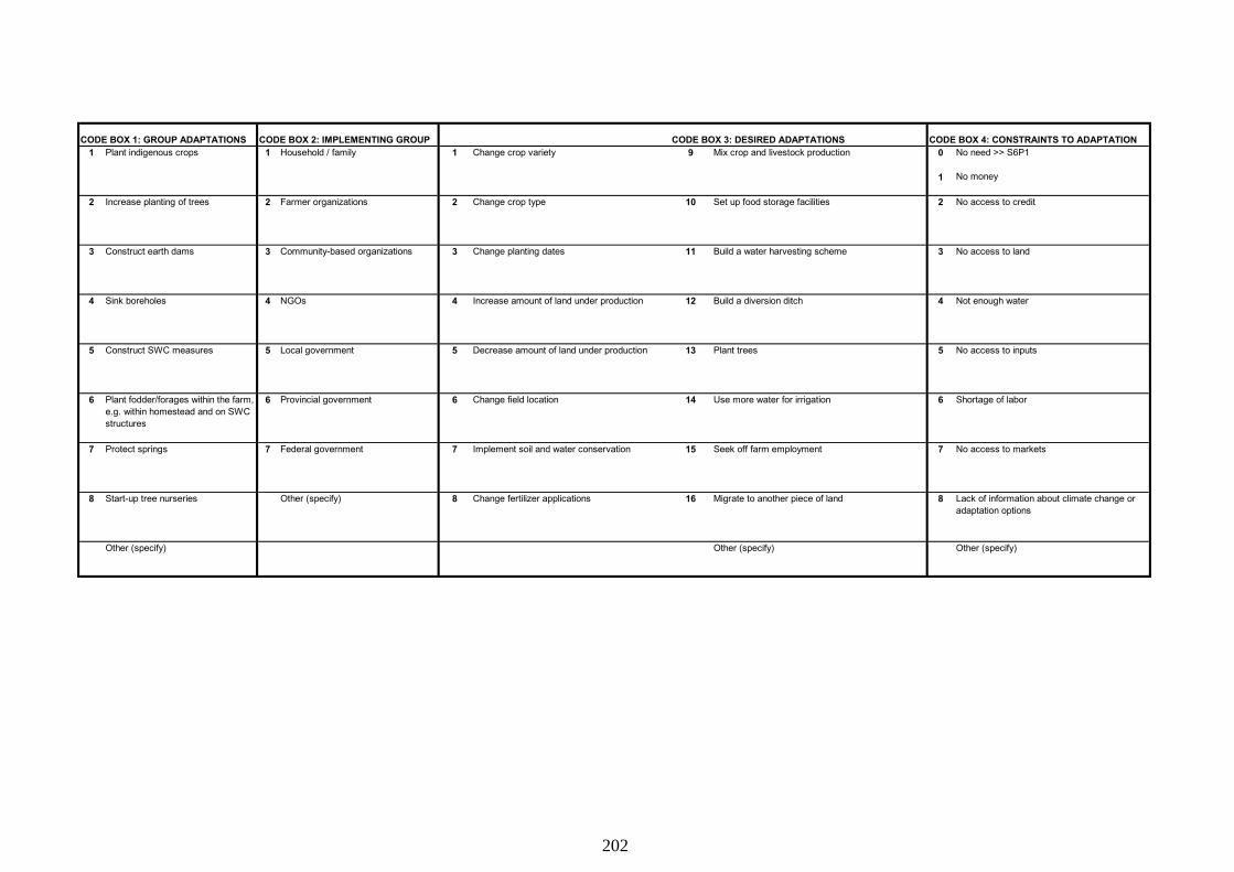
CODE BOX 1: GROUP ADAPTATIONS CODE BOX 2: IMPLEMENTING GROUP CODE BOX 3: DESIRED ADAPTATIONS CODE BOX 4: CONSTRAINTS TO ADAPTATION1 Plant indigenous crops 1 Household / family 1 Change crop variety 9 Mix crop and livestock production 0
1
No need >> S6P1
No money
2 Increase planting of trees 2 Farmer organizations 2 Change crop type 10 Set up food storage facilities 2 No access to credit
3 Construct earth dams 3 Community-based organizations 3 Change planting dates 11 Build a water harvesting scheme 3 No access to land
4 Sink boreholes 4 NGOs 4 Increase amount of land under production 12 Build a diversion ditch 4 Not enough water
5 Construct SWC measures 5 Local government 5 Decrease amount of land under production 13 Plant trees 5 No access to inputs
6 Plant fodder/forages within the farm, e.g. within homestead and on SWC structures
6 Provincial government 6 Change field location 14 Use more water for irrigation 6 Shortage of labor
7 Protect springs 7 Federal government 7 Implement soil and water conservation 15 Seek off farm employment 7 No access to markets
8 Start-up tree nurseries Other (specify) 8 Change fertilizer applications 16 Migrate to another piece of land 8 Lack of information about climate change or adaptation options
Other (specify) Other (specify) Other (specify)
202

Section 4: Climate Change
Part 2: Responses to Climate Change
If the respondent perceives climate change in S5P1, please answer the following questions
1. Have you made any changes in response to climate change in your household or in your community? 0 No >> Q2 1 Yes >> Q3
2. If you have not adapted to climate change, why not? (SEE CODE BOX 4) >> Q7
3a.Change crop variety
0 No1 Yes
3b.Change crop type
0 No1 Yes
3c.Change planting dates
0 No1 Yes
3d.Increase amount of land under production
0 No1 Yes
3e.Decrease amount of land under production
0 No1 Yes
3f.Change field location
0 No1 Yes
3g.Implement soil and water conservation
0 No1 Yes
3h.Change fertilizer applications
0 No1 Yes
3i.Increase fertilizer applications
0 No1 Yes
3j.Decrease fertilizer applications
0 No1 Yes
3k.Build a water harvesting scheme
0 No1 Yes
3l.Build a diversion ditch
0 No1 Yes
3m.Plant trees
0 No1 Yes
3n.Use more water for irrigation
0 No1 Yes
Other (specify)
Other (specify) Other (specify)
4a.Mix crop and livestock production
0 No1 Yes
4b.Change from livestock to crop production
0 No1 Yes
4c.Change from crop to livestock production
0 No1 Yes
4d.Seek off farm employment
0 No1 Yes
4e.Receive training in other livelihood activities
0 No1 Yes
4f.Migrate to another piece of land
0 No1 Yes
4g.Members of the household migrate to an urban area
0 No1 Yes
4h.Set up communal seed banks
0 No1 Yes
4i.Set up food storage facilities
0 No1 Yes
Other (specify) Other (specify) Other (specify)
CODE 4 CODE 4 CODE 4 CODE 4 CODE 4 CODE 4
6b. What are the two main reasons for not adopting desired adaptation 1
6d. What are the two main reasons for not adopting desired adaptation 2
3. What adjustments related to crop production have you made in response to long-term shifts in temperature and rainfall and increased variability?
5c. Group adaptation 2 5e. Group adaptation 3 5g. Group adaptation 4 5i. Group adaptation 5
CODE 2CODE 2
5j. What group or organization implemented group adaptation 5?
5b. What group or organization implemented group adaptation 1?
4. What adjustments to your livelihood or risk mitigation strategies have you made in response to long-term shifts in temperature, rainfall and increased variability?
CODE 1
5h. What group or organization implemented group adaptation 4?
CODE 2CODE 2 CODE 2
5d. What group or organization implemented group adaptation 2?
5f. What group or organization implemented group adaptation 3?
CODE 1 CODE 1
6e. Desired adaptation 3 6f. What are the two main reasons for not adopting desired adaptation 3
6a. Desired adaptation 1
CODE 3 CODE 3 CODE 3
CODE 1
5. Are there any adaptation measures that you have undertaken with other farmers or members of the community in a group? 0 No >> Q7 1 Yes >> Q6a
6. What are your most desired adaptation strategies and constraints to implementing these strategies? (list up to three adaptations and two constraints for each adaptation)
6c. Desired adaptation 2
5a. Group adaptation 1
CODE 1
203

Section 5: Credit
Part 1: Credit rationing
Q.A: Did your household obtain or try to obtain a loan last year ( Rabi 2015-16 and Kharif 2016)? 0 No >> QB 1 Yes >> Q1
Q.B: Why did your household not try to obtain a loan last year (Rabi 2015-16 and Kharif 2016)? >> QB of S5P2
1.- 2.- 3.- 4.- 5.- 6.- 7- 8- 9- 10-How much loan have you obtained from this [LENDER TYPE]?
Did household try toobtain more creditfrom this [LENDERTYPE]?
How much more loan you want to get?
1 Yes
0 No 0 No
1 Yes 1 Yes 0 No
Sr. No. CODE RS. CODE CODE % RS. RS. CODE RS
1
2
3
4
5
6
7
8
9
CODES FOR QUESTION 3: MAIN PURPOSE OF THE LOAN1 Agricultural Production 5 Purchase of tubewell 9 Purchase/Improvement of family dwelling 13 For wedding
2 Purchase of agricultural land 6 Purchase of other farm equipment 10 To pay off old loans Other, specify
3 Purchase of tractor 7 Medical expenses 11 For startup of a non-farm enterprise(s)
4 Purchase of thresher 8 Other Consumption 12 For new investment in a non-farm enterprise(s)
Aarthi/Beopari/Trader
Shopkeeper
RS.
Total amount that stillneeds to be repaid,including all interest andfees.
ACCESS TO CREDIT FOR ALL HOUSEHOLDS
0 No need for loan1 Inadequate collateral2 Had outstanding loan3 Past history of default4 Bad credit history5 Interest rates too high6 Lenders not located nearby7 Procedures too cumbersome8 Need to pay bribes
LENDER TYPE Last 12 months
Was your household successful in obtaining the loan from this [LENDER TYPE]?
What was the main purpose of this loan?
Was any interest charged on this cash loan?
Landlord
Other, specify ___________
DESCRIPTION
Commercial Banks
Zarri Taraqiati Bank
NGO/ Micro-Finance Institution(Specify________________ )
Mill (such as sugar mill, cottonginning factory etc.)
Annual Interest rate (%) or Annual Profit / Munaafa (%)
Additional fees and other costs of getting this loan
How much of what you owe on this loan has been repaid already?
Money lender
Relatives and Friends
204
Section 5: CreditPart 2: Goods and inputs purchased on credit in last year (Rabi 2015-16 and Kharif 2016) This part includes all inputs and/or household consumption goods purchased on cedit in last year (Rabi 2015-16 and Kharif 2016)
A. Did you purchase any input and/or home consumption good on credit in last year (Rabi 2015-16 and Kharif 2016)? 0 No >> S6P1
1 yes
1 2 3 4 5 6 7 8 9 10 11
Items 1 After few days 1 Cash >> Q11
2 after receiving salary 2 Gave harvest output
3 After one month
1 Yes 0 =No>> 6 4 After harvest 0 No
1=Yes 5 Not paid till now >> Next item 1 Yes >> 11
Sr. No. CODE % Rs. CODE Rs. / UNIT Rs.
1Fertilizer
2Seed
3Pesticide
4Diesel
5Other inputs
6
Household consumption goods
What was prevailing market price of [CROP]
How much cash amount did you pay
If Answer to Q7 is only code 2, then don't ask this question
Value of quantity sold
If Answer to Q7 is only code 4, then answer this question and go to Next Item
Did you receive prevailing market prices for [CROP]
From whom did you purchase [ITEM]?
What was the value of [ITEM] purchased on credit?
Did the lender charge you any markup/ commission on the input price or prices (i.e. credit price higher than cash price)?
What was the % markup (average if lender gave several inputs)?
When did you pay for the items?
Other (specify)
1 Landlord
2 Input Dealer
3 Shopkeeper3 Provided labor >> Next item
4 Other in-kind5 Both 1 & 26 Both 1 & 4
CODE CODE
Did you purchase [ITEM] on credit in last year (Kharif 2011 and Rabi 2011-12)?
In what form did you pay?
0 No >> Next item
4 factory
CODE CODE Rs.
205

Section 6: Assets
Part 1: Farm Assets
1 2 3 4 5FARM ASSETS Total value if sold
today?
1 HP2 KwH
3 Litre per second
Year Rs.
01 Large tractor (>=12 HP)
02 Small tractor (<12 HP)
03 Diesel Tubewell
04
05
06
07 Mechanical water pump
08 Machine pulled plow or harrow
09 Animal pulled plow or harrow
10 Combine Harvester
11 Thresher
12 Rice Planter
13 Manual Corn Sheller
14 Mechanical Corn Sheller
15 Chakki
16 Fodder Chopper
17 Motorized insecticide pump
18 Hand insecticide pump
19 Tractor Trolley
20 Animal-driven Cart
21 Generator/ Diesel Engine
Other (specify_____________)
Electric Tubewell
Hand pump (treadle or rower pump)
Sprinkler/drip irrigation
Sr.
No
.Year purchased of the oldest
unit still in operationHow much did you spend on
repairing [FARM ASSET] over past 1 year?
(If jointly owned, report value of share only)
DESCRIPTION NUMBER Rs. Capacity Unit
How many ..[FARM ASSETS].. does your household own?
NOTE: On jointly owned asset, report your share only.
If not owned, write 0 >> Next asset
Engine power or Pump capacity
206

Section 6: Assets
Part 2: Household assets
1. 2. 3. 4.
Total Current value
No…0 >> Next asset
Yes..1
Code (No.) (Rs.)
1 Cooking range/stove
2 Armoire/Cabinet
3 Table / chair
4 Electric fan
5 Electric iron
6 Radio
7 Audio cassette/CD/DVD player
8 Wall clock /watch
9 Television (B/W)
10 Television (Color)
11 Camera/ Video Camera
12 Computer
13 Jewelry (gold/silver) in tolas
14 Sewing machine
15 Bicycle
16 Rickshaw
17 Van (tricycle van)
18 Tonga
19 Push cart
20 Scooter
21 Motorcycle
22 Car
23 Mobile phone set
24 Land phone set
25 Saw
26 Hammer
27 Masons equipment
28 Potters Chaka
29 Blacksmiths Hapor
30 Spade
31 Axe
32 Shovel
33 Guns
34 Refrigerator
35 Water Geyser
36 Freezer
37 Microwave oven
38 Heater
39 Washing machine
40 Air conditioner / cooler
41 Livestock animal
Other (specify: _________________)
Other (specify: _________________)
Description of assetAsset code
Does your household own the item?
Quantity
if asset sold today how much will you receive?
207

Section 6: Assets
Part 3: Savings
Ask for all household members who are 15 years or older. 1. Does any household member (male or female) currently have any savings? 0 No, 1 Yes
2. Has any member of the household (male or female) had any savings in the past 1 year (May 2015-April 2016)? 0 No, 1 YesIf no to both Q1 and Q2, then go to Section 4.
If the individual has more than one “account”, put in separate rows.
3. 4. 5. 6. 7.
PID 1
1
2
3
4
5
6
7
8
9
10
Other, specify ___________________..15
Rs.
Total amount of saving currently in hand
Ask how many accounts each individual (male or female) currently has and list them all. Each “account” should have a separate row.
LIN
E N
UM
BE
R
Saver Where do you save?How do you use / plan to
use the savings? Total amount currently saved
in this place
CODE BOX 1 CODE BOX 2 Rs.
Code Box 1: Where Code Box 2: Use / Intended Use
At home …………..........………………….1 To buy household goods ………………..1
NGO .……………………………….………2 To buy productive assets ………………2
Bank………………………..……………….3 To start / help business …………………3
Shop ………………………………………..4 To buy land / house ……………………..4
Post office / government institution ……..5 For education / training ………………….5
Employer’s provident fund ……………….6 For marriage / dowry …………………...6
Insurance company ………………………7 To build / repair house ………………….7
Relative / friend / neighbor ……………….8 To get loan ……………………………….8
For the future of children ……………...12
Medical emergency …………………….13
Other emergency/natural disaster……..14
Committee/bisi …..…………………….…..9 To lend to others ………………………..9
Other (specify) ______________…...…10 To prepare for difficult times/danger ...10
To send someone abroad for a job …..11
208

Section 7: Other Income
Please tell me the amount (cash and cash equivalency of in-kinds) received during the last year (Rabi 2015-16 and Kharif 2016) from each of the sources
4
Sr. No. NUMBER
1
2
3
4
5
6
7
8
9
10 Net Income from animal products (e.g. milk, butter etc)
11 Net Income from animal soled out
Note: gifts do not include remittances
1 2 3 5Source Did your household receive any amount (cash and cash
equivalency of in-kinds) during the last year (Rabi 2015-16 and Kharif 2016) from [source]?
What was the frequency of receipts? Total Amount
0 No >> Next source 1 Monthly
1 Yes 2 Yearly >>Q5
For how many months, did your household receive any amount during the last year (Rabi 2015-16 and Kharif 2016) from [source]?
CODE CODE
Land rent
Rs
Building rent
Rent from equipment/tools/vehicle
Gifts/ assistance from family or friend
Other (specify): ________________
Rent from animals leased out
Pension
Remittances from a household member who migrated
Net income from land shared out
Net income from animals shared out
209

Section 8: Consumption and ExpendituresPart 1: Frequent Expenditures
Q1 Q2 Q3 Q4Item name In the last 30 days did
your household spend money on [item]?
0 No >> Q41 Yes
CODE Rupees Rupees
1 Fuel (firewood, charcoal, kerosene, gas)
2Expenses on travel (using own or available transport, within or outside village)
3Communication (cell phone, calling cards, phone, postage, internet, faxes)
4 Education (fee, uniform, books, stationary)
5Expenses on utilities and maintenance (electricity, water, maintenance of house, furniture, vehicle)
6 Wages to permanent agricultural labour
7 Wages to permanent non-agricultural labour
8 House Rent (imputed rent if own house)
9 Labour costs of livestock
Other, (e.g., Pan, Cigarette, tobacco etc.)
Part 2: Less Frequent ExpendituresQ1 Q2 Q3Item ID Item name In the last 12 months,
did your household spend money on [item]?
What was your household's total expenditure on [item] over the last 12 months?
0 No >> next item1 Yes
CODE Rupees
1 Clothes and shoes
2 Social events (wedding, funeral, birthdays, etc)
3Housing improvement (latrine, new roof, new room, kitchen, etc)
4Human Health expenses (medication, consultation, hospitalization)
5Cultural/religious activities (e.g. Mela, Milad, quran khwani, etc.)
6 Religious activities like slaughtering on Eid etc.
7 Cost on land shared out
8 Cost on animals shared out
Others____________________
Amount spent on [item] in the last 30 days?
Average monthly expenditure for the last 12 months
Item ID
210

Section 8: Consumption and ExpendituresPart 3a: Food Consumption
1- 2- 3- 4- 5- 6- 7-Item ID Food item name In the last 7 days did your
household spend money on [item]?
How many times [item] used as food in the last 7 days?
How much (average) quantity used in one time?
Price per unit of [item]?
Have you faced the constraint/shortage or any barrier for the purchase of [item]?
How many times in last 30 days?
How many times in last 12 months?
0 No >> Next item1 Yes
0 No >> Next item1 Yes
CODE NO KG RUPEES/KG CODE NO NO
1 Wheat flour
2 Rice
3 Vegetables
4 Pulses (Beans, Peas, Lentils)
5 Meat
6 Fruits
7 Vegetable salad
8 Dessert/Sweet dish
9 Spices
10 Cooking oil/Ghee
11 Milk products
12 Fish
Miscellaneous (Suger, salt, tea… etc.)
211

Section 8: Consumption and Expenditures
Part 3b: Household Food Insecurity Access Scale (HFIAS)
These questions are based on the past four weeks
Q ID QuestionsHow many times in the past four weeks?
1 Did you worry that your household would not have enough food?
2Were you or any household member not able to eat the kinds of foods you preferred because of a lack of resources?
3 Did you or any household member have to eat a limited variety of foods due to a lack of resources?
4Did you or any household member have to eat some foods that you really did not want to eat because of a lack of resources to obtain other types of food?
5Did you or any household member have to eat a smaller meal than you felt you needed because there was not enough food?
6 Did you or any household member have to eat fewer meals in a day because there was not enough food?
7 Was there ever no food to eat of any kind in your household because of lack of resources to get food?
8 Did you or any household member go to sleep at night hungry because there was not enough food?
9Did you or any household member go a whole day and night without eating anything because there was not enough food?
212
![2' · 2013. 7. 5. · '2' ,3 7lsr 7\sh 3ljqrqh&rurqd 3lqlrq&urzq &rssld9horflwj gl urwd]lrqh 5dssruwr gl ulgx]lrqh 7rutxh 5hgxfwlrq udwlr 1p 5rwdwlqj vshhg 530 3xohjjld dyyrojlfdyr9horflwj](https://img.pdfslide.net/doc/110x75/60d76def14068a65a4162d9b/2-2013-7-5-2-3-7lsr-7sh-3ljqrqhrurqd-3lqlrqurzq-rssld9horflwj.jpg)


![H I L B F B A : P B 3 : I J H ; E ? F : M I J : < 4 : 5 ...poincare.matf.bg.ac.rs/~matf/disertacije/Nglis... · 'lvvhuwdwlrq wlwoh 7kh rswlpl]dwlrq ri wkh ehqhilw frvwv wudghrii gxulqj](https://img.pdfslide.net/doc/110x75/5beda2da09d3f2ed1c8cae20/h-i-l-b-f-b-a-p-b-3-i-j-h-e-f-m-i-j-4-5-matfdisertacijenglis.jpg)


![ENGINEERING - NP 2017 - new style A4 - Diamond Tools ... · 5hgxfwlrq À rru À rru wlph &rqvlvwhqf\ ri eruh vl]h &rqvlvwhqf\ ri ¿ qlvk &ruuhfwlrq ri dq\ eruh plvdoljqphqw 6lqjoh](https://img.pdfslide.net/doc/110x75/5b2c3b807f8b9aa6198bee13/engineering-np-2017-new-style-a4-diamond-tools-5hgxfwlrq-a-rru-a.jpg)

![Lilian Maluf Martins - Dissertação - Ed. Corrigida · /,/,$1 0$/8) 0$57,16 (ohfwulflw\ ghilflw frvw hvwlpdwlrq lq %ud]lo e\ dsso\lqj lqsxw rxwsxw dqdo\vlv 'lvvhuwdwlrq 3uhvhqwhg](https://img.pdfslide.net/doc/110x75/5c056f3109d3f2da2e8b46b6/lilian-maluf-martins-dissertaaao-ed-1-08-05716-ohfwulflw.jpg)


![(LQIOXVV ’LDEHWHV DVVR]LLHUWHU 0XWDWLRQHQ LP ... · (lqioxvv ’ldehwhv dvvr]llhuwhu 0xwdwlrqhq lp 7udqvnulswlrqvidnwru +1) a,qdxjxudo ’lvvhuwdwlrq]xu (uodqjxqj ghv ’rnwrujudghv](https://img.pdfslide.net/doc/110x75/5d6179b988c993f1688b64a4/lqioxvv-ldehwhv-dvvrllhuwhu-0xwdwlrqhq-lp-lqioxvv-ldehwhv-dvvrllhuwhu.jpg)


![Einfluss der Entstehung und der Therapie von Epilepsien auf die … · 2016-08-24 · ,qdxjxudo 'lvvhuwdwlrq ]xu (uodqjxqj ghu 'rnwruz ugh ghu 7lhulu]wolfkhq )dnxowlw ghu /xgzlj 0d[lploldqv](https://img.pdfslide.net/doc/110x75/5e5d39961a67a20c4b4b8353/einfluss-der-entstehung-und-der-therapie-von-epilepsien-auf-die-2016-08-24-qdxjxudo.jpg)