Embed Size (px)
Citation preview
6
Output, Price, and Profit:The Importance of Marginal Analysis
● Price and Quantity: One Decision, Not Two
● Total Profit: Keep your Eye on the Goal
● Marginal Analysis and Maximization of Total Profit
● Generalization: The Logic of Marginal Analysis and Maximization
● Price and Quantity: One Decision, Not Two
● Total Profit: Keep your Eye on the Goal
● Marginal Analysis and Maximization of Total Profit
● Generalization: The Logic of Marginal Analysis and Maximization
OutlineOutline
Copyright © 2006 South-Western/Thomson Learning. All rights reserved.
Copyright© 2006 Southwestern/Thomson Learning All rights reserved.
Puzzle: Making Profit by Selling Below CostPuzzle: Making Profit by Selling Below Cost
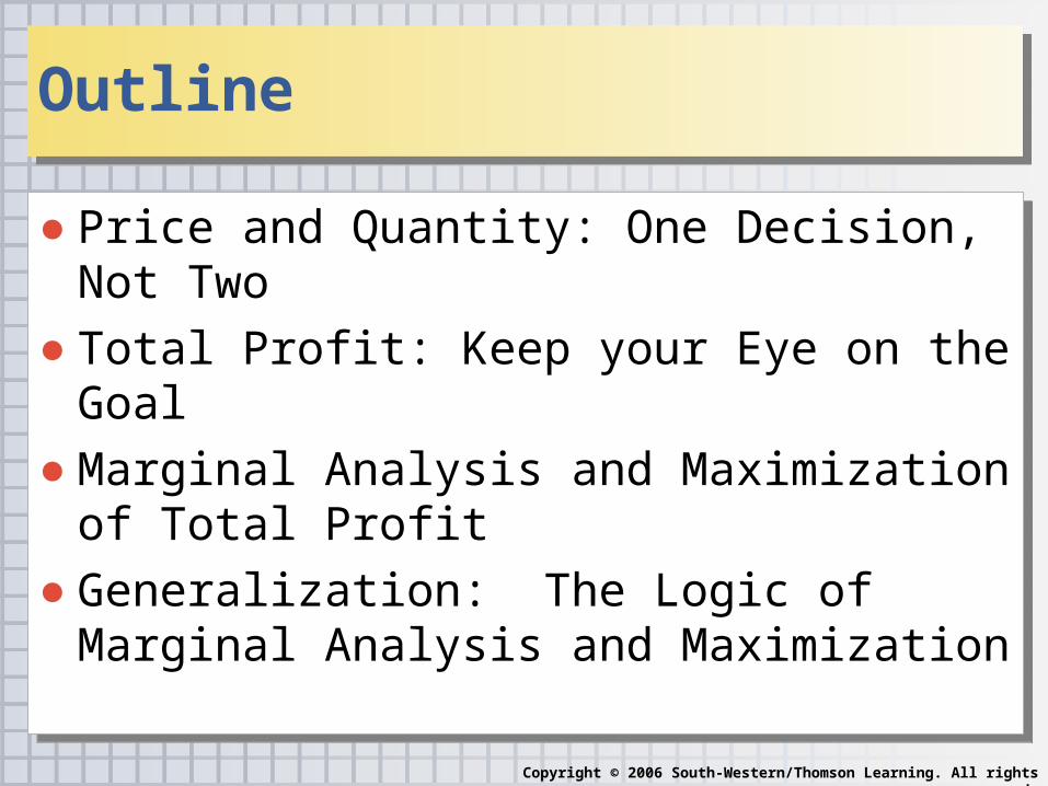
● Legal battle between Co. A and B who make calculators.● B accused A of selling 10M for $12 each, which A knew
was below cost.♦ B claimed A was trying to drive B out of business.
● When A’s cost records were shown in court, looked like B was right.♦ Direct costs of materials, L, and ads = $10.30/unit
♦ Indirect costs of admin. and R& D = $4.25 /unit
♦ So P of $12 did not cover $14.55 cost/unit.
Copyright© 2006 Southwestern/Thomson Learning All rights reserved.
Puzzle: Making Profit by Selling Below CostPuzzle: Making Profit by Selling Below Cost
● Economists defending A showed that its calculator sales were profitable, so it wasn’t just trying to destroy B.
● After discussing profit-max output decisions, you’ll see why A was profitable.
● Economists defending A showed that its calculator sales were profitable, so it wasn’t just trying to destroy B.
● After discussing profit-max output decisions, you’ll see why A was profitable.
Copyright© 2006 Southwestern/Thomson Learning All rights reserved.
Price and Quantity: One Decision, Not TwoPrice and Quantity: One Decision, Not Two
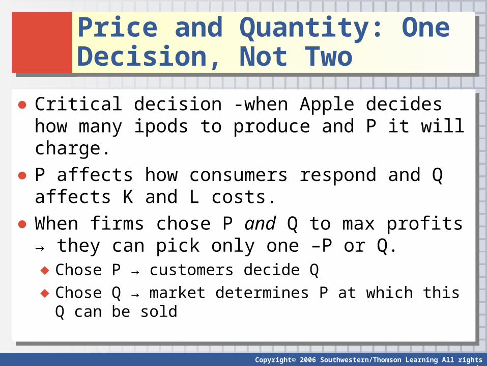
● Critical decision -when Apple decides how many ipods to produce and P it will charge.
● P affects how consumers respond and Q affects K and L costs.
● When firms chose P and Q to max profits → they can pick only one –P or Q.♦ Chose P → customers decide Q
♦ Chose Q → market determines P at which this Q can be sold
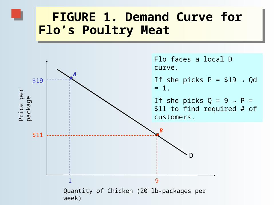
FIGURE 1. Demand Curve for Flo’s Poultry Meat
FIGURE 1. Demand Curve for Flo’s Poultry Meat
D
Quantity of Chicken (20 lb-packages per week)
Pric
e pe
r pa
ckag
e A
1
$19
B
9
$11
Flo faces a local D curve.
If she picks P = $19 → Qd = 1.
If she picks Q = 9 → P = $11 to find required # of customers.
Copyright© 2006 Southwestern/Thomson Learning All rights reserved.
Price and Quantity: One Decision, Not TwoPrice and Quantity: One Decision, Not Two
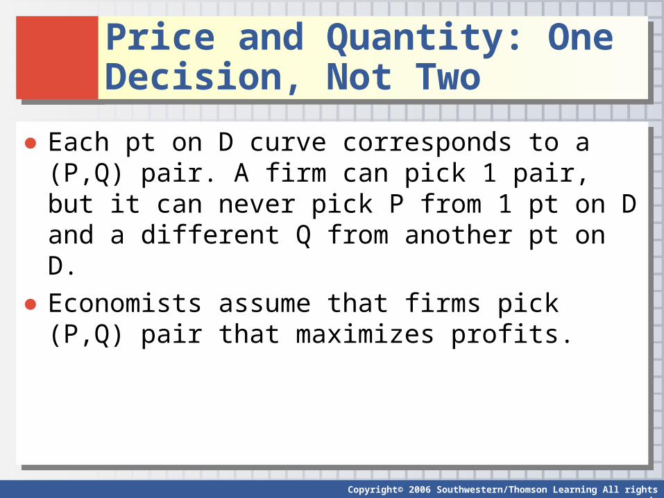
● Each pt on D curve corresponds to a (P,Q) pair. A firm can pick 1 pair, but it can never pick P from 1 pt on D and a different Q from another pt on D.
● Economists assume that firms pick (P,Q) pair that maximizes profits.
● Each pt on D curve corresponds to a (P,Q) pair. A firm can pick 1 pair, but it can never pick P from 1 pt on D and a different Q from another pt on D.
● Economists assume that firms pick (P,Q) pair that maximizes profits.
Copyright© 2006 Southwestern/Thomson Learning All rights reserved.
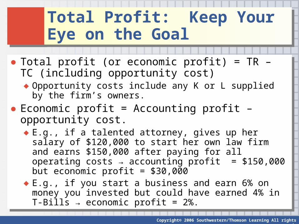
Total Profit: Keep Your Eye on the GoalTotal Profit: Keep Your Eye on the Goal
● Total profit (or economic profit) = TR – TC (including opportunity cost)♦ Opportunity costs include any K or L supplied by the firm’s
owners.
● Economic profit = Accounting profit – opportunity cost.♦ E.g., if a talented attorney, gives up her salary of $120,000 to
start her own law firm and earns $150,000 after paying for all operating costs → accounting profit = $150,000 but economic profit = $30,000
♦ E.g., if you start a business and earn 6% on money you invested but could have earned 4% in T-Bills → economic profit = 2%.
Copyright© 2006 Southwestern/Thomson Learning All rights reserved.
Total Profit: Keep Your Eye on the GoalTotal Profit: Keep Your Eye on the Goal
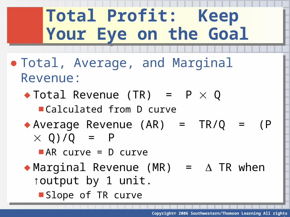
● Total, Average, and Marginal Revenue:♦ Total Revenue (TR) = P Q
■ Calculated from D curve
♦ Average Revenue (AR) = TR/Q = (P Q)/Q = P■ AR curve = D curve
♦ Marginal Revenue (MR) = TR when ↑output by 1 unit.
■ Slope of TR curve
● Total, Average, and Marginal Revenue:♦ Total Revenue (TR) = P Q
■ Calculated from D curve
♦ Average Revenue (AR) = TR/Q = (P Q)/Q = P■ AR curve = D curve
♦ Marginal Revenue (MR) = TR when ↑output by 1 unit.
■ Slope of TR curve
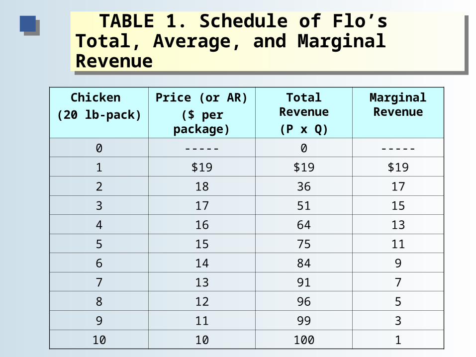
TABLE 1. Schedule of Flo’s Total, Average, and Marginal Revenue
TABLE 1. Schedule of Flo’s Total, Average, and Marginal Revenue
Chicken
(20 lb-pack)
Price (or AR)
($ per package)
Total Revenue
(P x Q)
Marginal Revenue
0 ----- 0 -----
1 $19 $19 $19
2 18 36 17
3 17 51 15
4 16 64 13
5 15 75 11
6 14 84 9
7 13 91 7
8 12 96 5
9 11 99 3
10 10 100 1
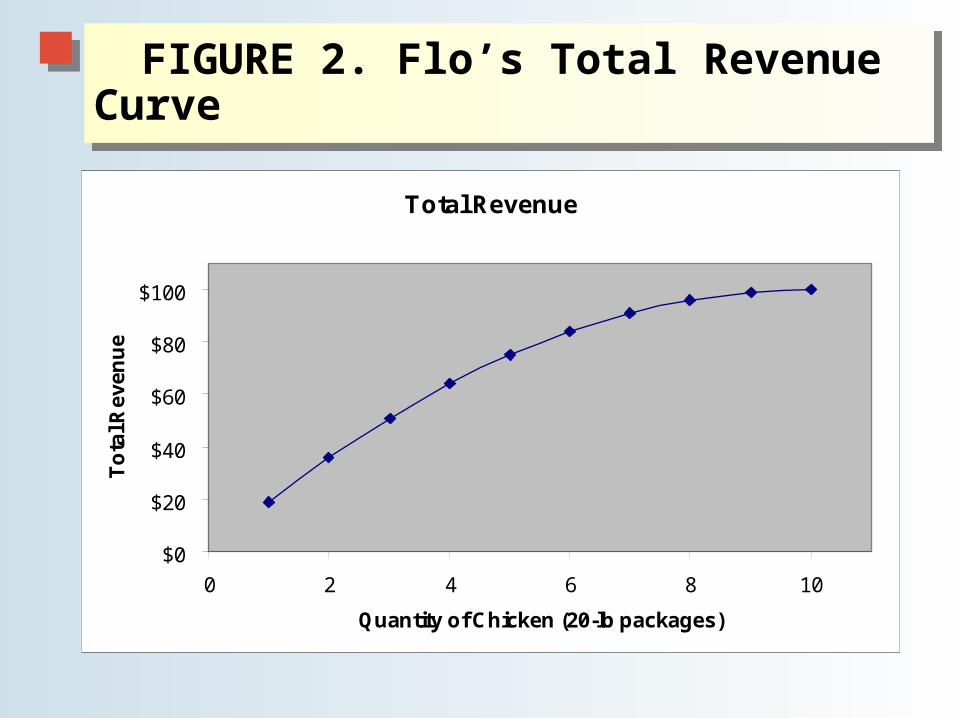
FIGURE 2. Flo’s Total Revenue CurveFIGURE 2. Flo’s Total Revenue Curve
Total Revenue
$0
$20
$40
$60
$80
$100
0 2 4 6 8 10
Quantity of Chicken (20-lb packages)
To
tal R
eve
nu
e
Copyright© 2006 Southwestern/Thomson Learning All rights reserved.
Total Profit: Keep Your Eye on the GoalTotal Profit: Keep Your Eye on the Goal
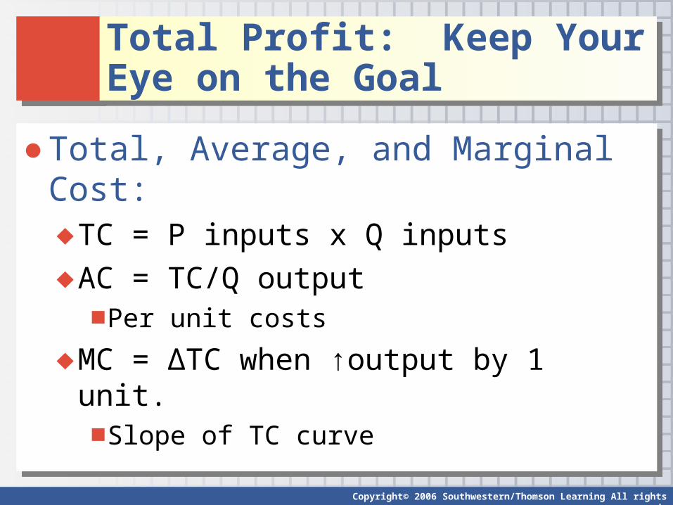
● Total, Average, and Marginal Cost:♦ TC = P inputs x Q inputs
♦ AC = TC/Q output■Per unit costs
♦ MC = ∆TC when ↑output by 1 unit.■Slope of TC curve
● Total, Average, and Marginal Cost:♦ TC = P inputs x Q inputs
♦ AC = TC/Q output■Per unit costs
♦ MC = ∆TC when ↑output by 1 unit.■Slope of TC curve
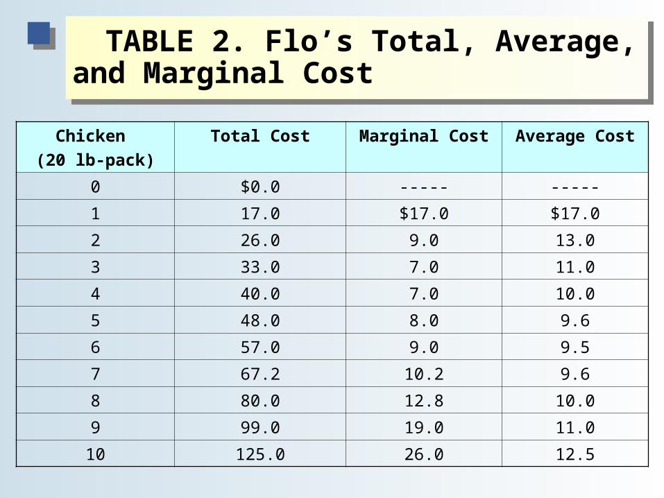
TABLE 2. Flo’s Total, Average, and Marginal Cost
TABLE 2. Flo’s Total, Average, and Marginal Cost
Chicken
(20 lb-pack)
Total Cost Marginal Cost Average Cost
0 $0.0 ----- -----
1 17.0 $17.0 $17.0
2 26.0 9.0 13.0
3 33.0 7.0 11.0
4 40.0 7.0 10.0
5 48.0 8.0 9.6
6 57.0 9.0 9.5
7 67.2 10.2 9.6
8 80.0 12.8 10.0
9 99.0 19.0 11.0
10 125.0 26.0 12.5
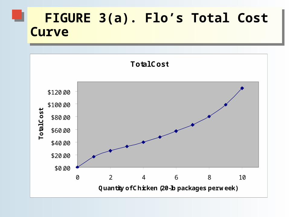
FIGURE 3(a). Flo’s Total Cost CurveFIGURE 3(a). Flo’s Total Cost Curve
Total Cost
$0.00
$20.00
$40.00
$60.00
$80.00
$100.00
$120.00
0 2 4 6 8 10
Quantity of Chicken (20-lb packages per week)
To
tal C
os
t
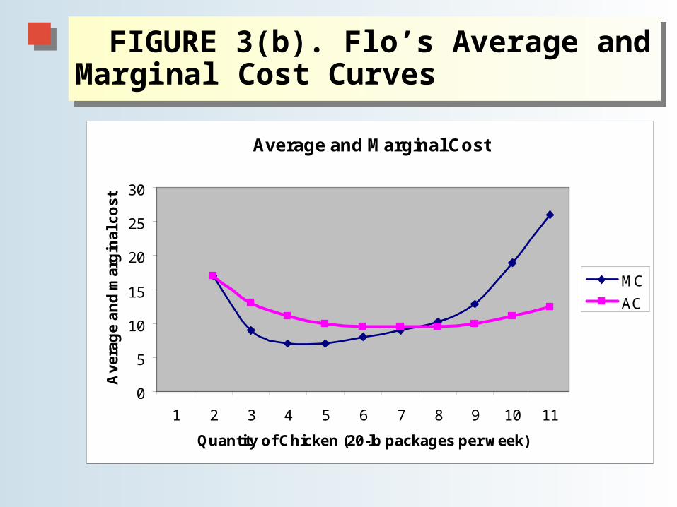
FIGURE 3(b). Flo’s Average and Marginal Cost Curves
FIGURE 3(b). Flo’s Average and Marginal Cost Curves
Average and Marginal Cost
0
5
10
15
20
25
30
1 2 3 4 5 6 7 8 9 10 11
Quantity of Chicken (20-lb packages per week)
Av
era
ge
an
d m
arg
ina
l co
st
MC
AC
Copyright© 2006 Southwestern/Thomson Learning All rights reserved.
Total Profit: Keep Your Eye on the GoalTotal Profit: Keep Your Eye on the Goal
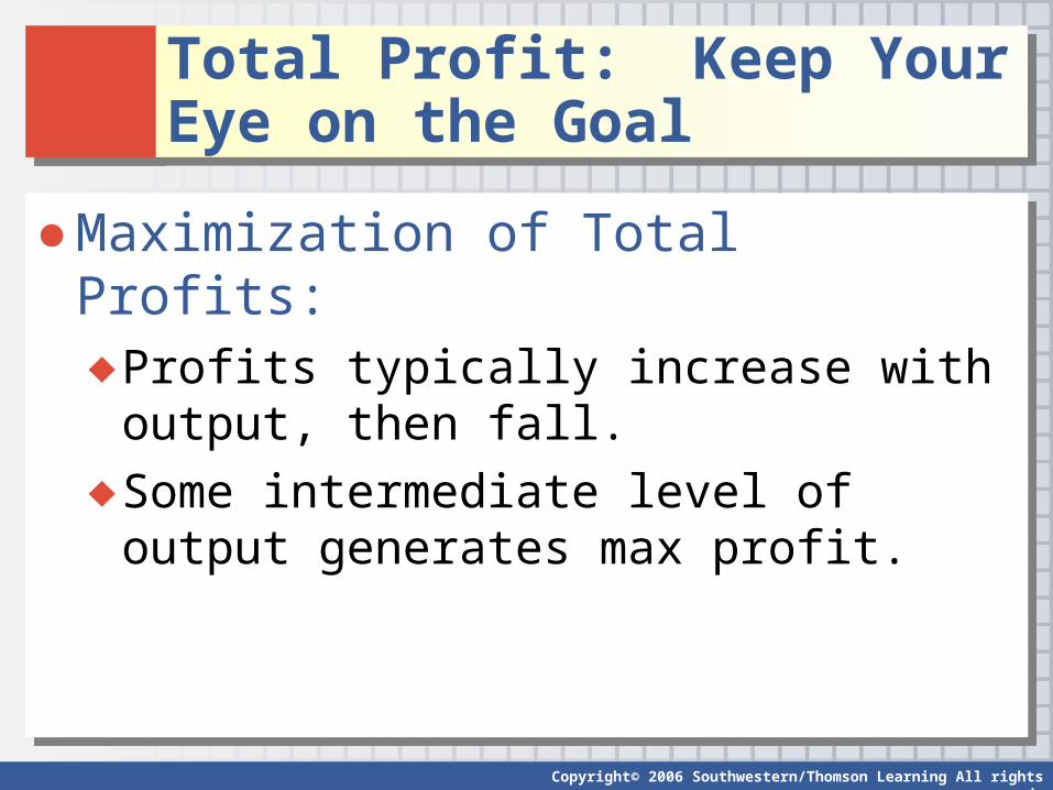
● Maximization of Total Profits:♦ Profits typically increase with output, then fall.
♦ Some intermediate level of output generates max profit.
● Maximization of Total Profits:♦ Profits typically increase with output, then fall.
♦ Some intermediate level of output generates max profit.
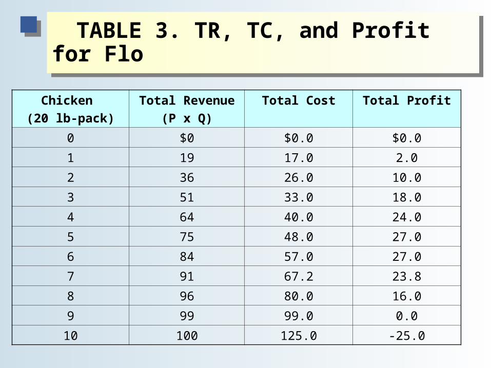
TABLE 3. TR, TC, and Profit for FloTABLE 3. TR, TC, and Profit for Flo
Chicken
(20 lb-pack)
Total Revenue
(P x Q)
Total Cost Total Profit
0 $0 $0.0 $0.0
1 19 17.0 2.0
2 36 26.0 10.0
3 51 33.0 18.0
4 64 40.0 24.0
5 75 48.0 27.0
6 84 57.0 27.0
7 91 67.2 23.8
8 96 80.0 16.0
9 99 99.0 0.0
10 100 125.0 -25.0
Copyright© 2006 Southwestern/Thomson Learning All rights reserved.
Total Profit: Keep Your Eye on the GoalTotal Profit: Keep Your Eye on the Goal
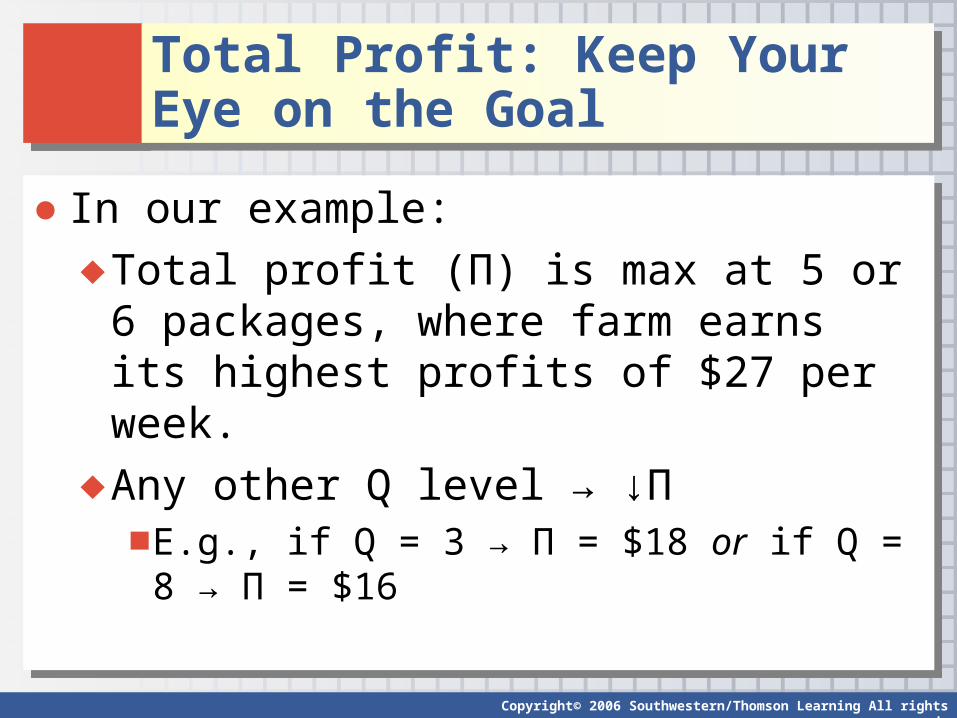
● In our example:
♦ Total profit (Π) is max at 5 or 6 packages, where farm earns its highest profits of $27 per week.
♦ Any other Q level → ↓Π■E.g., if Q = 3 → Π = $18 or if Q = 8 → Π = $16
● In our example:
♦ Total profit (Π) is max at 5 or 6 packages, where farm earns its highest profits of $27 per week.
♦ Any other Q level → ↓Π■E.g., if Q = 3 → Π = $18 or if Q = 8 → Π = $16
Copyright© 2006 Southwestern/Thomson Learning All rights reserved.
Marginal Analysis and Maximization of Total ProfitMarginal Analysis and Maximization of Total Profit
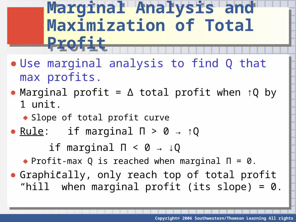
● Use marginal analysis to find Q that max profits.● Marginal profit = ∆ total profit when ↑Q by 1 unit.
♦ Slope of total profit curve
● Rule: if marginal Π > 0 → ↑Q
if marginal Π < 0 → ↓Q ♦ Profit-max Q is reached when marginal Π = 0.
● Graphically, only reach top of total profit “hill” when marginal profit (its slope) = 0.
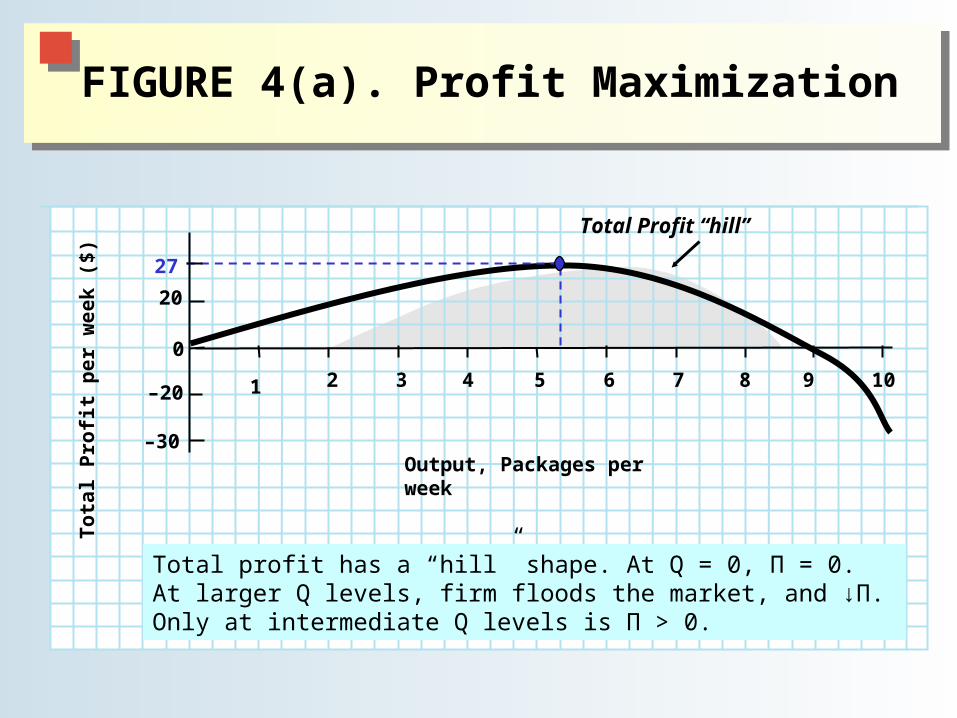
FIGURE 4(a). Profit MaximizationFIGURE 4(a). Profit Maximization
5
Output, Packages per week
10 9 8 7 6 4 3 2 1
–30
–20
0
20
27
To
tal
Pro
fit
pe
r w
ee
k (
$)
Total Profit “hill”
Total profit has a “hill” shape. At Q = 0, Π = 0. At larger Q levels, firm floods the market, and ↓Π. Only at intermediate Q levels is Π > 0.
Copyright© 2006 Southwestern/Thomson Learning All rights reserved.
Marginal Analysis and Maximization of Total ProfitMarginal Analysis and Maximization of Total Profit
● Like marginal Π, MR and MC can guide us to Q output where total profit is maximized.
● MR = slope of TR and MC = slope of TC ● Total profit is max when TR and TC are farthest apart.
♦ Occurs when their slopes are equal, so they are not growing closer together (Π↓) or growing further apart (Π↑).
● Rule: if MR > MC → Q
if MR < MC → Q♦ Profit maximizing Q is where MR = MC.
Copyright© 2006 Southwestern/Thomson Learning All rights reserved.
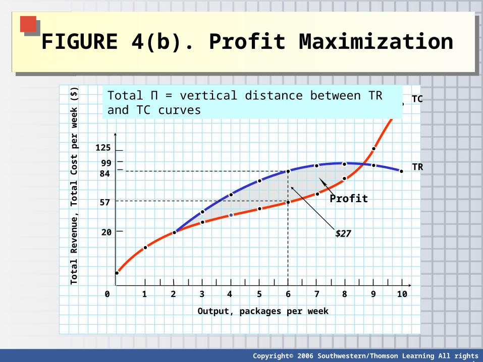
FIGURE 4(b). Profit MaximizationFIGURE 4(b). Profit Maximization
TC
TR
Profit
Output, packages per week
5
To
tal R
even
ue,
To
tal C
ost
per
wee
k ($
)
10 9 8 7 6 4 3 2 1 0
99 84
57
20 $27
125
Total Π = vertical distance between TR and TC curves
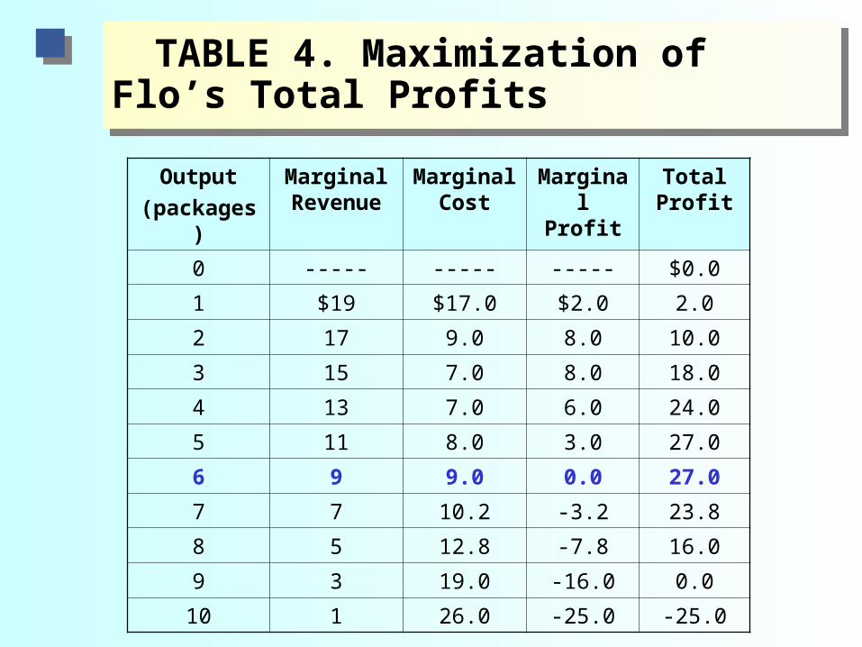
TABLE 4. Maximization of Flo’s Total Profits
TABLE 4. Maximization of Flo’s Total Profits
Output
(packages)
Marginal Revenue
Marginal Cost
Marginal Profit
Total Profit
0 ----- ----- ----- $0.0
1 $19 $17.0 $2.0 2.0
2 17 9.0 8.0 10.0
3 15 7.0 8.0 18.0
4 13 7.0 6.0 24.0
5 11 8.0 3.0 27.0
6 9 9.0 0.0 27.0
7 7 10.2 -3.2 23.8
8 5 12.8 -7.8 16.0
9 3 19.0 -16.0 0.0
10 1 26.0 -25.0 -25.0
Copyright© 2006 Southwestern/Thomson Learning All rights reserved.
Marginal Analysis and Maximization of Total ProfitMarginal Analysis and Maximization of Total Profit
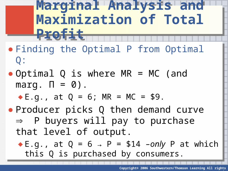
● Finding the Optimal P from Optimal Q:
● Optimal Q is where MR = MC (and marg. Π = 0).♦ E.g., at Q = 6; MR = MC = $9.
● Producer picks Q then demand curve P buyers will pay to purchase that level of output.♦ E.g., at Q = 6 → P = $14 –only P at which this Q is
purchased by consumers.
● Finding the Optimal P from Optimal Q:
● Optimal Q is where MR = MC (and marg. Π = 0).♦ E.g., at Q = 6; MR = MC = $9.
● Producer picks Q then demand curve P buyers will pay to purchase that level of output.♦ E.g., at Q = 6 → P = $14 –only P at which this Q is
purchased by consumers.
Copyright© 2006 Southwestern/Thomson Learning All rights reserved.
Logic of Marginal Analysis & MaximizationLogic of Marginal Analysis & Maximization
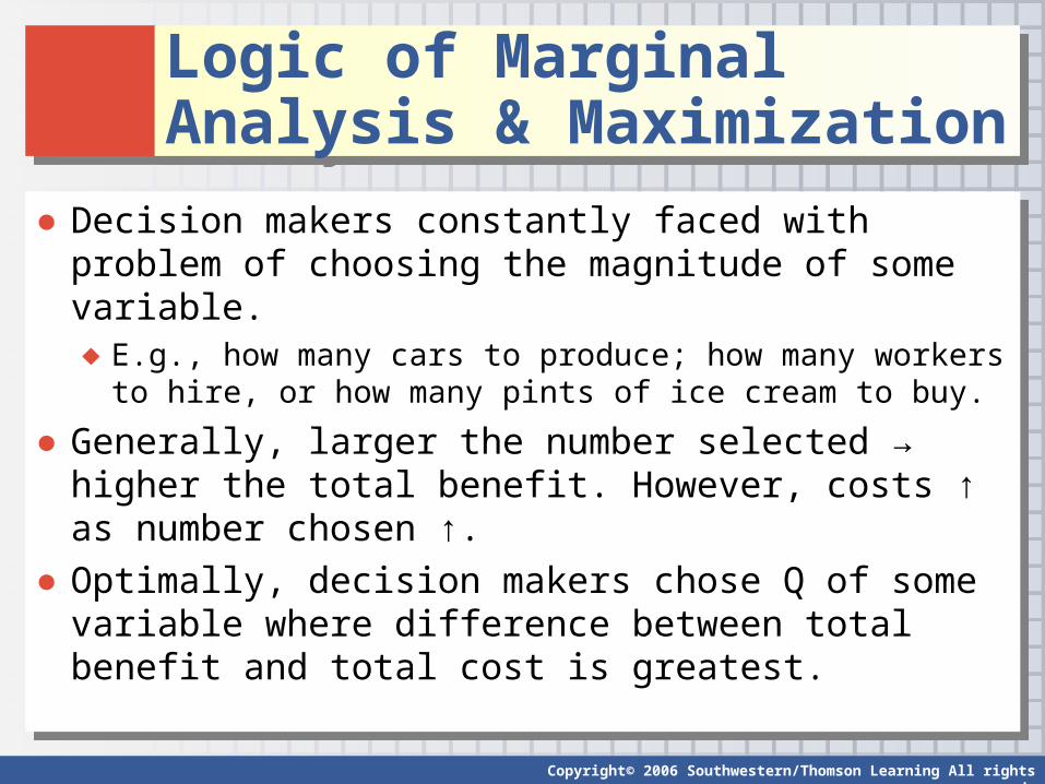
● Decision makers constantly faced with problem of choosing the magnitude of some variable. ♦ E.g., how many cars to produce; how many workers to hire, or
how many pints of ice cream to buy.
● Generally, larger the number selected → higher the total benefit. However, costs ↑ as number chosen ↑.
● Optimally, decision makers chose Q of some variable where difference between total benefit and total cost is greatest.
Copyright© 2006 Southwestern/Thomson Learning All rights reserved.
Logic of Marginal Analysis & MaximizationLogic of Marginal Analysis & Maximization
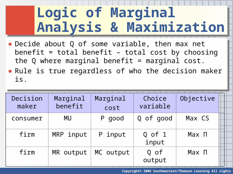
● Decide about Q of some variable, then max net benefit = total benefit – total cost by choosing the Q where marginal benefit = marginal cost.
● Rule is true regardless of who the decision maker is.
● Decide about Q of some variable, then max net benefit = total benefit – total cost by choosing the Q where marginal benefit = marginal cost.
● Rule is true regardless of who the decision maker is.
Decision maker
Marginal benefit
Marginal
cost
Choice variable
Objective
consumer MU P good Q of good Max CS
firm MRP input P input Q of 1 input Max Π
firm MR output MC output Q of output Max Π
Copyright© 2006 Southwestern/Thomson Learning All rights reserved.
Logic of Marginal Analysis & MaximizationLogic of Marginal Analysis & Maximization
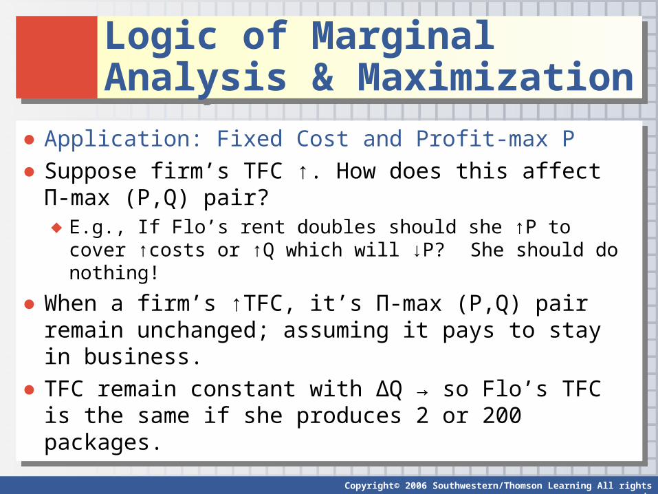
● Application: Fixed Cost and Profit-max P● Suppose firm’s TFC ↑. How does this affect Π-max
(P,Q) pair?♦ E.g., If Flo’s rent doubles should she ↑P to cover ↑costs or ↑Q
which will ↓P? She should do nothing!
● When a firm’s ↑TFC, it’s Π-max (P,Q) pair remain unchanged; assuming it pays to stay in business.
● TFC remain constant with ∆Q → so Flo’s TFC is the same if she produces 2 or 200 packages.
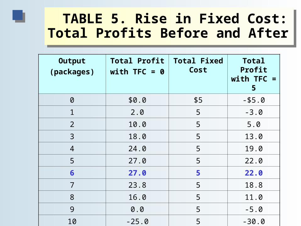
TABLE 5. Rise in Fixed Cost: Total Profits Before and After
TABLE 5. Rise in Fixed Cost: Total Profits Before and After
Output
(packages)
Total Profit
with TFC = 0
Total Fixed Cost
Total Profit with TFC = 5
0 $0.0 $5 -$5.0
1 2.0 5 -3.0
2 10.0 5 5.0
3 18.0 5 13.0
4 24.0 5 19.0
5 27.0 5 22.0
6 27.0 5 22.0
7 23.8 5 18.8
8 16.0 5 11.0
9 0.0 5 -5.0
10 -25.0 5 -30.0
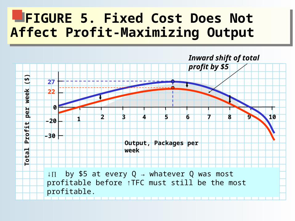
FIGURE 5. Fixed Cost Does Not Affect Profit-Maximizing Output
FIGURE 5. Fixed Cost Does Not Affect Profit-Maximizing Output
5
Output, Packages per week
10 9 8 7 6 4 3 2 1
–30
–20
0
22
27
To
tal
Pro
fit
pe
r w
ee
k (
$)
↓∏ by $5 at every Q → whatever Q was most profitable before ↑TFC must still be the most profitable.
Inward shift of total profit by $5
Copyright© 2006 Southwestern/Thomson Learning All rights reserved.
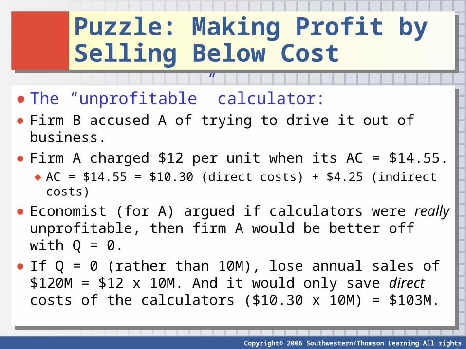
Puzzle: Making Profit by Selling Below CostPuzzle: Making Profit by Selling Below Cost
● The “unprofitable” calculator:● Firm B accused A of trying to drive it out of business.● Firm A charged $12 per unit when its AC = $14.55.
♦ AC = $14.55 = $10.30 (direct costs) + $4.25 (indirect costs)
● Economist (for A) argued if calculators were really unprofitable, then firm A would be better off with Q = 0.
● If Q = 0 (rather than 10M), lose annual sales of $120M = $12 x 10M. And it would only save direct costs of the calculators ($10.30 x 10M) = $103M.
Copyright© 2006 Southwestern/Thomson Learning All rights reserved.
Puzzle: Making Profit by Selling Below CostPuzzle: Making Profit by Selling Below Cost
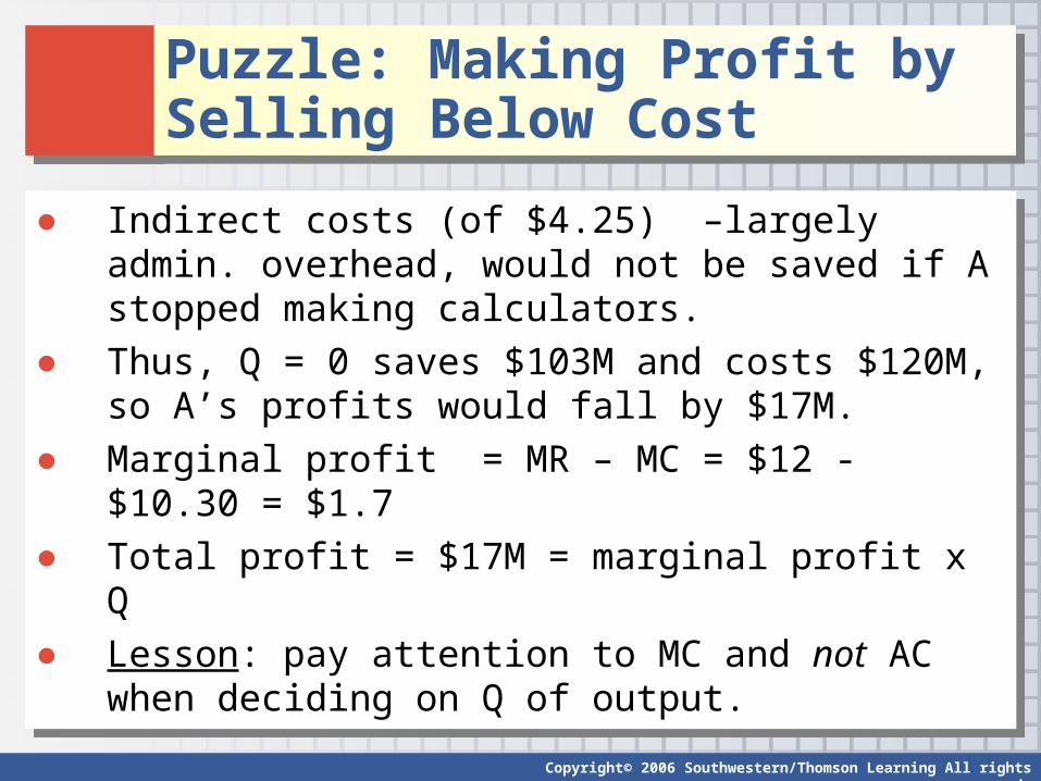
● Indirect costs (of $4.25) –largely admin. overhead, would not be saved if A stopped making calculators.
● Thus, Q = 0 saves $103M and costs $120M, so A’s profits would fall by $17M.
● Marginal profit = MR – MC = $12 - $10.30 = $1.7● Total profit = $17M = marginal profit x Q ● Lesson: pay attention to MC and not AC when
deciding on Q of output.