6 DoF SLAM using a ToF Camera:

The challenge of a continuously growing number of landmarks

Siegfried Hochdorfer and Christian Schlegel

University of Applied Sciences Ulm

Department of Computer Science, Prittwitzstr. 10, 89075 Ulm, Germany

email: {hochdorfer, schlegel}@hs-ulm.de

Abstract— Localization and mapping are fundamental prob-lems in service robotics since representations of the environmentand knowledge about the own pose significantly simplify theimplementation of a series of high-level applications.

ToF (time-of-flight) cameras are a relatively new kind ofsensors in robotics. They enable the real-time capture of thedistance and the grayscale information of a scene. Due to theincrease of the image resolution of ToF cameras, now highlevelcomputer vision algorithms for visual feature extraction (e.g.SIFT [1] or SURF [2]) can be applied to the captured images.These visual features combined with the corresponding distanceinformation give a full measurement of 3D landmarks.

An obvious problem to be solved is the continuously growingnumber of landmarks. So far, all ever seen landmarks are justaccumulated irrespective of their utility and the then requiredresources. Rather, one should keep only really useful landmarks,e.g. such that localization quality in the whole operational areais kept above a given threshold. In fact a lifelong runningSLAM approach is dependent on means to select and discardlandmarks. That is even more acute in case of feature-richsensor data as provided with high update rates by sensors likea ToF camera.

We run our SLAM approach in a real-world experimentwithin an indoor environment. The experiment was performedon a P3DX-platform equipped with a PMD CamCube 2.0 anda Xsens IMU.

I. INTRODUCTION

Localization and mapping are fundamental problems in

service robotics since representations of the environment and

knowledge about the own pose are crucial for a series of

high-level applications.

Especially in 3D SLAM, the requirements on the sen-

sors are high. ToF cameras provide a good performance

on capturing 3D scenes. They are able to simultaneously

capture distance and grayscale images with high frame rates.

The compact size and low power consumption makes them

suitable for use in robotics.

Service robots should be designed for life-long and ro-

bust operation in dynamic environments. However, SLAM

approaches typically just accumulate landmarks over time

and do not discard them anymore. Therefore, each newly

recognized landmark is added to the state vector which

results in a growth of the state vector size without an upper

bound. In case of bounded resources, one thus needs a

mechanism to keep only the best landmarks. The SLAM

problem thus needs to be extended such that one selects

those landmarks that ensure a certain localization quality

within the working environment of the service robot. The

other landmarks can be marked for deletion.

In this paper we present an approach to fuse ToF camera

data and 3D odometry for feature-based 6 DoF SLAM. The

focus lies on the validation of landmark measurements in

ToF images as well as on the data association part. The

problem of ever growing number of landmarks is handled by

a landmark rating and selection process. It selects landmarks

in such a way that they best cover the working environment

for localization purposes.

II. RELATED WORK

Well known sensors for 3D scene recognition are stereo-

vision systems. In weakly textured image regions it is not

possible to detect the necessary correspondences in both im-

ages for computing the distances. Beder [3] compares stereo

vision systems with a ToF camera for surface reconstruction

tasks. He shows that the ToF camera outperforms the stereo

vision system in case of distance measurements. Because the

resolution of the ToF camera is lower, he suggests to fuse

both kinds of cameras for surface reconstruction purposes.

Sabeti [4] proposes two Particle Filter based visual object

tracker. One is based on time-of-flight range image data and

the other one on 2D color camera data. He compares both

to identify the advantages and drawbacks of the systems.

The potential of ToF cameras in mobile robotics is de-

scribed by May [5]. First, he describes the influence of inte-

gration time and modulation frequency on the measurement

quality and how ToF cameras have to be calibrated. Then a

filter to determine inaccurate distance values is presented. In

[6] May uses a ToF camera for indoor SLAM based on depth

image registration. He discusses the error characteristics of

ToF cameras in detail and suggests, methods for camera

calibration. Several methods for registering real-world ToF

camera data using ICP based algorithms are explained.

Experiments in a indoor environment with a diagonal of

19.4m were reported. The trajectory forms a loop where 325

distance images are captured.

Prusak proposes an approach for pose estimation and map

building using ToF camera and 2D CCD camera [7]. A

combined Structure-from-Motion (SfM) and model-tracking

approach is used for selflocalization. The ToF camera image

is mapped into the 2D CCD image. The distance can be

determined by using the pixel by pixel correspondence for

The 2010 IEEE/RSJ International Conference on Intelligent Robots and Systems October 18-22, 2010, Taipei, Taiwan

978-1-4244-6676-4/10/$25.00 ©2010 IEEE 3981

every interest points. A KLT-tracker is used to track interest

points in the 2D CCD camera image. This set of interest

points is used for pose estimation.

An early approach using SIFT features as visual 3D land-

marks for SLAM is presented by Se [8]. The 3D landmarks

are extracted from stereo vision. Then the 3D landmark

measurements and the 2D odometry data are fused in a

Kalman Filter.

Landmark rating needs a measure for determining the

benefit of a landmark for localization purposes. In [9], the

observation region of a landmark together with the landmark

pose uncertainty is used for defining a measure for the

benefit of a landmark. DBSCAN clustering is used to identify

regions in the environment with a high landmark density.

A quality measure to compute the best landmark out

of a set of landmarks is also used by Dissanayake [10].

First, all landmarks are collected whose state changes in the

current step from visible to invisible. From this set only the

highest quality landmark is kept and all others are discarded.

Thus, the selected highest quality landmark is a single

representative for the set of previously visible landmarks.

However, selection of landmark representatives is based on

a local set of landmarks and thus depends on the exploration

path and the resulting visibility sequence. There is still no

global measure of landmark quality. Nevertheless, this is one

of the rare approaches addressing landmark deletion with

respect to a landmark’s use in terms of observability.

A fundamentally different approach is proposed by Stras-

dat [11]. The presented approach uses Monte-Carlo Rein-

forcement Learning to learn landmark selection policies that

optimize the navigation task. He demonstrates his approach

in two scenarios. The first is a single goal navigation task.

The second is a round-trip navigation task where subgoals

are visited more than once. Due to the complexity of the

learning algorithm and the number of training episodes,

it is not feasible to learn these policies during real-world

experimentation. Therefore, Strasdat recommends to learn

the policies in simulation.

III. METHOD

This section starts with the description of the overall

system. Then the used methods for the action and the sensing

step of the Extended Kalman Filter (EKF) are explained in

detail. Next, the approach used for the data association prob-

lem is presented. The data association problem is considered

as the major problem in robust feature-based EKF SLAM

approaches. Our proposed solution on handling the problem

of the ever growing number of landmarks during SLAM is

described at the end of this section.

The overall sequence of processing steps is shown in

figure 1. Wheel encoder data (2D odometry) together with

the inclinometer data are used to predict the relative 3D

pose change of the mobile robot. In the sensing step 3D

landmark measurements from the ToF camera are used.

SURF features extracted from the intensity image of the ToF

camera are used as salient and recognizable landmarks. The

SURF feature position in the intensity image together with

������������� ��

��������������

��������

������������������� � ���

����������

������� ������

�� ������� �����

������� �����

������ ������ ������� ��� ����������� �� ���� � ��

���������� ���� � ���� �!�∀ ���� ������ #

� ������ ������� �

Fig. 1. The overall system for 6 DoF SLAM

the distance measurement describes a full 3D measurement

in spherical coordinates. The observed SURF features are

compared with those from the previously observed ones in

the feature database. A SURF feature of the current scene

is considered as not matching an already known landmark,

if the comparison of the descriptors by a Chi-square test

is above a given threshold. In this case, the SURF feature

gets a new and unique identifier. Otherwise, the SURF

feature is considered as matching an already known landmark

and therefore gets the unique identifier of the recognized

landmark. Both, the predicted relative pose change (3D

odometry) and the data from the sensing step are then fused

in the EKF to estimate the 6 DoF pose of the mobile robot

and the 3D landmarks in the map.

A. Full 6 DoF EKF-based Bearing-Range SLAM

A tremendous amount of frameworks for SLAM algo-

rithms have been developed and published in the recent

years [12], [13]. Most of them provide basic algorithms

to solve the SLAM problem with probabilistic methods,

like Kalman Filter, Extended Kalman Filter and Particle

Filter. Our approach is based on the Range-Bearing SLAM

algorithm of Blanco [14]. This efficient implementation is

used in the Mobile Robot Programming Toolkit (MRPT) [13]

and has a complexity of O(N2). The state vector contains

the vehicle pose as well as all landmarks.

x = [xv, y1, y2, y3, . . . , yL]T (1)

The vehicle pose xv = [xv, yv, zv, φv, χv, ψv] is the position

in 3D Cartesian coordinates and the three orientation angles.

Every landmark yi = [xi, yi, zi] is represented by its 3D

coordinates in the map.

1) 3D Odometry: Typical wheel encoder based odometry

provides pose information in 2D (x, y, φ). The 3D odometry

approach presented in [15] and [16] extends the 2D odometry

to 3D by using inclinometer data for pitch (χ) and roll

(ψ). In case we use 3D landmarks, even ground vehicles

in indoor environments require 3D odometry due to ramps

or inclined planes. 3D odometry can be achieved by fusing

3982

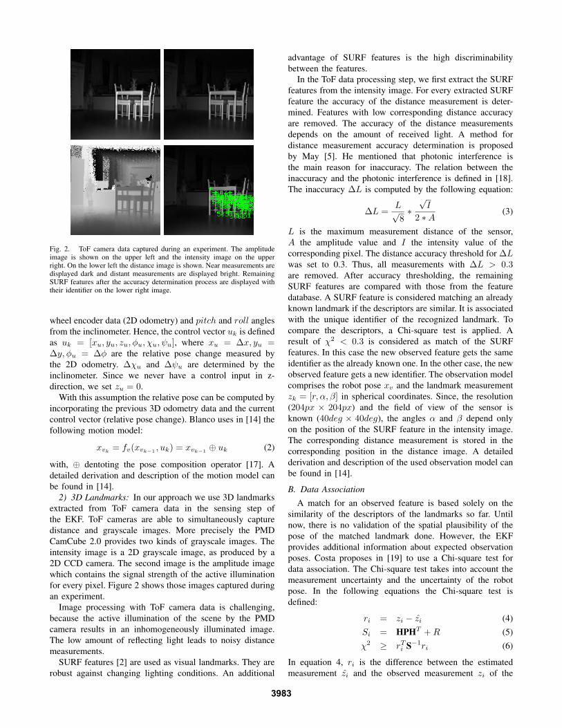
Fig. 2. ToF camera data captured during an experiment. The amplitudeimage is shown on the upper left and the intensity image on the upperright. On the lower left the distance image is shown. Near measurements aredisplayed dark and distant measurements are displayed bright. RemainingSURF features after the accuracy determination process are displayed withtheir identifier on the lower right image.

wheel encoder data (2D odometry) and pitch and roll angles

from the inclinometer. Hence, the control vector uk is defined

as uk = [xu, yu, zu, φu, χu, ψu], where xu = ∆x, yu =∆y, φu = ∆φ are the relative pose change measured by

the 2D odometry. ∆χu and ∆ψu are determined by the

inclinometer. Since we never have a control input in z-

direction, we set zu = 0.

With this assumption the relative pose can be computed by

incorporating the previous 3D odometry data and the current

control vector (relative pose change). Blanco uses in [14] the

following motion model:

xvk= fv(xvk−1

, uk) = xvk−1⊕ uk (2)

with, ⊕ dentoting the pose composition operator [17]. A

detailed derivation and description of the motion model can

be found in [14].

2) 3D Landmarks: In our approach we use 3D landmarks

extracted from ToF camera data in the sensing step of

the EKF. ToF cameras are able to simultaneously capture

distance and grayscale images. More precisely the PMD

CamCube 2.0 provides two kinds of grayscale images. The

intensity image is a 2D grayscale image, as produced by a

2D CCD camera. The second image is the amplitude image

which contains the signal strength of the active illumination

for every pixel. Figure 2 shows those images captured during

an experiment.

Image processing with ToF camera data is challenging,

because the active illumination of the scene by the PMD

camera results in an inhomogeneously illuminated image.

The low amount of reflecting light leads to noisy distance

measurements.

SURF features [2] are used as visual landmarks. They are

robust against changing lighting conditions. An additional

advantage of SURF features is the high discriminability

between the features.

In the ToF data processing step, we first extract the SURF

features from the intensity image. For every extracted SURF

feature the accuracy of the distance measurement is deter-

mined. Features with low corresponding distance accuracy

are removed. The accuracy of the distance measurements

depends on the amount of received light. A method for

distance measurement accuracy determination is proposed

by May [5]. He mentioned that photonic interference is

the main reason for inaccuracy. The relation between the

inaccuracy and the photonic interference is defined in [18].

The inaccuracy ∆L is computed by the following equation:

∆L =L√8∗

√I

2 ∗A (3)

L is the maximum measurement distance of the sensor,

A the amplitude value and I the intensity value of the

corresponding pixel. The distance accuracy threshold for ∆Lwas set to 0.3. Thus, all measurements with ∆L > 0.3are removed. After accuracy thresholding, the remaining

SURF features are compared with those from the feature

database. A SURF feature is considered matching an already

known landmark if the descriptors are similar. It is associated

with the unique identifier of the recognized landmark. To

compare the descriptors, a Chi-square test is applied. A

result of χ2 < 0.3 is considered as match of the SURF

features. In this case the new observed feature gets the same

identifier as the already known one. In the other case, the new

observed feature gets a new identifier. The observation model

comprises the robot pose xv and the landmark measurement

zk = [r, α, β] in spherical coordinates. Since, the resolution

(204px × 204px) and the field of view of the sensor is

known (40deg × 40deg), the angles α and β depend only

on the position of the SURF feature in the intensity image.

The corresponding distance measurement is stored in the

corresponding position in the distance image. A detailed

derivation and description of the used observation model can

be found in [14].

B. Data Association

A match for an observed feature is based solely on the

similarity of the descriptors of the landmarks so far. Until

now, there is no validation of the spatial plausibility of the

pose of the matched landmark done. However, the EKF

provides additional information about expected observation

poses. Costa proposes in [19] to use a Chi-square test for

data association. The Chi-square test takes into account the

measurement uncertainty and the uncertainty of the robot

pose. In the following equations the Chi-square test is

defined:

ri = zi − zi (4)

Si = HPHT +R (5)

χ2 ≥ rTi S−1ri (6)

In equation 4, ri is the difference between the estimated

measurement zi and the observed measurement zi of the

3983

landmark at index i. Si in equation 5 is the residual

covariance which is calculated by multiplying the system

covariance matrix with the Jacobian matrix H and the

transpose of the Jacobian matrix. After transforming the

covariance matrix into the measurement space the sensor

noise covariance matrix R is added. The Jacobian matrix

H is defined by the following equation

H =[

HR 0 . . . 0 HLi0 . . . 0

]

(7)

HR is the Jacobian of the transition model and HL is the

Jacobian of the observation model.

HR =∂f

∂x(8)

HL =∂h

∂x(9)

The motion model is denoted by f and the observation model

by h. The position of HL in H corresponds to the index of

the landmark in the state vector.

The right part of equation 6 describes the squared Ma-

halanobis distance [20]. For Gaussian distributions the Ma-

halanobis distance follows the Chi-square distribution. The

threshold for the Chi-Square test can be obtained from a Chi-

square table. Our system have three degrees-of-freedom. For

a confidence value of 90% to associate a measurement to

a landmark, the value for χ2 obtained from table lookup is

0.5844.

C. Landmark rating and Selection

The basic approach for landmark rating and selection is

presented in [9] and is integrated into the SLAM mechanism

(see figure 1). It can be used with all kinds of feature-based

EKF SLAM approaches. In previouse work the approach is

used in 3DoF SLAM here in the 6DoF case we only have

to extend the viewpoint location estimation from 2D to 3D.

The sensing step keeps track of the set of robot poses from

which a landmark has been observed so far. This provides the

basis for describing from where in the environment a certain

landmark is observable. This information provides then the

basis for evaluating the benefit of a landmark for localization

purposes. At every time step the approach determines the

map quality by calculating the viewpoint location and the

information content [10] of every landmark.

Removing a landmark from a region with high localization

support results in a small degradation of robot localization

quality only. Clustering algorithms are used to identify

regions in the environment with a high landmark density.

DBSCAN clustering [21] is especially suitable to determine

those regions. The algorithm typically constructs clusters

around local dense maxima, separated by regions of low

density. The algorithm does not need to know the number

of clusters in advance. A further advantage is the efficiency

(O(n∗log(n))) of the algorithm, equal to K-means [21] [22].

Removing landmarks within low density regions is critical.

Relocalization in these regions using those landmarks is

difficult. All viewpoint locations with a distance greater Epsto the Eps-neighborhood are considered as outliers. Outliers

are not part of a cluster and are thus never removed.

Fig. 3. The real world experiment is performed in the whole ZAFHlaboratory with a room-size of 15m × 9m.

������������

��������

��������

���������

Fig. 4. Pioneer 3DX platform equipped with embedded PC, Xsens IMUand ToF Camera (PMD CamCube 2.0)

IV. RESULTS

A. Experiment Setup

In this section, the results of the experiments are discussed

in detail. The performance is demonstrated within a standard

indoor environment by means of a real-world experiment.

The experiment has been performed in our lab with a size of

15m × 9m (see figure 3) partly with moving people in the

scene. We have not taken any precautions to avoid specular

reflections and surfaces with low reflectivity.

The experiments are performed on a P3DX-platform (see

figure 4) with the above described feature-based 3D SLAM

approach.

The resolution of the ToF camera (PMD CamCube 2.0)

is 204px × 204px and the field of view 40deg × 40deg.

Therefore the angular resolution is 0.1961deg. The repeata-

bility of distance measurements defined by the manufacturer

is < 3mm at 2m distance and 90% reflectivity. To measure

the pitch and roll inclination an Xsens IMU is used. The

static accuracy of the pitch and roll measurements is 0.5degand the dynamic accuracy 2deg RMS.

The parameters of the motion model are (0.03m)2/1merror for change in position (∆x,∆y,∆z) and

(3deg)2/360deg angular error for ∆φ ∆χ and ∆ψ.

The observation model uses (0.05m)2 as distance error (σ2

r )

and (0.3deg)2 as angular errors (σ2

α, σ2

β) of the landmark

observation.

The clustering algorithm constructs clusters around local

dense maxima, separated by regions of low density. All

viewpoint locations with a distance greater Eps = 0.2mto the Eps-neighborhood belong to a cluster. Every cluster

needs at least 4 viewpoint locations. Otherwise the viewpoint

3984

x [m]

y [m

]

1 2 3 4 5 6 7 8 9 10 11 12 13 14 15

1

2

3

4

5

6

7

8

9

10

estimated robot trajectory

ground truth

robot pose

2σ covariance ellipse

Fig. 5. The estimated trajectory in the environment is plotted with a blueline. For visualization purposes, we project the 3D robot pose onto the 2Dplane and place a floor plan in the background. The gray objects are tables.The yellow triangles represent the robot with the 2σ covariance ellipse (red).For these robot poses the corresponding ground truth positions are markedwith a black cross.

locations are considered as outliers.

B. Localization Quality

The localization quality directly depends on the quality

of the landmarks and their distribution over the operational

area. As can be seen from figures 5, 7 and 8 the achieved

overall localization quality is still within a range suitable

for service robotic tasks. Figure 8 illustrates the localization

error against ground truth measurements. The error value

plotted there is the Euclidean distance from the ground truth

measurement to the mean of the robots state estimation. Due

to the lack of GPS/DGPS in indoor environments, it is quite

hard to get the ground truth position of the robot. We solve

the problem of determining the ground truth position by

measuring manually the distance from the robot towards two

a priori known coordinates in the environment with a Bosch

Digital Laser Rangefinder (DLE 150). The 2σ value of our

ground truth poses is [0.06m2, 0.04m2].

The trajectory shown in figure 5 contains 1401 time steps

and has a length of approximately 124m with an average step

width of 0.09m. During the run, the robot closes multiple

loops with a length of approximately 6m to 17m each. The

result after the experiment is a consistent map and a high

positioning accuracy of the robot.

Figure 6 shows all map objects at time step 1401. The

landmarks in the state vector are plotted with the corre-

sponding 2σ covariance ellipsoid (blue). The red colored

ellipsoid visualizes the robot pose covariance (2σ). The robot

coordinate system origin is represented as a X,Y,Z (red,

green, blue) 3D corner. This marks the start position of the

experiment.

In Figure 7 uncertainty of the robot pose estimation is

visualized by plotting the eigenvalues of the robot position

covariance matrix during the complete run. The plot in the

figure clearly indicates the decrease of uncertainty after every

loop closing.

A common method to evaluate the SLAM approach is

Fig. 6. 3D scene of the estimated map at time step 1401 with robot pose,the corresponding 2σ covariance ellipsoid (red) and the landmarks withtheir 2σ covariance ellipsoid (blue). The three arrows designate the originof the robot coordinate system (x,y,z : red, green,blue). Every square on theground plane is of size 1m × 1m.

0 500 1000 1500

0.05

0.1

0.15

0.2

0.25

0.3

0.35

0.4

0.45

time [steps]

eig

en v

alu

e [m

2]

eigen value λ

1

eigen value λ2

eigen value λ3

Fig. 7. Eigenvalues of the robot position covariance matrix during the run.

0 500 1000 15000

0.1

0.2

0.3

0.4

0.5

time [steps]

err

or

[m]

Fig. 8. Localization error against ground truth.

the comparison of the estimated robot pose against ground

truth. During the experiment, we made 28 ground truth

measurements. The Euclidean distance from the estimated

robot pose to the ground truth measurement is shown in

figure 8. If we compare the localization error in figure 8 with

the estimated pose uncertainty in figure 7, we can see that

time steps with a large distance to ground truth correlates

with the time steps with a high pose uncertainty. After

loop closing, the localization error and the pose uncertainty

decrease.

C. Landmark coverage quality

The landmark coverage of the environment is, as pre-

viously mentioned, a crucial factor for the relocalization

3985

3986