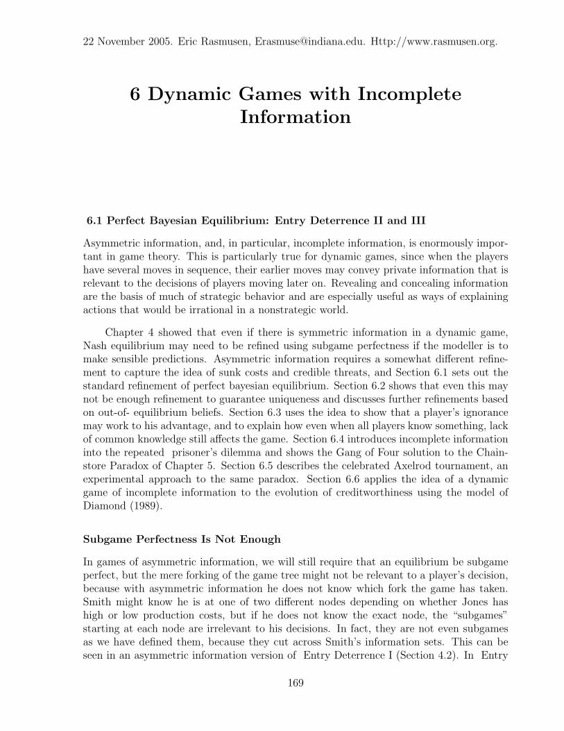
22 November 2005. Eric Rasmusen, Erasmuse@indiana.edu. Http://www.rasmusen.org.

6 Dynamic Games with IncompleteInformation

6.1 Perfect Bayesian Equilibrium: Entry Deterrence II and III

Asymmetric information, and, in particular, incomplete information, is enormously impor-tant in game theory. This is particularly true for dynamic games, since when the playershave several moves in sequence, their earlier moves may convey private information that isrelevant to the decisions of players moving later on. Revealing and concealing informationare the basis of much of strategic behavior and are especially useful as ways of explainingactions that would be irrational in a nonstrategic world.

Chapter 4 showed that even if there is symmetric information in a dynamic game,Nash equilibrium may need to be refined using subgame perfectness if the modeller is tomake sensible predictions. Asymmetric information requires a somewhat different refine-ment to capture the idea of sunk costs and credible threats, and Section 6.1 sets out thestandard refinement of perfect bayesian equilibrium. Section 6.2 shows that even this maynot be enough refinement to guarantee uniqueness and discusses further refinements basedon out-of- equilibrium beliefs. Section 6.3 uses the idea to show that a player’s ignorancemay work to his advantage, and to explain how even when all players know something, lackof common knowledge still affects the game. Section 6.4 introduces incomplete informationinto the repeated prisoner’s dilemma and shows the Gang of Four solution to the Chain-store Paradox of Chapter 5. Section 6.5 describes the celebrated Axelrod tournament, anexperimental approach to the same paradox. Section 6.6 applies the idea of a dynamicgame of incomplete information to the evolution of creditworthiness using the model ofDiamond (1989).

Subgame Perfectness Is Not Enough

In games of asymmetric information, we will still require that an equilibrium be subgameperfect, but the mere forking of the game tree might not be relevant to a player’s decision,because with asymmetric information he does not know which fork the game has taken.Smith might know he is at one of two different nodes depending on whether Jones hashigh or low production costs, but if he does not know the exact node, the “subgames”starting at each node are irrelevant to his decisions. In fact, they are not even subgamesas we have defined them, because they cut across Smith’s information sets. This can beseen in an asymmetric information version of Entry Deterrence I (Section 4.2). In Entry

169

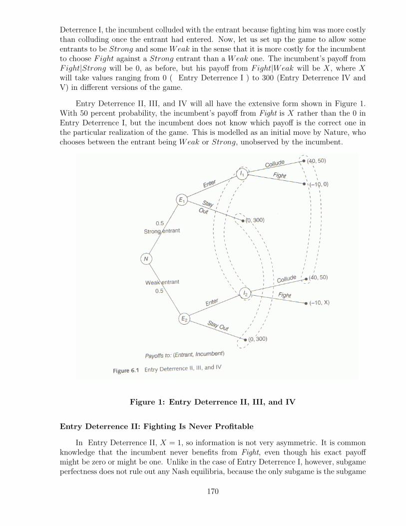
Deterrence I, the incumbent colluded with the entrant because fighting him was more costlythan colluding once the entrant had entered. Now, let us set up the game to allow someentrants to be Strong and some Weak in the sense that it is more costly for the incumbentto choose Fight against a Strong entrant than a Weak one. The incumbent’s payoff fromFight|Strong will be 0, as before, but his payoff from Fight|Weak will be X, where Xwill take values ranging from 0 ( Entry Deterrence I ) to 300 (Entry Deterrence IV andV) in different versions of the game.

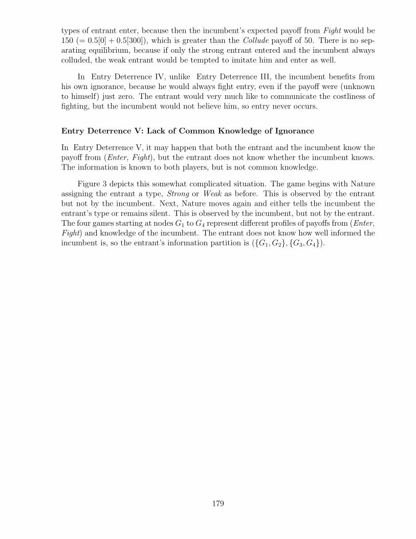
Entry Deterrence II, III, and IV will all have the extensive form shown in Figure 1.With 50 percent probability, the incumbent’s payoff from Fight is X rather than the 0 inEntry Deterrence I, but the incumbent does not know which payoff is the correct one inthe particular realization of the game. This is modelled as an initial move by Nature, whochooses between the entrant being Weak or Strong, unobserved by the incumbent.

Figure 1: Entry Deterrence II, III, and IV

Entry Deterrence II: Fighting Is Never Profitable

In Entry Deterrence II, X = 1, so information is not very asymmetric. It is commonknowledge that the incumbent never benefits from Fight, even though his exact payoffmight be zero or might be one. Unlike in the case of Entry Deterrence I, however, subgameperfectness does not rule out any Nash equilibria, because the only subgame is the subgame

170

starting at node N , which is the entire game. A subgame cannot start at nodes E1 or E2,because neither of those nodes are singletons in the information partitions. Thus, theimplausible Nash equilibrium, (Stay Out, Fight), escapes elimination by a technicality.

The equilibrium concept needs to be refined in order to eliminate the implausibleequilibrium. Two general approaches can be taken: either introduce small “trembles” intothe game, or require that strategies be best responses given rational beliefs. The firstapproach takes us to the “trembling hand-perfect” equilibrium, while the second takes usto the “perfect bayesian” and “sequential” equilibrium. The results are similar whicheverapproach is taken.

Trembling-Hand Perfectness

Trembling-hand perfectness is an equilibrium concept introduced by Selten (1975) accordingto which a strategy that is to be part of an equilibrium must continue to be optimal for theplayer even if there is a small chance that the other player will pick an out-of-equilibriumaction (i.e., that the other player’s hand will “tremble”).

Trembling-hand perfectness is defined for games with finite action sets as follows.

The strategy profile s∗ is a trembling-hand perfect equilibrium if for any ε there is avector of positive numbers δ1, . . . , δn ∈ [0, 1] and a vector of completely mixed strategiesσ1, . . . σn such that the perturbed game where every strategy is replaced by (1− δi)si + δiσi

has a Nash equilibrium in which every strategy is within distance ε of s∗.

Every trembling-hand perfect equilibrium is subgame perfect; indeed, Section 4.1 jus-tified subgame perfectness using a tremble argument. Unfortunately, it is often hard totell whether a strategy profile is trembling- hand perfect, and the concept is undefined forgames with continuous strategy spaces because it is hard to work with mixtures of a con-tinuum (see note N3.1). Moreover, the equilibrium depends on which trembles are chosen,and deciding why one tremble should be more common than another may be difficult.

Perfect Bayesian Equilibrium and Sequential Equilibrium

The second approach to asymmetric information, introduced by Kreps & Wilson (1982b)in the spirit of Harsanyi (1967), is to start with prior beliefs, common to all players, thatspecify the probabilities with which Nature chooses the types of the players at the beginningof the game. Some of the players observe Nature’s move and update their beliefs, whileother players can update their beliefs only by deductions they make from observing theactions of the informed players.

The deductions used to update beliefs are based on the actions specified by the equilib-rium. When players update their beliefs, they assume that the other players are followingthe equilibrium strategies, but since the strategies themselves depend on the beliefs, anequilibrium can no longer be defined based on strategies alone. Under asymmetric infor-mation, an equilibrium is a strategy profile and a set of beliefs such that the strategies arebest responses. The profile of beliefs and strategies is called an assessment by Kreps andWilson.

171

On the equilibrium path, all that the players need to update their beliefs are theirpriors and Bayes’ s Rule, but off the equilibrium path this is not enough. Suppose thatin equilibrium, the entrant always enters. If for whatever reason the impossible happensand the entrant stays out, what is the incumbent to think about the probability that theentrant is weak? Bayes’ s Rule does not help, because when Prob(data) = 0, which is thecase for data such as Stay Out which is never observed in equilibrium, the posterior beliefcannot be calculated using Bayes’ s Rule. From section 2.4,

Prob(Weak|Stay Out) =Prob(Stay Out|Weak)Prob(Weak)

Prob(Stay Out). (1)

The posterior Prob(Weak|Stay Out) is undefined, because (1) requires dividing by zero.

A natural way to define equilibrium is as a strategy profile consisting of best responsesgiven that equilibrium beliefs follow Bayes’ s Rule and out-of- equilibrium beliefs follow aspecified pattern that does not contradict Bayes’ s Rule.

A perfect bayesian equilibrium is a strategy profile s and a set of beliefs µ such that ateach node of the game:

(1) The strategies for the remainder of the game are Nash given the beliefs and strategiesof the other players.(2) The beliefs at each information set are rational given the evidence appearing thus far inthe game (meaning that they are based, if possible, on priors updated by Bayes’ s Rule, giventhe observed actions of the other players under the hypothesis that they are in equilibrium).

Kreps & Wilson (1982b) use this idea to form their equilibrium concept of sequen-tial equilibrium, but they impose a third condition, defined only for games with discretestrategies, to restrict beliefs a little further:

(3) The beliefs are the limit of a sequence of rational beliefs, i.e., if (µ∗, s∗) is the equi-librium assessment, then some sequence of rational beliefs and completely mixed strategiesconverges to it:

(µ∗, s∗) = Limn→∞(µn, sn) for some sequence (µn, sn) in {µ, s}.

Condition (3) is quite reasonable and makes sequential equilibrium close to trembling-hand perfect equilibrium, but it adds more to the concept’s difficulty than to its usefulness.If players are using the sequence of completely mixed strategies sn, then every action istaken with some positive probability, so Bayes’Rule can be applied to form the beliefs µn

after any action is observed. Condition (3) says that the equilibrium assessment has to bethe limit of some such sequence (though not of every such sequence). For the rest of thebook we will use perfect bayesian equilibrium and dispense with condition (3), although itusually can be satisfied.

Sequential equilibria are always subgame perfect (condition (1) takes care of that).Every trembling-hand perfect equilibrium is a sequential equilibrium, and “almost every”sequential equilibrium is trembling hand perfect. Every sequential equilibrium is perfectbayesian, but not every perfect bayesian equilibrium is sequential.

172

Back to Entry Deterrence II

Armed with the concept of the perfect bayesian equilibrium, we can find a sensible equi-librium for Entry Deterrence II .

Entrant: Enter|Weak, Enter|StrongIncumbent: ColludeBeliefs: Prob( Strong| Stay Out) = 0.4

In this equilibrium the entrant enters whether he is Weak or Strong. The incumbent’sstrategy is Collude, which is not conditioned on Nature’s move, since he does not observeit. Because the entrant enters regardless of Nature’s move, an out-of-equilibrium belief forthe incumbent if he should observe Stay Out must be specified, and this belief is arbitrarilychosen to be that the incumbent’s subjective probability that the entrant is Strong is 0.4given his observation that the entrant deviated by choosing Stay Out. Given this strategyprofile and out-of-equilibrium belief, neither player has incentive to change his strategy.

There is no perfect bayesian equilibrium in which the entrant chooses Stay Out. Fightis a bad response even under the most optimistic possible belief, that the entrant is Weakwith probability 1. Notice that perfect bayesian equilibrium is not defined structurally, likesubgame perfectness, but rather in terms of optimal responses. This enables it to comecloser to the economic intuition which we wish to capture by an equilibrium refinement.

Finding the perfect bayesian equilibrium of a game, like finding the Nash equilibrium,requires intelligence. Algorithms are not useful. To find a Nash equilibrium, the modellerthinks about his game, picks a plausible strategy profile, and tests whether the strategiesare best responses to each other. To make it a perfect bayesian equilibrium, he noteswhich actions are never taken in equilibrium and specifies the beliefs that players use tointerpret those actions. He then tests whether each player’s strategies are best responsesgiven his beliefs at each node, checking in particular whether any player would like to takean out-of-equilibrium action in order to set in motion the other players’ out-of-equilibriumbeliefs and strategies. This process does not involve testing whether a player’s beliefs arebeneficial to the player, because players do not choose their own beliefs; the priors andout-of-equilibrium beliefs are exogenously specified by the modeller.

One might wonder why the beliefs have to be specified in Entry Deterrence II. Doesnot the game tree specify the probability that the entrant is Weak? What differencedoes it make if the entrant stays out? Admittedly, Nature does choose each type withprobability 0.5, so if the incumbent had no other information than this prior, that wouldbe his belief. But the entrant’s action might convey additional information. The conceptof perfect bayesian equilibrium leaves the modeller free to specify how the players formbeliefs from that additional information, so long as the beliefs do not violate Bayes’ Rule.(A technically valid choice of beliefs by the modeller might still be met with scorn, though,as with any silly assumption. ) Here, the equilibrium says that if the entrant stays out,the incumbent believes he is Strong with probability 0.4 and Weak with probability 0.6,beliefs that are arbitrary but do not contradict Bayes’ s Rule.

In Entry Deterrence II the out-of-equilibrium beliefs do not and should not matter.

173

If the entrant chooses Stay Out, the game ends, so the incumbent’s beliefs are irrelevant.Perfect bayesian equilibrium was only introduced as a way out of a technical problem. Inthe next section, however, the precise out-of- equilibrium beliefs will be crucial to whichstrategy profiles are equilibria.

6.2 Refining Perfect Bayesian Equilibrium: The PhD Admissions Game

Entry Deterrence III: Fighting Is Sometimes Profitable

In Entry Deterrence III, assume that X = 60, not X = 1. This means that fighting is moreprofitable for the incumbent than collusion if the entrant is Weak. As before, the entrantknows if he is Weak, but the incumbent does not. Retaining the prior after observingout- of-equilibrium actions, which in this game is Prob(Strong) = 0.5, is a convenient wayto form beliefs that is called passive conjectures. The following is a perfect bayesianequilibrium which uses passive conjectures.

A plausible pooling equilibrium for Entry Deterrence IIIEntrant: Enter|Weak, Enter|StrongIncumbent: Collude, Out-of-equilibrium beliefs: Prob(Strong| Stay Out) = 0.5

In choosing whether to enter, the entrant must predict the incumbent’s behavior. Ifthe probability that the entrant is Weak is 0.5, the expected payoff to the incumbentfrom choosing Fight is 30 (= 0.5[0] + 0.5[60]), which is less than the payoff of 50 fromCollude. The incumbent will collude, so the entrant enters. The entrant may know thatthe incumbent’s payoff is actually 60, but that is irrelevant to the incumbent’s behavior.

The out-of-equilibrium belief does not matter to this first equilibrium, although it willin other equilibria of the same game. Although beliefs in a perfect bayesian equilibriummust follow Bayes’ s Rule, that puts very little restriction on how players interpret out-of-equilibrium behavior. Out-of- equilibrium behavior is “impossible,” so when it does occurthere is no obvious way the player should react. Some beliefs may seem more reasonablethan others, however, and Entry Deterrence III has another equilibrium that requires lessplausible beliefs off the equilibrium path.

An implausible equilibrium for Entry Deterrence IIIEntrant: Stay Out|Weak, Stay Out|StrongIncumbent: Fight, Out-of-equilibrium beliefs: Prob(Strong|Enter) = 0.1

This is an equilibrium because if the entrant were to deviate and enter, the incumbentwould calculate his payoff from fighting to be 54 (= 0.1[0] + 0.9[60]), which is greater thanthe Collude payoff of 50. The entrant would therefore stay out.

The beliefs in the implausible equilibrium are different and less reasonable than in theplausible equilibrium. Why should the incumbent believe that weak entrants would enter

174

mistakenly nine times as often as strong entrants? The beliefs do not violate Bayes’ s Rule,but they have no justification.

The reasonableness of the beliefs is important because if the incumbent uses passiveconjectures, the implausible equilibrium breaks down. With passive conjectures, the in-cumbent would want to change his strategy to Collude, because the expected payoff fromFight would be less than 50. The implausible equilibrium is less robust with respect tobeliefs than the plausible equilibrium, and it requires beliefs that are harder to justify.

Even though dubious outcomes may be perfect bayesian equilibria, the concept doeshave some bite, ruling out other dubious outcomes. There does not, for example, exist anequilibrium in which the entrant enters only if he is Strong and stays out if he is Weak(called a “separating equilibrium” because it separates out different types of players). Suchan equilibrium would have to look like this:

A conjectured separating equilibrium for Entry Deterrence IIIEntrant: Stay Out|Weak, Enter|StrongIncumbent: Collude

No out-of-equilibrium beliefs are specified for the conjectures in the separating equi-librium because there is no out-of-equilibrium behavior about which to specify them. Sincethe incumbent might observe either Stay out or Enter in equilibrium, the incumbent willalways use Bayes’ s Rule to form his beliefs. He will believe that an entrant who staysout must be weak and an entrant who enters must be strong. This conforms to the ideabehind Nash equilibrium that each player assumes that the other follows the equilibriumstrategy, and then decides how to reply. Here, the incumbent’s best response, given hisbeliefs, is Collude|Enter, so that is the second part of the proposed equilibrium. But thiscannot be an equilibrium, because the entrant would want to deviate. Knowing that entrywould be followed by collusion, even the weak entrant would enter. So there cannot be anequilibrium in which the entrant enters only when strong.

The PhD Admissions Game

Passive conjectures may not always be the most satisfactory belief, as the next exampleshows. Suppose that a university knows that 90 percent of the population hate economicsand would be unhappy in its PhD program, and 10 percent love economics and woulddo well. In addition, it cannot observe the applicant’s type. If the university rejects anapplication, its payoff is 0 and the applicant’s is −1 because of the trouble needed to apply.If the university accepts the application of someone who hates economics, the payoffs ofboth university and student are −10, but if the applicant loves economics, the payoffsare +20 for each player. Figure 2 shows this game in extensive form. The populationproportions are represented by a node at which Nature chooses the student to be a Loveror Hater of economics.

175

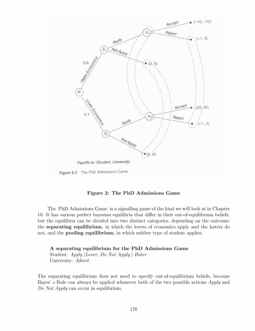
Figure 2: The PhD Admissions Game

The PhD Admissions Game is a signalling game of the kind we will look at in Chapter10. It has various perfect bayesian equilibria that differ in their out-of-equilibrium beliefs,but the equilibria can be divided into two distinct categories, depending on the outcome:the separating equilibrium, in which the lovers of economics apply and the haters donot, and the pooling equilibrium, in which neither type of student applies.

A separating equilibrium for the PhD Admissions GameStudent: Apply |Lover, Do Not Apply | HaterUniversity: Admit

The separating equilibrium does not need to specify out-of-equilibrium beliefs, becauseBayes’ s Rule can always be applied whenever both of the two possible actions Apply andDo Not Apply can occur in equilibrium.

176

A pooling equilibrium for the PhD Admissions GameStudent: Do Not Apply |Lover, Do Not Apply |HaterUniversity: Reject, Out-of-equilibrium beliefs: Prob(Hater |Apply) = 0.9 (pas-sive conjectures)

The pooling equilibrium is supported by passive conjectures. Both types of students refrainfrom applying because they believe correctly that they would be rejected and receive apayoff of −1; and the university is willing to reject any student who foolishly applied,believing that he is a Hater with 90 percent probability.

Because the perfect bayesian equilibrium concept imposes no restrictions on out-of-equilibrium beliefs, economists have come up with a variety of exotic refinements of theequilibrium concept. Let us consider whether various alternatives to passive conjectureswould support the pooling equilibrium in PhD Admissions.

Passive Conjectures. Prob(Hater|Apply) = 0.9

This is the belief specified above, under which out-of-equilibrium behavior leaves beliefsunchanged from the prior. The argument for passive conjectures is that the student’sapplication is a mistake, and that both types are equally likely to make mistakes, althoughHaters are more common in the population. This supports the pooling equilibrium.

The Intuitive Criterion. Prob(Hater|Apply) = 0

Under the Intuitive Criterion of Cho & Kreps (1987), if there is a type of informedplayer who could not benefit from the out-of-equilibrium action no matter what beliefs wereheld by the uninformed player, the uninformed player’s belief must put zero probabilityon that type. Here, the Hater could not benefit from applying under any possible beliefsof the university, so the university puts zero probability on an applicant being a Hater.This argument will not support the pooling equilibrium, because if the university holdsthis belief, it will want to admit anyone who applies.

Complete Robustness. Prob(Hater|Apply) = m, 0 ≤ m ≤ 1

Under this approach, the equilibrium strategy profile must consist of responses that arebest, given any and all out-of-equilibrium beliefs. Our equilibrium for Entry Deterrence IIsatisfied this requirement. Complete robustness rules out a pooling equilibrium in the PhDAdmissions Game, because a belief like m = 0 makes accepting applicants a best response,in which case only the Lover will apply. A useful first step in analyzing conjectured poolingequilibria is to test whether they can be supported by extreme beliefs such as m = 0 andm = 1.

An Ad Hoc Specification. Prob(Hater|Apply) = 1

Sometimes the modeller can justify beliefs by the circumstances of the particular game.Here, one could argue that anyone so foolish as to apply knowing that the university would

177

reject them could not possibly have the good taste to love economics. This supports thepooling equilibrium also.

An alternative approach to the problem of out-of-equilibrium beliefs is to removeits origin by building a model in which every outcome is possible in equilibrium becausedifferent types of players take different equilibrium actions. In the PhD Admissions Game,we could assume that there are a few students who both love economics and actuallyenjoy writing applications. Those students would always apply in equilibrium, so therewould never be a pure pooling equilibrium in which nobody applied, and Bayes’ s Rulecould always be used. In equilibrium, the university would always accept someone whoapplied, because applying is never out-of-equilibrium behavior and it always indicates thatthe applicant is a Lover. This approach is especially attractive if the modeller takes thepossibility of trembles literally, instead of just using it as a technical tool.

The arguments for different kinds of beliefs can also be applied to Entry Deterrence III,which had two different pooling equilibria and no separating equilibrium. We used passiveconjectures in the “plausible” equilibrium. The intuitive criterion would not restrict beliefsat all, because both types would enter if the incumbent’s beliefs were such as to make himcollude, and both would stay out if they made him fight. Complete robustness would ruleout as an equilibrium the strategy profile in which the entrant stays out regardless of type,because the optimality of staying out depends on the beliefs. It would support the strategyprofile in which the entrant enters and out-of-equilibrium beliefs do not matter.

6.3 The Importance of Common Knowledge: Entry Deterrence IV and V

To demonstrate the importance of common knowledge, let us consider two more versionsof Entry Deterrence. We will use passive conjectures in both. In Entry Deterrence III, theincumbent was hurt by his ignorance. Entry Deterrence IV will show how he can benefitfrom it, and Entry Deterrence V will show what can happen when the incumbent has thesame information as the entrant but the information is not common knowledge.

Entry Deterrence IV: The Incumbent Benefits from Ignorance

To construct Entry Deterrence IV, let X = 300 in Figure 1, so fighting is even moreprofitable than in Entry Deterrence III but the game is otherwise the same: the entrantknows his type, but the incumbent does not. The following is the unique perfect bayesianequilibrium in pure strategies.1

Equilibrium for Entry Deterrence IVEntrant: Stay Out |Weak, Stay Out |StrongIncumbent: Fight, Out-of-equilibrium beliefs: Prob(Strong|Enter) = 0.5 (pas-sive conjectures)

This equilibrium can be supported by other out-of-equilibrium beliefs, but no equilib-rium is possible in which the entrant enters. There is no pooling equilibrium in which both

1There exists a plausible mixed-strategy equilibrium too: Entrant: Enter if Strong, Enter with proba-bility m = 0.2 if Weak; Incumbent: Collude with probability n = 0.2. The payoff from this is only 150, soif the equilibrium were one in mixed strategies, ignorance would not help.

178

types of entrant enter, because then the incumbent’s expected payoff from Fight would be150 (= 0.5[0] + 0.5[300]), which is greater than the Collude payoff of 50. There is no sep-arating equilibrium, because if only the strong entrant entered and the incumbent alwayscolluded, the weak entrant would be tempted to imitate him and enter as well.

In Entry Deterrence IV, unlike Entry Deterrence III, the incumbent benefits fromhis own ignorance, because he would always fight entry, even if the payoff were (unknownto himself) just zero. The entrant would very much like to communicate the costliness offighting, but the incumbent would not believe him, so entry never occurs.

Entry Deterrence V: Lack of Common Knowledge of Ignorance

In Entry Deterrence V, it may happen that both the entrant and the incumbent know thepayoff from (Enter, Fight), but the entrant does not know whether the incumbent knows.The information is known to both players, but is not common knowledge.

Figure 3 depicts this somewhat complicated situation. The game begins with Natureassigning the entrant a type, Strong or Weak as before. This is observed by the entrantbut not by the incumbent. Next, Nature moves again and either tells the incumbent theentrant’s type or remains silent. This is observed by the incumbent, but not by the entrant.The four games starting at nodes G1 to G4 represent different profiles of payoffs from (Enter,Fight) and knowledge of the incumbent. The entrant does not know how well informed theincumbent is, so the entrant’s information partition is ({G1, G2}, {G3, G4}).

179

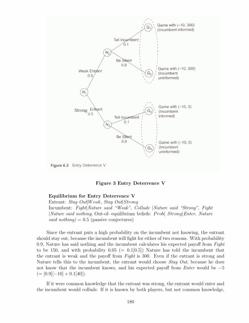
Figure 3 Entry Deterrence V

Equilibrium for Entry Deterrence VEntrant: Stay Out|Weak, Stay Out|StrongIncumbent: Fight|Nature said “Weak”, Collude |Nature said “Strong”, Fight|Nature said nothing, Out-of- equilibrium beliefs: Prob( Strong|Enter, Naturesaid nothing) = 0.5 (passive conjectures)

Since the entrant puts a high probability on the incumbent not knowing, the entrantshould stay out, because the incumbent will fight for either of two reasons. With probability0.9, Nature has said nothing and the incumbent calculates his expected payoff from Fightto be 150, and with probability 0.05 (= 0.1[0.5]) Nature has told the incumbent thatthe entrant is weak and the payoff from Fight is 300. Even if the entrant is strong andNature tells this to the incumbent, the entrant would choose Stay Out, because he doesnot know that the incumbent knows, and his expected payoff from Enter would be −5(= [0.9][−10] + 0.1[40]).

If it were common knowledge that the entrant was strong, the entrant would enter andthe incumbent would collude. If it is known by both players, but not common knowledge,

180

the entrant stays out, even though the incumbent would collude if he entered. Such is theimportance of common knowledge.

6.4 Incomplete Information in the Repeated Prisoner’s Dilemma: The Gang ofFour Model

Chapter 5 explored various ways to steer between the Scylla of the Chainstore Paradoxand the Charybdis of the Folk Theorem to find a resolution to the problem of repeatedgames. In the end, uncertainty turned out to make little difference to the problem, butincomplete information was left unexamined in Chapter 5. One might imagine that if theplayers did not know each others’ types, the resulting confusion might allow cooperation.Let us investigate this by adding incomplete information to the finitely repeated Prisoner’sDilemma (whose payoffs are repeated in Table 1) and finding the perfect bayesian equilibria.

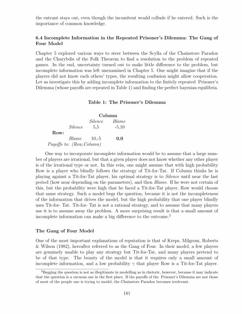
Table 1: The Prisoner’s Dilemma

ColumnSilence Blame

Silence 5,5 -5,10Row:

Blame 10,-5 0,0Payoffs to: (Row,Column)

One way to incorporate incomplete information would be to assume that a large num-ber of players are irrational, but that a given player does not know whether any other playeris of the irrational type or not. In this vein, one might assume that with high probabilityRow is a player who blindly follows the strategy of Tit-for-Tat. If Column thinks he isplaying against a Tit-for-Tat player, his optimal strategy is to Silence until near the lastperiod (how near depending on the parameters), and then Blame. If he were not certain ofthis, but the probability were high that he faced a Tit-for-Tat player, Row would choosethat same strategy. Such a model begs the question, because it is not the incompletenessof the information that drives the model, but the high probability that one player blindlyuses Tit-for- Tat. Tit-for- Tat is not a rational strategy, and to assume that many playersuse it is to assume away the problem. A more surprising result is that a small amount ofincomplete information can make a big difference to the outcome.2

The Gang of Four Model

One of the most important explanations of reputation is that of Kreps, Milgrom, Roberts& Wilson (1982), hereafter referred to as the Gang of Four. In their model, a few playersare genuinely unable to play any strategy but Tit-for-Tat, and many players pretend tobe of that type. The beauty of the model is that it requires only a small amount ofincomplete information, and a low probability γ that player Row is a Tit-for-Tat player.

2Begging the question is not as illegitimate in modelling as in rhetoric, however, because it may indicatethat the question is a vacuous one in the first place. If the payoffs of the Prisoner’s Dilemma are not thoseof most of the people one is trying to model, the Chainstore Paradox becomes irrelevant.

181

It is not unreasonable to suppose that the world contains a few mildly irrational tit-for-tatplayers, and such behavior is especially plausible among consumers, who are subject to lessevolutionary pressure than firms.

It may even be misleading to call Tit-for-Tat “irrational”, because they may just haveunusual payoffs, particularly since we will assume that they are rare. The unusual playershave a small direct influence, but they matter because other players imitate them. Even ifColumn knows that with high probability Row is just pretending to be a Tit-for-Tat player,Column does not care what the truth is so long as Row keeps on pretending. Hypocrisy isnot only the tribute vice pays to virtue; it can be just as good for deterring misbehavior.

Theorem 6.1: The Gang of Four TheoremConsider a T-stage, repeated Prisoner’s Dilemma, without discounting but with a probabilityγ of a Tit-for-Tat player. In any perfect bayesian equilibrium, the number of stages in whicheither player chooses Blame is less than some number M that depends on γ but not on T.

The significance of the Gang of Four theorem is that while the players do resort toBlame as the last period approaches, the number of periods during which they Blame isindependent of the total number of periods. Suppose M = 2, 500. If T = 2, 500, there mightbe Blame every period. But if T = 10, 000, there are 7,500 periods without a Blame move.For reasonable probabilities of the unusual type, the number of periods of cooperation canbe much larger. Wilson (unpublished) has set up an entry deterrence model in which theincumbent fights entry (the equivalent of Silence above) up to seven periods from the end,although the probability the entrant is of the unusual type is only 0.008.

The Gang of Four Theorem characterizes the equilibrium outcome rather than theequilibrium. Finding perfect bayesian equilibria is difficult and tedious, since the modellermust check all the out-of-equilibrium subgames, as well as the equilibrium path. Modellersusually content themselves with describing important characteristics of the equilibriumstrategies and payoffs.

To get a feeling for why Theorem 6.1 is correct, consider what would happen in a10,001 period game with a probability of 0.01 that Row is playing the Grim Strategy ofSilence until the first Blame, and Blame every period thereafter. Using Table 1’s payoffs,a best response for Column to a known Grim player is (Blame only in the last period,unless Row chooses Blame first, in which case respond with Blame). Both players willchoose Silence until the last period, and Column’s payoff will be 50,010 (= (10,000)(5) +10). Suppose for the moment that if Row is not Grim, he is highly aggressive, and willchoose Blame every period. If Column follows the strategy just described, the outcomewill be (Blame, Silence) in the first period and (Blame, Blame) thereafter, for a payoff toColumn of −5(= −5 + (10, 000)(0)). If the probabilities of the two outcomes are 0.01 and0.99, Column’s expected payoff from the strategy described is 495.15. If instead he followsa strategy of (Blame every period), his expected payoff is just 0.1 (= 0.01(10) + 0.99(0)).It is clearly in Column’s advantage to take a chance by cooperating with Row, even if Rowhas a 0.99 probability of following a very aggressive strategy.

The aggressive strategy, however, is not Row’s best response to Column’s strategy. Abetter response is for Row to choose Silence until the second-to- last period, and then to

182

choose Blame. Given that Column is cooperating in the early periods, Row will cooperatealso. This argument has not described what the Nash equilibrium actually is, since theiteration back and forth between Row and Column can be continued, but it does show whyColumn chooses Silence in the first period, which is the leverage the argument needs: thepayoff is so great if Row is actually the grim player that it is worthwhile for Column to riska low payoff for one period.

The Gang of Four Theorem provides a way out of the Chainstore Paradox, but itcreates a problem of multiple equilibria in much the same way as the infinitely repeatedgame. For one thing, if the asymmetry is two-sided, so both players might be unusualtypes, it becomes much less clear what happens in threat games such as Entry Deterrence.Also, what happens depends on which unusual behaviors have positive, if small, probability.Theorem 6.2 says that the modeller can make the average payoffs take any particular valuesby making the game last long enough and choosing the form of the irrationality carefully.

Theorem 6.2: The Incomplete Information Folk Theorem(Fudenberg & Maskin[1986] p. 547)For any two-person repeated game without discounting, the modeller can choose a form ofirrationality so that for any probability ε > 0 there is some finite number of repetitions suchthat with probability (1− ε) a player is rational and the average payoffs in some sequentialequilibrium are closer than ε to any desired payoffs greater than the minimax payoffs.

6.5 The Axelrod Tournament

Another way to approach the repeated Prisoner’s Dilemma is through experiments, suchas the round robin tournament described by political scientist Robert Axelrod in his 1984book. Contestants submitted strategies for a 200-repetition Prisoner’s Dilemma . Sincethe strategies could not be updated during play, players could precommit, but the strategiescould be as complicated as they wished. If a player wanted to specify a strategy whichsimulated subgame perfectness by adapting to past history just as a noncommitted playerwould, he was free to do so, but he could also submit a non-perfect strategy such as Tit-for-Tat or the slightly more forgiving Tit-for-Two-Tats. Strategies were submitted in the formof computer programs that were matched with each other and played automatically. InAxelrod’s first tournament, 14 programs were submitted as entries. Every program playedevery other program, and the winner was the one with the greatest sum of payoffs over allthe plays. The winner was Anatol Rapoport, whose strategy was Tit-for-Tat.

The tournament helps to show which strategies are robust against a variety of otherstrategies in a game with given parameters. It is quite different from trying to find aNash equilibrium, because it is not common knowledge what the equilibrium is in such atournament. The situation could be viewed as a game of incomplete information in whichNature chooses the number and cognitive abilities of the players and their priors regardingeach other.

183

After the results of the first tournament were announced, Axelrod ran a second tourna-ment, adding a probability θ = 0.00346 that the game would end each round so as to avoidthe Chainstore Paradox. The winner among the 62 entrants was again Anatol Rapoport,and again he used Tit-for-Tat.

Before choosing his tournament strategy, Rapoport had written an entire book onThe Prisoner’s Dilemma in analysis, experiment, and simulation (Rapoport & Chammah[1965]). Why did he choose such a simple strategy as Tit-for-Tat? Axelrod points out thatTit-for-Tat has three strong points.

1. It never initiates blaming (niceness);

2. It retaliates instantly against blaming (provocability);

3. It forgives someone who plays Blame but then goes back to cooperating (it is for-giving).

Despite these advantages, care must be taken in interpreting the results of the tourna-ment. It does not follow that Tit-for-Tat is the best strategy, or that cooperative behaviorshould always be expected in repeated games.

First, Tit-for-Tat never beats any other strategy in a one-on-one contest. It won thetournament by piling up points through cooperation, having lots of high score plays andvery few low score plays. In an elimination tournament, Tit-for- Tat would be eliminatedvery early, because it scores high payoffs but never the highest payoff.

Second, the other players’ strategies matter to the success of Tit-for-Tat. In neithertournament were the strategies submitted a Nash equilibrium. If a player knew what strate-gies he was facing, he would want to revise his own. Some of the strategies submitted in thesecond tournament would have won the first, but they did poorly because the environmenthad changed. Other programs, designed to try to probe the strategies of their opposition,wasted too many (Blame, Blame) episodes on the learning process, but if the games hadlasted a thousand repetitions they would have done better.

Third, in a game in which players occasionally blamed because of trembles, two Tit-for-Tat players facing each other would do very badly. The strategy instantly punishes ablaming player, and it has no provision for ending the punishment phase.

Optimality depends on the environment. When information is complete and the payoffsare all common knowledge, blaming is the only equilibrium outcome. In practically anyreal-world setting, however, information is slightly incomplete, so cooperation becomesmore plausible. Tit-for-Tat is suboptimal for any given environment, but it is robust acrossenvironments, and that is its advantage.

184

6.6 Credit and the Age of the Firm: The Diamond Model

An example of another way to look at reputation is Diamond’s model of credit terms, whichseeks to explain why older firms get cheaper credit using a game similar to the Gang of Fourmodel. Telser (1966) suggested that predatory pricing would be a credible threat if theincumbent had access to cheaper credit than the entrant, and so could hold out for moreperiods of losses before going bankrupt. While one might wonder whether this is effectiveprotection against entry— what if the entrant is a large old firm from another industry?—we shall focus on how better-established firms might get cheaper credit.

D. Diamond (1989) aims to explain why old firms are less likely than young firms todefault on debt. His model has both adverse selection, because firms differ in type, andmoral hazard, because they take hidden actions. The three types of firms, R, S, and RS,are “born” at time zero and borrow to finance projects at the start of each of T periods. Wemust imagine that there are overlapping generations of firms, so that at any point in timea variety of ages are coexisting, but the model looks at the lifecycle of only one generation.All the players are risk neutral. Type RS firms can choose independently risky projects withnegative expected values or safe projects with low but positive expected values. Althoughthe risky projects are worse in expectation, if they are successful the return is much higherthan from safe projects. Type R firms can only choose risky projects, and type S firms onlysafe projects. At the end of each period the projects bring in their profits and loans arerepaid, after which new loans and projects are chosen for the next period. Lenders cannottell which project is chosen or what a firm’s current profits are, but they can seize thefirm’s assets if a loan is not repaid, which always happens if the risky project was chosenand turned out unsuccessfully.

This game foreshadows two other models of credit that will be described in this book,the Repossession Game of section 8.4 and the Stiglitz-Weiss model of section 9.6. Both willbe one-shot games in which the bank worried about not being repaid; in the RepossessionGame because the borrower did not exert enough effort, and in the Stiglitz-Weiss modelbecause he was of an undesirable type that could not repay. The Diamond model is amixture of adverse selection and moral hazard: the borrowers differ in type, but someborrowers have a choice of action.

The equilibrium path has three parts. The RS firms start by choosing risky projects.Their downside risk is limited by bankruptcy, but if the project is successful the firm keepslarge residual profits after repaying the loan. Over time, the number of firms with accessto the risky project (the RS’s and R’s) diminishes through bankruptcy, while the numberof S’s remains unchanged. Lenders can therefore maintain zero profits while loweringtheir interest rates. When the interest rate falls, the value of a stream of safe investmentprofits minus interest payments rises relative to the expected value of the few periods ofrisky returns minus interest payments before bankruptcy. After the interest rate has fallenenough, the second phase of the game begins when the RS firms switch to safe projects ata period we will call t1. Only the tiny and diminishing group of type R firms continue tochoose risky projects. Since the lenders know that the RS firms switch, the interest ratecan fall sharply at t1. A firm that is older is less likely to be a type R, so it is charged alower interest rate. Figure 4 shows the path of the interest rate over time.

185

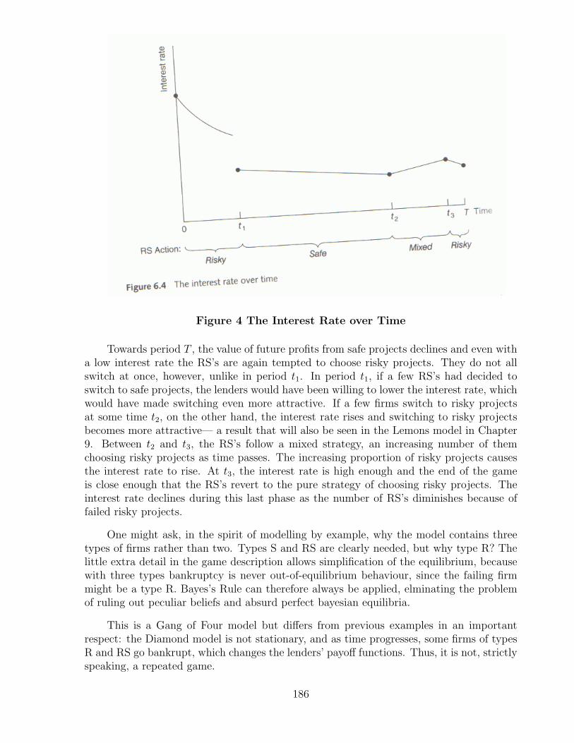
Figure 4 The Interest Rate over Time

Towards period T , the value of future profits from safe projects declines and even witha low interest rate the RS’s are again tempted to choose risky projects. They do not allswitch at once, however, unlike in period t1. In period t1, if a few RS’s had decided toswitch to safe projects, the lenders would have been willing to lower the interest rate, whichwould have made switching even more attractive. If a few firms switch to risky projectsat some time t2, on the other hand, the interest rate rises and switching to risky projectsbecomes more attractive— a result that will also be seen in the Lemons model in Chapter9. Between t2 and t3, the RS’s follow a mixed strategy, an increasing number of themchoosing risky projects as time passes. The increasing proportion of risky projects causesthe interest rate to rise. At t3, the interest rate is high enough and the end of the gameis close enough that the RS’s revert to the pure strategy of choosing risky projects. Theinterest rate declines during this last phase as the number of RS’s diminishes because offailed risky projects.

One might ask, in the spirit of modelling by example, why the model contains threetypes of firms rather than two. Types S and RS are clearly needed, but why type R? Thelittle extra detail in the game description allows simplification of the equilibrium, becausewith three types bankruptcy is never out-of-equilibrium behaviour, since the failing firmmight be a type R. Bayes’s Rule can therefore always be applied, elminating the problemof ruling out peculiar beliefs and absurd perfect bayesian equilibria.

This is a Gang of Four model but differs from previous examples in an importantrespect: the Diamond model is not stationary, and as time progresses, some firms of typesR and RS go bankrupt, which changes the lenders’ payoff functions. Thus, it is not, strictlyspeaking, a repeated game.

186

Notes

N6.1 Perfect Bayesian Equilibrium: Entry Deterrence I and II

• Section 4.1 showed that even in games of perfect information, not every subgame perfectequilibrium is trembling-hand perfect. In games of perfect information, however, everysubgame perfect equilibrium is a perfect bayesian equilibrium, since no out-of-equilibriumbeliefs need to be specified.

N6.2 Refining Perfect Bayesian Equilibrium: The PhD Admissions Game

• Fudenberg & Tirole (1991b) is a careful analysis of the issues involved in defining perfectbayesian equilibrium.

• Section 6.2 is about debatable ways of restricting beliefs such as passive conjectures orequilibrium dominance, but less controversial restrictions are sometimes useful. In a three-player game, consider what happens when Smith and Jones have incomplete informationabout Brown, and then Jones deviates. If it was Brown himself who had deviated, onemight think that the other players might deduce something about Brown’s type. Butshould they update their priors on Brown because Jones has deviated? Especially, shouldJones updated his beliefs, just because he himself deviated? Passive conjectures seems muchmore reasonable.

If, to take a second possibility, Brown himself does deviate, is it reasonable for the out-of-equilibrium beliefs to specify that Smith and Jones update their beliefs about Brown indifferent ways? This seems dubious in light of the Harsanyi doctrine that everyone beginswith the same priors.

On the other hand, consider a tremble interpretation of out-of- equilibrium moves. Maybe ifJones trembles and picks the wrong strategy, that really does say something about Brown’stype. Jones might tremble more often, for example, if Brown’s type is strong than if itis weak. Jones himself might learn from his own trembles. Once we are in the realm ofnon-bayesian beliefs, it is hard to know what to do without a real-world context.

Dominance and tremble arguments used to rule out Nash equilibria apply to past, present(in simultaneous move games), and future actions of the other player. Belief arguments onlydepend on past actions, because they rely on the uninformed player observing behavior andinterpreting it. Thus, for example, a tremble or weak dominance argument might say aplayer should take action 1 instead of 2 because although their payoffs are equal, action 2would lead to a very low payoff if the other player later trembled and chose an unintendedaction that hurt both of them. An argument based on beliefs would not work in such agame.

• For discussions of the appropriateness of different equilibrium concepts in actual economicmodels see Rubinstein (1985b) on bargaining, Shleifer & Vishny (1986) on greenmail andD. Hirshleifer & Titman (1990) on tender offers.

• Exotic refinements. Binmore (1990) and Kreps (1990b) are booklength treatments ofrationality and equilibrium concepts. Van Damme (1989) introduces the curious “moneyburning” idea of “forward induction.”

• The Beer-Quiche Game of Cho & Kreps (1987). To illustrate their “intuitive criterion”,Cho and Kreps use the Beer-Quiche Game. In this game, Player I might be either weak or

187

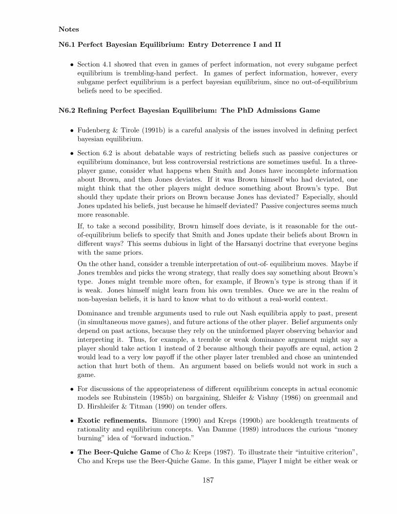
strong in his duelling ability, but he wishes to avoid a duel even if he thinks he can win.Player II wishes to fight a duel only if player I is weak, which has a probability of 0.1.Player II does not know player I’s type, but he observes what player I has for breakfast. Heknows that weak players prefer quiche for breakast, while strong players prefer beer. Thepayoffs are shown in Figure 5.

Figure 5 illustrates a few twists on how to draw an extensive form. It begins with Nature’schoice of Strong or Weak in the middle of the diagram. Player I then chooses whether tobreakfast on beer or quiche. Player II’s nodes are connected by a dotted line if they are inthe same information set. Player II chooses Duel or Don′t, and payoffs are then received.

Figure 5 The Beer-Quiche Game

This game has two perfect bayesian equilibrium outcomes, both of which are pooling. InE1, player I has beer for breakfast regardless of type, and Player II chooses not to duel.This is supported by the out-of-equilibrium belief that a quiche-eating player I is weak withprobability over 0.5, in which case player II would choose to duel on observing quiche. InE2, player I has quiche for breakfast regardless of type, and player II chooses not to duel.This is supported by the out-of-equilibrium belief that a beer-drinking player I is weak withprobability greater than 0.5, in which case player II would choose to duel on observing beer.

Passive conjectures and the intuitive criterion both rule out equilibrium E2. According tothe reasoning of the intuitive criterion, player I could deviate without fear of a duel bygiving the following convincing speech,

I am having beer for breakfast, which ought to convince you I am strong.The only conceivable benefit to me of breakfasting on beer comes if I am strong.I would never wish to have beer for breakfast if I were weak, but if I am strongand this message is convincing, then I benefit from having beer for breakfast.

N6.5 The Axelrod tournament

188

• Hofstadter (1983) is a nice discussion of the Prisoner’s Dilemma and the Axelrod tour-nament by an intelligent computer scientist who came to the subject untouched by thepreconceptions or training of economics. It is useful for elementary economics classes. Ax-elrod’s 1984 book provides a fuller treatment.

189

Problems

6.1. Cournot Duopoly under Incomplete Information about Costs (hard)This problem introduces incomplete information into the Cournot model of Chapter 3 and allowsfor a continuum of player types.

(a) Modify the Cournot Game of Chapter 3 by specifying that Apex’s average cost of productionbe c per unit, while Brydox’s remains zero. What are the outputs of each firm if the costsare common knowledge? What are the numerical values if c = 10?

(b) Let Apex’s cost c be cmax with probability θ and 0 with probability 1 − θ, so Apex is oneof two types. Brydox does not know Apex’s type. What are the outputs of each firm?

(c) Let Apex’s cost c be drawn from the interval [0, cmax] using the uniform distribution, sothere is a continuum of types. Brydox does not know Apex’s type. What are the outputsof each firm?

(d) Outputs were 40 for each firm in the zero-cost game in chapter 3. Check your answers inparts (b) and (c) by seeing what happens if cmax = 0.

(e) Let cmax = 20 and θ = 0.5, so the expectation of Apex’s average cost is 10 in parts (a), (b),and (c). What are the average outputs for Apex in each case?

(f) Modify the model of part (b) so that cmax = 20 and θ = 0.5, but somehow c = 30. Whatoutputs do your formulas from part (b) generate? Is there anything this could sensiblymodel?

Problem 6.2. Limit Pricing (medium) (see Milgrom and Roberts [1982a])An incumbent firm operates in the local computer market, which is a natural monopoly in whichonly one firm can survive. The incumbent knows his own operating cost c, which is 20 withprobability 0.2 and 30 with probability 0.8.

In the first period, the incumbent can price Low, losing 40 in profits, or High, losing nothingif his cost is c = 20. If his cost is c = 30, however, then pricing Low he loses 180 in profits. (Youmight imagine that all consumers have a reservation price that is High, so a static monopolistwould choose that price whether marginal cost was 20 or 30.)

A potential entrant knows those probabilities, but not the incumbent’s exact cost. In thesecond period, the entrant can enter at a cost of 70, and his operating cost of 25 is commonknowledge. If there are two firms in the market, each incurs an immediate loss of 50, but onethen drops out and the survivor earns the monopoly revenue of 200 and pays his operating cost.There is no discounting: r = 0.

(a) In a perfect bayesian equilibrium in which the incumbent prices High regardless of its costs(a pooling equilibrium), about what do out-of- equilibrium beliefs have to be specified?

(b) Find a pooling perfect bayesian equilibrium, in which the incumbent always chooses thesame price no matter what his costs may be.

(c) What is a set of out-of-equilibrium beliefs that do not support a pooling equilibrium at aHigh price?

190

(d) What is a separating equilibrium for this game?

6.3. Symmetric Information and Prior Beliefs (medium)In the Expensive-Talk Game of Table 2, the Battle of the Sexes is preceded by by a communicationmove in which the man chooses Silence or Talk. Talk costs 1 payoff unit, and consists of adeclaration by the man that he is going to the prize fight. This declaration is just talk; it is notbinding on him.

Table 2: Subgame Payoffs in the Expensive-Talk Game

WomanFight Ballet

F ight 3,1 0, 0Man:

Ballet 0, 0 1,3Payoffs to: (Man, Woman)

(a) Draw the extensive form for this game, putting the man’s move first in the simultaneous-move subgame.

(b) What are the strategy sets for the game? (Start with the woman’s.)

(c) What are the three perfect pure-strategy equilibrium outcomes in terms of observed actions?(Remember: strategies are not the same thing as outcomes.)

(d) Describe the equilibrium strategies for a perfect equilibrium in which the man chooses totalk.

(e) The idea of “forward induction” says that an equilibrium should remain an equilibrium evenif strategies dominated in that equilibrium are removed from the game and the procedureis iterated. Show that this procedure rules out SBB as an equilibrium outcome.(See VanDamme [1989]. In fact, this procedure rules out TFF (Talk, Fight, Fight) also.)

6.4. Lack of Common Knowledge (medium)This problem looks at what happens if the parameter values in Entry Deterrence V are changed.

(a) Why does Pr(Strong|Enter, Nature said nothing) = 0.95 not support the equilibrium inSection 6.3?

(b) Why is the equilibrium in Section 6.3 not an equilibrium if 0.7 is the probability that Naturetells the incumbent?

(c) Describe the equilibrium if 0.7 is the probability that Nature tells the incumbent. For whatout-of-equilibrium beliefs does this remain the equilibrium?

191

The Repeated Prisoner’s Dilemma under Incomplete Information: A ClassroomGame for Chapter 6

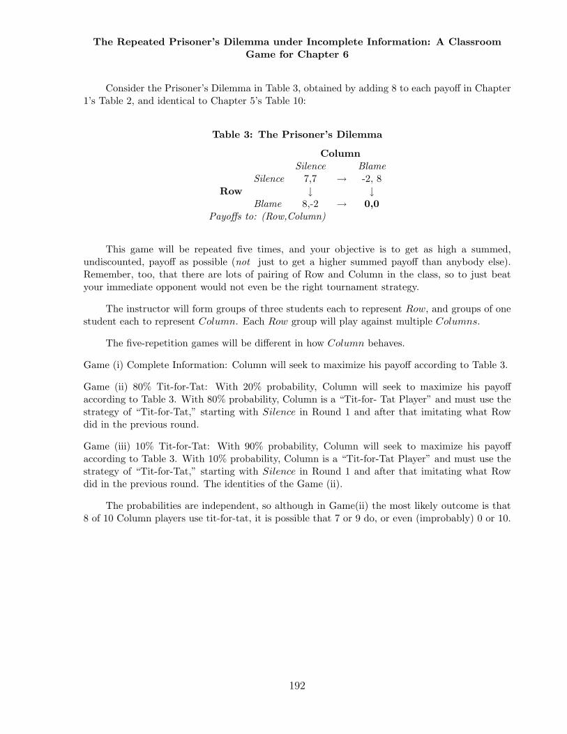
Consider the Prisoner’s Dilemma in Table 3, obtained by adding 8 to each payoff in Chapter1’s Table 2, and identical to Chapter 5’s Table 10:

Table 3: The Prisoner’s Dilemma

ColumnSilence Blame

Silence 7,7 → -2, 8Row ↓ ↓

Blame 8,-2 → 0,0Payoffs to: (Row,Column)

This game will be repeated five times, and your objective is to get as high a summed,undiscounted, payoff as possible (not just to get a higher summed payoff than anybody else).Remember, too, that there are lots of pairing of Row and Column in the class, so to just beatyour immediate opponent would not even be the right tournament strategy.

The instructor will form groups of three students each to represent Row, and groups of onestudent each to represent Column. Each Row group will play against multiple Columns.

The five-repetition games will be different in how Column behaves.

Game (i) Complete Information: Column will seek to maximize his payoff according to Table 3.

Game (ii) 80% Tit-for-Tat: With 20% probability, Column will seek to maximize his payoffaccording to Table 3. With 80% probability, Column is a “Tit-for- Tat Player” and must use thestrategy of “Tit-for-Tat,” starting with Silence in Round 1 and after that imitating what Rowdid in the previous round.

Game (iii) 10% Tit-for-Tat: With 90% probability, Column will seek to maximize his payoffaccording to Table 3. With 10% probability, Column is a “Tit-for-Tat Player” and must use thestrategy of “Tit-for-Tat,” starting with Silence in Round 1 and after that imitating what Rowdid in the previous round. The identities of the Game (ii).

The probabilities are independent, so although in Game(ii) the most likely outcome is that8 of 10 Column players use tit-for-tat, it is possible that 7 or 9 do, or even (improbably) 0 or 10.

192