6 Image Processing: Continuous Imagespeople.csail.mit.edu/bkph/courses/papers/RoVis/ch6_FT_continuous.… · 6 Image Processing: Continuous Images It is often useful to transform

6

Image Processing:Continuous Images

It is often useful to transform an image in some way, producing a new onethat is more amenable to further manipulation. Image processing involvesthe search for methods to accomplish such transformations. Most of themethods examined so far are linear and shift-invariant. Methods withthese properties allow us to apply powerful analytic tools. We show inthis chapter that linear, shift-invariant systems can be characterized byconvolution, an operation introduced in its one-dimensional form when wediscussed the probability distribution of the sum of two random variables.

We also demonstrate the utility of the concept of spatial frequency andof transformations between the spatial and the frequency domains. Image-processing systems, whether optical or digital, can be characterized eitherin the spatial domain, by their point-spread function, or in the frequencydomain, by their modulation-transfer function. The tools discussed in thischapter will be applied to the analysis of partial differential operators usedin edge detection, and to the analysis of optimal filtering methods for thesuppression of noise.

Most of the methods discussed here are simple extensions to two di-mensions of linear systems techniques for one-dimensional signals, but weshall not assume that the reader is familiar with these techniques. We treatthe continuous case in this chapter and the discrete case in the next.

104 Image Processing: Continuous Images

6.1 Linear, Shift-Invariant Systems

An image can be thought of as a two-dimensional signal. We can developan approach to image processing based on this observation. Consider anout-of-focus imaging system (figure 6-1). We can think of the image g(x, y)produced by the defocused system as a processed version of the ideal im-age, f(x, y), that one would obtain in a correctly focused imaging system.Now, if the lighting is changed so as to double the brightness of the idealimage, the brightness of the out-of-focus image is also doubled. Further,if the imaging system is moved slightly, so that the ideal image is shiftedin the image plane, the out-of-focus image is similarly shifted. The trans-formation from the ideal image to that in the out-of-focus system is saidto be a linear, shift-invariant operation. In fact, incoherent optical image-processing systems that are more complicated are typically also linear andshift-invariant. These terms will now be defined more precisely.

Consider a two-dimensional system that produces outputs g1(x, y) andg2(x, y) when given inputs f1(x, y) and f2(x, y), respectively:

f1 → → g1

f2 → → g2

6.1 Linear, Shift-Invariant Systems 105

The system is called linear if the output αg1(x, y) + βg2(x, y) is producedwhen the input is αf1(x, y) + βf2(x, y), for arbitrary α and β:

α f1 + β f2 → → α g1 + β g2

Most real systems are limited in their maximum response and thus cannotbe strictly linear. Moreover, brightness, which is power per unit area,cannot be negative. The original input, an image, is thus restricted tononnegative values. Intermediate results of our computations can, however,have arbitrary values.

Now consider a system that produces output g(x, y) when given inputf(x, y):

f(x, y) → → g(x, y)

The system is called shift-invariant if it produces the shifted output g(x −a, y − b) when given the shifted input f(x − a, y − b), for arbitrary a and b:

f(x − a, y − b) → → g(x − a, y − b)

In practice, images are limited in area, so that shift invariance only holds forlimited displacements. Moreover, aberrations in optical imaging systemsvary with the distance from the optical axis; such systems are thereforeonly approximately shift-invariant.

Methods for analyzing linear, shift-invariant systems are important forunderstanding the properties of image-forming systems. System shortcom-ings can often be discussed in terms of the linear, shift-invariant systemthat would transform the ideal image into the one actually observed. Moreimportantly for us, a study of linear, shift-invariant systems leads to usefulalgorithms for processing images using either optical or digital methods.

A simple example of a linear, shift-invariant system is one that producesthe derivative of its input with respect to x or y. Linearity follows fromthe rules for differentiating the product of a constant and some functionand the rule for differentiating the sum of two functions. Shift invarianceis equally easy to prove. Systems taking derivatives will prove useful aspreprocessing stages in edge-detection systems.

We start by considering continuous images in order to lay the ground-work for the discrete operations. Linear, shift-invariant systems for pro-cessing images are extensions to two dimensions of one-dimensional linear,


shift-invariant systems, such as simple passive electrical circuits. Not sur-prisingly, most of the results presented here can be derived using simpleextensions of methods used to prove similar results applying to the one-dimensional case. To simplify matters, we shall factor functions of twovariables into products of two functions of one variable whenever possi-ble. This will allow us to split the two-dimensional integrals that arise intoproducts of one-dimensional integrals.

In the analysis of one-dimensional systems, functions of time are typi-cally used as both inputs and outputs. No system can anticipate its input.This places a severe restriction on systems for processing one-dimensionalsignals: They have to be causal. Only those that obey this restrictioncan be physically realized. There is no such problem in the synthesis oftwo-dimensional systems.

While we inherit the powerful methods of signal processing from one-dimensional systems, we must also point out the shortcomings. The con-straints of linearity and shift invariance are severe and greatly limit thekinds of things we can do with an image. Still, it is hard to make progresswithout some guiding theory.

6.2 Convolution and the Point-Spread Function

Consider a system that, given an input f(x, y), produces as its output

g(x, y) =∫ ∞

−∞

∫ ∞

−∞f(x − ξ, y − η)h(ξ, η) dξ dη.

Here g is said to be the convolution of f and h. It is easy to show that sucha system is linear by applying it to αf1(x, y)+βf2(x, y) and noting that theoutput is αg1(x, y) + βg2(x, y). Here again g1(x, y) is the output producedwhen f1(x, y) is the input and g2(x, y) is the output produced when f2(x, y)is the input. The result follows from the rule for integrating the productof a constant and a function and from the rule for integrating the sum oftwo functions. It is also easy to show that the system is shift-invariant byapplying it to f(x − a, y − b) and noting that the output is g(x − a, y − b).Thus a system whose response can be described by a convolution is linearand shift-invariant. We shall soon show the converse:

• Any linear, shift-invariant system performs a convolution.

Convolution is usually denoted by the symbol ⊗. So the above formula canbe abbreviated

g = f ⊗ h.

6.2 Convolution and the Point-Spread Function 107

It would be useful to relate the function h(x, y) to some observableproperty of the system. Given an arbitrary function h(x, y), can we alwaysfind an input f(x, y) that causes the system to produce h(x, y) as output?That is, can we find an f(x, y) such that

h(x, y) =∫ ∞

−∞

∫ ∞

−∞f(x − ξ, y − η)h(ξ, η) dξ dη ?

Cursory inspection suggests that if this is to be true for arbitrary h(x, y),then f(x, y) needs to be zero at all points away from the origin and “in-finite” at the origin. The “function” we are looking for is called the unitimpulse, denoted δ(x, y). It is also sometimes referred to as the Dirac deltafunction.

Loosely speaking, δ(x, y) is zero everywhere except at the origin, whereit is “infinite.” The integral of δ(x, y) over any region including the originis one. (If we think of a function of x and y as a surface, then this integralis the volume under that surface.) The impulse δ(x, y) is not a functionin the classical sense (that is, it is not defined by giving its value for allarguments). It is a generalized function that can be thought of as the“limit” as ε → 0 of a series of square pulses of width 2ε in x and y and ofheight 1/(4ε2). We shall have more to say about this later, but for now wesimply note the sifting property,∫ ∞

−∞

∫ ∞

−∞δ(x, y)h(x, y) dx dy = h(0, 0),

by which the impulse can be defined. It follows that∫ ∞

−∞

∫ ∞

−∞δ(x − ξ, y − η)h(ξ, η) dξ dη = h(x, y),

as can be seen by a simple change of variables. By comparing this with ouroriginal equation for the output of the system, we see that h(x, y) is theresponse of the system when presented with the unit impulse as input.

Considered as an image, δ(x, y) is black everywhere except at the origin,where there is a point of bright light. Thus h(x, y) tells us how the systemblurs or spreads out a point of light. In the case of a two-dimensionalsystem it is called the point-spread function. It is the response of the two-dimensional system to an impulse and is thus analogous to the familiarimpulse response of a one-dimensional system.

We now want to show that the output of any linear, shift-invariantsystem is related to its input by convolution. The point-spread function of


the system, h(x, y), can be determined by applying the test input δ(x, y).Given that the response to an impulse is now known, it is convenient tothink of the input, f(x, y), as made up of an infinite collection of shifted,scaled impulses,

k(ξ, η)δ(x − ξ, y − η).

A simple geometric construction will help show how this can be done.Divide the xy-plane into squares of width ε. On each such elementarysquare erect a pulse of height equal to the average of f(x, y) in the square.Figure 6-2 shows a cross section through such a two-dimensional arrayof square pulses. The function f(x, y) is approximated by the piecewise-constant function that is the sum of all these pulses.

We can go one step further and replace each rectangular pulse by animpulse at the center of its square base. The volume under the impulse canbe made equal to the volume of the rectangular pulse, that is, the integralof the function f(x, y) over the elementary square. If the function f(x, y)is continuous, and ε is small enough, one can approximate this integral bythe product of the value of f(x, y) at the center of the square and the areaof the square. The desired result is obtained in the limit as we let ε → 0.

The same decomposition of f(x, y) in terms of impulses can be obtainedby appealing to the sifting property of the unit impulse function. Either

6.2 Convolution and the Point-Spread Function 109

way, we find that

f(x, y) =∫ ∞

−∞

∫ ∞

−∞f(ξ, η) δ(x − ξ, y − η) dξ dη.


Having decomposed the function in terms of impulses, we can determine theoverall output, g(x, y), when f(x, y) is the input, by adding the responsesof the system to the shifted, scaled impulses. This is so because the systemis linear.

The response to k δ(x − ξ, y − η) is k h(x − ξ, y − η), since the systemis shift-invariant. Thus, since k is just f(ξ, η),

g(x, y) =∫ ∞

−∞

∫ ∞

−∞f(ξ, η) h(x − ξ, y − η) dξ dη.

This can be written in the form h ⊗ f . We show below that convolution iscommutative, so that h ⊗ f = f ⊗ h, and so

g(x, y) =∫ ∞

−∞

∫ ∞

−∞f(x − ξ, y − η) h(ξ, η) dξ dη.

Linear, shift-invariant systems can always be described by a suitable point-spread function h(x, y). Using this function we can compute the outputg(x, y), given an arbitrary input f(x, y). The point-spread function is acomplete characterization of a linear, shift-invariant system. We have thusshown that a linear, shift-invariant system performs a convolution.

We now show that convolution is commutative, that is, that

b ⊗ a = a ⊗ b.

Let c = a ⊗ b, or

c(x, y) =∫ ∞

−∞

∫ ∞

−∞a(x − ξ, y − η) b(ξ, η) dξ dη.

Now let x − ξ = α and y − η = β, so that

c(x, y) =∫ ∞

−∞

∫ ∞

−∞a(α, β) b(x − α, y − β) dα dβ.

Since α and β are arbitrary dummy variables, we can substitute ξ and η

for them without changing the value of the integral. We obtain

c(x, y) =∫ ∞

−∞

∫ ∞

−∞b(x − ξ, y − η) a(ξ, η) dξ dη,

which is b ⊗ a. Convolution is also associative; that is,

(a ⊗ b) ⊗ c = a ⊗ (b ⊗ c).

6.3 The Modulation-Transfer Function 111

This allows us to consider the cascade of two systems with point-spreadfunctions h1(x, y) and h2(x, y):

f → h1 h2 → g

If the input is f(x, y), then the output of the first system is f⊗h1. This newsignal is the input of the second system, and so the output of the secondsystem is (f ⊗ h1) ⊗ h2. This can be written in the form f ⊗ (h1 ⊗ h2),that is, the output produced when the input f is applied to a system withpoint-spread function h1 ⊗ h2:

f → h1 ⊗ h2 → g

6.3 The Modulation-Transfer Function

It is harder to visualize the effect of convolution than it is the multiplica-tion of two functions. Because convolution in the spatial domain becomesmultiplication in the frequency domain, a transformation to the frequencydomain is attractive in the case of linear, shift-invariant systems. Beforewe can explore these ideas, however, we must understand what frequencymeans for two-dimensional systems.

In the case of one-dimensional linear, shift-invariant systems we findthat eiωt is an eigenfunction of convolution. An eigenfunction of a systemis a function that is reproduced with at most a change in amplitude:

eiωt → → A(ω) eiωt

Here A(ω) is the (possibly complex) factor by which the input signal ismultiplied. That is, if we apply a complex exponential to a linear, shift-invariant system, we obtain a similar complex exponential waveform at theoutput, just scaled and shifted in phase. We call ω the frequency of theeigenfunction. In practice, we use real waveforms like cos ωt and sinωt,corresponding to the real and imaginary parts of eiωt. The relationshipbetween the two forms is, of course, just

eiwt = cos ωt + i sin ωt.

The complex exponential form is used in deriving results because it makesthe expressions more compact and helps avoid the need to treat cosinesand sines separately.


In a two-dimensional linear, shift-invariant system, the input f(x, y) =e+i(ux+vy) gives rise to the output

g(x, y) =∫ ∞

−∞

∫ ∞

−∞ei(u(x−ξ)+v(y−η))h(ξ, η) dξ dη,

or

g(x, y) = e+i(ux+vy)∫ ∞

−∞

∫ ∞

−∞e−i(uξ+vη)h(ξ, η) dξ dη.

The double integral on the right is a function of u and v only, and theoutput g(x, y) is therefore just a scaled, possibly shifted, version of theinput f(x, y). Thus e+i(ux+vy) is an eigenfunction of convolution in twodimensions:

ei(ux+vy) → → A(u, v) ei(ux+vy)

Note that frequency now has two components, u and v. We refer to theuv-plane as the frequency domain, in contrast to the xy-plane, which isreferred to as the spatial domain.

The real waveforms cos(ux+vy) and sin(ux+vy) correspond to wavesin two dimensions. The maxima and minima of cos(ux+ vy) lie on parallelequidistant ridges along the lines

ux + vy = kπ

for integer k (figure 6-3). Taking a cut through the surface at right anglesto these lines, that is, in the direction (u, v), gives us sinusoidal waves withwavelength

λ =2π√

u2 + v2.

Such waves cannot occur on their own in an imaging system since brightness

6.3 The Modulation-Transfer Function 113

cannot be negative. There must be an added constant offset.


6.4 Fourier Transform and Filtering 115

If we let

H(u, v) =∫ ∞

−∞

∫ ∞

−∞e−i(uξ+vη)h(ξ, η) dξ dη,

then, in the special case treated so far,

g(x, y) = H(u, v) f(x, y),

as can be seen from the integral given previously. Thus H(u, v) character-izes the system for sinusoidal waveforms, just as h(x, y) does for impulsivewaveforms. For each frequency, it tells us the response of the system inamplitude and phase. In the case of a two-dimensional system it is calledthe modulation-transfer function. It is the frequency response of the two-dimensional system and so is analogous to the familiar frequency responseof a one-dimensional system. (Note that H(u, v) need not be real-valued.)

Just as we can learn much about the quality of an audio amplifierfrom its frequency response curve, so we can compare camera lenses, forexample, by looking at their modulation-transfer function plots.

6.4 Fourier Transform and Filtering

An input f(x, y) can be considered to be the sum of an infinite numberof sinusoidal waves, just as earlier we thought of it as the sum of an infi-nite number of impulses. This is another convenient way to decompose theinput, since we once again already know the system’s response to each com-ponent, provided we are given the modulation-transfer function H(u, v). Ifwe decompose f(x, y) as

f(x, y) =1

4π2

∫ ∞

−∞

∫ ∞

−∞F (u, v)e+i(ux+vy) du dv,

then

g(x, y) =1

4π2

∫ ∞

−∞

∫ ∞

−∞H(u, v) F (u, v)e+i(ux+vy) du dv.

(The 1/4π2 occurs here for consistency with formulae introduced later on.)The only problem is that the decomposition into sinusoidal waves is notquite as trivial as the decomposition into impulses. How do we find F (u, v)given f(x, y)? As we shall demonstrate in a moment, the answer turns outto be

F (u, v) =∫ ∞

−∞

∫ ∞

−∞f(x, y)e−i(ux+vy) dx dy


provided that this integral exists. We can see that this might be so bychanging variables,

F (u, v) =∫ ∞

−∞

∫ ∞

−∞f(α, β)e−i(uα+vβ) dα dβ,

and substituting into the expression for f(x, y) to obtain

14π2

∫ ∞

−∞

∫ ∞

−∞f(α, β)

[∫ ∞

−∞

∫ ∞

−∞ei(u(x−α)+v(y−β)) du dv

]dα dβ.

The inner integral does not converge. We show later, using so-called con-vergence factors, that it can be considered to equal 4π2δ(x−α, y −β). Wetherefore have∫ ∞

−∞

∫ ∞

−∞f(α, β)δ(x − α, y − β) dα dβ = f(x, y),

so that

14π2

∫ ∞

−∞

∫ ∞

−∞F (u, v)e+i(ux+vy) du dv = f(x, y).

F (u, v) is called the Fourier transform of f(x, y). Similarly, we can definethe Fourier transform G(u, v) of the output g(x, y). Finally,

G(u, v) = H(u, v) F (u, v),

which is simpler than

g(x, y) =∫ ∞

−∞

∫ ∞

−∞f(x − ξ, y − η)h(ξ, η) dξ dη.

Thus convolution has been transformed into multiplication!We also see once again that the modulation-transfer function H(u, v)

specifies how the system attenuates or amplifies each component F (u, v)of the input. A linear, shift-invariant system thus acts as a filter that se-lectively attenuates or amplifies various parts of the spectrum of possiblefrequencies. It can also shift their phase, but this is all it does. We mightconclude that restricting ourselves to linear, shift-invariant systems seri-ously limits what we can accomplish, but at the same time it allows us toderive a lot of useful results, because the mathematics is manageable.

Note the minor asymmetry in the expressions for the forward Fouriertransform

F (u, v) =∫ ∞

−∞

∫ ∞

−∞f(x, y)e−i(ux+vy) dx dy

6.5 The Fourier Transform of Convolution 117

and the inverse transform

f(x, y) =1

4π2

∫ ∞

−∞

∫ ∞

−∞F (u, v)e+i(ux+vy) du dv.

The constant multipliers are split up in this way to be consistent withother textbooks. The fact that the transforms are almost symmetric makesit possible to deduce properties that apply to the inverse transform, givenproperties that apply to the forward transform. Observe, however, thatF (u, v) is generally complex, whereas f(x, y) is always real. Note also thatH(u, v) is the Fourier transform of h(x, y).

Not all functions have a Fourier transform. Functions in certain simpleclasses are equal to the Fourier integrals of their Fourier transforms. But itis hard to characterize exactly which functions do, and which do not, havea transform.

A different kind of difficulty is that the integrals are taken over thewhole xy-plane, whereas imaging devices only produce usable images overa finite part of the image plane. Moreover, computers only use discretesamples of these images. These two issues will be discussed in more detailin the next chapter.

6.5 The Fourier Transform of Convolution

Let c = a ⊗ b; then the Fourier transform C(u, v) of c(x, y) is∫ ∞

−∞

∫ ∞

−∞

[∫ ∞

−∞

∫ ∞

−∞a(x − ξ, y − η)b(ξ, η) dξ dη

]e−i(ux+vy) dx dy

or ∫ ∞

−∞

∫ ∞

−∞

[∫ ∞

−∞

∫ ∞

−∞a(x − ξ, y − η)e−i(ux+vy) dx dy

]b(ξ, η) dξ dη.

That is,

C(u, v) =∫ ∞

−∞

∫ ∞

−∞A(u, v)e−i(uξ+vη)b(ξ, η) dξ dη = A(u, v)B(u, v).

Convolution in the spatial domain becomes multiplication in the frequencydomain. This it is the ultimate justification for the introduction of thecomplex machinery of the frequency domain. The commutativity and as-sociativity of convolution follow directly from the corresponding propertiesof multiplication.


Noting the near-symmetry between forward and inverse transforms, wecan show that the transform of the product d = ab is

D(u, v) =1

4π2 A(u, v) ⊗ B(u, v).

The argument is similar to the one used above.Next, consider the convolution c = a ⊗ b at (x, y) = (0, 0) :

c(0, 0) =∫ ∞

−∞

∫ ∞

−∞a(−ξ,−η)b(ξ, η) dξ dη.

We also have

c(0, 0) =1

4π2

∫ ∞

−∞

∫ ∞

−∞C(u, v) du dv,

by taking the inverse transform of C(u, v). Since

C(u, v) = A(u, v)B(u, v),

we have∫ ∞

−∞

∫ ∞

−∞a(−ξ,−η)b(ξ, η) dξ dη =

14π2

∫ ∞

−∞

∫ ∞

−∞A(u, v)B(u, v) du dv.

If we reflect a(x, y) and repeat the above argument for a(−x,−y), we obtaininstead∫ ∞

−∞

∫ ∞

−∞a(ξ, η)b(ξ, η) dξ dη =

14π2

∫ ∞

−∞

∫ ∞

−∞A∗(u, v)B(u, v) du dv,

since the transform of a(−x,−y) is A∗(u, v), the complex conjugate ofA(u, v). In particular, we see that∫ ∞

−∞

∫ ∞

−∞a2(ξ, η) dξ dη =

14π2

∫ ∞

−∞

∫ ∞

−∞|A(u, v)|2 du dv,

assuming that a(x, y) is real. Here |A(u, v)|2 = A∗(u, v)A(u, v). This re-sult, equating power in the spatial domain with power in the frequencydomain, is known as Raleigh’s theorem. The discrete equivalent is Parse-val’s theorem.

6.6 Generalized Functions and Unit Impulses

The unit impulse δ(x, y) is not a function in the traditional sense, becausewe cannot define its value for all x and y. A consistent interpretation ispossible, though, if we think of δ(x, y) as the limit of a sequence of functions.

6.6 Generalized Functions and Unit Impulses 119

We need a function that depends on a parameter in such a way that itsproperties approach those defined for the unit impulse as the parametertends to a specified limit. This sequence is said to define a generalizedfunction. An example will help clarify this idea.

Consider the sequence of square pulses of unit volume:

δε(x, y) ={

1/(4ε2), for |x| ≤ ε and |y| ≤ ε;0, for |x| > ε or |y| > ε.

Cross sections through three functions in this sequence look like this:

→ →

Clearly ∫ ∞

−∞

∫ ∞

−∞δε(x, y) dx dy = 1,

and further, if f(x, y) is sufficiently well behaved,

limε→0

∫ ∞

−∞

∫ ∞

−∞δε(x, y)f(x, y) dx dy = lim

ε→0

14ε2

∫ ε

−ε

∫ ε

−ε

f(x, y) dx dy.

This is just f(0, 0), as can be seen by expanding f(x, y) in a Taylor seriesabout the point (0, 0). Also

limε→0

δε(x, y) = 0 for any (x, y) �= (0, 0).

Thus the sequence of functions {δε(x, y)} can be thought of as defining theunit impulse. When evaluating an integral involving δ(x, y), we can useδε(x, y) instead and then take the limit of the result as ε → 0.

From the form given for δε(x, y) we see that δ(x, y) can be thought ofas the product of two one-dimensional unit impulses,

δ(x, y) = δ(x)δ(y),

where the one-dimensional impulse is defined by the sifting property,∫ ∞

−∞f(x) δ(x) dx = f(0) for arbitrary f(x).


The integral of the one-dimensional unit impulse is the unit step func-tion, ∫ x

−∞δ(t) dt = u(x),

where

u(x) =

1, for x > 0;1/2, for x = 0;0, for x < 0.

Conversely, we can think of the unit impulse as the derivative of the unitstep function. This can be seen by considering the step function as thelimit of a sequence {uε(x)}, where

uε(x) =

1, for x > +ε.(1/2)

(1 + (x/ε)

), for |x| ≤ ε;

0, for x < −ε.

Then clearlyd

dxuε(x) =

{1/(2ε), for |x| ≤ ε;0, for |x| > ε.

It must be pointed out that different sequences may define the samegeneralized function. We can, for example, consider the sequence of Gauss-ians,

δσ(x, y) =1

2πσ2 e− 12

x2+y2

σ2 ,

as σ → 0. Functions in this sequence have unit volume, and δσ(x, y) tendsto zero for all points (x, y) �= (0, 0) as σ → 0. The sequence δσ(x, y) hasthe advantage over δε(x, y) of being infinitely differentiable.

What is the Fourier transform of the unit impulse? We have∫ ∞

−∞

∫ ∞

−∞δ(x, y)e−i(ux+vy) dx dy = 1,

as can be seen by substituting x = 0 and y = 0 into e−i(ux+vy), using thesifting property of the unit impulse. Alternatively, we can use

limε→0

∫ ∞

−∞

∫ ∞

−∞δε(x, y)e−i(ux+vy) dx dy,

or

limε→0

12ε

∫ ε

−ε

e−iux dx12ε

∫ ε

−ε

e−ivy dy,

6.7 Convergence Factors and the Unit Impulse 121

that is,

limε→0

sin uε

uε

sin vε

vε= 1.

We conclude that a system whose point-spread function is the unit impulseis the identity system, since it does not modify anything in the signal. Allfrequencies are passed through with unit gain and no phase shift, since themodulation-transfer function H(u, v) is unity: The output is equal to theinput.

6.7 Convergence Factors and the Unit Impulse

The integral

∫ ∞

−∞

∫ ∞

−∞ei(ua+vb) du dv

does not converge. The problem is that the oscillations in the integranddo not die away as u and v become large. One way to assign a mean-ing to the integral, despite this problem, is to multiply the integrand by aconvergence factor that forces it to be small when u and v are large (fig-ure 6-4). The convergence factor has to depend on a parameter in such away that the modified integral approaches the original one when the pa-rameter approaches a specified limit. The value assigned to the integral isthe limit of the modified integral as the parameter approaches this limit.The method will become clear as we apply the notion of convergence factor


to the integral given above.

6.7 Convergence Factors and the Unit Impulse 123


A convenient convergence factor, in this case, is the Gaussian,

cσ(u, v) = e− 12

u2+v2

σ2 ,

where σ is the parameter that will be varied. Note that

limσ→∞ cσ(u, v) → 1, for any finite (u, v).

The integral we have to evaluate is∫ ∞

−∞

∫ ∞

−∞e− 1

2u2+v2

σ2 ei(ua+vb) du dv,

or ∫ ∞

−∞e− 1

2 (uσ )2

+iua du

∫ ∞

−∞e− 1

2 ( vσ )2

+ivb dv.

Now ∫ ∞

−∞e− 1

2 (uσ )2

cos(ua) du =√

2πσe− 12 a2σ2

,

while ∫ ∞

−∞e− 1

2 (uσ )2

sin(ua) du = 0,

since sin(ua) is an odd function of u. The overall integral is thus

2πσ2e− 12 (a2+b2)σ2

,

which tends to zero as σ → ∞ as long as a2 + b2 �= 0. When a = b = 0,however, the result does not tend to a finite limit as σ → ∞. The integral∫ ∞

−∞

∫ ∞

−∞ei(ua+vb) du dv

must therefore be a scaled version of the impulse function δ(a, b). But whatis the scale factor? Since∫ ∞

−∞

∫ ∞

−∞δ(a, b) da db = 1,

we can determine the scale factor by considering

limσ→∞

∫ ∞

−∞

∫ ∞

−∞2πσ2e− 1

2 (a2+b2)σ2da db.

6.8 Partial Derivatives and Convolution 125

The double integral can be split into the product of two single integrals asfollows:

2πσ2∫ ∞

−∞e− 1

2 a2σ2da

∫ ∞

−∞e− 1

2 b2σ2db = 4π2.

The product is independent of σ, and we finally have∫ ∞

−∞

∫ ∞

−∞ei(ua+vb) du dv = 4π2δ(a, b).

This result was used earlier in our discussion of the Fourier transform.

6.8 Partial Derivatives and Convolution

We shall use differentiation to accentuate edges in images, and it will beuseful to know how the Fourier transform of the derived image is relatedto the Fourier transform of the original image. That is, if F (u, v) is theFourier transform of f(x, y), what are the Fourier transforms of ∂f/∂x and∂f/∂y? Consider the transform∫ ∞

−∞

∫ ∞

−∞

∂f

∂xe−i(ux+vy) dx dy,

or ∫ ∞

−∞

[∫ ∞

−∞

∂f

∂xe−iux dx

]e−ivy dy.

We can attack the inner integral using integration by parts:∫ ∞

−∞

∂f

∂xe−iux dx =

[f(x, y)e−iux

]∞−∞ + (iu)

∫ ∞

−∞f(x, y)e−iux dx.

We cannot proceed, however, unless f(x, y) → 0 as x → ±∞. In that casethe Fourier transform is just∫ ∞

−∞(iu)

∫ ∞

−∞f(x, y)e−i(ux+vy) dx dy = iuF (u, v).

The integral does not converge if f(x, y) does not tend to zero at infin-ity, but we can resort to convergence factors if this happens and obtainbasically the same result. It is easy to show in a similar fashion that theFourier transform of ∂f/∂y is just ivF (u, v). We conclude that differ-entiation accentuates the high-frequency components and suppresses thelow-frequency components. In fact, any constant offset or zero-frequencyterm is lost completely.


The Laplacian of the function f(x, y) is defined as

∇2f =∂2f

∂x2 +∂2f

∂y2 .

So the Fourier transform of the Laplacian is just

−(u2 + v2) F (u, v).

We can think of −(u2 + v2) as the modulation-transfer function of theoperator ∇2, in a sense to be made precise later. Note that this modulation-transfer function is rotationally symmetric, that is, it depends only on(u2 + v2), not on u and v independently. This suggests that the Laplacianoperator itself is rotationally symmetric.

It may seem a strange coincidence that taking derivatives in the spatialdomain corresponds to multiplication in the frequency domain, since we sawearlier that convolution in the spatial domain corresponds to multiplicationin the frequency domain. This becomes less surprising when we considerthat differentiation is linear and shift-invariant! Is it possible that taking aderivative is just like convolution with some peculiar function? (It has tobe a peculiar function, because it must be zero except at the origin, sincethe derivative operates locally.) Let us study this question in more detail.

The modulation-transfer function H(u, v) corresponding to the firstpartial derivative with respect to x is iu. We can find the point-spreadfunction corresponding to the first partial derivative by finding the inverseFourier transform of iu:

14π2

∫ ∞

−∞

∫ ∞

−∞iue+i(ux+vy) du dv.

This integral does not converge. We could attack it using a convergencefactor, but it is easier to note that∫ ∞

−∞

∫ ∞

−∞e+i(ux+vy) du dv = 4π2δ(x, y).

The integral is thus∂

∂xδ(x, y),

since multiplication of the transform with iu corresponds to differentiationwith respect to x. Now δ(x, y) is already somewhat pathological, so wecannot expect its derivative to be a function in the classic sense. It can,

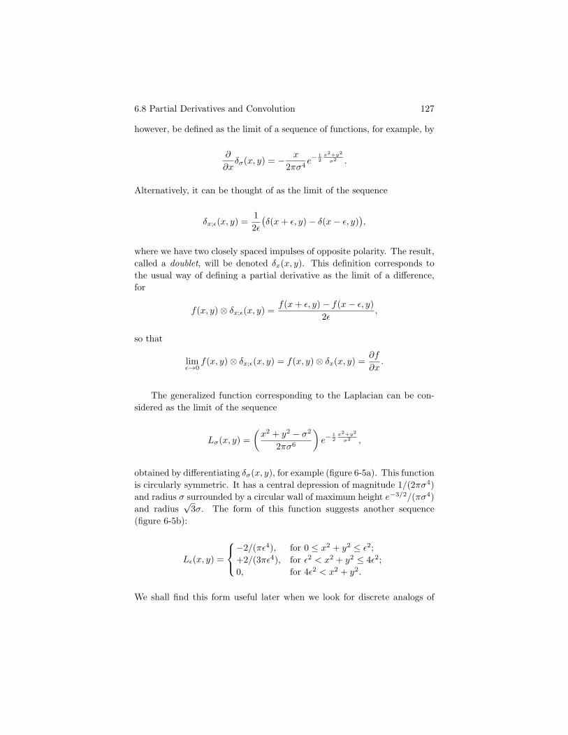
6.8 Partial Derivatives and Convolution 127

however, be defined as the limit of a sequence of functions, for example, by

∂

∂xδσ(x, y) = − x

2πσ4 e− 12

x2+y2

σ2 .

Alternatively, it can be thought of as the limit of the sequence

δx;ε(x, y) =12ε

(δ(x + ε, y) − δ(x − ε, y)

),

where we have two closely spaced impulses of opposite polarity. The result,called a doublet, will be denoted δx(x, y). This definition corresponds tothe usual way of defining a partial derivative as the limit of a difference,for

f(x, y) ⊗ δx;ε(x, y) =f(x + ε, y) − f(x − ε, y)

2ε,

so that

limε→0

f(x, y) ⊗ δx;ε(x, y) = f(x, y) ⊗ δx(x, y) =∂f

∂x.

The generalized function corresponding to the Laplacian can be con-sidered as the limit of the sequence

Lσ(x, y) =(

x2 + y2 − σ2

2πσ6

)e− 1

2x2+y2

σ2 ,

obtained by differentiating δσ(x, y), for example (figure 6-5a). This functionis circularly symmetric. It has a central depression of magnitude 1/(2πσ4)and radius σ surrounded by a circular wall of maximum height e−3/2/(πσ4)and radius

√3σ. The form of this function suggests another sequence

(figure 6-5b):

Lε(x, y) =

−2/(πε4), for 0 ≤ x2 + y2 ≤ ε2;+2/(3πε4), for ε2 < x2 + y2 ≤ 4ε2;0, for 4ε2 < x2 + y2.

We shall find this form useful later when we look for discrete analogs of


these continuous operators.

6.9 Rotational Symmetry and Isotropic Operators 129


6.9 Rotational Symmetry and Isotropic Operators

The Laplacian is the lowest-order linear combination of partial derivativesthat is rotationally symmetric. That is, the Laplacian of a rotated imageis the same as the rotated Laplacian of an image. Conversely, if we rotatean image, take the Laplacian, and rotate it back, we obtain the same resultas if we had just applied the Laplacian.

Another second-order operator that is rotationally symmetric is thequadratic variation,

(∂2

∂x2

)2

+ 2(

∂2

∂x∂y

) (∂2

∂y∂x

)+

(∂2

∂y2

)2

.

It is, however, not linear. If we allow nonlinearity, then the lowest-orderrotationally symmetric differential operator is the squared gradient,

(∂

∂x

)2

+(

∂

∂y

)2

.

The Laplacian, the squared gradient, and the quadratic variation are usefulin detecting edges in images, as we shall see in chapter 8.

Rotationally symmetric operators are particularly attractive becausethey treat image features in the same way, no matter what their orientationis. Also, a rotationally symmetric function can be described by a simpleprofile rather than a surface. Finally, the Fourier transform of a rotationallysymmetric function can be computed using a single integral instead of adouble integral, as we show next.

Let us introduce polar coordinates in both the spatial and the frequencydomains (figure 6-6):

x = r cos φ and y = r sin φ,

u = ρ cos α and v = ρ sin α,

so that ux+vy = rρ cos(φ−α). Now, if f(x, y) = f(r), then the transform

F (u, v) =∫ ∞

−∞

∫ ∞

−∞f(x, y)e−i(ux+vy) dx dy,

becomes just

F (ρ) =∫ π

−π

∫ ∞

0rf(r)e−irρ cos(φ−α) dr dφ.


(The r in the integrand is of course just the determinant of the Jacobianof the transformation from Cartesian to polar coordinates.) If we changethe order of integration, then a simple change of variables turns the innerintegral into

∫ π

−π

e−irρ cos φ dφ = 2∫ π

0cos(rρ cos φ) dφ = 2πJ0(rρ),

where J0(x) is the zeroth-order Bessel function. Thus if F (u, v) = F (ρ),then

F (ρ) = 2π

∫ ∞

0rf(r)J0(rρ) dr.

Similarly, one can show that

f(r) =12π

∫ ∞

0ρF (ρ)J0(rρ) dρ.

These two formulae define the Hankel transforms. (The asymmetry can be


traced to our asymmetric definition of the Fourier transform.)



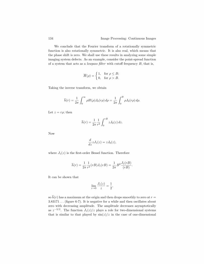
We conclude that the Fourier transform of a rotationally symmetricfunction is also rotationally symmetric. It is also real, which means thatthe phase shift is zero. We shall use these results in analyzing some simpleimaging system defects. As an example, consider the point-spread functionof a system that acts as a lowpass filter with cutoff frequency B, that is,

H(ρ) ={

1, for ρ ≤ B;0, for ρ > B.

Taking the inverse transform, we obtain

h(r) =12π

∫ ∞

0ρH(ρ)J0(rρ) dρ =

12π

∫ B

0ρJ0(rρ) dρ.

Let z = rρ; then

h(r) =12π

1r2

∫ rB

0zJ0(z) dz.

Now

d

dzzJ1(z) = zJ0(z),

where J1(z) is the first-order Bessel function. Therefore

h(r) =12π

1r2 (rB)J1(rB) =

12π

B2 J1(rB)(rB)

.

It can be shown that

limz→0

J1(z)z

=12,

so h(r) has a maximum at the origin and then drops smoothly to zero at r =3.83171 . . . (figure 6-7). It is negative for a while and then oscillates aboutzero with decreasing amplitude. The amplitude decreases asymptoticallyas z−3/2. The function J1(z)/z plays a role for two-dimensional systemsthat is similar to that played by sin(z)/z in the case of one-dimensional


systems.


6.10 Blurring, Defocusing, and Motion Smear 137

It should be apparent, by the way, that a filter with a sharp cutoff willproduce oscillatory responses, or “ringing” effects in the spatial domain(sometimes referred to as Gibbs’s phenomena). In many cases a filter witha more gradual rolloff is better, since it suffers less from these overshootphenomena. A Gaussian filter, for example, has a very smooth rolloff thatextends over a considerable frequency band. It does not introduce anyspurious inflections into the filtered image.

6.10 Blurring, Defocusing, and Motion Smear

In a typical imaging system we find that the rays that would be focusedat a single point in an ideal system are, in fact, slightly spread out. Thisblurring of the image can take various forms, but it can sometimes bemodeled by a Gaussian point-spread function,

h(x, y) =1

2πσ2 e− 12

x2+y2

σ2 ,

with unit volume. This is a rotationally symmetric point-spread function,since it depends only on x2 + y2, not on x or y separately. We can computeits Fourier transform using the Hankel transform formula.

Note, however, that the Gaussian happens to be separable into theproduct of a function of x and a function of y. So another approach maybe easier:

H(u, v) =∫ ∞

−∞

∫ ∞

−∞

12πσ2 e− 1

2x2+y2

σ2 e−i(ux+vy) dx dy

=1√2πσ

∫ ∞

−∞e− 1

2 ( xσ )2

e−iux dx1√2πσ

∫ ∞

−∞e− 1

2 ( yσ )2

e−ivy dy.

The first integral on the right-hand side equals

1√2πσ

∫ ∞

−∞e− 1

2 ( xσ )2

cos(ux) dx = σe− 12 u2σ2

.

So finally,H(u, v) = e− 1

2 (u2+v2)σ2,

which is rotationally symmetric, as expected.We note that low frequencies are passed unattenuated, while higher

frequencies are reduced in amplitude, significantly so for frequencies aboveabout 1/σ. Now σ is a measure of the size of the original point-spreadfunction; therefore, the larger the blur, the lower the frequencies that are


attenuated. This is an example of the inverse relationship between scalechanges in the spatial domain and corresponding scale changes in the fre-quency domain. In fact, if r is a measure of the radius of a blur in thespatial domain, and ρ is a measure of the radius of its transform, then r ρ


is constant.



One way to blur an image is to defocus it (figure 6-1). In this case thepoint-spread function is a little pillbox, as can be seen by considering thecone of light emanating from the lens with its vertex at the focal point.(This point does not lie on the image plane, but slightly in front of orbehind it.) The image plane cuts this cone in a circle. Within the circle,brightness is uniform (figure 6-8), so we have

h(x, y) ={

1/(πR2), for x2 + y2 ≤ R2;0, for x2 + y2 > R2.

Here

R =12

d

f ′ e,

where d is the diameter of the lens, f ′ the distance from the lens to thecorrectly focused spot, and e the displacement of the image plane. We canapply the Hankel transform formula to obtain

H(ρ) =2

R2

∫ R

0rJ0(rρ) dr = 2

J1(Rρ)(Rρ)

,

using the fact thatd

dzzJ1(z) = zJ0(z),

as noted before. Again, low frequencies are passed unattenuated, whilehigher frequencies are reduced in amplitude, and some are not passed atall. Some are even inverted, since J1(z) oscillates about zero. For frequen-cies for which J1(Rρ) < 0 we find that the brightest parts of the defocusedimage coincide with the darkest parts of the ideal image, and vice versa.Components of the waveform with frequencies for which J1(Rρ) = 0 areremoved completely. Such components cannot be recovered from the de-focused image. As mentioned before, the first zero of the function J1(z)occurs at z = 3.83171 . . . .We observe again the inverse scaling in the spa-tial and frequency domains, since in our case z = Rρ. That is, the largerthe defocus radius R, the lower the frequency ρ for which J1(Rρ) = 0.

Another form of image degradation is due to image motion. This canresult from motion of either the imaging system or the objects being im-aged. In either case an image point is smeared into a line. For convenience,suppose the motion is along the x-axis and the length of the line is 2l. Thenthe point-spread function can be described by the product

hx(x, y) =12l

(u(x + l) − u(x − l)

)δ(y),


where u(z) is the unit step function, as before. In this case the point-spreadfunction is not rotationally symmetric. Its Fourier transform can be foundas follows:

H(u, v) =∫ ∞

−∞

12l

(u(x − l) − u(l − x)

)e−iux dx

∫ ∞

−∞δ(y)e−ivy dy,

or

H(u, v) =12l

∫ l

−l

e−iux dx,

so that

H(u, v) =sin(ul)

ul.

The argument can easily be extended to motion in any direction. Onceagain, low frequencies are hardly affected, while higher ones are attenuated.Waves at some frequencies are inverted, and those for which ul = πk, wherek is an integer, are completely suppressed. Waves with crests parallel tothe direction of motion are not affected at all, of course.

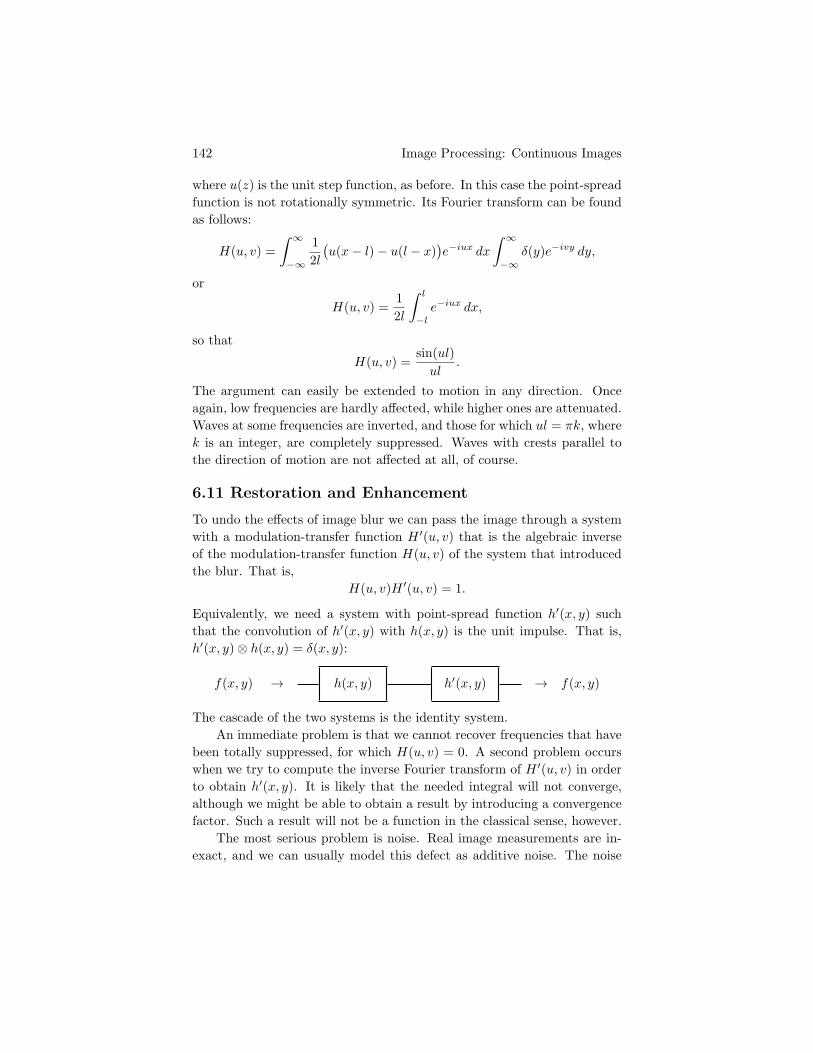
6.11 Restoration and Enhancement

To undo the effects of image blur we can pass the image through a systemwith a modulation-transfer function H ′(u, v) that is the algebraic inverseof the modulation-transfer function H(u, v) of the system that introducedthe blur. That is,

H(u, v)H ′(u, v) = 1.

Equivalently, we need a system with point-spread function h′(x, y) suchthat the convolution of h′(x, y) with h(x, y) is the unit impulse. That is,h′(x, y) ⊗ h(x, y) = δ(x, y):

f(x, y) → h(x, y) h′(x, y) → f(x, y)

The cascade of the two systems is the identity system.An immediate problem is that we cannot recover frequencies that have

been totally suppressed, for which H(u, v) = 0. A second problem occurswhen we try to compute the inverse Fourier transform of H ′(u, v) in orderto obtain h′(x, y). It is likely that the needed integral will not converge,although we might be able to obtain a result by introducing a convergencefactor. Such a result will not be a function in the classical sense, however.

The most serious problem is noise. Real image measurements are in-exact, and we can usually model this defect as additive noise. The noise

6.11 Restoration and Enhancement 143

at one image point is typically independent of, and thus uncorrelated with,the noise at all other image points. It can be shown that this implies thatthe noise has a flat spectrum: The noise power in any given region of thefrequency domain is as large as that in any other region with same area.

Unfortunately, the noise we are concerned with here is introduced af-ter the blurring. The effect is that strongly attenuated frequencies tendto become submerged in the noise, and when we try to recover them byamplification, we also amplify the noise. This is the basic limitation ofimage restoration, and it is due to the fact that, at any given frequency,


we cannot distinguish between signal and noise.

6.11 Restoration and Enhancement 145


One approach to restoration is heuristic. We can design a system thathas a modulation-transfer function approximately equal to the inverse ofthe modulation-transfer function of the blurring system. We place an upperlimit, however, on the amplification. For example,

|H ′(u, v)| = min(

1|H(u, v)| , A

),

where A is the maximum gain. Or more elegantly, we can use somethinglike

H ′(u, v) =H(u, v)

H(u, v)2 + B2 ,

where 1/(2B) is the maximum gain, if H(u, v) is real (figure 6-9).

6.12 Correlation and the Power Spectrum

When images are processed, it is at times useful to correlate them. Inthis way we can tell, for example, how similar two brightness patterns are(figure 6-10). The crosscorrelation of a(x, y) and b(x, y) is defined by

a � b =∫ ∞

−∞

∫ ∞

−∞a(ξ − x, η − y) b(ξ, η) dξ dη.

We shall use the notation φab(x, y) for this integral. Note the similarity tothe definition of convolution. The only difference lies in the arguments ofthe first function in the integrand. Here a(ξ, η) is simply shifted by (x, y)before being multiplied by b(ξ, η). In convolution the first function is also“flipped over” in x and y:

a ⊗ b =∫ ∞

−∞

∫ ∞

−∞a(x − ξ, y − η) b(ξ, η) dξ dη.

If b(x, y) = a(x, y), the result is called the autocorrelation. The autocor-relation of a function is symmetric, that is, φaa(−x,−y) = φaa(x, y). Itcan be shown that the autocorrelation of any function has a maximum at(x, y) = (0, 0), so that

φaa(0, 0) ≥ φaa(x, y) for all (x, y).

If b(x, y) is a shifted version of a(x, y),

b(x, y) = a(x − x0, y − y0),

6.12 Correlation and the Power Spectrum 147

then a similar maximum will occur for the appropriate value of shift. Thatis,

φab(x0, y0) ≥ φab(x, y) for all (x, y).

Note that there can be other maxima, particularly if a(x, y) is periodic.Nevertheless, when b(x, y) is approximately equal to a shifted version of


a(x, y), then the shift can be estimated by looking for maxima in φab.

6.12 Correlation and the Power Spectrum 149


The Fourier transforms of the crosscorrelations and autocorrelationsare often informative. They are called power spectra for reasons that willbecome apparent, and they are denoted Φab(u, v) and Φaa(u, v), respec-tively. If the Fourier transform of a(x, y) is A(u, v), then

Φaa(u, v) = |A(u, v)|2 = A∗(u, v)A(u, v),

where A∗(u, v) is the complex conjugate of A(u, v). Thus Φaa is alwaysreal, a property that can also be deduced from the symmetry of φaa andthe fact that the transform of a(−x,−y) is A∗(u, v). In any case, for smallδu and δv,

Φaa(u, v) δu δv

is the power in the rectangular region of the frequency domain lying be-tween u and u + δu and v and v + δv. This explains the origin of the termpower spectrum.

Even when the Fourier transform of a(x, y) does not converge, its powerspectrum may still exist. It should also be noted that A(u, v) uniquelyspecifies a(x, y) via the inverse Fourier transform, but there is no uniquefunction corresponding to a given Φaa(u, v). Infinitely many functions havethe same autocorrelation and thus the same power spectrum. The powerspectrum does not change, for example, when an image is translated, sinceonly the phase of the Fourier transform is changed. If an object can berecognized from the power spectrum of an image, then it can be recognizedindependently of its position. Great hope was held out at one time, forthis reason, that Fourier transform methods would be important in solvingrecognition problems. Unfortunately, such methods only work when theobject is alone in the image and does not rotate or change size. Moreover,as we have seen, the power spectra of different objects may be the same.

Random noise provides another interesting illustration. The Fouriertransform of an image in which each point has independent random noisewith mean zero and standard deviation σ is a similar random image withmean zero and standard deviation 2πσ. The average of the power spectraof an infinite number of such random images tends to the constant (2πσ)2

at all frequencies.

6.13 Optimal Filtering and Noise Suppression

The next section, dealing with optimal filtering, requires some patiencewith nontrivial mathematical manipulations. The hasty reader may chooseto skip it on first reading without serious loss of continuity. It may be

6.13 Optimal Filtering and Noise Suppression 151

worthwhile returning to this section later, however, since it is the first placein this book where we introduce the tools of the calculus of variations.

Suppose that we are given the sum of the signal b(x, y) and the noisen(x, y). Our task is to recover, as best we can, the signal b(x, y). The mea-sure of how well we succeed will be the integral of the square of the differ-ence between the output o(x, y) and the desired signal d(x, y) (figure 6-11).Usually d(x, y) is just b(x, y). We choose to minimize the integral of thesquare of the error because it leads to tractable mathematics. (This, ofcourse, is the real reason for the popularity of least-squares methods in


general.)



We have to minimize the squared error

E =∫ ∞

−∞

∫ ∞

−∞

(o(x, y) − d(x, y)

)2dx dy.

If we are going to use a linear system for the filtering operation, we cancharacterize the system by means of its point-spread function h(x, y). Theinput to the system is

i(x, y) = b(x, y) + n(x, y),

and the output iso(x, y) = i(x, y) ⊗ h(x, y).

So

E =∫ ∞

−∞

∫ ∞

−∞

(o2(x, y) − 2o(x, y)d(x, y) + d2(x, y)

)dx dy.

Since o2 = (i ⊗ h)2,

o2(x, y) =∫ ∞

−∞

∫ ∞

−∞i(x − ξ, y − η)h(ξ, η) dξ dη

×∫ ∞

−∞

∫ ∞

−∞i(x − α, y − β)h(α, β) dα dβ,

and so∫ ∞

−∞

∫ ∞

−∞o2(x, y) dx dy

=∫ ∞

−∞

∫ ∞

−∞

∫ ∞

−∞

∫ ∞

−∞φii(ξ − α, η − β)h(ξ, η)h(α, β) dξ dη dα dβ,

where φii(x, y) is the autocorrelation of i(x, y). Moreover,

o(x, y)d(x, y) =∫ ∞

−∞

∫ ∞

−∞i(x − ξ, y − η)h(ξ, η)d(x, y) dξ dη,

and so∫ ∞

−∞

∫ ∞

−∞o(x, y)d(x, y) dx dy =

∫ ∞

−∞

∫ ∞

−∞φid(ξ, η)h(ξ, η)) dξ dη,

where φid(x, y) is the crosscorrelation of i(x, y) and d(x, y). Finally weneed ∫ ∞

−∞

∫ ∞

−∞d2(x, y) = φdd(0, 0),


where φdd(x, y) is the autocorrelation of d(x, y). We can now rewrite theexpression for the error term to be minimized in the form

E =∫ ∞

−∞

∫ ∞

−∞

∫ ∞

−∞

∫ ∞

−∞φii(ξ − α, η − β)h(ξ, η)h(α, β) dξ dη dα dβ

− 2∫ ∞

−∞

∫ ∞

−∞φid(ξ, η)h(ξ, η) dξ dη + φdd(0, 0).

This expression is to be minimized by finding the point-spread functionh(x, y). This is a problem in the calculus of variations. (The calculus ofvariations is covered in more detail in the appendix.) We shall attack theproblem using the basic method of that speciality. In the typical calculusproblem we look for a parameter value that results in a stationary value ofa given function. In the problem here, we are looking instead for a functionthat leads to a stationary value of a given functional. A functional is anexpression that depends on a function, as, for example, E above dependson h(ξ, η).

Suppose that h(x, y) gives the minimum value of E, and let δh(x, y)be an arbitrary function used to modify h(x, y). Then h(x, y) + ε δh(x, y)will give a value that cannot be less than E, no matter what δh(x, y) is.Let the value be E + δE. If we are truly at a minimum, then

limε→0

∂

∂ε(E + δE) = 0 for all δh(x, y).

If this were not the case, we could reduce E by adding a small multipleof δh(x, y) to h(x, y), thus contradicting the assumption that h(x, y) isoptimal. Now

limε→0

∂

∂ε(E + δE)

= 2∫ ∞

−∞

∫ ∞

−∞

∫ ∞

−∞

∫ ∞

−∞φii(ξ − α, η − β)h(ξ, η)δh(α, β) dξ dη dα dβ

− 2∫ ∞

−∞

∫ ∞

−∞φid(ξ, η)δh(ξ, η) dξ dη,

or

limε→0

∂

∂ε(E + δE)

= −2∫ ∞

−∞

∫ ∞

−∞

[φid(ξ, η) −

∫ ∞

−∞

∫ ∞

−∞φii(ξ − α, η − β)h(α, β) dα dβ

]


× δh(ξ, η) dξ dη.

If this is to be zero for all δh(x, y), then the bracketed expression must bezero, or

φid(ξ, η) =∫ ∞

−∞

∫ ∞

−∞φii(ξ − α, η − β)h(α, β) dα dβ,

that is, perhaps surprisingly,

φid = φii ⊗ h .

This simple equation for h(x, y) can be solved by taking the Fourier trans-form,

Φid = HΦii,

where Φii and Φid are the power spectra. The power spectra are thus allwe need to know to design the image-restoring system under the given as-sumptions. The same system will be optimal for a large class of images, notjust a single one. (It would, of course, not be of much interest otherwise.)

As an example, consider a system designed to suppress noise, that is,a system that takes the sum of the image b(x, y) and the noise n(x, y) andproduces an output o(x, y) that is as close as possible, in the least-squaressense, to the original image b(x, y). Here d(x, y) = b(x, y) and

i(x, y) = b(x, y) + n(x, y).

SoΦid = Φbb + Φnb,

andΦii = Φbb + Φbn + Φnb + Φnn,

as can be seen by noting the definitions of Φii and Φid. We now assumethat the noise is not correlated to the signal, so that Φbn = Φnb = 0. Then

H =Φid

Φii=

Φbb

Φbb + Φnn=

11 + Φnn/Φbb

.

It is clear what the optimal system is doing. In parts of the spectrum wherethe signal-to-noise ratio, Φbb/Φnn, is high, the gain is almost unity; in partswhere the noise dominates, the gain is very low, approximately Φbb/Φnn,which is just the signal-to-noise ratio.


Now consider the case where the signal b(x, y) is passed through asystem with point-spread function h(x, y) before the noise n(x, y) is added.The result,

i = b ⊗ h + n,

is to be passed through a system with point-spread function h′(x, y). Theoutput

o = i ⊗ h′

should be as close as possible to the original image b(x, y), in the least-squares sense. Here d(x, y) = b(x, y), so that

Φid = HΦbb + Φnb

andΦii = H2Φbb + H(Φnb + Φbn) + Φnn.

Assuming that the noise is not correlated with the signal, we have

H ′ =Φid

Φii=

HΦbb

H2Φbb + Φnn.

If the signal-to-noise ratio is high in a particular part of the spectrum, then

H ′ ≈ 1H

there, while gain is limited to about H(Φbb/Φnn) in parts where Φnn >

|H|2 Φbb. Note the similarity of this result to that derived heuristicallyearlier.

Finally, it may be instructive to consider the optimal filter for estimat-ing a processed version of the image rather than the image itself. Supposewe want the least-squares estimate of

d(x, y) = b(x, y) ⊗ p(x, y),

where p(x, y) is the point-spread function of a processing filter. Then

φid = i � d = i � (b ⊗ p) = (i � b) ⊗ p = φib ⊗ p,

so thatΦid = Φib P,

where P (u, v) is the Fourier transform of p(x, y). Thus

H ′ =Φid

Φii=

Φib

ΦiiP.


The optimal filter is just the cascade of the optimal filter for recovering theimage b(x, y) and the processing filter P (u, v). We do not need anythingelse.

We should note at this point that the design of the optimal filter hereis much simpler than in the one-dimensional situation. This is because theimpulse response in the one-dimensional case must be one-sided, since asystem cannot anticipate its input. Limitations in the time domain do nottranslate easily into understandable limitations in the frequency domain.For example, it is hard to express the constraint that f(t) = 0 for t < 0 interms of F (ω), the Fourier transform of f(t). Fortunately, there is no suchproblem in the case of images, since the support of a point-spread functioncan extend in all directions from the origin. The support of a function isthe region over which it is nonzero.

6.14 Image Models

In order to apply the optimal filtering methods, we must estimate thepower spectra of the images to be processed. Looking at the spectra of afew “typical” images will quickly persuade you that most of the energy isconcentrated at the lower frequencies. It is useful to know about this falloffwith frequency since it helps separate the desired signal from the noise,which has a flat spectrum. The observed falloff in power with frequency is,in part, due to the fact that many objects or parts of objects are opaqueand have nearly uniform brightness. The corresponding image patches areseparated by discontinuities along edges where objects occlude one another.

A full discussion of image models lies beyond the scope of this book,but we can get a rough idea by considering a simple rectangular patch

f(x, y) ={

1, for |x| ≤ W and |y| ≤ H;0, for |x| > W or |y| > H.

The Fourier transform is

F (u, v) = WHsin(uW )

uW

sin(vH)vH

.

Shifting the patch just changes the phase, not the magnitude, of the trans-form. Ignoring the oscillations, we see that the transform falls off as 1/(uv).Thus, depending on the direction we choose in the frequency domain, itfalls off as 1/ρ or 1/ρ2 with distance ρ from the origin.

6.14 Image Models 159

Another useful component of an image model might be the “pillbox”patch,

f(r) ={

1, for r ≤ R;0, for r > R.

The transform in this case is

F (ρ) = 2R2 J1(ρR)(ρR)

.

For large arguments, J1(z) behaves like

√2πz

sin(z − π/4),

so that, if we ignore the oscillations, F (ρ) falls off as 1/ρ3/2 for large ρ.Image models containing polygonal or circular patches tend to have

power spectra falling off as some power of frequency. At higher frequen-cies real images fall off even more rapidly, due to the resolution limits ofthe optical system. In telescopes, for example, there is an absolute cutofffrequency, determined by the ratio of the aperture diameter to the wave-length of light, above which there is no transmission at all. Microscopeshave a similar absolute limitation determined by the numerical aperture ofthe objective and the wavelength of light.

A different application of the observation that most power in images isconcentrated at low frequencies can be found in image reproduction. Meth-ods for displaying images, such as the printing of halftones, photographicreproduction, and television, have limited dynamic range; that is, they canonly show a certain range of gray-level values. In terms of the quality ofreproduction, what we are interested in is the ratio of the brightest to thedarkest reproducible gray-level. One important consideration in display-ing images is that small brightness differences be perceptible. Even largedifferences in brightness between adjacent regions may not be noticeable ifthe regions are themselves very bright. What is important is the relativesize of the brightness difference, that is, the ratio of the difference to thesmaller of the two. It is for this reason that dynamic range is measuredby the ratio of the brightest to the darkest level that can be reproduced,rather than the difference.

The dynamic range of color transparencies can be over a hundred toone, while that of newsprint is often not much more than ten to one. Nat-ural images tend to have large dynamic ranges. Usually a compromise has


to be struck when they are to be reproduced. If we try to impose the vari-ation in image brightness unchanged onto the medium, the brightest andthe darkest areas will not be reproduced properly. To avoid losing detailin the highlights and shadows due to saturation, we have to compress thedynamic range.

A power function can do this compression. If the brightness of thereproduction is b′(x, y) and that of the original is b(x, y), then

b′(x, y) =(b(x, y)

)γ,

where 0 < γ < 1. Such reproductions are generally acceptable, althoughbarely perceptible brightness differences in the original will be impercepti-ble in the reproduction.

Another approach is to take advantage of the fact that images usuallycontain large low-frequency components. A filter that attenuates low fre-quencies can be devised by subtracting from the image a smoothed versionof the image. Such a filter will tend to reduce the dynamic range. Anexample is provided by a filter with a point-spread function

h(x, y) = δ(x, y) − k

2πσ2 e− 12

x2+y2

σ2

for 0 < k < 1. The modulation-transfer function of this filter is

H(u, v) = 1 − ke− 12 (u2+v2)σ2

.

Other smoothing functions can be used. A photographic technique forachieving a similar effect is called unsharp masking. Here an out-of-focusimage is “subtracted,” in part, from the original. Note that, in this case,sharp edges are reproduced with their full contrast. We have to be careful inapplying this process, however, since the brightness values in the image areshifted around and spurious changes in the appearance of the objects mayresult. As we shall see later, the brightness values are used in recoveringsurface shape, for example.

6.15 References

The classic reference on image processing is Digital Image Processing byPratt [1978]. The first few chapters of Digital Picture Processing by Rosen-feld & Kak [1982] also provide an excellent introduction to the subject.Much of the two-dimensional analysis is a straightforward extension of theone-dimensional case aptly described in Signals and Systems by Oppenheim& Willsky [1983] and Circuits, Signals, and Systems by Siebert [1986]. The

6.16 Exercises 161

underlying theory of the Fourier transform is given in the standard referenceThe Fourier Transform and Its Applications by Bracewell [1965, 1978]. Anenjoyable discussion of generalized functions appears in Lighthill’s Intro-duction to Fourier Analysis and Generalised Functions [1978]. Even moredetail can be found in Generalized Functions: Properties and Operationsby Gel’fand & Shilov [1964]. Few texts explicitly discuss convergence fac-tors; one that does is Summable Series and Convergence Factors by Moore[1966].

The basic work on optimal filtering is due to Wiener. He uses a de-lightfully symmetric definition of the Fourier transform in Extrapolation,Interpolation, and Smoothing of Stationary Time Series with EngineeringApplications [1966]. The optimal filter is derived using the methods ofthe calculus of variations, for which volume I of Methods of MathematicalPhysics by Courant & Hilbert [1953] may be the best reference. Imagemodels are discussed in Pattern Models by Ahuja & Schachter [1983].

Image processing is a relatively old field that matured more than tenyears ago. A survey of early work on image processing is provided byHuang, Schreiber, & Tretiak [1971]. The classic application of imageprocessing method has been in improving image quality, as discussed bySchreiber [1978].

Detailed structure in an image that is too fine to be resolved, yet coarseenough to produce a noticeable fluctuation in the gray-levels of neighboringpicture cells, constitutes texture. (Note that there are other notions ofwhat is meant by the term texture.) Texture may be periodic, nearlyperiodic, or random. There has been work devoted to the derivation oftexture measures that allow classification. Other efforts are directed at thesegmentation of images into regions of differing texture, as in the work ofBajcsy [1973] and Ehrich [1977]. Methods for the analysis of gray-levelco-occurrence histograms have found application in this domain. Anotherapproach depends on the appearance of peaks in the frequency domain.Ahuja & Rosenfeld [1981] study the relationship of mosaic image modelsto the notion of texture. Further references relating to image processingwill be given at the end of the next chapter.

6.16 Exercises

6-1 Find k(σ) such that the family of functions

δσ(x, y) = k(σ) e− 1

2x2+y2

σ2

defines the unit impulse δ(x, y) as σ → 0.


6-2 Consider the family of functions

Lδ(x, y) =

{a, for r ≤ δ;b, for δ < r ≤ 2δ;0, for 2δ < r;

where r =√

x2 + y2. For what values of a and b does this family define thegeneralized function that corresponds to the Laplacian? That is, when is thelimit of the convolution of Lδ(x, y) with some given function f(x, y) equal to∇2f(x, y)? Hint: It may help to apply the operator to the test function

14(x2 + y2),

whose Laplacian is known to be equal to one.

6-3 Show that if f(x, y) is separable into a product of a function of x and afunction of y, its Fourier transform F (u, v) is also separable into a function of u

and a function of v.

6-4 Show that if f(x, y) ≥ 0 for all x and y, then F (0, 0) ≥ |F (u, v)| for all u

and v. When is F (0, 0) = F (u, v)?

6-5 Usually the point-spread function h(x, y) of an operator used for smoothingoperations is largest at the origin, (x, y) = (0, 0), positive everywhere, and diesaway as x and y tend to infinity. It can be conveniently thought of as a massdistribution. Without loss of generality we shall assume that the center of massof this distribution lies at the origin. We need to be able to say how “spreadout” such a distribution is. The radius of gyration of a mass distribution is thedistance from its center of mass at which a point of equal mass would have tobe placed in order for it to have the same inertia as the given distribution. (Theinertia of a point mass is the product of the square of the distance from the origintimes the mass.)

The total mass M of a distribution h(x, y) is just

M =∫ ∞

−∞

∫ ∞

−∞h(x, y) dx dy,

while the radius of gyration R is defined by∫ ∞

−∞

∫ ∞

−∞r2h(x, y) dx dy = R2

∫ ∞

−∞

∫ ∞

−∞h(x, y) dx dy = M R2,

where r2 = x2 + y2.

6.16 Exercises 163

(a) Find the radius of gyration of a pillbox defined by

bV (x, y) =

{1/(πV 2), for r ≤ V ;0, for r > V .

(b) Find the radius of gyration of the Gaussian

Gσ(x, y) =1

2πσ2 e− 1

2x2+y2

σ2 .

Note that the distributions in (a) and (b) both have “unit mass” and that it mayhelp to convert the required integrals to polar coordinates.

(c) Show that the mass of the convolution of two smoothing functions is theproduct of the masses of the two functions. Also show that, when smoothingfunctions are convolved, their gyration radii squared add. That is, if f =g ⊗ h, then R2

f = R2g + R2

h, where Rf , Rg, and Rh are the radii of gyrationof f , g, and h, respectively.

(d) When a rotationally symmetric smoothing function is convolved with itselfmany times, it becomes indistinguishable from the Gaussian. Suppose thatthe pillbox is convolved with itself n times. What is the value of σ of theapproximating Gaussian?

6-6 Show that a�(b⊗c) = (a�b)⊗c, where � denotes correlation and ⊗ denotesconvolution.

6-7 The modulation-transfer function of an optical telescope is A(u, v) =P (u, v) ⊗ P (u, v), where P (u, v) is the rotationally symmetric lowpass filter

P (u, v) =

{1, for u2 + v2 ≤ ω2;0, for u2 + v2 > ω2,

for some ω, where ω is a function of the wavelength of light and the size of thecollecting optics.

(a) Find A(u, v). Hint: What is the overlap between two disks of equal diameterwhen their centers are not aligned?

(b) What is the corresponding point-spread function? Hint: What does multi-plication in the frequency domain correspond to in the spatial domain?

6-8 Consider a system that blurs images according to a Gaussian point-spreadfunction with standard deviation σ. Suppose that the noise power spectrum isflat with power N2, the signal power spectrum is also flat with power S2, andthat S2 > N2. (Noise is added to the image after blurring.)


(a) Sketch the modulation-transfer function of the optimal filter for deblurringthe image.

(b) What is the low-frequency response?

(c) What frequency is maximally amplified?

(d) What is the maximal gain?

6-9 It is difficult to measure the point-spread function of an optical system di-rectly. Instead, we usually image a sharp edge between two regions with differentbrightnesses. In this fashion we obtain the edge-spread function.

(a) How would you obtain the line-spread function l(x) from the response e(x)to a unit step edge? The line-spread function is the response of the systemto an impulsive line.

(b) Show that l(x) is related to the point-spread function h(r) by

l(x) = 2∫ ∞

x

r√r2 − x2

h(r) dr.

This is the definition of the Abel transform. Here l(x) is the Abel transformof h(r). Assume that the point-spread function is rotationally symmetric.

(c) Show that the Abel transform obeys the relationships∫ ∞

−∞l(x) dx = 2π

∫ ∞

0h(r) r dr and l(0) = 2

∫ ∞

0h(r) dr.

(d) How would you recover the point-spread function from the measured line-spread function? Show that

h(r) = − 1π

∫ ∞

r

l′(x)√x2 − r2

dx = − 1π

∫ ∞

r

√x2 − r2 d

dx

(l′(x)

x

)dx,

where l′(x) is the derivative of l(x) with respect to x. This is the inverseAbel transform.

6-10 A rotationally symmetric function f(x, y) depends only on the radius r

and does not depend on the polar angle θ, where

r =√

x2 + y2 and θ = tan−1(y/x).

Show that the Gaussian is the only rotationally symmetric function that can bedecomposed into the product of a function of x and a function of y; that is,f(x, y) = g(x)h(y). Hint: First prove that f(x, y) is rotationally symmetric ifand only if

1x

∂f

∂x=

1y

∂f

∂y.

6.16 Exercises 165

You can then easily prove that, for some constant c,

dg

dx= c x g(x) and

dh

dy= c y h(y).

Documents

6 Image Processing: Continuous Imagespeople.csail.mit.edu/bkph/courses/papers/RoVis/ch6_FT_continuous.… · 6 Image Processing: Continuous Images It is often useful to transform