Embed Size (px)
Citation preview
On the Theory of the Second-Order Soundfield Microphone Philip Cotterell
108
6: The Second-Order Soundfield Microphone
Gerzon stated [40] that a second-order soundfield microphone may be constructed “...using
twelve small cardioid or hypercardioid capsules mounted to form the faces of a regular
dodecahedron having a small diameter ... the second-harmonic aspects of the directional
pickup can be derived from these by techniques similar to the Blumlein difference
technique.” Since the dodecahedron is the simplest regular polyhedron with nine or more
faces, so a dodecahedral array is the simplest arrangement of microphones from which the
nine independent signals comprising the second-order B-format set can be obtained.
6.1: Geometry of the Dodecahedron
It is desirable to maximise the degree of symmetry present in the coefficients of the A-B
matrix, since this simplifies the mathematical treatment (and will also simplify the eventual
implementation).
The symmetry which is apparent in the coefficients of the A-B matrix in the case of the
first-order soundfield microphone is related to the symmetry of the tetrahedron; specifically,
to the presence of C3 operations in the group of rotational symmetries of the tetrahedron [61].
Each C3 axis passes through a vertex and the centroid of the opposite face of the tetrahedron.
Rotation by 120° about one of these axes has the effect of taking )cos()cos( φθ to
)cos()sin( φθ (or vice versa) and etc.; i.e., of inducing a cyclic permutation of the polar
patterns associated with the first-order spherical harmonic component signals. The same
rotation interchanges the faces of the tetrahedron in a corresponding manner.
Such C3 operations are also present in the group of symmetries of the dodecahedron. To
maximise the symmetry in the A-B matrix coefficients for the second-order soundfield
microphone, the dodecahedral capsule array is oriented such that appropriate C3 axes (which
pass through two diametrically opposed vertices) are aligned with those of the tetrahedral
first-order soundfield microphone array.
By inspection, two orientations which satisfy this criterion may be identified; selection
between these is arbitrary. The chosen orientation is such that the highest part of the
On the Theory of the Second-Order Soundfield Microphone Philip Cotterell
109
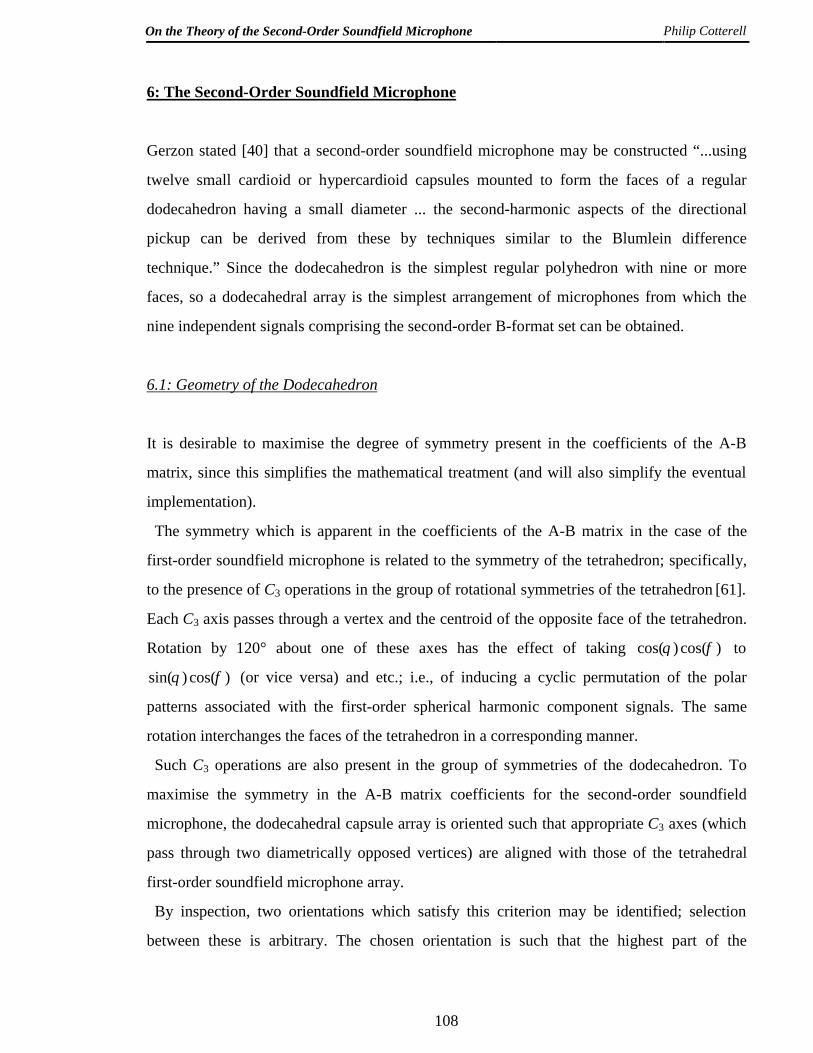
dodecahedron is an edge running front-back, and the front-most part is a horizontal edge - see
figure 6.1.
Figure 6.1: Orientation of Dodecahedron
(viewed from centre-front direction)
Two faces, having the front-most edge in common, point symmetrically up and down, with
no left / right component in their orientation; these faces are conveniently labelled FU and
FD. Their (outward) unit surface normal vectors are
=
z
x
FU 0u (6.1)
and
On the Theory of the Second-Order Soundfield Microphone Philip Cotterell
110
−=
z
x
FD 0u (6.2)
The cosine of the angle between vectors normal to two adjacent faces of a regular polyhedron
is equal to the cosine of the dihedral angel at each edge of that polyhedron; hence, the scalar
product of FUu and FDu is equal to the cosine of the dihedral angle at the edges of a regular
dodecahedron.
Now, for any regular polyhedron,
( )( )
= −
f
vd e
eππ
ϑsincos
sin2 1 (6.3)
where dϑ is the dihedral angle, fe is the number of edges around each face, and ve is the
number of edges which meet at each vertex [66]. Rearranging gives
( )( )f
vd
ee
ππϑ
sincos
2sin =
(6.4)
For a dodecahedron, 3=ve and ;5=fe hence
55
2
55241
21
)5/sin()3/cos(
2sin
−=
−=
=
ππϑd
(6.5)
Now since, for any angle ,ϕ
)(sin1)cos( 2 ϕϕ −±= (6.6)
On the Theory of the Second-Order Soundfield Microphone Philip Cotterell
111
so we may use the trigonometric “double angle” identity for sines to obtain
( )10
1553
555322
5553
55
22
5521
55
22
2sin1
2sin2
2cos
2sin2)sin(
2
+−=
−−
=
−−
−=
−−
−=
−
=
=
dd
ddd
ϑϑ
ϑϑϑ
(6.7)
where the positive square root is taken in the substitution from equation (6.6) because the
dihedral angle must by definition be less than 180°. We can now find the cosine of the
dihedral angle:
( )
( )( )
51102
10526531
1051531
)(sin1)cos(2
2
=
=
+−−=
+−−=
−= dd ϑϑ
(6.8)
where the positive square root is taken since (by inspection) the angle in question is less than
90°.
We can now determine the values of the elements of FUu and .ˆ FDu Since they are unit
vectors,
On the Theory of the Second-Order Soundfield Microphone Philip Cotterell
112
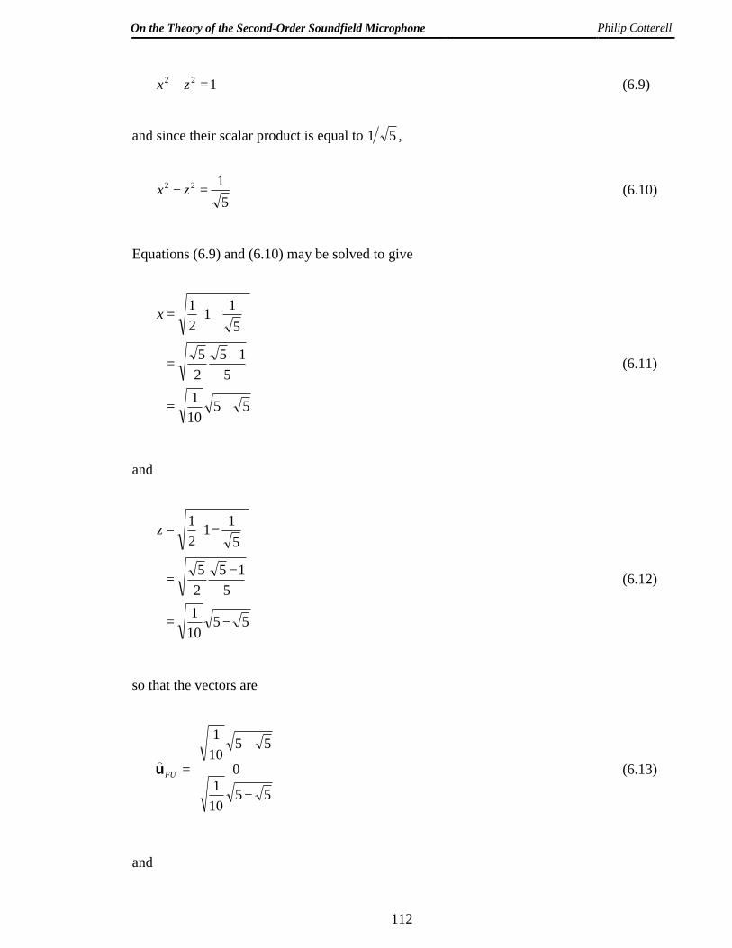
122 =+ zx (6.9)
and since their scalar product is equal to ,51
5122 =− zx (6.10)
Equations (6.9) and (6.10) may be solved to give
55101
515
25
511
21
+=
+=
+=x
(6.11)
and
55101
515
25
511
21
−=
−=
−=z
(6.12)
so that the vectors are
−
+
=
55101
0
55101
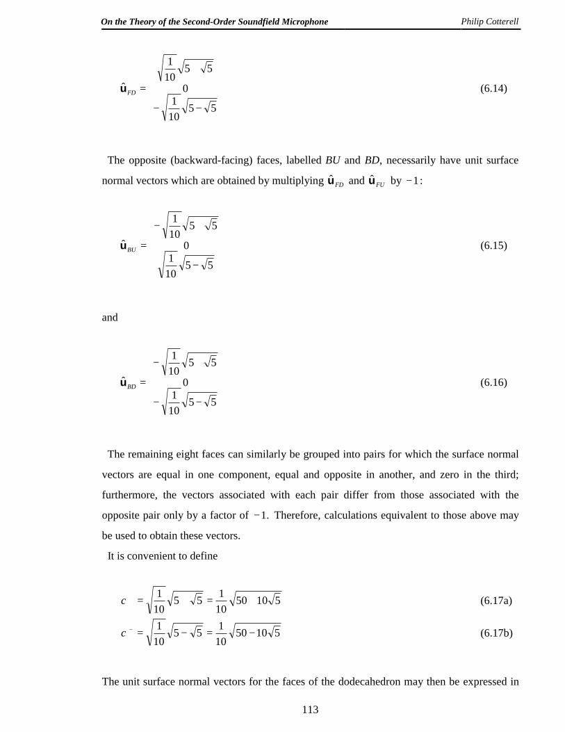
ˆ FUu (6.13)
and
On the Theory of the Second-Order Soundfield Microphone Philip Cotterell
113
−−
+
=
55101
0
55101
ˆ FDu (6.14)
The opposite (backward-facing) faces, labelled BU and BD, necessarily have unit surface
normal vectors which are obtained by multiplying FDu and FUu by :1−
−
+−
=
55101
0
55101
ˆ BUu (6.15)
and
−−
+−
=
55101
0
55101
ˆ BDu (6.16)
The remaining eight faces can similarly be grouped into pairs for which the surface normal
vectors are equal in one component, equal and opposite in another, and zero in the third;
furthermore, the vectors associated with each pair differ from those associated with the
opposite pair only by a factor of .1− Therefore, calculations equivalent to those above may
be used to obtain these vectors.
It is convenient to define
5105010155
101
+=+=+χ (6.17a)
5105010155
101
−=−=−χ (6.17b)
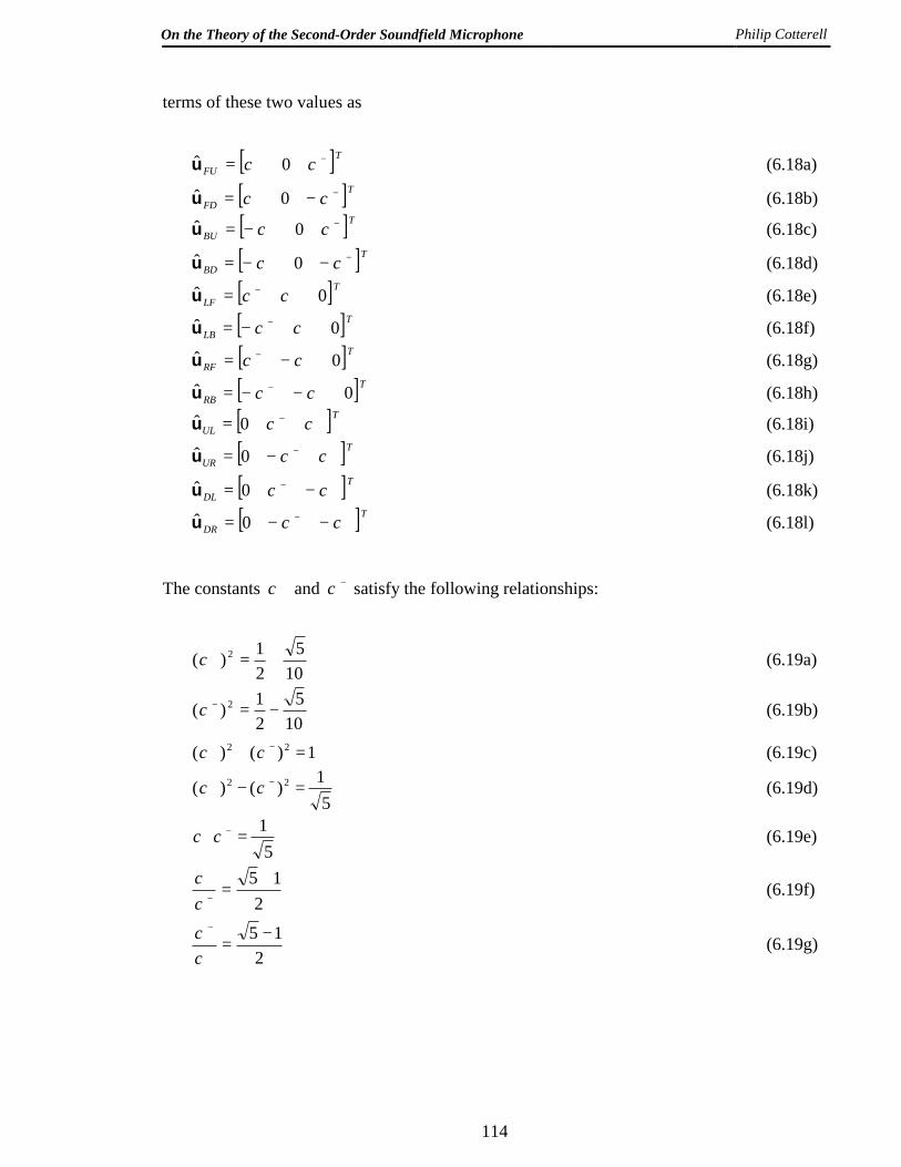
The unit surface normal vectors for the faces of the dodecahedron may then be expressed in
On the Theory of the Second-Order Soundfield Microphone Philip Cotterell
114
terms of these two values as
[ ]TFU
−+= χχ 0u (6.18a)
[ ]TFD
−+ −= χχ 0u (6.18b)
[ ]TBU
−+−= χχ 0u (6.18c)
[ ]TBD
−+ −−= χχ 0u (6.18d)
[ ]TLF 0ˆ +−= χχu (6.18e)
[ ]TLB 0ˆ +−−= χχu (6.18f)
[ ]TRF 0ˆ +− −= χχu (6.18g)
[ ]TRB 0ˆ +− −−= χχu (6.18h)
[ ]TUL
+−= χχ0u (6.18i)
[ ]TUR
+−−= χχ0u (6.18j)
[ ]TDL
+− −= χχ0u (6.18k)
[ ]TDR
+− −−= χχ0u (6.18l)
The constants +χ and −χ satisfy the following relationships:
105
21)( 2 +=+χ (6.19a)
105
21)( 2 −=−χ (6.19b)
1)()( 22 =+ −+ χχ (6.19c)
51)()( 22 =− −+ χχ (6.19d)
51
=−+ χχ (6.19e)
215 +
=−
+
χχ (6.19f)
215 −
=+
−
χχ (6.19g)
On the Theory of the Second-Order Soundfield Microphone Philip Cotterell
115
6.2: Derivation of the A-B Matrix
The method described in Chapter 5 for the derivation of the A-B matrix coefficients in the
case of the first-order soundfield microphone is not applicable when the second-order
soundfield microphone is considered. While we can write equations similar to equations
(5.25) and (5.26) for any of the zeroth-order or first-order signals, this leaves us in each case
with twelve unknown matrix coefficients and only four equations.
A different approach is therefore required. Let a signal H~ be a general linear combination
of the twelve A-format signals:
DRDRDLDLURURULULRBRBRFRF
LBLBLFLFBDBDBUBUFDFDFUFU
vgvgvgvgvgvgvgvgvgvgvgvgH
+++++++++++=~
(6.20)
or, by substituting for each of the A-format signals,
[ ] [ ][[ ] [ ][ ] [ ][ ] [ ][ ] [ ][ ] [ ] ] O
jkrDRDR
jkrDLDL
jkrURUR
jkrULUL
jkrRBRB
jkrRFRF
jkrLBLB
jkrLFLF
jkrBDBD
jkrBUBU
jkrFDFD
jkrFUFU
pebagebag
ebagebag
ebagebag
ebagebag
ebagebag
ebagebagba
GH
DRDL
URUL
RBRF
LBLF
BDBU
FDFU
dudu
dudu
dudu
dudu
dudu
dudu
dudu
dudu
dudu
dudu
dudu
dudu
ˆˆˆˆ
ˆˆˆˆ
ˆˆˆˆ
ˆˆˆˆ
ˆˆˆˆ
ˆˆˆˆ
ˆˆˆˆ
ˆˆˆˆ
ˆˆˆˆ
ˆˆˆˆ
ˆˆˆˆ
ˆˆˆˆ~
⋅⋅
⋅⋅
⋅⋅
⋅⋅
⋅⋅
⋅⋅
⋅++⋅++
⋅++⋅++
⋅++⋅++
⋅++⋅++
⋅++⋅++
⋅++⋅++
=
(6.21)
We may obtain expressions in terms of the matrix coefficients ,FUg ,FDg etc., for the
coefficient of each spherical harmonic component in the Laplace series expansion of H~ by
evaluating the integrals given in equation (2.10). For each B-format signal, we can then
equate these expressions to the desired values of the coefficients; the resulting equations may
then be solved to find the matrix coefficients.
Note that this method is applicable to the second-order component signals; a method
employing a coincident capsule approximation could not be used, since it is the phase
differences between the capsules that allow these signals to be obtained. Furthermore, this
On the Theory of the Second-Order Soundfield Microphone Philip Cotterell
116
approach automatically includes the dependence of the Laplace series coefficients on kr, so
that it is not necessary to determine the frequency response functions separately from the
matrix coefficients.
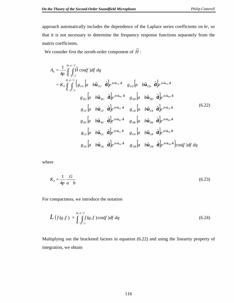
We consider first the zeroth-order component of :~H
[ ] [ ]{[ ] [ ][ ] [ ][ ] [ ][ ] [ ][ ] [ ] } θφφ
θφφπ
π π
π
π π
π
ddebagebag
ebagebag
ebagebag
ebagebag
ebagebag
ebagebagK
ddHA
DRDL
URUL
RBRF
LBLF
BDBU
FDFU
jkrDRDR
jkrDLDL
jkrURUR
jkrULUL
jkrRBRB
jkrRFRF
jkrLBLB
jkrLFLF
jkrBDBD
jkrBUBU
jkrFDFD
jkrFUFU
)cos(ˆˆˆˆ
ˆˆˆˆ
ˆˆˆˆ
ˆˆˆˆ
ˆˆˆˆ
ˆˆˆˆ
)cos(~41
ˆˆˆˆ
ˆˆˆˆ
ˆˆˆˆ
ˆˆˆˆ
ˆˆˆˆ
2
0
2/
2/
ˆˆˆˆ0
2
0
2/
2/0
dudu
dudu
dudu
dudu
dudu
dudu
dudu
dudu
dudu
dudu
dudu
dudu
⋅⋅
⋅⋅
⋅⋅
⋅⋅
⋅⋅
−
⋅⋅
−
⋅++⋅++
⋅++⋅++
⋅++⋅++
⋅++⋅++
⋅++⋅++
⋅++⋅+=
=
∫ ∫
∫ ∫
(6.22)
where
baGK+
=π41
0 (6.23)
For compactness, we introduce the notation
( ) ∫ ∫−
=π π
π
θφφφθφθΛ2
0
2/
2/
)cos(),(),( ddff (6.24)
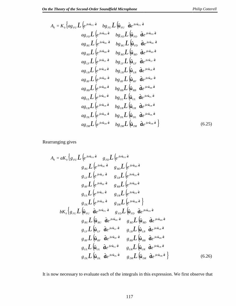
Multiplying out the bracketed factors in equation (6.22) and using the linearity property of
integration, we obtain
On the Theory of the Second-Order Soundfield Microphone Philip Cotterell
117
( ) ( ){( ) ( )( ) ( )( ) ( )( ) ( )( ) ( )( ) ( )( ) ( )( ) ( )( ) ( )( ) ( )( ) ( )}dudu
dudu
dudu
dudu
dudu
dudu
dudu
dudu
dudu
dudu
dudu
dudu
du
du
du
du
du
du
du
du
du
du
du
du
ˆˆˆˆ
ˆˆˆˆ
ˆˆˆˆ
ˆˆˆˆ
ˆˆˆˆ
ˆˆˆˆ
ˆˆˆˆ
ˆˆˆˆ
ˆˆˆˆ
ˆˆˆˆ
ˆˆˆˆ
ˆˆˆˆ00
ˆˆ
ˆˆ
ˆˆ
ˆˆ
ˆˆ
ˆˆ
ˆˆ
ˆˆ
ˆˆ
ˆˆ
ˆˆ
ˆˆ
⋅⋅
⋅⋅
⋅⋅
⋅⋅
⋅⋅
⋅⋅
⋅⋅
⋅⋅
⋅⋅
⋅⋅
⋅⋅
⋅⋅
⋅++
⋅++
⋅++
⋅++
⋅++
⋅++
⋅++
⋅++
⋅++
⋅++
⋅++
⋅+=
DRDR
DLDL
URUR
ULUL
RBRB
RFRF
LBLB
LFLF
BDBD
BUBU
FDFD
FUFU
jkrDRDR
jkrDR
jkrDLDL
jkrDL
jkrURUR
jkrUR
jkrULUL
jkrUL
jkrRBRB
jkrRB
jkrRFRF
jkrRF
jkrLBLB
jkrLB
jkrLFLF
jkrLF
jkrBDBD
jkrBD
jkrFDBU
jkrBU
jkrFDFD
jkrFD
jkrFUFU
jkrFU
ebgeag
ebgeag
ebgeag
ebgeag
ebgeag
ebgeag
ebgeag
ebgeag
ebgeag
ebgeag
ebgeag
ebgeagKA
ΛΛΛΛΛΛΛΛΛΛΛΛΛΛΛΛΛΛΛΛΛΛ
ΛΛ
(6.25)
Rearranging gives
( ) ( ){( ) ( )( ) ( )( ) ( )( ) ( )( ) ( )}
( ) ( ){( ) ( )( ) ( )( ) ( )( ) ( )( ) ( )}dudu
dudu
dudu
dudu
dudu
dudu
dudu
dudu
dudu
dudu
dudu
dudu
dudu
dudu
dudu
dudu
dudu
dudu
ˆˆˆˆ
ˆˆˆˆ
ˆˆˆˆ
ˆˆˆˆ
ˆˆˆˆ
ˆˆˆˆ0
ˆˆˆˆ
ˆˆˆˆ
ˆˆˆˆ
ˆˆˆˆ
ˆˆˆˆ
ˆˆˆˆ00
ˆˆˆˆ
ˆˆˆˆ
ˆˆˆˆ
ˆˆˆˆ
ˆˆˆˆ
ˆˆˆˆ
⋅⋅
⋅⋅
⋅⋅
⋅⋅
⋅⋅
⋅⋅
⋅⋅
⋅⋅
⋅⋅
⋅⋅
⋅⋅
⋅⋅
⋅+⋅+
⋅+⋅+
⋅+⋅+
⋅+⋅+
⋅+⋅+
⋅+⋅+
++
++
++
++
++
+=
DRDL
URUL
RBRF
LBLF
BDBU
FDFU
DRDL
URUL
RBRF
LBLF
BDBU
FDFD
jkrDRDR
jkrDLDL
jkrURUR
jkrULUL
jkrRBRB
jkrRFRF
jkrLBLB
jkrLFLF
jkrBDBD
jkrBUBU
jkrFDFD
jkrFUFU
jkrDR
jkrDL
jkrUR
jkrUL
jkrRB
jkrRF
jkrLB
jkrLF
jkrBD
jkrBU
jkrFD
jkrFU
egeg
egeg
egeg
egeg
egeg
egegbK
egeg
egeg
egeg
egeg
egeg
egegaKA
ΛΛΛΛΛΛΛΛΛΛ
ΛΛΛΛΛΛΛΛΛΛΛΛ
ΛΛ
(6.26)
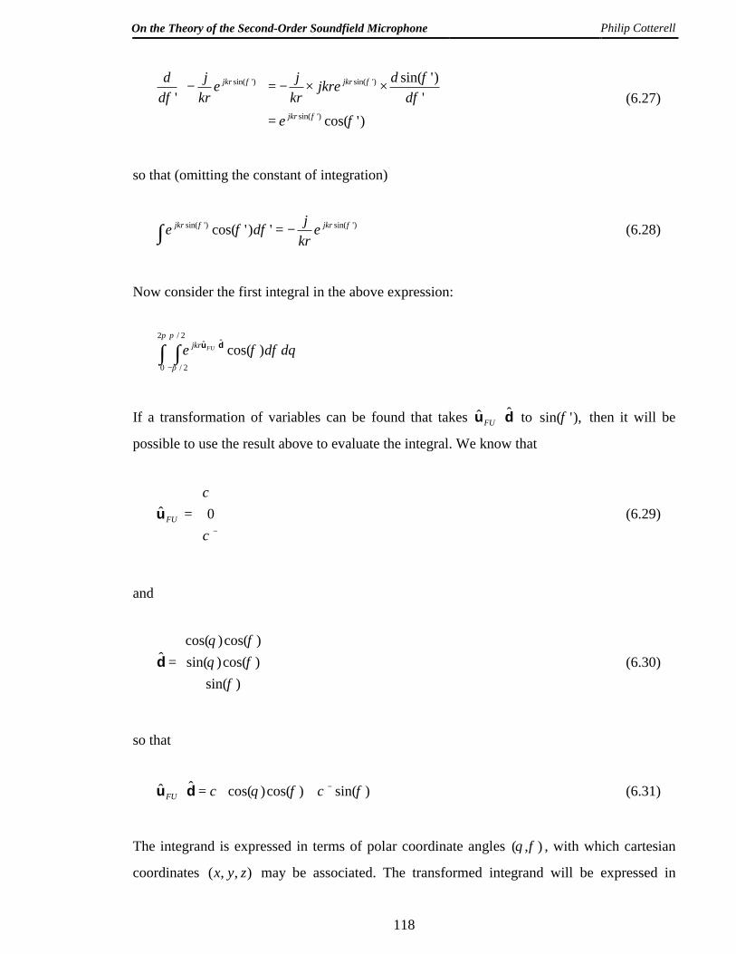
It is now necessary to evaluate each of the integrals in this expression. We first observe that
On the Theory of the Second-Order Soundfield Microphone Philip Cotterell
118
)'cos('
)'sin('
)'sin(
)'sin()'sin(
φ
φφ
φφ
φφ
jkr
jkrjkr
ed
djkrekrje
krj
dd
=
××−=
−
(6.27)
so that (omitting the constant of integration)
)'sin()'sin( ')'cos( φφ φφ jkrjkr ekrjde −=∫ (6.28)
Now consider the first integral in the above expression:
∫ ∫−
⋅π π
π
θφφ2
0
2/
2/
ˆˆ )cos( dde FUjkr du
If a transformation of variables can be found that takes du ˆˆ ⋅FU to ),'sin(φ then it will be
possible to use the result above to evaluate the integral. We know that
=−
+
χ
χ0ˆ FUu (6.29)
and
=
)sin()cos()sin()cos()cos(
ˆ
φφθφθ
d (6.30)
so that
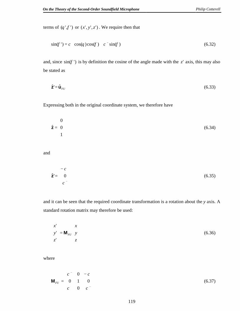
)sin()cos()cos(ˆˆ φχφθχ −+ +=⋅duFU (6.31)
The integrand is expressed in terms of polar coordinate angles ),( φθ , with which cartesian
coordinates ),,( zyx may be associated. The transformed integrand will be expressed in
On the Theory of the Second-Order Soundfield Microphone Philip Cotterell
119
terms of )','( φθ or )',','( zyx . We require then that
)sin()cos()cos()'sin( φχφθχφ −+ += (6.32)
and, since )'sin(φ is by definition the cosine of the angle made with the 'z axis, this may also
be stated as
FUuz ˆ'ˆ = (6.33)
Expressing both in the original coordinate system, we therefore have
=
100
z (6.34)
and
−=
−
+
χ
χ0'z (6.35)
and it can be seen that the required coordinate transformation is a rotation about the y axis. A
standard rotation matrix may therefore be used:
=
zyx
zyx
FUM'''
(6.36)
where
−=
−+
+−
χχ
χχ
0010
0
FUM (6.37)
On the Theory of the Second-Order Soundfield Microphone Philip Cotterell
120
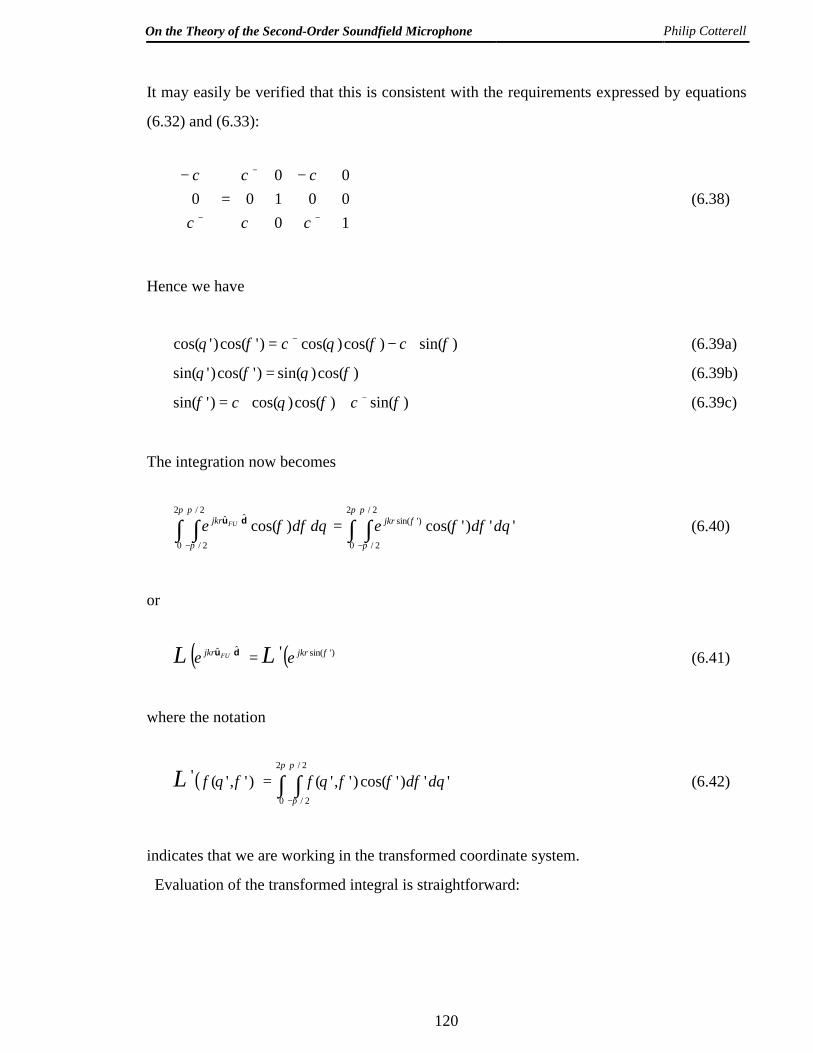
It may easily be verified that this is consistent with the requirements expressed by equations
(6.32) and (6.33):
−=
−
−+
+−
−
+
100
0010
00
χχ
χχ
χ
χ(6.38)
Hence we have
)sin()cos()cos()'cos()'cos( φχφθχφθ +− −= (6.39a)
)cos()sin()'cos()'sin( φθφθ = (6.39b)
)sin()cos()cos()'sin( φχφθχφ −+ += (6.39c)
The integration now becomes
∫ ∫∫ ∫−−
⋅ =π π
π
φπ π
π
θφφθφφ2
0
2/
2/
)'sin(2
0
2/
2/
ˆˆ '')'cos()cos( ddedde jkrjkr FU du (6.40)
or
( ) ( ))'sin(ˆˆ ' φΛΛ jkrjkr ee FU =⋅du (6.41)
where the notation
( ) ∫ ∫−
=π π
π
θφφφθφθΛ2
0
2/
2/
'')'cos()','()','(' ddff (6.42)
indicates that we are working in the transformed coordinate system.
Evaluation of the transformed integral is straightforward:
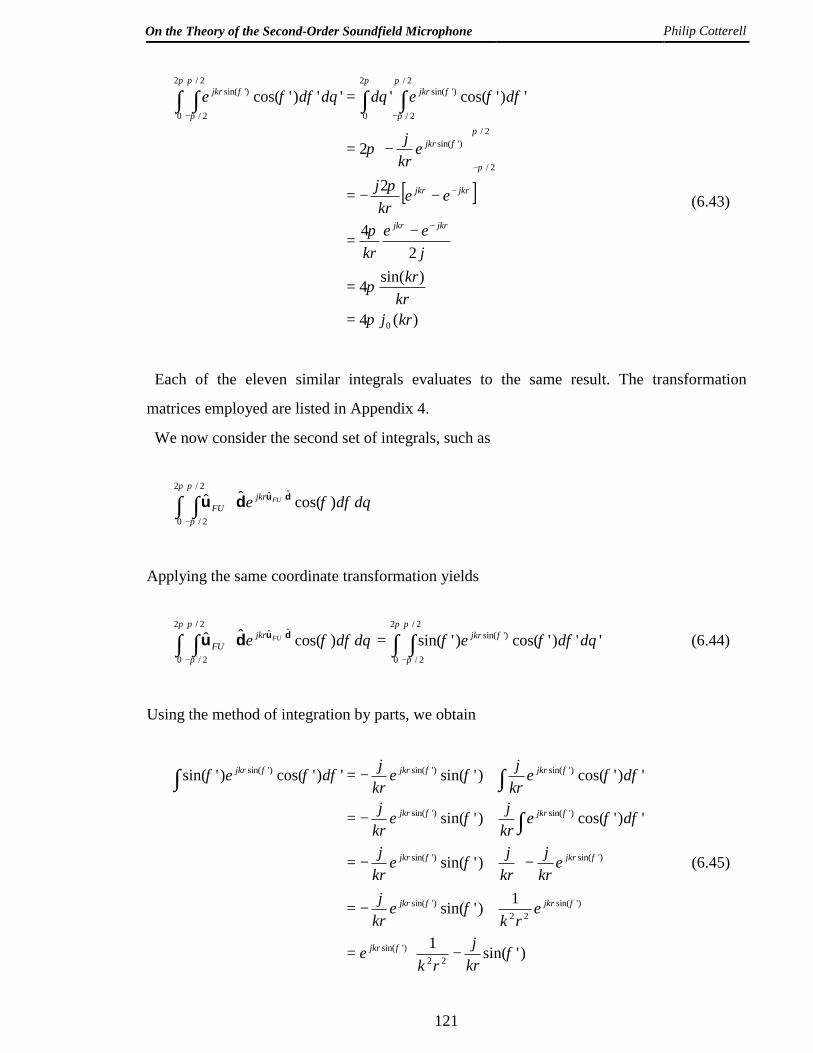
On the Theory of the Second-Order Soundfield Microphone Philip Cotterell
121
[ ]
)(4
)sin(4
24
2
2
')'cos(''')'cos(
0
2/
2/
)'sin(
2/
2/
)'sin(2
0
2
0
2/
2/
)'sin(
krjkr
krjee
kr
eekrj
ekrj
deddde
jkrjkr
jkrjkr
jkr
jkrjkr
π
π
π
π
π
φφθθφφ
π
π
φ
π
π
φππ π
π
φ
=
=
−=
−−=
−=
=
−
−
−
−−∫∫∫ ∫
(6.43)
Each of the eleven similar integrals evaluates to the same result. The transformation
matrices employed are listed in Appendix 4.
We now consider the second set of integrals, such as
∫ ∫−
⋅⋅π π
π
θφφ2
0
2/
2/
ˆˆ )cos(ˆˆ dde FUjkrFU
dudu
Applying the same coordinate transformation yields
∫ ∫∫ ∫−−
⋅ =⋅π π
π
φπ π
π
θφφφθφφ2
0
2/
2/
)'sin(2
0
2/
2/
ˆˆ '')'cos()'sin()cos(ˆˆ ddedde jkrjkrFU
FU dudu (6.44)
Using the method of integration by parts, we obtain
−=
+−=
−+−=
+−=
+−=
∫
∫∫
)'sin(1
1)'sin(
)'sin(
')'cos()'sin(
')'cos()'sin(')'cos()'sin(
22)'sin(
)'sin(22
)'sin(
)'sin()'sin(
)'sin()'sin(
)'sin()'sin()'sin(
φ
φ
φ
φφφ
φφφφφφ
φ
φφ
φφ
φφ
φφφ
krj
rke
erk
ekrj
ekrj
krje
krj
dekrje
krj
dekrje
krjde
jkr
jkrjkr
jkrjkr
jkrjkr
jkrjkrjkr
(6.45)
On the Theory of the Second-Order Soundfield Microphone Philip Cotterell
122
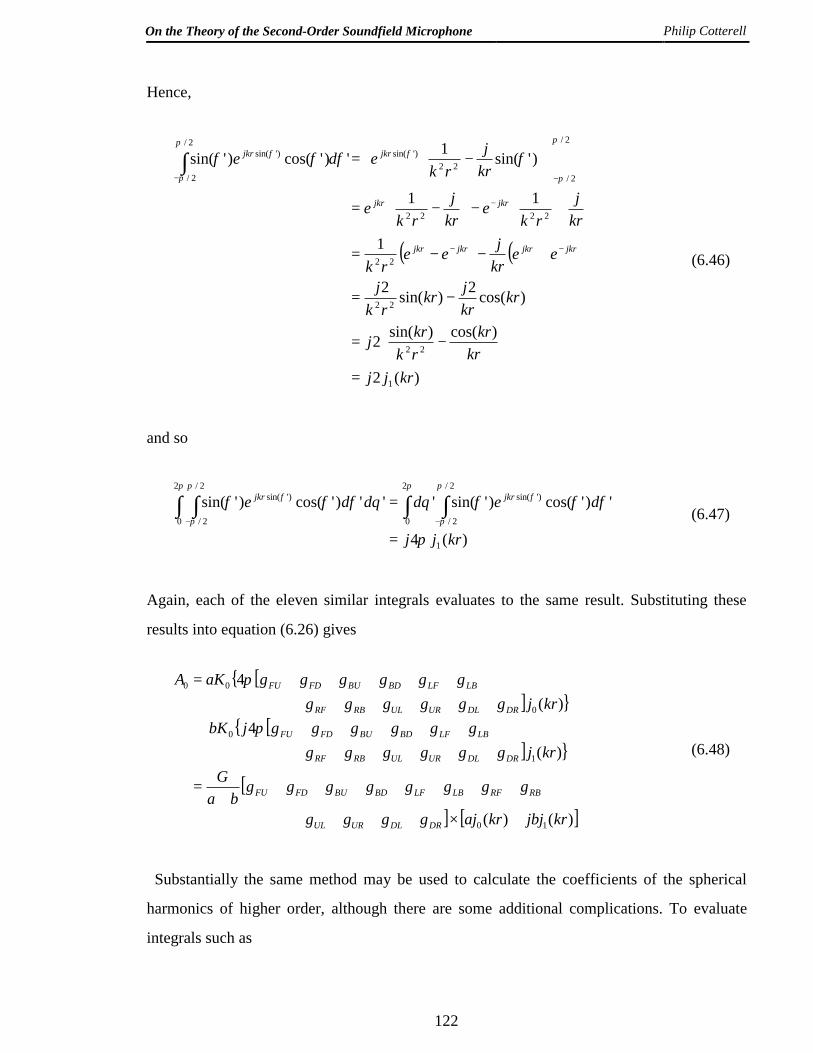
Hence,
( ) ( )
)(2
)cos()sin(2
)cos(2)sin(2
1
11
)'sin(1')'cos()'sin(
1
22
22
22
2222
2/
2/22
)'sin(2/
2/
)'sin(
krjjkr
krrkkrj
krkrjkr
rkj
eekrjee
rk
krj
rke
krj
rke
krj
rkede
jkrjkrjkrjkr
jkrjkr
jkrjkr
=
−=
−=
+−−=
+−
−=
−=
−−
−
−−∫
π
π
φπ
π
φ φφφφ
(6.46)
and so
)(4
')'cos()'sin(''')'cos()'sin(
1
2/
2/
)'sin(2
0
2
0
2/
2/
)'sin(
krjj
deddde jkrjkr
π
φφφθθφφφπ
π
φππ π
π
φ
=
= ∫∫∫ ∫−− (6.47)
Again, each of the eleven similar integrals evaluates to the same result. Substituting these
results into equation (6.26) gives
[{] }
[{] }
[] [ ])()(
)(4
)(4
10
1
0
0
00
krjbjkrajgggg
ggggggggba
Gkrjgggggg
ggggggjbKkrjgggggg
ggggggaKA
DRDLURUL
RBRFLBLFBDBUFDFU
DRDLURULRBRF
LBLFBDBUFDFU
DRDLURULRBRF
LBLFBDBUFDFU
+×++++
++++++++
=
++++++++++++
+++++++++++=
π
π
(6.48)
Substantially the same method may be used to calculate the coefficients of the spherical
harmonics of higher order, although there are some additional complications. To evaluate
integrals such as
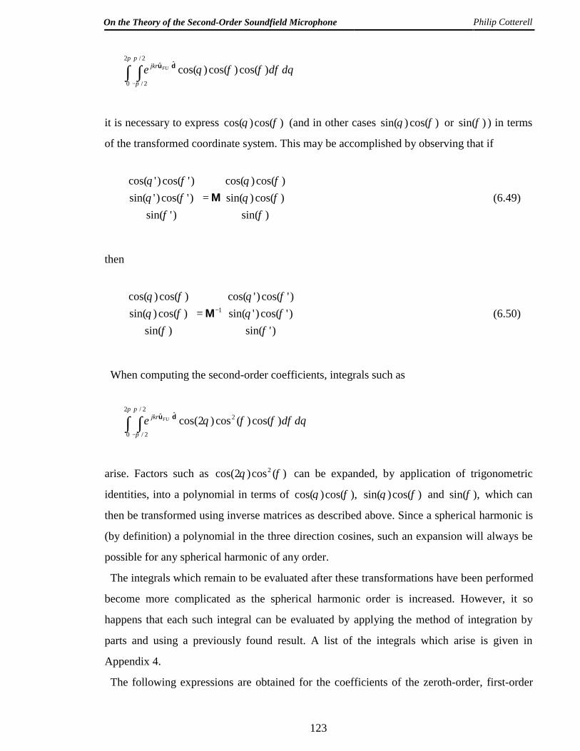
On the Theory of the Second-Order Soundfield Microphone Philip Cotterell
123
∫ ∫−
⋅π π
π
θφφφθ2
0
2/
2/
ˆˆ )cos()cos()cos( dde FUjkr du
it is necessary to express )cos()cos( φθ (and in other cases )cos()sin( φθ or )sin(φ ) in terms
of the transformed coordinate system. This may be accomplished by observing that if
=
)sin()cos()sin()cos()cos(
)'sin()'cos()'sin()'cos()'cos(
φφθφθ
φφθφθ
M (6.49)
then
=
−
)'sin()'cos()'sin()'cos()'cos(
)sin()cos()sin()cos()cos(
1
φφθφθ
φφθφθ
M (6.50)
When computing the second-order coefficients, integrals such as
∫ ∫−
⋅π π
π
θφφφθ2
0
2/
2/
2ˆˆ )cos()(cos)2cos( dde FUjkr du
arise. Factors such as )(cos)2cos( 2 φθ can be expanded, by application of trigonometric
identities, into a polynomial in terms of ),cos()cos( φθ )cos()sin( φθ and ),sin(φ which can
then be transformed using inverse matrices as described above. Since a spherical harmonic is
(by definition) a polynomial in the three direction cosines, such an expansion will always be
possible for any spherical harmonic of any order.
The integrals which remain to be evaluated after these transformations have been performed
become more complicated as the spherical harmonic order is increased. However, it so
happens that each such integral can be evaluated by applying the method of integration by
parts and using a previously found result. A list of the integrals which arise is given in
Appendix 4.
The following expressions are obtained for the coefficients of the zeroth-order, first-order
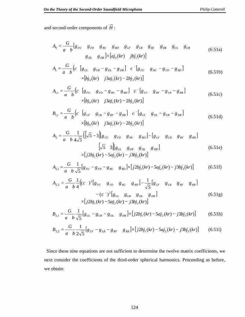
On the Theory of the Second-Order Soundfield Microphone Philip Cotterell
124
and second-order components of :~H
[] [ ])()( 10
0
krjbjkrajgg
ggggggggggba
GA
DRDL
URULRBRFLBLFBDBUFDFU
+×++
++++++++++
= (6.51a)
[ ] [ ]( )[ ])(2)(3)( 210
1
krbjkrajjkrbj
ggggggggba
GA BDFDBUFUDRDLURUL
−+×
−−++−−++
= −+ χχ(6.51b)
[ ] [ ]( )[ ])(2)(3)( 210
1,1
krbjkrajjkrbj
ggggggggba
GA RBLBRFLFBDBUFDFU
−+×
−−++−−++
= −+ χχ(6.51c)
[ ] [ ]( )[ ])(2)(3)( 210
1,1
krbjkrajjkrbj
ggggggggba
GB DRURDLULRBRFLBLF
−+×
−−++−−++
= −+ χχ(6.51d)
[ ][ ] [ ]([ ][ ])
[ ])(3)(5)(235
3554
1
321
2
krbjjkrajkrbjjgggg
ggggggggba
GA
DRDLURUL
RBRFLBLFBDBUFDFU
−−×+++++
+++−+++−+
=
(6.51e)
[ ] [ ])(3)(5)(25
13211,2 krbjjkrajkrbjjgggg
baGA BDBUFDFU −−×+−−+
= (6.51f)
[ ]( [ ]
[ ])[ ])(3)(5)(2
)(5
1)(41
321
2
22,2
krbjjkrajkrbjjgggg
ggggggggba
GA
DRDLURUL
RBRFLBLFBDBUFDFU
−−×+++−
+++−++++
=
−
+
χ
χ
(6.51g)
[ ] [ ])(3)(5)(25
13211,2 krbjjkrajkrbjjgggg
baGB DRDLURUL −−×+−−+
= (6.51h)
[ ] [ ])(3)(5)(252
13212,2 krbjjkrajkrbjjgggg
baGB RBRFLBLF −−×+−−+
= (6.51i)
Since these nine equations are not sufficient to determine the twelve matrix coefficients, we
next consider the coefficients of the third-order spherical harmonics. Proceeding as before,
we obtain:
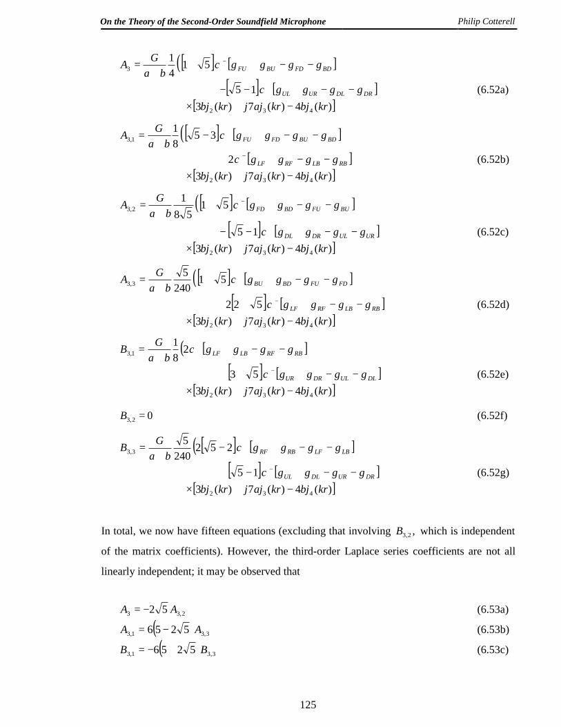
On the Theory of the Second-Order Soundfield Microphone Philip Cotterell
125
[ ] [ ]([ ] [ ])
[ ])(4)(7)(315
5141
432
3
krbjkrajjkrbjgggg
ggggba
GA
DRDLURUL
BDFDBUFU
−+×−−+−−
−−+++
=
+
−
χ
χ
(6.52a)
[ ] [ ]([ ])
[ ])(4)(7)(32
3581
432
1,3
krbjkrajjkrbjgggg
ggggba
GA
RBLBRFLF
BDBUFDFU
−+×−−++
−−+−+
=
−
+
χ
χ
(6.52b)
[ ] [ ]([ ] [ ])
[ ])(4)(7)(315
5158
1
432
2,3
krbjkrajjkrbjgggg
ggggba
GA
URULDRDL
BUFUBDFD
−+×−−+−−
−−+++
=
+
−
χ
χ
(6.52c)
[ ] [ ]([ ] [ ])
[ ])(4)(7)(3522
51240
5
432
3,3
krbjkrajjkrbjgggg
ggggba
GA
RBLBRFLF
FDFUBDBU
−+×−−+++
−−+++
=
−
+
χ
χ
(6.52d)
[ ]([ ] [ ])
[ ])(4)(7)(353
281
432
1,3
krbjkrajjkrbjgggg
ggggba
GB
DLULDRUR
RBRFLBLF
−+×−−+++
−−++
=
−
+
χ
χ
(6.52e)
02,3 =B (6.52f)
[ ] [ ]([ ] [ ])
[ ])(4)(7)(315
252240
5
432
3,3
krbjkrajjkrbjgggg
ggggba
GB
DRURDLUL
LBLFRBRF
−+×−−+−+
−−+−+
=
−
+
χ
χ
(6.52g)
In total, we now have fifteen equations (excluding that involving ,2,3B which is independent
of the matrix coefficients). However, the third-order Laplace series coefficients are not all
linearly independent; it may be observed that
2,33 52 AA −= (6.53a)
( ) 3,31,3 5256 AA −= (6.53b)
( ) 3,31,3 5256 BB +−= (6.53c)
On the Theory of the Second-Order Soundfield Microphone Philip Cotterell
126
Hence, we have obtained exactly twelve linearly independent equations in the twelve A-B
matrix coefficients; these can therefore now be determined. For each B-format signal, we set
the coefficient of the appropriate spherical harmonic to a suitable value, and all other
coefficients to zero; we then solve the resulting set of equations for the twelve matrix
coefficients. Note that, while this “suitable value” is 1 for the zeroth-order and first-order
component signals, it takes different values for the second-order signals because of the
scaling factors which appear in the definitions of the second-order spherical harmonics. For
example, the coefficient 2,2B is associated with the spherical harmonic );(cos)2sin(3 2 φθ
hence, to obtain the desired polar response, 2,2B must be set equal to .31
It is desired that the A-B matrix should be frequency-independent, as it is for the first-order
soundfield microphone; hence, the frequency response functions are omitted at this stage. For
convenience we also disregard the )( baG + factor. The A-B matrix derived therefore
depends only on the geometry of the array; the polar responses of the individual capsules will
be taken into account when designing the non-coincidence compensation filters.
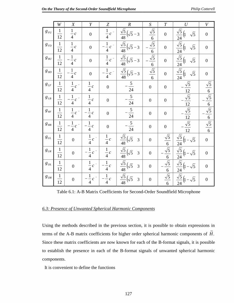
The matrix coefficients obtained are shown in table 6.1.
Note that each of the signals S, T and V is obtained from a rectangular arrangement of
capsules similar to that described in section 3.6.
On the Theory of the Second-Order Soundfield Microphone Philip Cotterell
127
W X Y Z R S T U VFUg
121 +χ
41
0 −χ41 ( )35
485
−65 0 ( )51
245
+ 0
FDg121 +χ
41
0 −− χ41 ( )35
485
−65
− 0 ( )5124
5+ 0
BUg121 +− χ
41
0 −χ41 ( )35
485
−65
− 0 ( )5124
5+ 0
BDg121 +− χ
41
0 −− χ41 ( )35
485
−65 0 ( )51
245
+ 0
LFg121 −χ
41 +χ
41
0 245
− 0 012
5−
65
LBg121 −− χ
41 +χ
41
0 245
− 0 012
5−
65
−
RFg121 −χ
41 +− χ
41
0 245
− 0 012
5−
65
−
RBg121 −− χ
41 +− χ
41
0 245
− 0 012
5−
65
ULg121
0 −χ41 +χ
41 ( )35
485
+ 065 ( )51
245
− 0
URg121
0 −− χ41 +χ
41 ( )35
485
+ 065
− ( )5124
5− 0
DLg121
0 −χ41 +− χ
41 ( )35
485
+ 065
− ( )5124
5− 0
DRg121
0 −− χ41 +− χ
41 ( )35
485
+ 065 ( )51
245
− 0
Table 6.1: A-B Matrix Coefficients for Second-Order Soundfield Microphone
6.3: Presence of Unwanted Spherical Harmonic Components
Using the methods described in the previous section, it is possible to obtain expressions in
terms of the A-B matrix coefficients for higher order spherical harmonic components of .~H
Since these matrix coefficients are now known for each of the B-format signals, it is possible
to establish the presence in each of the B-format signals of unwanted spherical harmonic
components.
It is convenient to define the functions
On the Theory of the Second-Order Soundfield Microphone Philip Cotterell
128
[ ]( )[ ]
−−+=
+−+−−=
−+−++−=
−
+−−
+−−
)()()1()12(
)()12()()1()()1(
)()1)(1()()12()()1(),(
11
11)1(
αναα
ν
ανααν
αναναναν
nnn
nnnn
nnnn
jd
djjnj
jnjnnjjjjnjnjjnjnИ
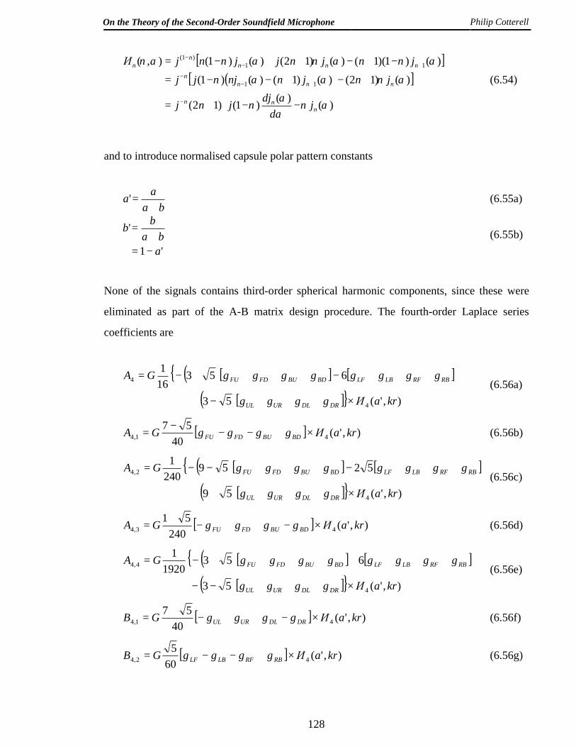
(6.54)
and to introduce normalised capsule polar pattern constants
baaa+
=' (6.55a)
'1
'
aba
bb
−=+
= (6.55b)
None of the signals contains third-order spherical harmonic components, since these were
eliminated as part of the A-B matrix design procedure. The fourth-order Laplace series
coefficients are
( )[ ]{ [ ]
( )[ ]} ),'(53
653161
4
4
kragggg
ggggggggGA
DRDLURUL
RBRFLBLFBDBUFDFU
И×+++−+
+++−++++−=(6.56a)
[ ] ),'(40
5741,4 kraggggGA BDBUFDFU И×+−−
−= (6.56b)
( )[ ] [ ]{( )[ ]} ),'(59
52592401
4
2,4
kragggg
ggggggggGA
DRDLURUL
RBRFLBLFBDBUFDFU
И×+++++
+++−+++−−=(6.56c)
[ ] ),'(240
5143,4 kraggggGA BDBUFDFU И×−++−
+= (6.56d)
( )[ ] [ ]{( )[ ]} ),'(53
6531920
1
4
4,4
kragggg
ggggggggGA
DRDLURUL
RBRFLBLFBDBUFDFU
И×+++−−
++++++++−=(6.56e)
[ ] ),'(40
5741,4 kraggggGB DRDLURUL И×−++−
+= (6.56f)
[ ] ),'(60
542,4 kraggggGB RBRFLBLF И×+−−= (6.56g)
On the Theory of the Second-Order Soundfield Microphone Philip Cotterell
129
[ ] ),'(240
1543,4 kraggggGB DRDLURUL И×+−−
−= (6.56h)
[ ] ),'(2401
44,4 kraggggGB RBRFLBLF И×+−−= (6.56i)
The fifth-order coefficients are given by
( ) [ ]{( ) [ ]} ),'(51135
51135400
5
5
5
kragggg
ggggGA
DRDLURUL
BDBUFDFU
И×++−−++
−+−−=
+
−
χ
χ(6.57a)
( ) [ ]{[ ]} ),'(510
5335400
5
5
1,5
kragggg
ggggGA
RBRFLBLF
BDBUFDFU
И×−+−+
++−−−=
−
+
χ
χ(6.57b)
( ) [ ]{( ) [ ]} ),'(15
15801
5
2,5
kragggg
ggggGA
DRDLURUL
BDBUFDFU
И×++−−++
+−+−−=
+
−
χ
χ(6.57c)
( ) [ ]{( ) [ ]} ),'(5252
5131920
1
5
3,5
kragggg
ggggGA
RBRFLBLF
BDBUFDFU
И×−+−++
−−+−=
−
+
χ
χ(6.57d)
( ) [ ]{( ) [ ]} ),'(53
531920
1
5
4,5
kragggg
ggggGA
DRDLURUL
BDBUFDFU
И×−−+−+
−+−+=
+
−
χ
χ(6.57e)
( ) [ ]{( ) [ ]} ),'(1522
5319200
1
5
5,5
kragggg
ggggGA
RBRFLBLF
BDBUFDFU
И×−+−−+
−−++=
−
+
χ
χ(6.57f)
[ ]{( ) [ ]} ),'(5335
510400
5
5
1,5
kragggg
ggggGB
DRDLURUL
RBRFLBLF
И×−+−++
−−+=
−
+
χ
χ(6.57g)
02,5 =B (6.57h)
( ) [ ]{( ) [ ]} ),'(513
25521920
1
5
3,5
kragggg
ggggGB
DRDLURUL
RBRFLBLF
И×+−+−++
++−−−=
−
+
χ
χ(6.57i)
04,5 =B (6.57j)
On the Theory of the Second-Order Soundfield Microphone Philip Cotterell
130
( ) [ ]{( ) [ ]} ),'(53
152219200
1
5
5,5
kragggg
ggggGB
DRDLURUL
RBRFLBLF
И×−+−−+
++−−+=
−
+
χ
χ(6.57k)
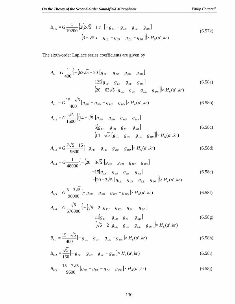
The sixth-order Laplace series coefficients are given by
( )[ ]{[ ]
( )[ ]} ),'(56320
125
205634001
6
6
kragggg
gggg
ggggGA
DRDLURUL
RBRFLBLF
BDBUFDFU
И×+++++
++++
+++−−=
(6.58a)
[ ] ),'(400
51561,6 kraggggGA BDBUFDFU И×+−−
+= (6.58b)
( )[ ]{[ ]
( )[ ]} ),'(514
5
5141600
5
6
2,6
kragggg
gggg
ggggGA
DRDLURUL
RBRFLBLF
BDBUFDFU
И×+++++
++++
+++−=
(6.58c)
[ ] ),'(9600
155763,6 kraggggGA BDBUFDFU И×−++−
−= (6.58d)
( )[ ]{[ ]
( )[ ]} ),'(5320
15
532048000
1
6
4,6
kragggg
gggg
ggggGA
DRDLURUL
RBRFLBLF
BDBUFDFU
И×+++−−
+++−
++++−=
(6.58e)
[ ] ),'(96000
53565,6 kraggggGA BDBUFDFU И×−++−
+= (6.58f)
( )[ ]{[ ]
( )[ ]} ),'(25
11
25576000
5
6
6,6
kragggg
gggg
ggggGA
DRDLURUL
RBRFLBLF
BDBUFDFU
И×+++−+
+++−
++++−=
(6.58g)
[ ] ),'(400
51561,6 kraggggB DRDLURUL И×−++−
−= (6.58h)
[ ] ),'(160
562,6 kraggggB RBRFLBLF И×−++−= (6.58i)
[ ] ),'(9600
571563,6 kraggggB DRDLURUL И×+−−
+= (6.58j)
On the Theory of the Second-Order Soundfield Microphone Philip Cotterell
131
[ ] ),'(2400
164,6 kraggggB RBRFLBLF И×−++−= (6.58k)
[ ] ),'(96000
55365,6 kraggggB DRDLURUL И×−++−
−= (6.58l)
[ ] ),'(288000
566,6 kraggggB RBRFLBLF И×+−−= (6.58m)
From these general expressions, the Laplace series coefficients for each of the B-format
signals are obtained by substituting in the known values for the A-B matrix coefficients. It so
happens that the majority of the coefficients in the Laplace series for each signal are zero;
only the non-zero coefficients are listed here.
For :~W
{ } ),'(8011~
66 kraWA GИ= (6.59a)
{ } ),'(1600
511~62,6 kraGWA И= (6.59b)
{ } ),'(28800
11~64,6 kraWA GИ−= (6.59c)
{ } ),'(115200
5~66,6 kraGWA И−= (6.59d)
For :~X
{ } ),'(400
15521~51,5 kraGXA И−
−= (6.60a)
{ } ),'(3200
5315~53,5 kraGXA И+
= (6.60b)
{ } ),'(19200
153~55,5 kraGXA И−
= (6.60c)
For :~Y
{ } ),'(400
15521~51,5 kraGYB И+
= (6.61a)
On the Theory of the Second-Order Soundfield Microphone Philip Cotterell
132
{ } ),'(3200
5315~53,5 kraGYB И−
−= (6.61b)
{ } ),'(19200
153~55,5 kraGYB И+
−= (6.61c)
For :~Z
{ } ),'(409~
55 kraGZA И−= (6.62a)
{ } ),'(200
53~52,5 kraGZA И−= (6.62b)
{ } ),'(9601~
54,5 kraGZA И= (6.62c)
For :~R
{ } ),'(165~
44 kraGRA И−= (6.63a)
{ } ),'(240
57~42,4 kraGRA И= (6.63b)
{ } ),'(3841~
44,4 kraGRA И−= (6.63c)
{ } ),'(12021~
66 kraRA GИ= (6.63d)
{ } ),'(480
53~62,6 kraRA GИ= (6.63e)
{ } ),'(14400
1~64,6 kraRA GИ= (6.63f)
{ } ),'(57600
5~66,6 kraRA GИ= (6.63g)
For :~S
{ } ),'(60
557~41,4 kraGSA И−
= (6.64a)
{ } ),'(360
55~43,4 kraGSA И+
−= (6.64b)
{ } ),'(120
153~61,6 kraSA GИ+
= (6.64c)
On the Theory of the Second-Order Soundfield Microphone Philip Cotterell
133
{ } ),'(2880
537~63,6 kraSA GИ−
−= (6.64d)
{ } ),'(28800
53~65,6 kraSA GИ+
−= (6.64e)
For :~T
{ } ),'(60
557~41,4 kraGTB И+
−= (6.65a)
{ } ),'(360
55~43,4 kraGTB И−
= (6.65b)
{ } ),'(120
153~61,6 kraTB GИ−
−= (6.65c)
{ } ),'(2880
537~63,6 kraTB GИ+
= (6.65d)
{ } ),'(28800
53~65,6 kraTB GИ−
−= (6.65e)
For :~U
{ } ),'(24
57~44 kraGUA И= (6.66a)
{ } ),'(241~
42,4 kraGUA И−= (6.66b)
{ } ),'(2880
57~44,4 kraGUA И−= (6.66c)
{ } ),'(20
57~66 kraUA GИ−= (6.66d)
{ } ),'(2401~
62,6 kraUA GИ= (6.66e)
{ } ),'(7200
5~64,6 kraUA GИ−= (6.66f)
{ } ),'(86400
1~66,6 kraUA GИ= (6.66g)
On the Theory of the Second-Order Soundfield Microphone Philip Cotterell
134
For :~V
{ } ),'(181~
42,4 kraGVB И= (6.67a)
{ } ),'(360
5~44,4 kraGVB И= (6.67b)
{ } ),'(481~
62,6 kraVB GИ−= (6.67c)
{ } ),'(3600
5~64,6 kraVB GИ−= (6.67d)
{ } ),'(86400
1~66,6 kraVB GИ= (6.67e)
From these results it can be seen that W~ is corrupted by unwanted spherical harmonics of
order six; the first-order component signals are corrupted by spurious fifth-order spherical
harmonics; and the second-order signals contain both fourth-order and sixth-order unwanted
spherical harmonic components.
In Chapter 5, it was noted that the B-format signals obtained from the first-order soundfield
microphone are contaminated by spurious second-order or third-order spherical harmonics.
The second-order soundfield microphone therefore represents a considerable improvement in
this respect. Since the higher order spherical harmonics have coefficients which depend on
higher order spherical Bessel functions, which in turn remain small up until greater values of
kr, so it may be expected that the maximum frequency to which effective coincidence is
maintained will exceed that given by equation (5.9). This advantage will, however, probably
be opposed to some extent by the fact that the array radius is likely to larger for a second-
order soundfield microphone.
6.4: Non-Coincidence Compensation Filtering
The author has not considered the design of non-coincidence compensation filters in detail;
the design of practical approximations to the theoretically ideal characteristics is a matter of
practical implementation rather than fundamental theory, and therefore outside the scope of
this thesis. Nevertheless, the following observations can be made.
By substituting the coefficients given in table 6.1 into equation (6.51), we obtain the
On the Theory of the Second-Order Soundfield Microphone Philip Cotterell
135
following results:
{ } [ ])(')('~100 krjjbkrjaGWA += (6.68a)
{ } [ ]),'(
)('2)('3)('~
1
2101
kraGИkrjbkrjajkrjbGZA
=−+=
(6.68b)
{ } [ ]),'(
)('2)('3)('~
1
2101,1
kraGИkrjbkrjajkrjbGXA
=
−+=(6.68c)
{ } [ ]),'(
)('2)('3)('~
1
2101,1
kraGИkrjbkrjajkrjbGYB
=
−+=(6.68d)
{ } [ ]),'(
)('3)('5)('2~
2
3212
kraGИkrjbjkrjakrjbjGRA
−=−−=
(6.68e)
{ } [ ]
),'(32
)('3)('5)('232~
2
3211,2
kraИG
krjbjkrjakrjbjGSA
−=
−−=(6.68f)
{ } [ ]
),'(31
)('3)('5)('231~
2
3212,2
kraИG
krjbjkrjakrjbjGUA
−=
−−=(6.68g)
{ } [ ]
),'(32
)('3)('5)('232~
2
3211,2
kraИG
krjbjkrjakrjbjGTB
−=
−−=(6.68h)
{ } [ ]
),'(31
)('3)('5)('231~
2
3212,2
kraИG
krjbjkrjakrjbjGVB
−=
−−=(6.68i)
The factors of 32 and 3
1 in the expressions for ,1,2A ,2,2A ,1,2B and 2,2B are due to the
factors of 23 and 3 which appear in the definitions of the corresponding spherical harmonics
(see page 128); they therefore do not imply the need for compensatory scaling of the signals.
The impulse responses corresponding to these frequency response functions may be found
by taking the inverse Fourier transforms. Let
cr
=τ (6.69)
On the Theory of the Second-Order Soundfield Microphone Philip Cotterell
136
then
τω=rk (6.70)
and employing the inverse Fourier transforms of the spherical Bessel functions developed in
Chapter 2, we obtain
[ ]{ }
( ) )(''2
)(')('ˆ)(
2
101
0
tratbGjjbjaGFt
τττ
τωτω∆
+−=
+= −
(6.71a)
{ }
( ) )(''23
),'(ˆ)(
23
11
1
trtatbGaGИFt
τττ
τω∆
−=
= −
(6.71b)
{ }
( ) )('''3'345
),'(ˆ)(
32234
21
2
tratbtatbGaGИFt
τττττ
τω∆
−++−=
−= −
(6.71c)
where
<<−
=otherwise0
1)(
τττ
ttr (6.72)
It may be noted that the frequency responses of the desired spherical harmonic components
of the zeroth-order and first-order signals have the same form as in the case of the first-order
soundfield microphone. Filters that have proved to give acceptable results with the first-order
soundfield microphone might well therefore be equally suitable for use with the second-order
microphone.
In the case of the second-order signals, the required filtering is fundamentally different in
one respect. From equation (2.14), it can be seen that the frequency response function for the
second-order spherical harmonic components becomes zero for .0=kr This is because we
are approximating second-order directional derivatives by taking the difference between the
outputs of first-order microphone capsules. An integration with respect to time is therefore
necessary, not to compensate for the spacing of the capsules, but as a fundamental part of the
On the Theory of the Second-Order Soundfield Microphone Philip Cotterell
137
method being utilised to obtain the signals. The filtering will therefore serve a dual purpose
so far as these signals are concerned, since at higher frequencies compensation for the effects
of the capsule spacing will still be required.
It must be noted that suitable filters cannot be designed on the basis of theory alone. During
the development of the first-order soundfield microphone, it was found that although filters
developed from theoretical analysis gave a substantial improvement over arrays without
filtering, to obtain optimum performance it was necessary to take into account experimental
information [7]. Certainly one expects that this will be the case with the second-order
soundfield microphone as well, since there will inevitably be departures from ideal behaviour
which are not represented in the theoretical treatment.
6.5: Additional B-Format Signal Processing
6.5.1: Rotation & Elevation
The rotation and elevation controls for the second-order soundfield microphone must clearly
have an identical effect on the zeroth-order and first-order signals as in the case of the first-
order microphone.
By trigonometric manipulation it may be established that the rotation control modifies the
second-order component signals as follows:
12 RR = (6.73a)
112 )sin()cos( TSS θθ += (6.73b)
112 )cos()sin( TST θθ +−= (6.73c)
112 )2sin()2cos( VUU θθ += (6.73d)
112 )2cos()2sin( VUV θθ +−= (6.73e)
The effect of the elevation control on the second-order signals may similarly be established to
be:
( ) ( ) 183
143
141
2 )2cos(1)2sin()2cos(31 USRR φφφ −+−+= (6.74a)
On the Theory of the Second-Order Soundfield Microphone Philip Cotterell
138
121
112 )2sin()2cos()2sin( USRS φφφ −+= (6.74b)
112 )sin()cos( VTT φφ −= (6.74c)
( ) ( ) 141
121
121
2 )2cos(3)2sin()2cos(1 USRU φφφ +++−= (6.74d)
112 )cos()sin( VTV φφ += (6.74e)
6.5.2: Side-Fire / End-Fire Switching & Inversion
The compensatory signal processing required to facilitate end-fire operation is:
12 WW = (6.75a)
12 ZX = (6.75b)
12 YY = (6.75c)
12 XZ −= (6.75d)
143
121
2 URR +−= (6.75e)
12 SS −= (6.75f)
12 VT = (6.75g)
121
12 URU += (6.75h)
12 TV = (6.75i)
As in the case of the first-order soundfield microphone, inverted operation requires only a
polarity reversal of some of the B-format signals:
12 YY −= (6.76a)
12 ZZ −= (6.76b)
12 SS −= (6.76c)
12 TT −= (6.76d)
12 VV −= (6.76e)
6.5.3: Dominance
The author has proved that it is not possible to extend the dominance transformation to work
On the Theory of the Second-Order Soundfield Microphone Philip Cotterell
139
with the second-order B-format signal set.
Suppose that the transformation can be extended to accommodate the second-order
component signals. The transformed signals must be linear combinations of the existing
signals; hence, there must exist coefficients ,'W ,'X ,'Y 'U and ,'V presumably functions
of λ, such that
)2sin(')2cos(')sin(')cos('')2cos( 11111111122 θθθθθ AVAUAYAXAWA ++++= (6.77)
Note that it is sufficient to consider only the pantophonic case, since the periphonic case
essentially reduces to this for .0=φ Complications due to the non-zero response of R for
directions in the horizontal plane are avoided by using a notional signal which encodes only
amplitude; whether this notional signal is in actuality proportional to W or to a combination
of W and R is unimportant. The 21 scaling of W is also neglected for convenience.
We know that
( ) ( )[ ] 111
12 )cos(1)cos(121 AA θλθλ −++= − (6.78a)
( )( ) )cos(11
)cos(11)cos(1
221
22
2 θλλθλλ
θ−++++−
= (6.78b)
( ) )cos(11)sin(2
)sin(1
221
2 θλλθλ
θ−++
= (6.78c)
and also that )2cos( 22 θA can be found by using the identity
)(sin)(cos)2cos( 22 θθθ −= (6.79)
By taking various values of θ, it is possible to generate a set of simultaneous equations which
can then be solved for ,'W ,'X etc.
i) Let .01 =θ Then
12 AA λ= (6.80a)
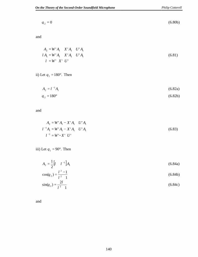
On the Theory of the Second-Order Soundfield Microphone Philip Cotterell
140
02 =θ (6.80b)
and
'''''''''
1111
1112
UXWAUAXAWAAUAXAWA
++=++=++=
λλ (6.81)
ii) Let .1801 °=θ Then
11
2 AA −= λ (6.82a)
°= 1802θ (6.82b)
and
''''''
'''
11111
11112
UXWAUAXAWAAUAXAWA
+−=
+−=
+−=
−
−
λ
λ (6.83)
iii) Let .901 °=θ Then
[ ] 11
2 21 AA −+= λλ (6.84a)
11)cos( 2
2
2 +−
=λλ
θ (6.84b)
12)sin( 22 +
=λ
λθ (6.84c)
and
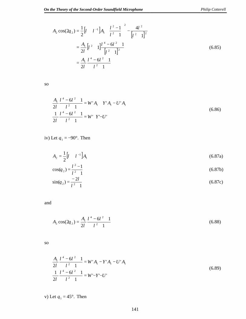
On the Theory of the Second-Order Soundfield Microphone Philip Cotterell
141
[ ] [ ][ ] [ ]
116
2
1161
2
14
11
21)2cos(
2
241
22
2421
22
22
2
2
11
22
++−
=
+
+−+=
+−
+−
+= −
λλλ
λ
λ
λλλ
λ
λ
λλλ
λλθ
A
A
AA
(6.85)
so
'''1
1621
'''1
162
2
24
1112
241
UYW
AUAYAWA
−+=+
+−
−+=+
+−
λλλ
λ
λλλ
λ (6.86)
iv) Let .901 °−=θ Then
[ ] 11
2 21 AA −+= λλ (6.87a)
11)cos( 2
2
2 +−
=λλ
θ (6.87b)
12)sin( 22 +
−=
λλ
θ (6.87c)
and
116
2)2cos( 2
241
22 ++−
=λ
λλλ
θAA (6.88)
so
'''1
1621
'''1
162
2
24
1112
241
UYW
AUAYAWA
−−=+
+−
−−=+
+−
λλλ
λ
λλλ
λ (6.89)
v) Let .451 °=θ Then
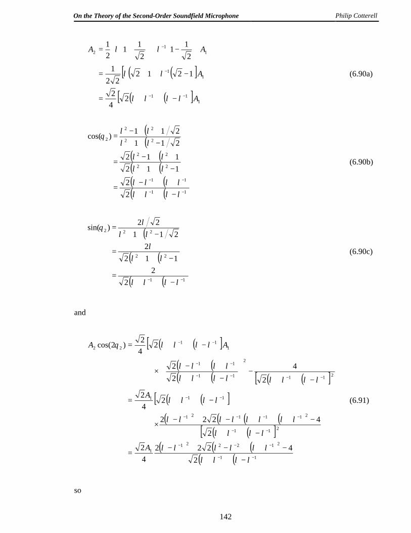
On the Theory of the Second-Order Soundfield Microphone Philip Cotterell
142
( ) ( )[ ]
( ) ( )[ ] 111
11
11
2
242
121222
12
112
1121
A
A
AA
−−
−
−
−++=
−++=
−+
+=
λλλλ
λλ
λλ
(6.90a)
( )( )
( ) ( )( ) ( )( ) ( )( ) ( )11
11
22
22
22
22
2
22
112112
211211)cos(
−−
−−
−++++−
=
−++++−
=
−++++−
=
λλλλλλλλ
λλλλ
λλλλ
θ
(6.90b)
( )
( ) ( )
( ) ( )11
22
222
22
1122
21122)sin(
−− −++=
−++=
−++=
λλλλ
λλλ
λλλ
θ
(6.90c)
and
( ) ( )[ ]( ) ( )( ) ( ) ( ) ( )[ ]
( ) ( )[ ]( ) ( )( ) ( )
( ) ( )[ ]( ) ( ) ( )
( ) ( )11
2122211
211
211121
111
211
2
11
11
111
22
24222
42
2
4222
242
2
422
242)2cos(
−−
−−−
−−
−−−−
−−
−−−−
−−
−−
−++−++−+−
=
−++
−+++−+−×
−++=
−++−
−++++−
×
−++=
λλλλλλλλλλ
λλλλ
λλλλλλλλ
λλλλ
λλλλλλλλλλλλ
λλλλθ
A
A
AA
(6.91)
so
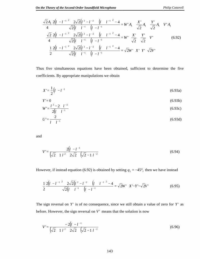
On the Theory of the Second-Order Soundfield Microphone Philip Cotterell
143
( ) ( ) ( )( ) ( )
( ) ( ) ( )( ) ( )
( ) ( ) ( )( ) ( ) '2'''2
24222
21
'2'
2''
24222
42
'2'
2''
24222
42
11
212221
11
212221
111111
2122211
VYXW
VYXW
AVAYAXAWA
+++=−++
−++−+−
+++=−++
−++−+−
+++=−++
−++−+−
−−
−−−
−−
−−−
−−
−−−
λλλλλλλλλλ
λλλλλλλλλλ
λλλλλλλλλλ
(6.92)
Thus five simultaneous equations have been obtained, sufficient to determine the five
coefficients. By appropriate manipulations we obtain
( )1
21' −−= λλX (6.93a)
0'=Y (6.93b)
( )1
22
22' −
−
++−
=λλ
λλW (6.93c)
1
2' −+=
λλU (6.93d)
and
( )( ) ( ) 22
1
1222122'
−
−
−+++−
=λλ
λλV (6.94)
However, if instead equation (6.92) is obtained by setting ,451 °−=θ then we have instead
( ) ( ) ( )( ) ( ) '2'''2
24222
21
11
212221
VYXW −−+=−++
−++−+−−−
−−−
λλλλλλλλλλ (6.95)
The sign reversal on 'Y is of no consequence, since we still obtain a value of zero for 'Y as
before. However, the sign reversal on 'V means that the solution is now
( )( ) ( ) 22
1
1222122'
−
−
−+++−−
=λλ
λλV (6.96)
On the Theory of the Second-Order Soundfield Microphone Philip Cotterell
144
We have thus obtained a contradiction, since equations (6.94) and (6.96) cannot
simultaneously be satisfied. Hence, it is not possible to find coefficients ,'W ,'X etc.,
independent of θ, such that equation (6.77) is satisfied, and so it is not possible to extend the
dominance transformation to the second-order case.