696 IEEE TRANSACTIONS ON ROBOTICS, VOL. 27, NO. 4, AUGUST

696 IEEE TRANSACTIONS ON ROBOTICS, VOL. 27, NO. 4, AUGUST 2011

The Hybrid Reciprocal Velocity ObstacleJamie Snape, Student Member, IEEE, Jur van den Berg, Stephen J. Guy, and Dinesh Manocha

Abstract—We present the hybrid reciprocal velocity obstaclefor collision-free and oscillation-free navigation of multiple mo-bile robots or virtual agents. Each robot senses its surroundingsand acts independently without central coordination or commu-nication with other robots. Our approach uses both the currentposition and the velocity of other robots to compute their futuretrajectories in order to avoid collisions. Moreover, our approach isreciprocal and avoids oscillations by explicitly taking into accountthat the other robots sense their surroundings as well and changetheir trajectories accordingly. We apply hybrid reciprocal velocityobstacles to iRobot Create mobile robots and demonstrate direct,collision-free, and oscillation-free navigation.

Index Terms—Collision avoidance, mobile robots, motion plan-ning, multirobot systems, navigation.

I. INTRODUCTION

MANY recent works have considered the problem of nav-igating a robot in an environment composed of dynamic

obstacles [1]–[5]. Some of the simplest approaches predictwhere the dynamic obstacles may be in the future by extrap-olating their current velocities, and let the robot avoid collisionsaccordingly. However, such techniques are not sufficient when arobot encounters other robots, because treating the other robotsas dynamic obstacles overlooks the reciprocity between robots.In other words, the other robots are not passive but are activelytrying to avoid collisions. Therefore, the future trajectories ofother robots cannot be estimated by simply extrapolating theircurrent velocities, since this would inherently cause undesirableoscillations in their trajectories [6].

In this paper, we present the hybrid reciprocal velocity ob-stacle for navigation of multiple mobile robots or virtual agentsthat explicitly considers the reciprocity between robots. Infor-mally, reciprocity lets a robot take half of the responsibility foravoidance of collisions with another robot and assumes that theother robot takes the other half. In a multirobot environment, thisconcept extends to every pair of robots. Each robot executes anindependent feedback loop, in which it chooses its new velocity

Manuscript received August 23, 2010; revised January 13, 2011; acceptedFebruary 21, 2011. Date of publication April 7, 2011; date of current versionAugust 10, 2011. This paper was recommended for publication by AssociateEditor S. Carpin and Editor J.-P. Laumond upon evaluation of the reviewers’comments. This work was supported by the Army Research Office under Con-tract W911NF-04-1-0088, by the National Science Foundation under Award0636208, Award 0917040, and Award 0904990, by the Defense AdvancedResearch Projects Agency and the U.S. Army Research, Development, andEngineering Command under Contract WR91CRB-08-C-0137, and by IntelCorporation. This paper was presented in part at the IEEE/RSJ InternationalConference on Intelligent Robots and Systems, St. Louis, MO, October 2009.

The authors are with the Department of Computer Science, Universityof North Carolina at Chapel Hill, Chapel Hill, NC 27599 USA (e-mail:[email protected]; [email protected]; [email protected]; [email protected]).

Color versions of one or more of the figures in this paper are available onlineat http://ieeexplore.ieee.org.

Digital Object Identifier 10.1109/TRO.2011.2120810

based on observations of the current positions and velocities ofthe other robots in close proximity. The robots do not communi-cate with each other but implicitly assume that the other robotsuse the same navigation strategy based on reciprocity. Our over-all approach can also deal with both static and dynamic obstaclesand incorporate a global navigation roadmap, if required.

The hybrid reciprocal velocity obstacle is an extension of thereciprocal velocity obstacle [6] that was introduced to addresssimilar issues in multiagent simulation. However, the reciprocalvelocity obstacle formulation has some limitations, particularlythat it frequently causes agents to end up in a “reciprocal dance”[7] as they cannot reach agreement on which side to pass eachother. To overcome this drawback, the hybrid reciprocal velocityobstacle enlarges the reciprocal velocity obstacle on the side thatthe robots should not pass. Consequently, if a robot attempts topass on the wrong side of another robot, then the robot has togive full priority to the other robot. If the robot chooses thecorrect side, then it can assume the cooperation of the otherrobot and retains equal priority.

We have implemented and applied our approach to a set ofiRobot Create mobile robots moving in an indoor environmentusing centralized sensing from an overhead video camera andBluetooth wireless remote control. Our experiments show thatour approach achieves direct, collision-free, and oscillation-freenavigation in an environment containing multiple mobile robotsand dynamic obstacles, even with some uncertainty in positionand velocity. We also demonstrate the ability to handle staticobstacles and the low computational requirements and scalabil-ity of the hybrid reciprocal velocity obstacle in two simulationsof multiple virtual agents.

The rest of this paper is organized in the following man-ner. We begin by summarizing related prior work in Section II.We formally define the problem of navigating multiple mobilerobots in Section III. In Section IV, we introduce our formula-tion of hybrid reciprocal velocity obstacles. In Section V, weuse this formulation for navigation of multiple mobile robotsand take into account obstacles in the environment as well asuncertainty in radius, position, and velocity, and the dynamicsand kinematics of the robots. We discuss implementation andpresent experimental results in Section VI.

II. PRIOR WORK

In this section, we give a brief overview of prior work on localand reactive navigation and existing variations of the velocityobstacle concept.

A. Local and Reactive Navigation

Reactive navigation differs from traditional global path plan-ning approaches, for example [4], [8], and [9], in that rather than

1552-3098/$26.00 © 2011 IEEE

SNAPE et al.: HYBRID RECIPROCAL VELOCITY OBSTACLE 697

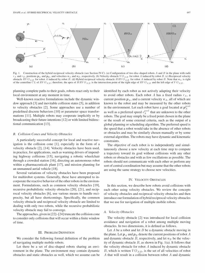
Fig. 1. Construction of the hybrid reciprocal velocity obstacle (see Section IV-C). (a) Configuration of two disc-shaped robots A and B in the plane with radiirA and rB , positions pA and pB , and velocities vA and vB , respectively. (b) Velocity obstacle V OA |B for robot A induced by robot B . (c) Reciprocal velocityobstacle RV OA |B for robot A induced by robot B . (d) Hybrid reciprocal velocity obstacle HRV OA |B for robot A induced by robot B . Note that vA is rightof the centerline CL of RV OA |B ; therefore, the apex of HRV OA |B is the intersection point of the right edge of RV OA |B and the left edge of V OA |B .

planning complete paths to their goals, robots react only to theirlocal environment at any moment in time.

Well-known reactive formulations include the dynamic win-dow approach [3] and inevitable collision states [5], in additionto velocity obstacles [2]. Some approaches use a number ofpredefined discrete behaviors [10] or parameter space transfor-mations [11]. Multiple robots may cooperate implicitly or bybroadcasting their future intentions [12] or with limited bidirec-tional communication [13].

B. Collision Cones and Velocity Obstacles

A particularly successful concept for local and reactive nav-igation is the collision cone [1], especially in the form of avelocity obstacle [2], [14]. Velocity obstacles have been used,in practice, for applications, such as warning drivers of impend-ing highway collisions [15], navigating a robotic wheelchairthrough a crowded station [16], directing an autonomous robotwithin a pharmaceuticals plant [17], and mission planning foran unmanned aerial vehicle [18].

Several variations of velocity obstacles have been proposedfor multirobot systems. Generally, these have attempted to in-corporate the reactive behavior of the other robots in the environ-ment. Formulations, such as common velocity obstacles [19],recursive probabilistic velocity obstacles [20], [21], and recip-rocal velocity obstacles [6], use various means to handle reci-procity, but all have shortcomings. Specifically, the commonvelocity obstacle and reciprocal velocity obstacle are limited todealing with only two robots, while the recursive probabilisticvelocity obstacle may fail to converge.

The approaches, given in [22]–[24] truncate the collision coneto consider only collisions that will occur within a finite windowof time.

III. PROBLEM DEFINITION

We consider the following formal definition of the problemof navigating multiple mobile robots.

Let there be a set of disc-shaped robots sharing an envi-ronment in the plane. The environment may contain dynamicobstacles and static obstacles as well, which we assume can be

identified by each robot as not actively adapting their velocityto avoid other robots. Each robot A has a fixed radius rA , acurrent position pA , and a current velocity vA , all of which areknown to the robot and may be measured by the other robotsin the environment. Let each robot have a goal located at pgoal

A

as well as a preferred speed vprefA that are unknown to the other

robots. The goal may simply be a fixed point chosen in the planeor the result of some external criteria, such as the output of aglobal planning or scheduling algorithm. The preferred speed isthe speed that a robot would take in the absence of other robotsor obstacles and may be similarly chosen manually or by someexternal algorithm. The robots may have dynamic and kinematicconstraints.

The objective of each robot is to independently and simul-taneously choose a new velocity at each time step to computea trajectory toward its goal without collisions with any otherrobots or obstacles and with as few oscillations as possible. Therobots should not communicate with each other or perform anysort of central coordination but may assume that the other robotsare using the same strategy to choose new velocities.

IV. VELOCITY OBSTACLES

In this section, we describe how robots avoid collisions witheach other using velocity obstacles. We review the conceptsof velocity obstacles and reciprocal velocity obstacles and thenintroduce our formulation of hybrid reciprocal velocity obstaclesthat we use for navigation of multiple mobile robots.

A. Velocity Obstacles

The velocity obstacle [2] was introduced for local collisionavoidance and navigation of a robot among multiple movingobstacles. In two dimensions, it is defined as follows.

Let A be a robot and let B be a dynamic obstacle moving inthe plane. Let pA and pB denote the current positions of robot Aand dynamic obstacle B, respectively, and let vB be the veloc-ity of dynamic obstacle B, as shown in Fig. 1(a). It follows thatthe velocity obstacle for robot A induced by dynamic obstacleB, which is written V OA |B , is the set of all velocities of robotA that will result in a collision between robot A and dynamic


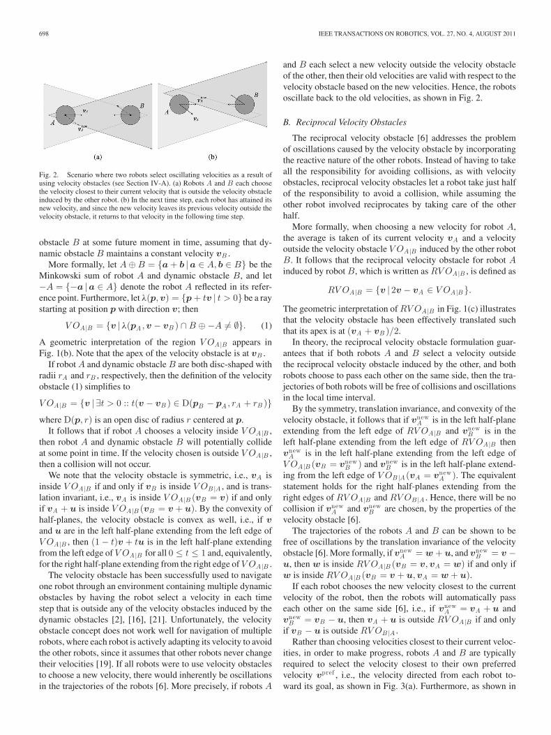
Fig. 2. Scenario where two robots select oscillating velocities as a result ofusing velocity obstacles (see Section IV-A). (a) Robots A and B each choosethe velocity closest to their current velocity that is outside the velocity obstacleinduced by the other robot. (b) In the next time step, each robot has attained itsnew velocity, and since the new velocity leaves its previous velocity outside thevelocity obstacle, it returns to that velocity in the following time step.

obstacle B at some future moment in time, assuming that dy-namic obstacle B maintains a constant velocity vB .

More formally, let A ⊕ B = {a + b |a ∈ A, b ∈ B} be theMinkowski sum of robot A and dynamic obstacle B, and let−A = {−a |a ∈ A} denote the robot A reflected in its refer-ence point. Furthermore, let λ(p,v) = {p + tv | t > 0} be a raystarting at position p with direction v; then

V OA |B = {v | λ(pA ,v − vB ) ∩ B ⊕−A �= ∅}. (1)

A geometric interpretation of the region V OA |B appears inFig. 1(b). Note that the apex of the velocity obstacle is at vB .

If robot A and dynamic obstacle B are both disc-shaped withradii rA and rB , respectively, then the definition of the velocityobstacle (1) simplifies to

V OA |B = {v | ∃t > 0 :: t(v − vB ) ∈ D(pB − pA , rA + rB )}where D(p, r) is an open disc of radius r centered at p.

It follows that if robot A chooses a velocity inside V OA |B ,then robot A and dynamic obstacle B will potentially collideat some point in time. If the velocity chosen is outside V OA |B ,then a collision will not occur.

We note that the velocity obstacle is symmetric, i.e., vA isinside V OA |B if and only if vB is inside V OB |A , and is trans-lation invariant, i.e., vA is inside V OA |B (vB = v) if and onlyif vA + u is inside V OA |B (vB = v + u). By the convexity ofhalf-planes, the velocity obstacle is convex as well, i.e., if vand u are in the left half-plane extending from the left edge ofV OA |B , then (1 − t)v + tu is in the left half-plane extendingfrom the left edge of V OA |B for all 0 ≤ t ≤ 1 and, equivalently,for the right half-plane extending from the right edge of V OA |B .

The velocity obstacle has been successfully used to navigateone robot through an environment containing multiple dynamicobstacles by having the robot select a velocity in each timestep that is outside any of the velocity obstacles induced by thedynamic obstacles [2], [16], [21]. Unfortunately, the velocityobstacle concept does not work well for navigation of multiplerobots, where each robot is actively adapting its velocity to avoidthe other robots, since it assumes that other robots never changetheir velocities [19]. If all robots were to use velocity obstaclesto choose a new velocity, there would inherently be oscillationsin the trajectories of the robots [6]. More precisely, if robots A

and B each select a new velocity outside the velocity obstacleof the other, then their old velocities are valid with respect to thevelocity obstacle based on the new velocities. Hence, the robotsoscillate back to the old velocities, as shown in Fig. 2.

B. Reciprocal Velocity Obstacles

The reciprocal velocity obstacle [6] addresses the problemof oscillations caused by the velocity obstacle by incorporatingthe reactive nature of the other robots. Instead of having to takeall the responsibility for avoiding collisions, as with velocityobstacles, reciprocal velocity obstacles let a robot take just halfof the responsibility to avoid a collision, while assuming theother robot involved reciprocates by taking care of the otherhalf.

More formally, when choosing a new velocity for robot A,the average is taken of its current velocity vA and a velocityoutside the velocity obstacle V OA |B induced by the other robotB. It follows that the reciprocal velocity obstacle for robot Ainduced by robot B, which is written as RV OA |B , is defined as

RV OA |B = {v | 2v − vA ∈ V OA |B }.

The geometric interpretation of RV OA |B in Fig. 1(c) illustratesthat the velocity obstacle has been effectively translated suchthat its apex is at (vA + vB )/2.

In theory, the reciprocal velocity obstacle formulation guar-antees that if both robots A and B select a velocity outsidethe reciprocal velocity obstacle induced by the other, and bothrobots choose to pass each other on the same side, then the tra-jectories of both robots will be free of collisions and oscillationsin the local time interval.

By the symmetry, translation invariance, and convexity of thevelocity obstacle, it follows that if vnew

A is in the left half-planeextending from the left edge of RV OA |B and vnew

B is in theleft half-plane extending from the left edge of RV OA |B thenvnew

A is in the left half-plane extending from the left edge ofV OA |B (vB = vnew

B ) and vnewB is in the left half-plane extend-

ing from the left edge of V OB |A (vA = vnewA ). The equivalent

statement holds for the right half-planes extending from theright edges of RV OA |B and RV OB |A . Hence, there will be nocollision if vnew

A and vnewB are chosen, by the properties of the

velocity obstacle [6].The trajectories of the robots A and B can be shown to be

free of oscillations by the translation invariance of the velocityobstacle [6]. More formally, if vnew

A = w + u, and vnewB = v −

u, then w is inside RV OA |B (vB = v,vA = w) if and only ifw is inside RV OA |B (vB = v + u,vA = w + u).

If each robot chooses the new velocity closest to the currentvelocity of the robot, then the robots will automatically passeach other on the same side [6], i.e., if vnew

A = vA + u andvnew

B = vB − u, then vA + u is outside RV OA |B if and onlyif vB − u is outside RV OB |A .

Rather than choosing velocities closest to their current veloc-ities, in order to make progress, robots A and B are typicallyrequired to select the velocity closest to their own preferredvelocity vpref , i.e., the velocity directed from each robot to-ward its goal, as shown in Fig. 3(a). Furthermore, as shown in


Fig. 3. Two configurations of robots that cause robot A to be unable to se-lect the velocity outside RV OA |B closest to its current velocity vA , therebyincreasing the possibility of reciprocal dances (see Section IV-B). (a) Preferredvelocity vpref

A of robot A toward goal G is oriented in a different direction tovA . (b) Robot C causes the velocity outside RV OA |B closest to vA to bewithin RV OA |C , thereby potentially causing robot A to collide with robot Cif taken.

Fig. 3(b), the presence of a third robot C may cause at leastone of the robots to choose a velocity even farther from itscurrent velocity. Unfortunately, this means that robots may notnecessarily choose the same side to pass, which may result in os-cillations known as “reciprocal dances” [7]. For example, thereexists a configuration in which if vnew

A is the closest velocityto vpref

A that is outside RV OA |B (vB = v,vA = w) and vnewB

is the closest velocity to vprefB that is outside RV OB |A (vA =

w,vB = v), then w is the closest velocity to vprefA that is outside

RV OA |B (vB = vnewB ,vA = vnew

A ) and v is the closest velocity

to vprefB that is outside RV OB |A (vA = vnew

A ,vB = vnewB ).

While distinct from the oscillations caused by the velocity ob-stacle, reciprocal dances may be equally difficult for the robotsto resolve and may even cause collisions.

C. Hybrid Reciprocal Velocity Obstacles

To counter this situation, we introduce the hybrid reciprocalvelocity obstacle, as shown in Fig. 1(d). For robots A and B, ifvA is to the right of the centerline of RV OA |B , which implies, bysymmetry, that vB is to the right of the centerline of RV OB |A ,we wish robot A to choose a velocity to the right of RV OA |B .To encourage this, the reciprocal velocity obstacle is enlargedby replacing the edge on the side we do not wish the robotsto pass, which is, in this instance, the left side, by the edge ofthe velocity obstacle V OA |B . The apex of the resulting obstaclecorresponds to the point of intersection between the right edgeof RV OA |B and the left edge of V OA |B . If vA is to the leftof the centerline, we mirror the procedure, exchanging left andright. As a hybrid of a reciprocal velocity obstacle and a velocityobstacle, we call the result a hybrid reciprocal velocity obstacle,which is written as HRV OA |B .

The hybrid reciprocal velocity obstacle formulation has theconsequence that if robot A attempts to pass on the wrongside of robot B, then it has to give full priority to robot B,as with the velocity obstacle. However, if it does choose thecorrect side, then it can assume the cooperation of robot B andretains equal priority, as for the reciprocal velocity obstacle.This greatly reduces the possibility of oscillations, while notunduly overconstraining the motion of each robot. While it is

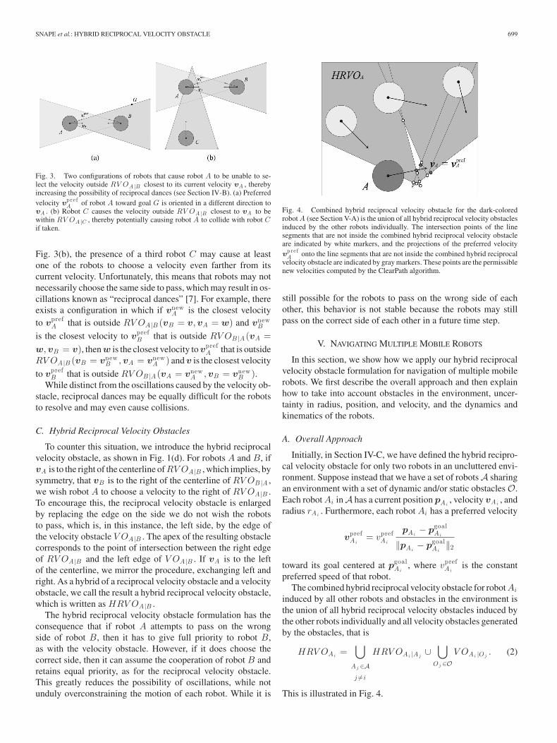
Fig. 4. Combined hybrid reciprocal velocity obstacle for the dark-coloredrobot A (see Section V-A) is the union of all hybrid reciprocal velocity obstaclesinduced by the other robots individually. The intersection points of the linesegments that are not inside the combined hybrid reciprocal velocity obstacleare indicated by white markers, and the projections of the preferred velocityvpref

A onto the line segments that are not inside the combined hybrid reciprocalvelocity obstacle are indicated by gray markers. These points are the permissiblenew velocities computed by the ClearPath algorithm.

still possible for the robots to pass on the wrong side of eachother, this behavior is not stable because the robots may stillpass on the correct side of each other in a future time step.

V. NAVIGATING MULTIPLE MOBILE ROBOTS

In this section, we show how we apply our hybrid reciprocalvelocity obstacle formulation for navigation of multiple mobilerobots. We first describe the overall approach and then explainhow to take into account obstacles in the environment, uncer-tainty in radius, position, and velocity, and the dynamics andkinematics of the robots.

A. Overall Approach

Initially, in Section IV-C, we have defined the hybrid recipro-cal velocity obstacle for only two robots in an uncluttered envi-ronment. Suppose instead that we have a set of robots A sharingan environment with a set of dynamic and/or static obstacles O.Each robot Ai in A has a current position pAi

, velocity vAi, and

radius rAi. Furthermore, each robot Ai has a preferred velocity

vprefAi

= vprefAi

pAi− pgoal

Ai

‖pAi− pgoal

Ai‖2

toward its goal centered at pgoalAi

, where vprefAi

is the constantpreferred speed of that robot.

The combined hybrid reciprocal velocity obstacle for robot Ai

induced by all other robots and obstacles in the environment isthe union of all hybrid reciprocal velocity obstacles induced bythe other robots individually and all velocity obstacles generatedby the obstacles, that is

HRV OAi=

⋃

Aj ∈Aj �=i

HRV OAi |Aj∪

⋃

Oj ∈OV OAi |Oj

. (2)

This is illustrated in Fig. 4.


The robot Ai should, therefore, select as its new velocity vnewAi

the velocity outside the combined hybrid reciprocal velocityobstacle that is closest to its preferred velocity

vnewAi

= arg minv �∈H RV OA i

‖v − vprefAi

‖2 . (3)

We use the ClearPath efficient geometric algorithm [23] tocompute this velocity. Following the ClearPath approach, whichis applicable to many variations of velocity obstacles, we repre-sent the combined hybrid reciprocal velocity obstacle as a unionof line segments. The line segments are intersected pairwise, andthe intersection points inside the combined hybrid reciprocal ve-locity obstacle are discarded. The remaining intersection points,which are shown by white markers in Fig. 4, are permissible newvelocities on the boundary of the combined hybrid reciprocalvelocity obstacle. In addition, we project the preferred velocityvpref

Aionto the line segments, as well as retaining those points

that are outside the combined hybrid reciprocal velocity obsta-cle, as indicated by the gray markers in Fig. 4. It is guaranteedthat the velocity that is closest to the preferred velocity vpref

Aiof

the robot is in either of these two sets [23], and we choose thatpoint as the new velocity for the robot.

If there are no permissible new velocities, we discard the hy-brid reciprocal velocity obstacle of the farthest away robot orobstacle and repeat the ClearPath algorithm until a velocity out-side the combined hybrid reciprocal velocity obstacle becomespermissible. It is possible that there may now be collisions be-tween robots; however, we have only observed this issue onoccasion in simulations with several hundred virtual agents.

While the robot should take the new velocity vnewAi

imme-diately, this may not be directly possible due to its kinematicconstraints. Therefore, the velocity vnew

Aiis transformed into a

control input for the robot that will let the robot assume vnewAi

as soon as possible. We expand upon this transformation inSection V-E.

The overall approach is summarized by the algorithm inFig. 5. Note that we do not require the robots to communi-cate with each other. Robots use only the information that theycan sense independently.

B. Obstacles

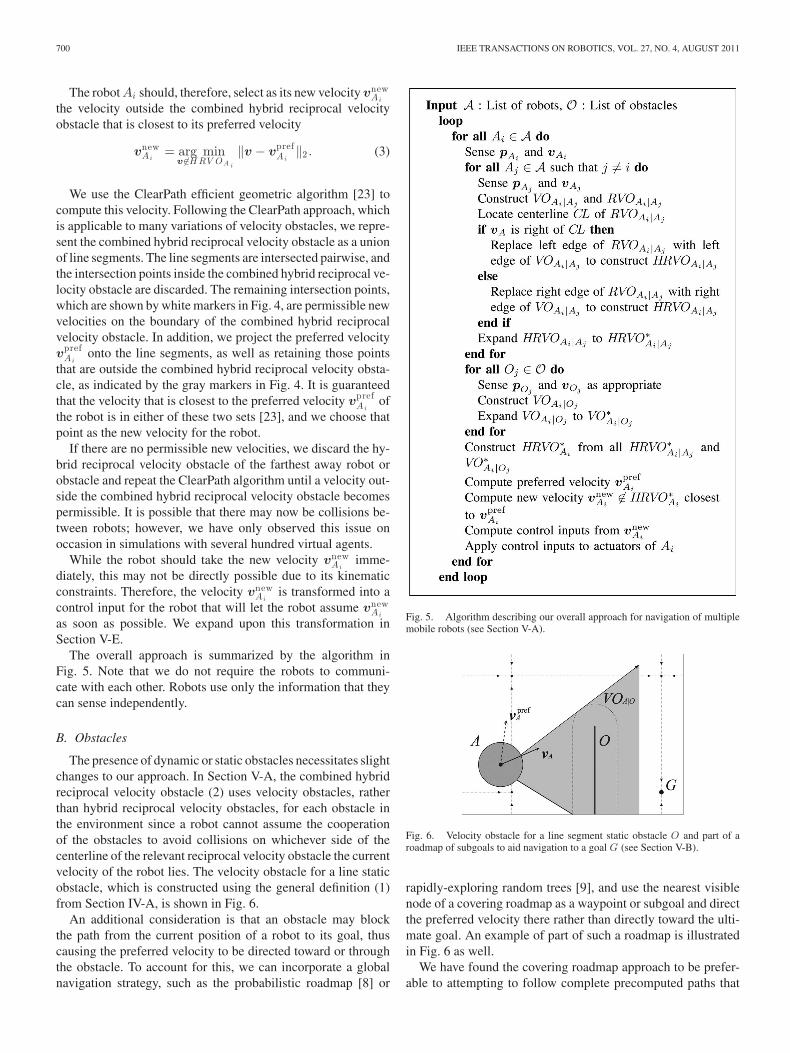
The presence of dynamic or static obstacles necessitates slightchanges to our approach. In Section V-A, the combined hybridreciprocal velocity obstacle (2) uses velocity obstacles, ratherthan hybrid reciprocal velocity obstacles, for each obstacle inthe environment since a robot cannot assume the cooperationof the obstacles to avoid collisions on whichever side of thecenterline of the relevant reciprocal velocity obstacle the currentvelocity of the robot lies. The velocity obstacle for a line staticobstacle, which is constructed using the general definition (1)from Section IV-A, is shown in Fig. 6.

An additional consideration is that an obstacle may blockthe path from the current position of a robot to its goal, thuscausing the preferred velocity to be directed toward or throughthe obstacle. To account for this, we can incorporate a globalnavigation strategy, such as the probabilistic roadmap [8] or

Fig. 5. Algorithm describing our overall approach for navigation of multiplemobile robots (see Section V-A).

Fig. 6. Velocity obstacle for a line segment static obstacle O and part of aroadmap of subgoals to aid navigation to a goal G (see Section V-B).

rapidly-exploring random trees [9], and use the nearest visiblenode of a covering roadmap as a waypoint or subgoal and directthe preferred velocity there rather than directly toward the ulti-mate goal. An example of part of such a roadmap is illustratedin Fig. 6 as well.

We have found the covering roadmap approach to be prefer-able to attempting to follow complete precomputed paths that


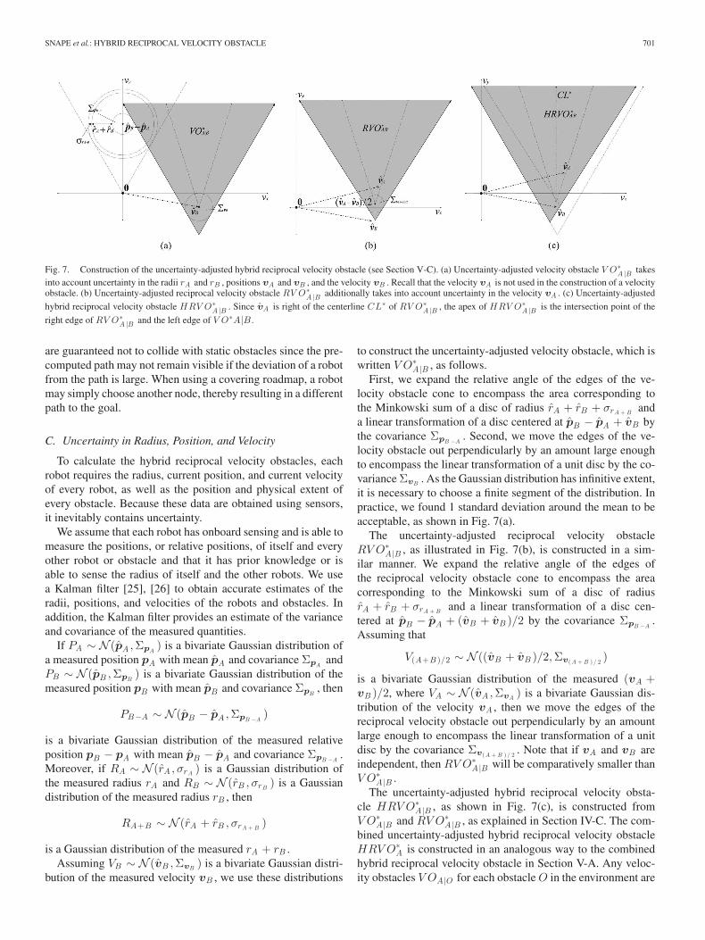
Fig. 7. Construction of the uncertainty-adjusted hybrid reciprocal velocity obstacle (see Section V-C). (a) Uncertainty-adjusted velocity obstacle V O∗A |B takes

into account uncertainty in the radii rA and rB , positions vA and vB , and the velocity vB . Recall that the velocity vA is not used in the construction of a velocityobstacle. (b) Uncertainty-adjusted reciprocal velocity obstacle RV O∗

A |B additionally takes into account uncertainty in the velocity vA . (c) Uncertainty-adjusted

hybrid reciprocal velocity obstacle HRV O∗A |B . Since vA is right of the centerline CL∗ of RV O∗

A |B , the apex of HRV O∗A |B is the intersection point of the

right edge of RV O∗A |B and the left edge of V O∗A|B .

are guaranteed not to collide with static obstacles since the pre-computed path may not remain visible if the deviation of a robotfrom the path is large. When using a covering roadmap, a robotmay simply choose another node, thereby resulting in a differentpath to the goal.

C. Uncertainty in Radius, Position, and Velocity

To calculate the hybrid reciprocal velocity obstacles, eachrobot requires the radius, current position, and current velocityof every robot, as well as the position and physical extent ofevery obstacle. Because these data are obtained using sensors,it inevitably contains uncertainty.

We assume that each robot has onboard sensing and is able tomeasure the positions, or relative positions, of itself and everyother robot or obstacle and that it has prior knowledge or isable to sense the radius of itself and the other robots. We usea Kalman filter [25], [26] to obtain accurate estimates of theradii, positions, and velocities of the robots and obstacles. Inaddition, the Kalman filter provides an estimate of the varianceand covariance of the measured quantities.

If PA ∼ N (pA ,ΣpA) is a bivariate Gaussian distribution of

a measured position pA with mean pA and covariance ΣpAand

PB ∼ N (pB ,ΣpB) is a bivariate Gaussian distribution of the

measured position pB with mean pB and covariance ΣpB, then

PB−A ∼ N (pB − pA ,ΣpB −A)

is a bivariate Gaussian distribution of the measured relativeposition pB − pA with mean pB − pA and covariance ΣpB −A

.Moreover, if RA ∼ N (rA , σrA

) is a Gaussian distribution ofthe measured radius rA and RB ∼ N (rB , σrB

) is a Gaussiandistribution of the measured radius rB , then

RA+B ∼ N (rA + rB , σrA + B)

is a Gaussian distribution of the measured rA + rB .Assuming VB ∼ N (vB ,ΣvB

) is a bivariate Gaussian distri-bution of the measured velocity vB , we use these distributions

to construct the uncertainty-adjusted velocity obstacle, which iswritten V O∗

A |B , as follows.First, we expand the relative angle of the edges of the ve-

locity obstacle cone to encompass the area corresponding tothe Minkowski sum of a disc of radius rA + rB + σrA + B

anda linear transformation of a disc centered at pB − pA + vB bythe covariance ΣpB −A

. Second, we move the edges of the ve-locity obstacle out perpendicularly by an amount large enoughto encompass the linear transformation of a unit disc by the co-variance ΣvB

. As the Gaussian distribution has infinitive extent,it is necessary to choose a finite segment of the distribution. Inpractice, we found 1 standard deviation around the mean to beacceptable, as shown in Fig. 7(a).

The uncertainty-adjusted reciprocal velocity obstacleRV O∗

A |B , as illustrated in Fig. 7(b), is constructed in a sim-ilar manner. We expand the relative angle of the edges ofthe reciprocal velocity obstacle cone to encompass the areacorresponding to the Minkowski sum of a disc of radiusrA + rB + σrA + B

and a linear transformation of a disc cen-tered at pB − pA + (vB + vB )/2 by the covariance ΣpB −A

.Assuming that

V(A+B )/2 ∼ N ((vB + vB )/2,Σv(A + B ) / 2 )

is a bivariate Gaussian distribution of the measured (vA +vB )/2, where VA ∼ N (vA ,ΣvA

) is a bivariate Gaussian dis-tribution of the velocity vA , then we move the edges of thereciprocal velocity obstacle out perpendicularly by an amountlarge enough to encompass the linear transformation of a unitdisc by the covariance Σv(A + B ) / 2 . Note that if vA and vB areindependent, then RV O∗

A |B will be comparatively smaller thanV O∗

A |B .The uncertainty-adjusted hybrid reciprocal velocity obsta-

cle HRV O∗A |B , as shown in Fig. 7(c), is constructed from

V O∗A |B and RV O∗

A |B , as explained in Section IV-C. The com-bined uncertainty-adjusted hybrid reciprocal velocity obstacleHRV O∗

A is constructed in an analogous way to the combinedhybrid reciprocal velocity obstacle in Section V-A. Any veloc-ity obstacles V OA |O for each obstacle O in the environment are


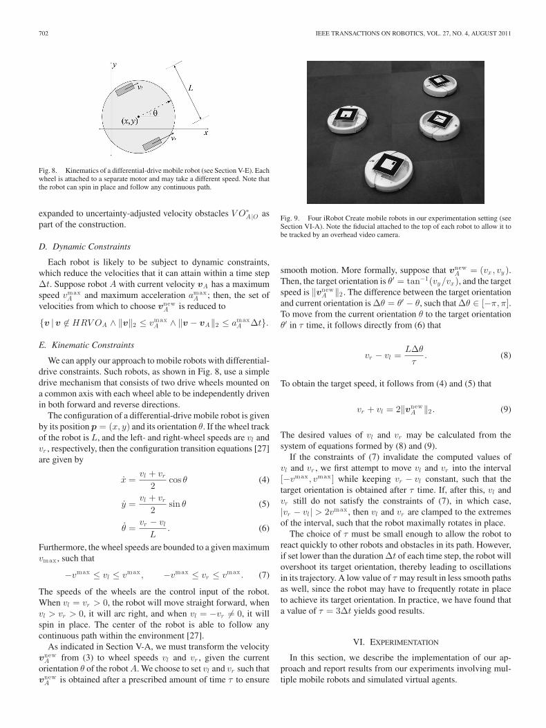
Fig. 8. Kinematics of a differential-drive mobile robot (see Section V-E). Eachwheel is attached to a separate motor and may take a different speed. Note thatthe robot can spin in place and follow any continuous path.

expanded to uncertainty-adjusted velocity obstacles V O∗A |O as

part of the construction.

D. Dynamic Constraints

Each robot is likely to be subject to dynamic constraints,which reduce the velocities that it can attain within a time stepΔt. Suppose robot A with current velocity vA has a maximumspeed vmax

A and maximum acceleration amaxA ; then, the set of

velocities from which to choose vnewA is reduced to

{v |v �∈ HRV OA ∧ ‖v‖2 ≤ vmaxA ∧ ‖v − vA‖2 ≤ amax

A Δt}.

E. Kinematic Constraints

We can apply our approach to mobile robots with differential-drive constraints. Such robots, as shown in Fig. 8, use a simpledrive mechanism that consists of two drive wheels mounted ona common axis with each wheel able to be independently drivenin both forward and reverse directions.

The configuration of a differential-drive mobile robot is givenby its position p = (x, y) and its orientation θ. If the wheel trackof the robot is L, and the left- and right-wheel speeds are vl andvr , respectively, then the configuration transition equations [27]are given by

x =vl + vr

2cos θ (4)

y =vl + vr

2sin θ (5)

θ =vr − vl

L. (6)

Furthermore, the wheel speeds are bounded to a given maximumvmax , such that

−vmax ≤ vl ≤ vmax , −vmax ≤ vr ≤ vmax . (7)

The speeds of the wheels are the control input of the robot.When vl = vr > 0, the robot will move straight forward, whenvl > vr > 0, it will arc right, and when vl = −vr �= 0, it willspin in place. The center of the robot is able to follow anycontinuous path within the environment [27].

As indicated in Section V-A, we must transform the velocityvnew

A from (3) to wheel speeds vl and vr , given the currentorientation θ of the robot A. We choose to set vl and vr such thatvnew

A is obtained after a prescribed amount of time τ to ensure

Fig. 9. Four iRobot Create mobile robots in our experimentation setting (seeSection VI-A). Note the fiducial attached to the top of each robot to allow it tobe tracked by an overhead video camera.

smooth motion. More formally, suppose that vnewA = (vx, vy ).

Then, the target orientation is θ′ = tan−1(vy /vx), and the targetspeed is ‖vnew

A ‖2 . The difference between the target orientationand current orientation is Δθ = θ′ − θ, such that Δθ ∈ [−π, π].To move from the current orientation θ to the target orientationθ′ in τ time, it follows directly from (6) that

vr − vl =LΔθ

τ. (8)

To obtain the target speed, it follows from (4) and (5) that

vr + vl = 2‖vnewA ‖2 . (9)

The desired values of vl and vr may be calculated from thesystem of equations formed by (8) and (9).

If the constraints of (7) invalidate the computed values ofvl and vr , we first attempt to move vl and vr into the interval[−vmax , vmax] while keeping vr − vl constant, such that thetarget orientation is obtained after τ time. If, after this, vl andvr still do not satisfy the constraints of (7), in which case,|vr − vl | > 2vmax , then vl and vr are clamped to the extremesof the interval, such that the robot maximally rotates in place.

The choice of τ must be small enough to allow the robot toreact quickly to other robots and obstacles in its path. However,if set lower than the duration Δt of each time step, the robot willovershoot its target orientation, thereby leading to oscillationsin its trajectory. A low value of τ may result in less smooth pathsas well, since the robot may have to frequently rotate in placeto achieve its target orientation. In practice, we have found thata value of τ = 3Δt yields good results.

VI. EXPERIMENTATION

In this section, we describe the implementation of our ap-proach and report results from our experiments involving mul-tiple mobile robots and simulated virtual agents.


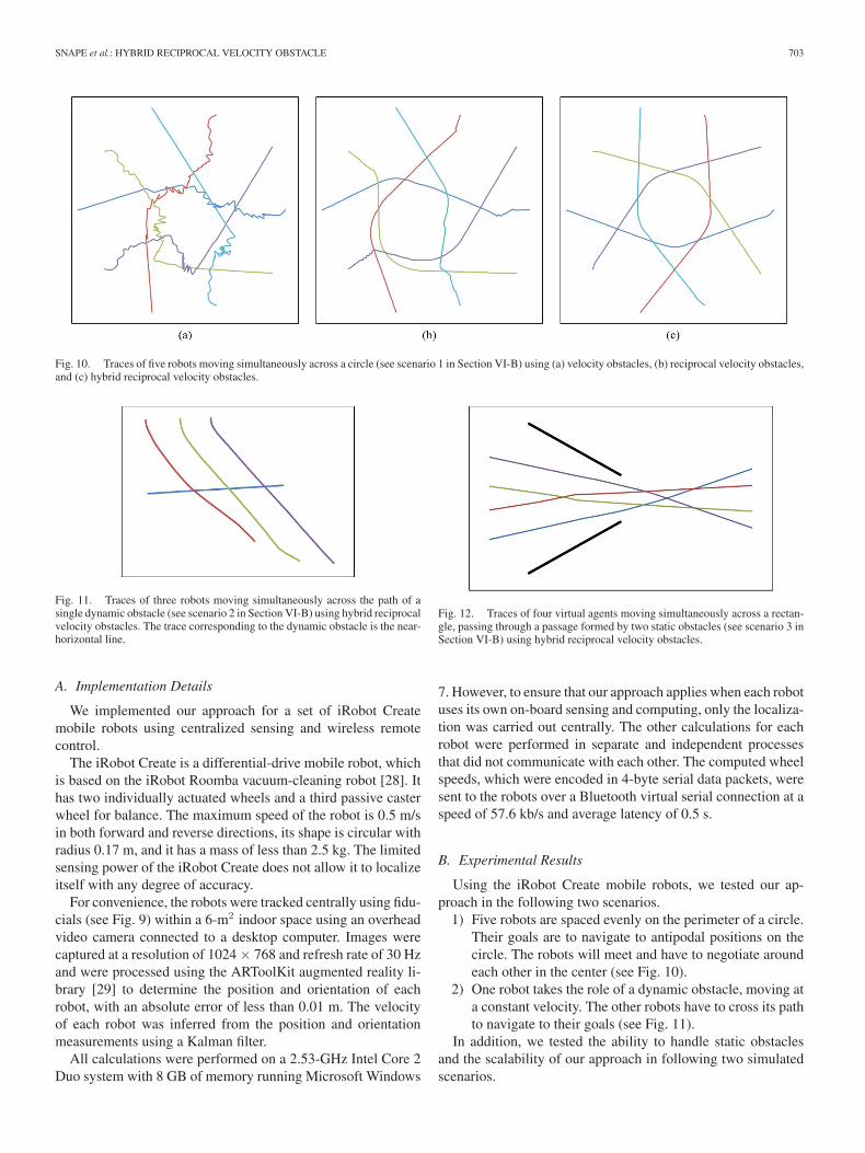
Fig. 10. Traces of five robots moving simultaneously across a circle (see scenario 1 in Section VI-B) using (a) velocity obstacles, (b) reciprocal velocity obstacles,and (c) hybrid reciprocal velocity obstacles.

Fig. 11. Traces of three robots moving simultaneously across the path of asingle dynamic obstacle (see scenario 2 in Section VI-B) using hybrid reciprocalvelocity obstacles. The trace corresponding to the dynamic obstacle is the near-horizontal line.

A. Implementation Details

We implemented our approach for a set of iRobot Createmobile robots using centralized sensing and wireless remotecontrol.

The iRobot Create is a differential-drive mobile robot, whichis based on the iRobot Roomba vacuum-cleaning robot [28]. Ithas two individually actuated wheels and a third passive casterwheel for balance. The maximum speed of the robot is 0.5 m/sin both forward and reverse directions, its shape is circular withradius 0.17 m, and it has a mass of less than 2.5 kg. The limitedsensing power of the iRobot Create does not allow it to localizeitself with any degree of accuracy.

For convenience, the robots were tracked centrally using fidu-cials (see Fig. 9) within a 6-m2 indoor space using an overheadvideo camera connected to a desktop computer. Images werecaptured at a resolution of 1024 × 768 and refresh rate of 30 Hzand were processed using the ARToolKit augmented reality li-brary [29] to determine the position and orientation of eachrobot, with an absolute error of less than 0.01 m. The velocityof each robot was inferred from the position and orientationmeasurements using a Kalman filter.

All calculations were performed on a 2.53-GHz Intel Core 2Duo system with 8 GB of memory running Microsoft Windows

Fig. 12. Traces of four virtual agents moving simultaneously across a rectan-gle, passing through a passage formed by two static obstacles (see scenario 3 inSection VI-B) using hybrid reciprocal velocity obstacles.

7. However, to ensure that our approach applies when each robotuses its own on-board sensing and computing, only the localiza-tion was carried out centrally. The other calculations for eachrobot were performed in separate and independent processesthat did not communicate with each other. The computed wheelspeeds, which were encoded in 4-byte serial data packets, weresent to the robots over a Bluetooth virtual serial connection at aspeed of 57.6 kb/s and average latency of 0.5 s.

B. Experimental Results

Using the iRobot Create mobile robots, we tested our ap-proach in the following two scenarios.

1) Five robots are spaced evenly on the perimeter of a circle.Their goals are to navigate to antipodal positions on thecircle. The robots will meet and have to negotiate aroundeach other in the center (see Fig. 10).

2) One robot takes the role of a dynamic obstacle, moving ata constant velocity. The other robots have to cross its pathto navigate to their goals (see Fig. 11).

In addition, we tested the ability to handle static obstaclesand the scalability of our approach in following two simulatedscenarios.


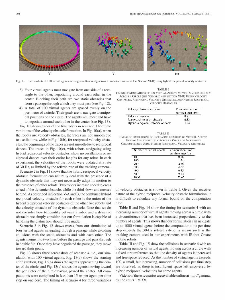
Fig. 13. Screenshots of 100 virtual agents moving simultaneously across a circle (see scenario 4 in Section VI-B) using hybrid reciprocal velocity obstacles.

3) Four virtual agents must navigate from one side of a rect-angle to the other, negotiating around each other in thecenter. Blocking their path are two static obstacles thatform a passage through which they must pass (see Fig. 12).

4) A total of 100 virtual agents are spaced evenly on theperimeter of a circle. Their goals are to navigate to antipo-dal positions on the circle. The agents will meet and haveto negotiate around each other in the center (see Fig. 13).

Fig. 10 shows traces of the five robots in scenario 1 for threevariations of the velocity obstacle formation. In Fig. 10(a), whenthe robots use velocity obstacles, the traces are not smooth dueto oscillations, while in Fig. 10(b), for reciprocal velocity obsta-cles, the beginnings of the traces are not smooth due to reciprocaldances. The traces in Fig. 10(c), with robots navigating usinghybrid reciprocal velocity obstacles, show no oscillations or re-ciprocal dances over their entire lengths for any robot. In eachexperiment, the velocities of the robots were updated at a rateof 30 Hz, as limited by the refresh rate of the tracking camera.

Scenario 2 in Fig. 11 shows that the hybrid reciprocal velocityobstacle formulation can naturally deal with the presence of adynamic obstacle that may not necessarily adapt its motion tothe presence of other robots. Two robots increase speed to crossahead of the dynamic obstacle, while the third slows and crossesbehind. As described in Section V-A and B, the combined hybridreciprocal velocity obstacle for each robot is the union of thehybrid reciprocal velocity obstacles of the other two robots andthe velocity obstacle of the dynamic obstacle. Note that we donot consider how to identify between a robot and a dynamicobstacle; we simply consider that our formulation is capable ofhandling the distinction should it be made.

Scenario 3 in Fig. 12 shows traces from our simulation offour virtual agents navigating though a passage while avoidingcollisions with the static obstacles and with each other. Theagents merge into two lines before the passage and pass throughin double file. Once they have negotiated the passage, they movetoward their goals.

Fig. 13 shows three screenshots of scenario 4, i.e., our sim-ulation with 100 virtual agents. Fig. 13(a) shows the startingconfiguration, Fig. 13(b) shows the agents approaching the cen-ter of the circle, and Fig. 13(c) shows the agents moving towardthe perimeter of the circle having passed the center. All com-putations were completed in less than 15 μs per agent per timestep on one core. The timing of scenario 4 for three variations

TABLE ITIMING OF SIMULATIONS OF 100 VIRTUAL AGENTS MOVING SIMULTANEOUSLY

ACROSS A CIRCLE (SEE SCENARIO 4 IN SECTION VI-B) USING VELOCITY

OBSTACLES, RECIPROCAL VELOCITY OBSTACLES, AND HYBRID RECIPROCAL

VELOCITY OBSTACLES

TABLE IITIMING OF SIMULATIONS OF INCREASING NUMBERS OF VIRTUAL AGENTS

MOVING SIMULTANEOUSLY ACROSS A CIRCLE OF INCREASING

CIRCUMFERENCE USING HYBRID RECIPROCAL VELOCITY OBSTACLES

of velocity obstacles is shown in Table I. Given the reactivenature of the hybrid reciprocal velocity obstacle formulation, itis difficult to calculate any formal bound on the computationtime.

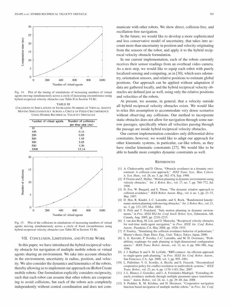
Table II and Fig. 14 show the timing for scenario 4 with anincreasing number of virtual agents moving across a circle witha circumference that has been increased proportionally to thenumber of agents. This shows that our formulation can navigateup to 1000 virtual agents before the computation time per timestep exceeds the 30-Hz refresh rate of a sensor such as thetracking camera used in our experiments with iRobot Createmobile robots.

Table III and Fig. 15 show the collisions in scenario 4 with anincreasing number of virtual agents moving across a circle witha fixed circumference so that the density of agents is increasedand free space reduced. As the number of virtual agents exceeds100, a small, but increasing, number of collisions per time stepare observed, as there is insufficient space left uncovered byhybrid reciprocal velocities for some agents.

Videos of these scenarios are available online at http://gamma.cs.unc.edu/HRV O/.


Fig. 14. Plot of the timing of simulations of increasing numbers of virtualagents moving simultaneously across a circle of increasing circumference usinghybrid reciprocal velocity obstacles (see Table II in Section VI-B).

TABLE IIICOLLISIONS IN SIMULATIONS OF INCREASING NUMBERS OF VIRTUAL AGENTS

MOVING SIMULTANEOUSLY ACROSS A CIRCLE OF FIXED CIRCUMFERENCE

USING HYBRID RECIPROCAL VELOCITY OBSTACLES

Fig. 15. Plot of the collisions in simulations of increasing numbers of virtualagents moving simultaneously across a circle of fixed circumference usinghybrid reciprocal velocity obstacles (see Table III in Section VI-B).

VII. CONCLUSION, LIMITATIONS, AND FUTURE WORK

In this paper, we have introduced the hybrid reciprocal veloc-ity obstacle for navigation of multiple mobile robots or virtualagents sharing an environment. We take into account obstaclesin the environment, uncertainty in radius, position, and veloc-ity. We also consider the dynamics and kinematics of the robots,thereby allowing us to implement our approach on iRobot Createmobile robots. Our formulation explicitly considers reciprocity,such that each robot can assume that other robots are cooperat-ing to avoid collisions, but each of the robots acts completelyindependently without central coordination and does not com-

municate with other robots. We show direct, collision-free, andoscillation-free navigation.

In the future, we would like to develop a more sophisticatedand less conservative model of uncertainty, that takes into ac-count more than uncertainty in position and velocity originatingfrom the sensors of the robot, and apply it to the hybrid recip-rocal velocity obstacle formulation.

In our current implementation, each of the robots currentlyreceives their sensor readings from an overhead video camera.As a next step, we would like to equip each robot with purelylocalized sensing and computing, as in [30], which uses odome-try, orientation sensors, and relative positions to estimate globalpositions. Our approach can be applied without adaptation ifdata are gathered locally, and the hybrid reciprocal velocity ob-stacles are defined just as well, using only the relative positionsand velocities of the robots.

At present, we assume, in general, that a velocity outsideall hybrid reciprocal velocity obstacles exists. We would liketo relax this assumption to accommodate very dense scenarioswithout observing any collisions. Our method to incorporatestatic obstacles does not allow for navigation through some nar-row passages, specifically where all velocities passing throughthe passage are inside hybrid reciprocal velocity obstacles.

Our current implementation considers only differential-driveconstraints; however, we would like to adapt our approach forother kinematic systems, in particular, car-like robots, as theyhave similar kinematic constraints [27]. We would like to beable to handle more complex dynamic constraints as well.

REFERENCES

[1] A. Chakravarthy and D. Ghose, “Obstacle avoidance in a dynamic envi-ronment: A collision cone approach,” IEEE Trans. Syst., Man, Cybern.A, Syst. Hum., vol. 28, no. 5, pp. 562–574, Sep. 1998.

[2] P. Fiorini and Z. Shiller, “Motion planning in dynamic environments usingvelocity obstacles,” Int. J. Robot. Res., vol. 17, no. 7, pp. 760–772, Jul.1998.

[3] D. Fox, W. Burgard, and S. Thrun, “The dynamic window approach tocollision avoidance,” IEEE Robot. Autom. Mag., vol. 4, no. 1, pp. 23–33,Mar. 1997.

[4] D. Hsu, R. Kindel, J.-C. Latombe, and S. Rock, “Randomized kinody-namic motion planning with moving obstacles,” Int. J. Robot. Res., vol. 21,no. 3, pp. 233–255, Mar. 2002.

[5] S. Petti and T. Fraichard, “Safe motion planning in dynamic environ-ments,” in Proc. IEEE RSJ Int. Conf. Intell. Robot. Syst., Edmonton, AB,Canada, Aug. 2005, pp. 2210–2215.

[6] J. van den Berg, M. Lin, and D. Manocha, “Reciprocal velocity obstaclesfor real-time multi-agent navigation,” in Proc. IEEE Int. Conf. Robot.Autom., Pasadena, CA, May 2008, pp. 1928–1935.

[7] F. Feurtey, “Simulating the collision avoidance behavior of pedestrians,”Master’s thesis, Dept. Elect. Eng., Univ. Tokyo, Tokyo, Japan, 2000.

[8] L. E. Kavraki, P. Svestka, J.-C. Latombe, and M. H. Overmars, “Prob-abilistic roadmaps for path planning in high-dimensional configurationspaces,” IEEE Trans. Robot. Autom., vol. 12, no. 4, pp. 566–580, Aug.1996.

[9] J. J. Kuffner Jr and S. M. LaValle, “RRT-connect: An efficient approachto single-query path planning,” in Proc. IEEE Int. Conf. Robot. Autom.,San Francisco, CA, Apr. 2000, vol. 2, pp. 995–1001.

[10] L. Pallottino, V. G. Scordio, A. Bicchi, and E. Frazzoli, “Decentralizedcooperative policy for conflict resolution in multivehicle systems,” IEEETrans. Robot., vol. 23, no. 6, pp. 1170–1183, Dec. 2007.

[11] J.-L. Blanco, J. Gonzalez, and J.-A. Fernandez-Madrigal, “Extending ob-stacle avoidance methods through multiple parameter-space transforma-tions,” Auton. Robot., vol. 24, no. 1, pp. 29–48, Jan. 2008.

[12] S. Pedduri, K. M. Krishna, and H. Hexmoor, “Cooperative navigationfunction based navigation of multiple mobile robots,” in Proc. Int. Conf.


Integr. Knowl. Intensive Multi-Agent Syst., Waltham, MA, Apr./May 2007,pp. 277–282.

[13] K. E. Bekris, K. I. Tsianos, and L. E. Kavraki, “A decentralized planner thatguarantees the safety of communicating vehicles with complex dynamicsthat replan online,” in Proc. IEEE RSJ Int. Conf. Intell. Robot. Syst., SanDiego, CA, Oct./Nov. 2007, pp. 3784–3790.

[14] F. Large, S. Sckhavat, Z. Shiller, and C. Laugier, “Using non-linear ve-locity obstacles to plan motions in a dynamic environment,” in Proc.IEEE Int. Conf. Contr. Autom. Robot. Vis., Singapore, Dec. 2002, vol. 2,pp. 734–739.

[15] Z. Shiller, R. Prasanna, and J. Salinger, “A unified approach to forwardand lane-change collision warning for driver assistance and situationalawareness,” in Intelligent Vehicle Initiative (IVI) Technology Controls andNavigation Systems. Warrendale, PA: SAE Int., Apr. 2008, Paper 2008-01-0204.

[16] E. Prassler, J. Scholz, and P. Fiorini, “Navigating a robotic wheelchair ina railway station during rush hour,” Int. J. Robot. Res., vol. 18, no. 7,pp. 711–727, Jul. 1999.

[17] P. Fiorini and D. Botturi, “Introducing service robotics to the pharma-ceutical industry,” Intell. Serv. Robot., vol. 1, no. 4, pp. 267–280, Oct.2008.

[18] J. S. Dittrich, F. Adolf, A. Langer, and F. Thielecke, “Mission planningfor low-flying unmanned rotorcraft in uncertain environments,” presentedat AHS Int. Spec. Mtg. Unmanned Rotorcraft, Chandler, AZ, Jan. 2007.

[19] Y. Abe and M. Yoshiki, “Collision avoidance method for multiple au-tonomous mobile agents by implicit cooperation,” in Proc. IEEE RSJ Int.Conf. Intell. Robot. Syst., vol. 3, Maui, HI, Oct./Nov. 2001, pp. 1207–1212.

[20] B. Kluge and E. Prassler, “Recursive probabilistic velocity obstacles forreflective navigation,” in Field and Service Robotics: Recent Advances inResearch and Applications, (Springer Tracts in Advanced Robotics, vol.24), S. Yuta, H. Asama, S. Thrun, E. Prassler, and T. Tsubouchi, Eds.Berlin, Germany: Springer-Verlag, Jul. 2006, pp. 71–79.

[21] C. Fulgenzi, A. Spalanzani, and C. Laugier, “Dynamic obstacle avoidancein uncertain environment combining PVOs and occupancy grid,” in Proc.IEEE Int. Conf. Robot. Autom., Rome, Italy, Apr. 2007, pp. 1610–1616.

[22] O. Gal, Z. Shiller, and E. Rimon, “Efficient and safe on-line motion plan-ning in dynamic environments,” in Proc. IEEE Int. Conf. Robot. Autom.,Kobe, Japan, May 2009, pp. 88–93.

[23] S. J. Guy, J. Chhugani, C. Kim, N. Satish, M. Lin, D. Manocha, andP. Dubey, “ClearPath: Highly parallel collision avoidance for multi-agentsimulation,” in Proc. ACM SIGGRAPH Eurographics Symp. Comput. An-imat., New Orleans, LA, Aug. 2009, pp. 177–187.

[24] J. van den Berg, S. J. Guy, M. Lin, and D. Manocha, “Reciprocaln-body collision avoidance,” in Robotics Research: The 14th Interna-tional Symposium ISRR, (Springer Tracts in Advanced Robotics, vol. 70),C. Pradalier, R. Siegwart, and G. Hirzinger, Eds. Berlin, Germany:Springer-Verlag, Apr. 2011.

[25] R. E. Kalman, “A new approach to linear filtering and prediction prob-lems,” Trans. ASME—J. Basic Eng., vol. 82, pp. 35–45, Mar. 1960.

[26] G. Welch and G. Bishop, “An introduction to the Kalman filter,” Dept.Comput. Sci., Univ. North Carolina Chapel Hill, Chapel Hill, NC, Tech.Rep. 95-041, 1995.

[27] S. M. LaValle, Planning Algorithms. Cambridge, U.K.: CambridgeUniv. Press, May 2006, ch. 13, pp. 590–650.

[28] J. L. Jones, N. E. Mack, D. M. Nugent, and P. E. Sandin, “Autonomousfloor-cleaning robot,” U.S. Patent 6 883 201, Apr. 26, 2005.

[29] H. Kato and M. Billinghurst, “Marker tracking and HMD calibration for avideo-based augmented reality conferencing system,” in Proc. IEEE ACMInt. Workshop Augment. Real., San Francisco, CA, Oct. 1999, pp. 85–94.

[30] S. I. Roumeliotis and I. M. Rekleitis, “Propagation of uncertainty in coop-erative multirobot localization: Analysis and experimental results,” Auton.Robot., vol. 17, no. 1, pp. 41–54, Jul. 2004.

Jamie Snape (S’09) received the M.Math. (Hons.)degree in mathematics from Collingwood College,University of Durham, Durham, U.K., in 2004, theM.Sc. degree in computer science from WorcesterCollege, University of Oxford, Oxford, U.K., in 2005,and the M.S. degree in 2009 in computer sciencefrom the University of North Carolina at Chapel Hill,where he is currently working toward the Ph.D. de-gree with the Department of Computer Science.

He was a Systems Developer with MillenniumGlobal Investments Ltd., London, U.K. His current

research interests include motion and path planning, multirobot systems, andmobile robotics.

Jur van den Berg received the M.Sc. degree incomputer science from the University of Groningen,Groningen, the Netherlands, in 2003 and the Ph.D.degree in computer science from the University ofUtrecht, Utrecht, the Netherlands, in 2007.

He is currently a Postdoctoral Research Associatewith the Department of Computer Science, Universityof North Carolina at Chapel Hill. He was a Postdoc-toral Research Associate with the Department of In-dustrial Engineering and Operations Research, Uni-versity of California, Berkeley. His current research

interests include motion and path planning, navigation of virtual characters, andmedical robotics.

Stephen J. Guy received the B.S. degree in com-puter engineering from the University of Virginia,Charlottesville, in 2006 and the M.S. degree in 2009in computer science from the University of NorthCarolina at Chapel Hill, where he is currently work-ing toward the Ph.D. degree with the Department ofComputer Science.

He was an Intern with NVIDIA Corporation,Durham, NC, and with Intel Corporation, Santa Clara,CA. His current research interests include motionand path planning, crowd simulation, and many-core

computing.Mr. Guy is the recipient of the National Science Foundation AGEP Fellow-

ship, the Intel Corporation GEM Fellowship, and the United Negro CollegeFund Google Scholarship.

Dinesh Manocha received the B.E. degree in com-puter science and engineering from the Indian Insti-tute of Technology Delhi, New Delhi, India, in 1987and the M.S. and Ph.D. degrees in computer sciencefrom the University of California, Berkeley, in 1990and 1992, respectively.

He is currently the Phi Delta Theta/Matthew Ma-son Distinguished Professor of computer science withthe Department of Computer Science, University ofNorth Carolina at Chapel Hill. His current researchinterests include geometric computing, interactive

computer graphics, physics-based simulation, and robotics.Prof. Manocha is a Fellow of the American Association for the Advancement

of Science and the Association for Computing Machinery. He is the recipientof the Alfred P. Sloan Research Fellowship, the National Science FoundationCAREER Award, the Office of Naval Research Young Investigator Award, theHonda Initiation Grant, the Phillip and Ruth Hettleman Prize for Artistic andScholarly Achievement by Young Faculty with the University of North Carolinaat Chapel Hill, and the NVIDIA Professor Partnership Award.

Documents

696 IEEE TRANSACTIONS ON ROBOTICS, VOL. 27, NO. 4, AUGUST