Embed Size (px)
Citation preview
6a. Measure & Conquer
COMP6741: Parameterized and Exact Computation
Serge Gaspers12
1School of Computer Science and Engineering, UNSW Sydney, Australia2Decision Sciences, Data61, CSIRO, Australia
Semester 2, 2018
S. Gaspers (UNSW) Measure & Conquer Semester 2, 2018 1 / 48

Outline
1 Introduction
2 Maximum Independent SetSimple AnalysisSearch Trees and Branching NumbersMeasure & Conquer AnalysisOptimizing the measureExponential Time SubroutinesStructures that arise rarely
3 Further Reading
S. Gaspers (UNSW) Measure & Conquer Semester 2, 2018 2 / 48
Outline
1 Introduction
2 Maximum Independent SetSimple AnalysisSearch Trees and Branching NumbersMeasure & Conquer AnalysisOptimizing the measureExponential Time SubroutinesStructures that arise rarely
3 Further Reading
S. Gaspers (UNSW) Measure & Conquer Semester 2, 2018 3 / 48
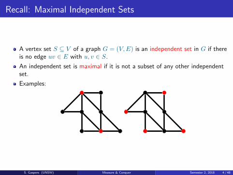
Recall: Maximal Independent Sets
A vertex set S ⊆ V of a graph G = (V,E) is an independent set in G if thereis no edge uv ∈ E with u, v ∈ S.
An independent set is maximal if it is not a subset of any other independentset.
Examples:
S. Gaspers (UNSW) Measure & Conquer Semester 2, 2018 4 / 48
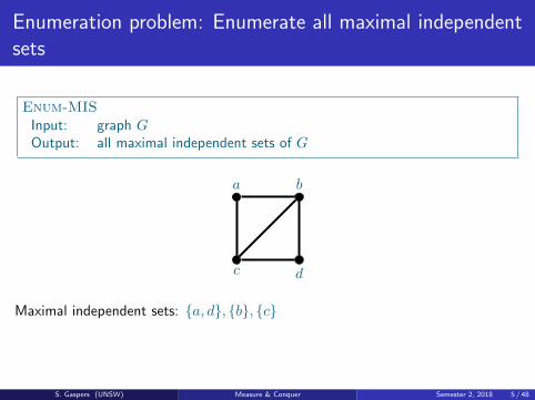
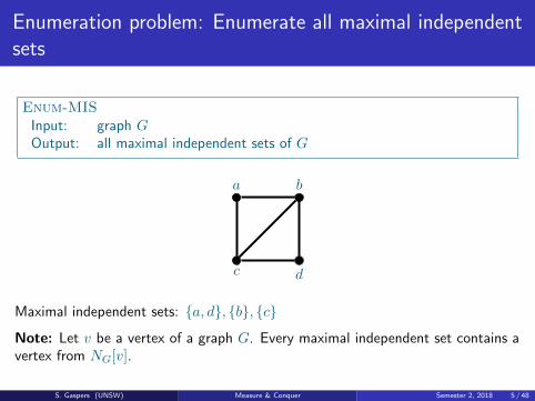
Enumeration problem: Enumerate all maximal independentsets
Enum-MISInput: graph GOutput: all maximal independent sets of G
a b
c d
Maximal independent sets: a, d, b, c
Note: Let v be a vertex of a graph G. Every maximal independent set contains avertex from NG[v].
S. Gaspers (UNSW) Measure & Conquer Semester 2, 2018 5 / 48
Branching Algorithm for Enum-MIS
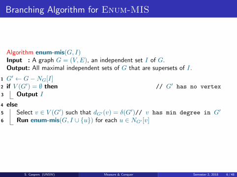
Algorithm enum-mis(G, I)Input : A graph G = (V,E), an independent set I of G.Output: All maximal independent sets of G that are supersets of I.
1 G′ ← G−NG[I]2 if V (G′) = ∅ then // G′ has no vertex
3 Output I
4 else5 Select v ∈ V (G′) such that dG′(v) = δ(G′)// v has min degree in G′
6 Run enum-mis(G, I ∪ u) for each u ∈ NG′ [v]
S. Gaspers (UNSW) Measure & Conquer Semester 2, 2018 6 / 48
Running Time Analysis
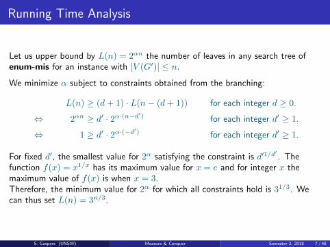
Let us upper bound by L(n) = 2αn the number of leaves in any search tree ofenum-mis for an instance with |V (G′)| ≤ n.
We minimize α subject to constraints obtained from the branching:
L(n) ≥ (d+ 1) · L(n− (d+ 1)) for each integer d ≥ 0.
⇔ 2αn ≥ d′ · 2α·(n−d′) for each integer d′ ≥ 1.
⇔ 1 ≥ d′ · 2α·(−d′) for each integer d′ ≥ 1.
For fixed d′, the smallest value for 2α satisfying the constraint is d′1/d′. The
function f(x) = x1/x has its maximum value for x = e and for integer x themaximum value of f(x) is when x = 3.Therefore, the minimum value for 2α for which all constraints hold is 31/3. Wecan thus set L(n) = 3n/3.
S. Gaspers (UNSW) Measure & Conquer Semester 2, 2018 7 / 48
Running Time Analysis II
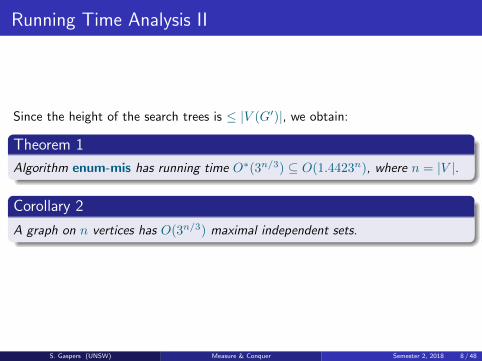
Since the height of the search trees is ≤ |V (G′)|, we obtain:
Theorem 1
Algorithm enum-mis has running time O∗(3n/3) ⊆ O(1.4423n), where n = |V |.
Corollary 2
A graph on n vertices has O(3n/3) maximal independent sets.
S. Gaspers (UNSW) Measure & Conquer Semester 2, 2018 8 / 48
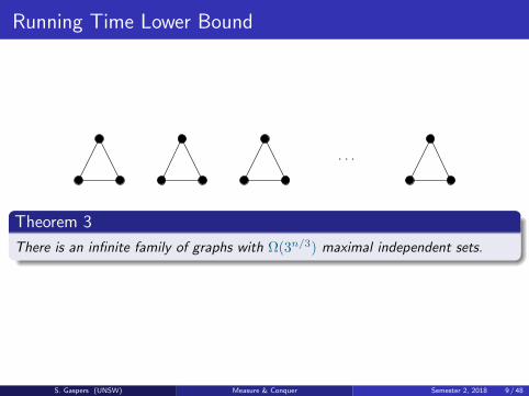
Running Time Lower Bound
· · ·
Theorem 3
There is an infinite family of graphs with Ω(3n/3) maximal independent sets.
S. Gaspers (UNSW) Measure & Conquer Semester 2, 2018 9 / 48
Outline
1 Introduction
2 Maximum Independent SetSimple AnalysisSearch Trees and Branching NumbersMeasure & Conquer AnalysisOptimizing the measureExponential Time SubroutinesStructures that arise rarely
3 Further Reading
S. Gaspers (UNSW) Measure & Conquer Semester 2, 2018 10 / 48
Maximum Independent Set
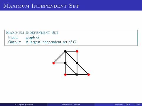
Maximum Independent SetInput: graph GOutput: A largest independent set of G.
S. Gaspers (UNSW) Measure & Conquer Semester 2, 2018 11 / 48
Branching Algorithm for Maximum Independent Set
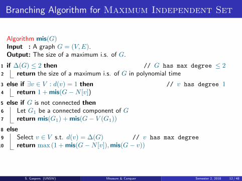
Algorithm mis(G)Input : A graph G = (V,E).Output: The size of a maximum i.s. of G.
1 if ∆(G) ≤ 2 then // G has max degree ≤ 22 return the size of a maximum i.s. of G in polynomial time
3 else if ∃v ∈ V : d(v) = 1 then // v has degree 14 return 1 + mis(G−N [v])
5 else if G is not connected then6 Let G1 be a connected component of G7 return mis(G1) + mis(G− V (G1))
8 else9 Select v ∈ V s.t. d(v) = ∆(G) // v has max degree
10 return max (1 + mis(G−N [v]),mis(G− v))
S. Gaspers (UNSW) Measure & Conquer Semester 2, 2018 12 / 48
Correctness
Line 4:
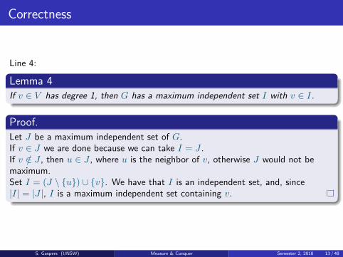
Lemma 4If v ∈ V has degree 1, then G has a maximum independent set I with v ∈ I.
Proof.Let J be a maximum independent set of G.If v ∈ J we are done because we can take I = J .If v /∈ J , then u ∈ J , where u is the neighbor of v, otherwise J would not bemaximum.Set I = (J \ u) ∪ v. We have that I is an independent set, and, since|I| = |J |, I is a maximum independent set containing v.
S. Gaspers (UNSW) Measure & Conquer Semester 2, 2018 13 / 48
Outline
1 Introduction
2 Maximum Independent SetSimple AnalysisSearch Trees and Branching NumbersMeasure & Conquer AnalysisOptimizing the measureExponential Time SubroutinesStructures that arise rarely
3 Further Reading
S. Gaspers (UNSW) Measure & Conquer Semester 2, 2018 14 / 48
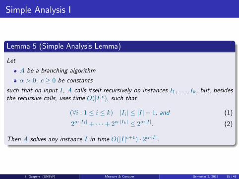
Simple Analysis I
Lemma 5 (Simple Analysis Lemma)
Let
A be a branching algorithm
α > 0, c ≥ 0 be constants
such that on input I, A calls itself recursively on instances I1, . . . , Ik, but, besidesthe recursive calls, uses time O(|I|c), such that
(∀i : 1 ≤ i ≤ k) |Ii| ≤ |I| − 1, and (1)
2α·|I1| + · · ·+ 2α·|Ik| ≤ 2α·|I|. (2)
Then A solves any instance I in time O(|I|c+1) · 2α·|I|.
S. Gaspers (UNSW) Measure & Conquer Semester 2, 2018 15 / 48
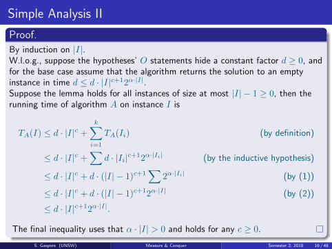
Simple Analysis II
Proof.
By induction on |I|.W.l.o.g., suppose the hypotheses’ O statements hide a constant factor d ≥ 0, andfor the base case assume that the algorithm returns the solution to an emptyinstance in time d ≤ d · |I|c+12α·|I|.Suppose the lemma holds for all instances of size at most |I| − 1 ≥ 0, then therunning time of algorithm A on instance I is
TA(I) ≤ d · |I|c +
k∑i=1
TA(Ii) (by definition)
≤ d · |I|c +∑
d · |Ii|c+12α·|Ii| (by the inductive hypothesis)
≤ d · |I|c + d · (|I| − 1)c+1∑
2α·|Ii| (by (1))
≤ d · |I|c + d · (|I| − 1)c+12α·|I| (by (2))
≤ d · |I|c+12α·|I|.
The final inequality uses that α · |I| > 0 and holds for any c ≥ 0.
S. Gaspers (UNSW) Measure & Conquer Semester 2, 2018 16 / 48
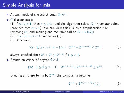
Simple Analysis for mis
At each node of the search tree: O(n2)
G disconnected:(1) If α · s < 1, then s < 1/α, and the algorithm solves G1 in constant time(provided that α > 0). We can view this rule as a simplification rule,removing G1 and making one recursive call on G− V (G1).(2) If α · (n− s) < 1: similar as (1).(3) Otherwise,
(∀s : 1/α ≤ s ≤ n− 1/α) 2α·s + 2α·(n−s) ≤ 2α·n. (3)
always satisfied since 2x + 2y ≤ 2x+y if x, y ≥ 1.
Branch on vertex of degree d ≥ 3
(∀d : 3 ≤ d ≤ n− 1) 2α·(n−1) + 2α·(n−1−d) ≤ 2αn. (4)
Dividing all these terms by 2αn, the constraints become
2−α + 2α·(−1−d) ≤ 1. (5)
S. Gaspers (UNSW) Measure & Conquer Semester 2, 2018 17 / 48
Compute optimum α
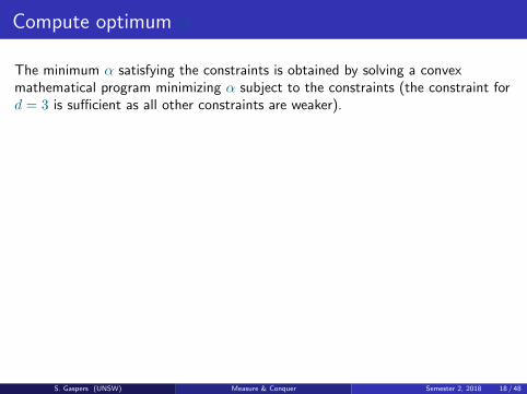
The minimum α satisfying the constraints is obtained by solving a convexmathematical program minimizing α subject to the constraints (the constraint ford = 3 is sufficient as all other constraints are weaker).
Alternatively, set x := 2α, compute the unique positive real root of each of thecharacteristic polynomials
cd(x) := x−1 + x−1−d − 1,
and take the maximum of these roots [Kullmann ’99].
d x α3 1.3803 0.46504 1.3248 0.40575 1.2852 0.36206 1.2555 0.32827 1.2321 0.3011
S. Gaspers (UNSW) Measure & Conquer Semester 2, 2018 18 / 48
Compute optimum α
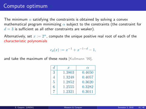
The minimum α satisfying the constraints is obtained by solving a convexmathematical program minimizing α subject to the constraints (the constraint ford = 3 is sufficient as all other constraints are weaker).
Alternatively, set x := 2α, compute the unique positive real root of each of thecharacteristic polynomials
cd(x) := x−1 + x−1−d − 1,
and take the maximum of these roots [Kullmann ’99].
d x α3 1.3803 0.46504 1.3248 0.40575 1.2852 0.36206 1.2555 0.32827 1.2321 0.3011
S. Gaspers (UNSW) Measure & Conquer Semester 2, 2018 18 / 48
Simple Analysis: Result
use the Simple Analysis Lemma with c = 2 and α = 0.464959
running time of Algorithm mis upper bounded byO(n3) · 20.464959·n = O(20.4650·n) or O(1.3803n)
S. Gaspers (UNSW) Measure & Conquer Semester 2, 2018 19 / 48
Lower bound
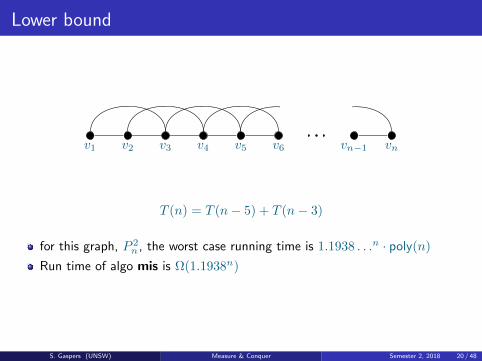
v1 v2 v3 v4 v5 v6 vn−1 vn
T (n) = T (n− 5) + T (n− 3)
for this graph, P 2n , the worst case running time is 1.1938 . . .n · poly(n)
Run time of algo mis is Ω(1.1938n)
S. Gaspers (UNSW) Measure & Conquer Semester 2, 2018 20 / 48
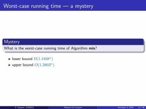
Worst-case running time — a mystery
Mystery
What is the worst-case running time of Algorithm mis?
lower bound Ω(1.1938n)
upper bound O(1.3803n)
S. Gaspers (UNSW) Measure & Conquer Semester 2, 2018 21 / 48
Outline
1 Introduction
2 Maximum Independent SetSimple AnalysisSearch Trees and Branching NumbersMeasure & Conquer AnalysisOptimizing the measureExponential Time SubroutinesStructures that arise rarely
3 Further Reading
S. Gaspers (UNSW) Measure & Conquer Semester 2, 2018 22 / 48
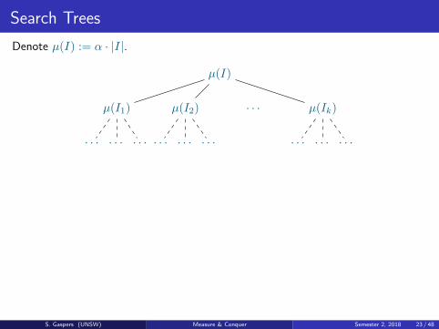
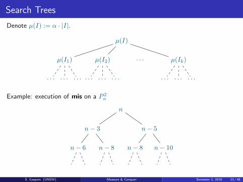
Search Trees
Denote µ(I) := α · |I|.
µ(I)
µ(I1)
. . . . . . . . .
µ(I2)
. . . . . . . . .
. . . µ(Ik)
. . . . . . . . .
Example: execution of mis on a P 2n
n
n− 3
n− 6 n− 8
n− 5
n− 8 n− 10
S. Gaspers (UNSW) Measure & Conquer Semester 2, 2018 23 / 48
Search Trees
Denote µ(I) := α · |I|.
µ(I)
µ(I1)
. . . . . . . . .
µ(I2)
. . . . . . . . .
. . . µ(Ik)
. . . . . . . . .
Example: execution of mis on a P 2n
n
n− 3
n− 6 n− 8
n− 5
n− 8 n− 10
S. Gaspers (UNSW) Measure & Conquer Semester 2, 2018 23 / 48
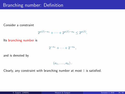
Branching number: Definition
Consider a constraint
2µ(I)−a1 + · · ·+ 2µ(I)−ak ≤ 2µ(I).
Its branching number is
2−a1 + · · ·+ 2−ak ,
and is denoted by
(a1, . . . , ak) .
Clearly, any constraint with branching number at most 1 is satisfied.
S. Gaspers (UNSW) Measure & Conquer Semester 2, 2018 24 / 48
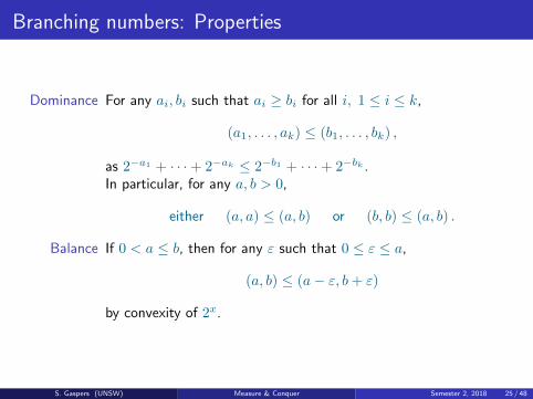
Branching numbers: Properties
Dominance For any ai, bi such that ai ≥ bi for all i, 1 ≤ i ≤ k,
(a1, . . . , ak) ≤ (b1, . . . , bk) ,
as 2−a1 + · · ·+ 2−ak ≤ 2−b1 + · · ·+ 2−bk .In particular, for any a, b > 0,
either (a, a) ≤ (a, b) or (b, b) ≤ (a, b) .
Balance If 0 < a ≤ b, then for any ε such that 0 ≤ ε ≤ a,
(a, b) ≤ (a− ε, b+ ε)
by convexity of 2x.
S. Gaspers (UNSW) Measure & Conquer Semester 2, 2018 25 / 48

Outline
1 Introduction
2 Maximum Independent SetSimple AnalysisSearch Trees and Branching NumbersMeasure & Conquer AnalysisOptimizing the measureExponential Time SubroutinesStructures that arise rarely
3 Further Reading
S. Gaspers (UNSW) Measure & Conquer Semester 2, 2018 26 / 48
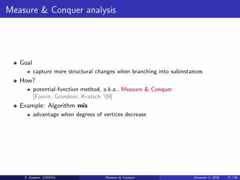
Measure & Conquer analysis
Goal
capture more structural changes when branching into subinstances
How?
potential-function method, a.k.a., Measure & Conquer[Fomin, Grandoni, Kratsch ’09]
Example: Algorithm mis
advantage when degrees of vertices decrease
S. Gaspers (UNSW) Measure & Conquer Semester 2, 2018 27 / 48
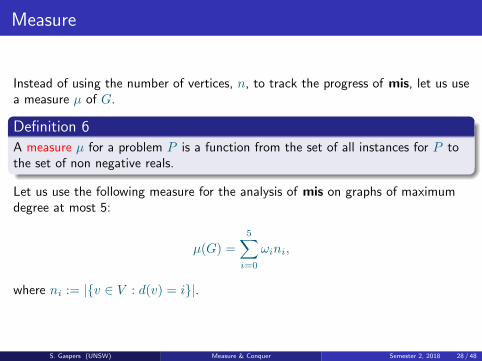
Measure
Instead of using the number of vertices, n, to track the progress of mis, let us usea measure µ of G.
Definition 6A measure µ for a problem P is a function from the set of all instances for P tothe set of non negative reals.
Let us use the following measure for the analysis of mis on graphs of maximumdegree at most 5:
µ(G) =
5∑i=0
ωini,
where ni := |v ∈ V : d(v) = i|.
S. Gaspers (UNSW) Measure & Conquer Semester 2, 2018 28 / 48
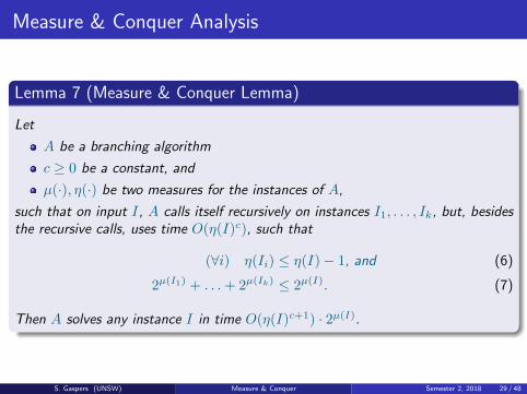
Measure & Conquer Analysis
Lemma 7 (Measure & Conquer Lemma)
Let
A be a branching algorithm
c ≥ 0 be a constant, and
µ(·), η(·) be two measures for the instances of A,
such that on input I, A calls itself recursively on instances I1, . . . , Ik, but, besidesthe recursive calls, uses time O(η(I)c), such that
(∀i) η(Ii) ≤ η(I)− 1, and (6)
2µ(I1) + . . .+ 2µ(Ik) ≤ 2µ(I). (7)
Then A solves any instance I in time O(η(I)c+1) · 2µ(I).
S. Gaspers (UNSW) Measure & Conquer Semester 2, 2018 29 / 48
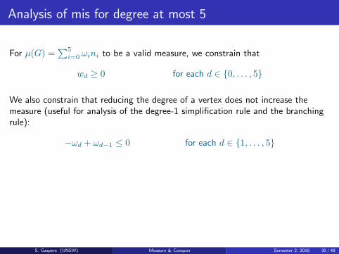
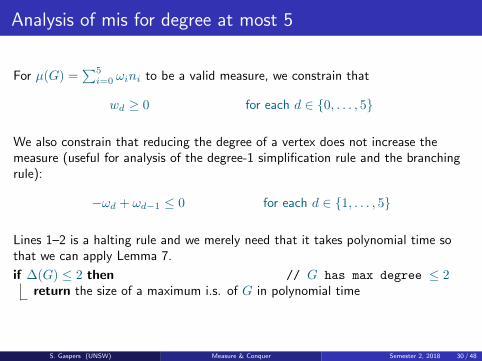
Analysis of mis for degree at most 5
For µ(G) =∑5i=0 ωini to be a valid measure, we constrain that
wd ≥ 0 for each d ∈ 0, . . . , 5
We also constrain that reducing the degree of a vertex does not increase themeasure (useful for analysis of the degree-1 simplification rule and the branchingrule):
−ωd + ωd−1 ≤ 0 for each d ∈ 1, . . . , 5
Lines 1–2 is a halting rule and we merely need that it takes polynomial time sothat we can apply Lemma 7.
if ∆(G) ≤ 2 then // G has max degree ≤ 2return the size of a maximum i.s. of G in polynomial time
S. Gaspers (UNSW) Measure & Conquer Semester 2, 2018 30 / 48
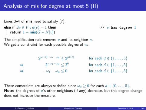
Analysis of mis for degree at most 5 (II)
Lines 3–4 of mis need to satisfy (7).
else if ∃v ∈ V : d(v) = 1 then // v has degree 1return 1 + mis(G−N [v])
The simplification rule removes v and its neighbor u.We get a constraint for each possible degree of u:
2µ(G)−ω1−ωd ≤ 2µ(G) for each d ∈ 1, . . . , 5⇔ 2−ω1−ωd ≤ 20 for each d ∈ 1, . . . , 5⇔ −ω1 − ωd ≤ 0 for each d ∈ 1, . . . , 5
These constraints are always satisfied since ωd ≥ 0 for each d ∈ 0, . . . , 5.Note: the degrees of u’s other neighbors (if any) decrease, but this degree changedoes not increase the measure.
S. Gaspers (UNSW) Measure & Conquer Semester 2, 2018 31 / 48
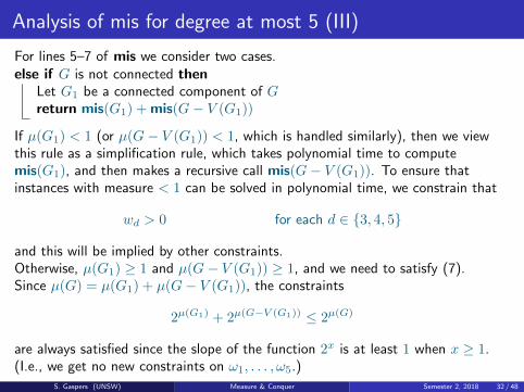
Analysis of mis for degree at most 5 (III)
For lines 5–7 of mis we consider two cases.else if G is not connected then
Let G1 be a connected component of Greturn mis(G1) + mis(G− V (G1))
If µ(G1) < 1 (or µ(G− V (G1)) < 1, which is handled similarly), then we viewthis rule as a simplification rule, which takes polynomial time to computemis(G1), and then makes a recursive call mis(G− V (G1)). To ensure thatinstances with measure < 1 can be solved in polynomial time, we constrain that
wd > 0 for each d ∈ 3, 4, 5
and this will be implied by other constraints.Otherwise, µ(G1) ≥ 1 and µ(G− V (G1)) ≥ 1, and we need to satisfy (7).Since µ(G) = µ(G1) + µ(G− V (G1)), the constraints
2µ(G1) + 2µ(G−V (G1)) ≤ 2µ(G)
are always satisfied since the slope of the function 2x is at least 1 when x ≥ 1.(I.e., we get no new constraints on ω1, . . . , ω5.)
S. Gaspers (UNSW) Measure & Conquer Semester 2, 2018 32 / 48
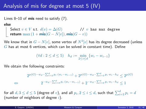
Analysis of mis for degree at most 5 (IV)
Lines 8–10 of mis need to satisfy (7).
elseSelect v ∈ V s.t. d(v) = ∆(G) // v has max degree
return max (1 + mis(G−N [v]),mis(G− v))
We know that in G−N [v], some vertex of N2[v] has its degree decreased (unlessG has at most 6 vertices, which can be solved in constant time). Define
(∀d : 2 ≤ d ≤ 5) hd := min2≤i≤d
wi − wi−1
We obtain the following constraints:
2µ(G)−wd−∑d
i=2 pi·(wi−wi−1) + 2µ(G)−wd−∑d
i=2 pi·wi−hd ≤ 2µ(G)
⇔ 2−wd−∑d
i=2 pi·(wi−wi−1) + 2−wd−∑d
i=2 pi·wi−hd ≤ 1
for all d, 3 ≤ d ≤ 5 (degree of v), and all pi, 2 ≤ i ≤ d, such that∑di=2 pi = d
(number of neighbors of degree i).
S. Gaspers (UNSW) Measure & Conquer Semester 2, 2018 33 / 48
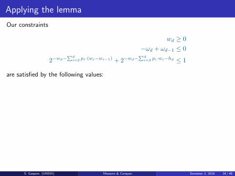
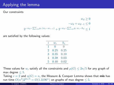
Applying the lemma
Our constraints
wd ≥ 0
−ωd + ωd−1 ≤ 0
2−wd−∑d
i=2 pi·(wi−wi−1) + 2−wd−∑d
i=2 pi·wi−hd ≤ 1
are satisfied by the following values:
i wi hi1 0 02 0.25 0.253 0.35 0.104 0.38 0.035 0.40 0.02
These values for wi satisfy all the constraints and µ(G) ≤ 2n/5 for any graph ofmax degree ≤ 5.Taking c = 2 and η(G) = n, the Measure & Conquer Lemma shows that mis hasrun time O(n3)22n/5 = O(1.3196n) on graphs of max degree ≤ 5.
S. Gaspers (UNSW) Measure & Conquer Semester 2, 2018 34 / 48
Outline
1 Introduction
2 Maximum Independent SetSimple AnalysisSearch Trees and Branching NumbersMeasure & Conquer AnalysisOptimizing the measureExponential Time SubroutinesStructures that arise rarely
3 Further Reading
S. Gaspers (UNSW) Measure & Conquer Semester 2, 2018 35 / 48
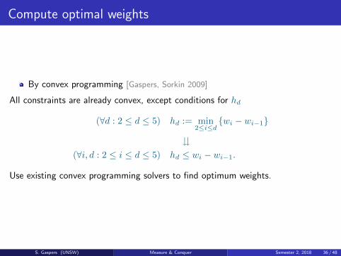
Compute optimal weights
By convex programming [Gaspers, Sorkin 2009]
All constraints are already convex, except conditions for hd
(∀d : 2 ≤ d ≤ 5) hd := min2≤i≤d
wi − wi−1
(∀i, d : 2 ≤ i ≤ d ≤ 5) hd ≤ wi − wi−1.
Use existing convex programming solvers to find optimum weights.
S. Gaspers (UNSW) Measure & Conquer Semester 2, 2018 36 / 48
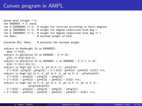
Convex program in AMPL
param maxd integer = 5;set DEGREES := 0..maxd;var W DEGREES >= 0; # weight for vertices according to their degreesvar g DEGREES >= 0; # weight for degree reductions from deg ivar h DEGREES >= 0; # weight for degree reductions from deg <= ivar Wmax; # maximum weight of W[d]
minimize Obj: Wmax; # minimize the maximum weight
subject to MaxWeight d in DEGREES:Wmax >= W[d];
subject to gNotation d in DEGREES : 2 <= d:g[d] <= W[d]-W[d-1];
subject to hNotation d in DEGREES, i in DEGREES : 2 <= i <= d:h[d] <= W[i]-W[i-1];
subject to Deg3 p2 in 0..3, p3 in 0..3 : p2+p3=3:2^(-W[3] -p2*g[2] -p3*g[3]) + 2^(-W[3] -p2*W[2] -p3*W[3] -h[3]) <=1;
subject to Deg4 p2 in 0..4, p3 in 0..4, p4 in 0..4 : p2+p3+p4=4:2^(-W[4] - p2*g[2] - p3*g[3] - p4*g[4])
+ 2^(-W[4] - p2*W[2] - p3*W[3] - p4*W[4] - h[4]) <=1;subject to Deg5 p2 in 0..5, p3 in 0..5, p4 in 0..5, p5 in 0..5 :
p2+p3+p4+p5=5:2^(-W[5] - p2*g[2] - p3*g[3] - p4*g[4] - p5*g[5])
+ 2^(-W[5] - p2*W[2] - p3*W[3] - p4*W[4] - p5*W[5] - h[5]) <=1;
S. Gaspers (UNSW) Measure & Conquer Semester 2, 2018 37 / 48
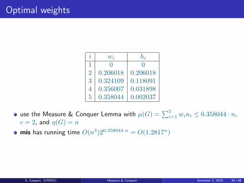
Optimal weights
i wi hi1 0 02 0.206018 0.2060183 0.324109 0.1180914 0.356007 0.0318985 0.358044 0.002037
use the Measure & Conquer Lemma with µ(G) =∑5i=1 wini ≤ 0.358044 · n,
c = 2, and η(G) = n
mis has running time O(n3)20.358044·n = O(1.2817n)
S. Gaspers (UNSW) Measure & Conquer Semester 2, 2018 38 / 48
Outline
1 Introduction
2 Maximum Independent SetSimple AnalysisSearch Trees and Branching NumbersMeasure & Conquer AnalysisOptimizing the measureExponential Time SubroutinesStructures that arise rarely
3 Further Reading
S. Gaspers (UNSW) Measure & Conquer Semester 2, 2018 39 / 48
Exponential time subroutines
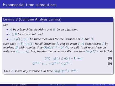
Lemma 8 (Combine Analysis Lemma)
Let
A be a branching algorithm and B be an algorithm,
c ≥ 0 be a constant, and
µ(·), µ′(·), η(·) be three measures for the instances of A and B,
such that µ′(I) ≤ µ(I) for all instances I, and on input I, A either solves I byinvoking B with running time O(η(I)c+1) · 2µ′(I), or calls itself recursively oninstances I1, . . . , Ik, but, besides the recursive calls, uses time O(η(I)c), such that
(∀i) η(Ii) ≤ η(I)− 1, and (8)
2µ(I1) + . . .+ 2µ(Ik) ≤ 2µ(I). (9)
Then A solves any instance I in time O(η(I)c+1) · 2µ(I).
S. Gaspers (UNSW) Measure & Conquer Semester 2, 2018 40 / 48
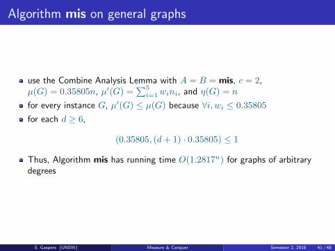
Algorithm mis on general graphs
use the Combine Analysis Lemma with A = B = mis, c = 2,µ(G) = 0.35805n, µ′(G) =
∑5i=1 wini, and η(G) = n
for every instance G, µ′(G) ≤ µ(G) because ∀i, wi ≤ 0.35805
for each d ≥ 6,
(0.35805, (d+ 1) · 0.35805) ≤ 1
Thus, Algorithm mis has running time O(1.2817n) for graphs of arbitrarydegrees
S. Gaspers (UNSW) Measure & Conquer Semester 2, 2018 41 / 48
Outline
1 Introduction
2 Maximum Independent SetSimple AnalysisSearch Trees and Branching NumbersMeasure & Conquer AnalysisOptimizing the measureExponential Time SubroutinesStructures that arise rarely
3 Further Reading
S. Gaspers (UNSW) Measure & Conquer Semester 2, 2018 42 / 48
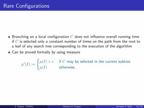
Rare Configurations
Branching on a local configuration C does not influence overall running timeif C is selected only a constant number of times on the path from the root toa leaf of any search tree corresponding to the execution of the algorithm
Can be proved formally by using measure
µ′(I) :=
µ(I) + c if C may be selected in the current subtree
µ(I) otherwise.
S. Gaspers (UNSW) Measure & Conquer Semester 2, 2018 43 / 48
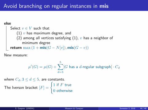
Avoid branching on regular instances in mis
elseSelect v ∈ V such that
(1) v has maximum degree, and(2) among all vertices satisfying (1), v has a neighbor of
minimum degreereturn max (1 + mis(G−N [v]),mis(G− v))
New measure:
µ′(G) = µ(G) +
5∑d=3
[G has a d-regular subgraph] · Cd
where Cd, 3 ≤ d ≤ 5, are constants.
The Iverson bracket [F ] =
1 if F true
0 otherwise
S. Gaspers (UNSW) Measure & Conquer Semester 2, 2018 44 / 48
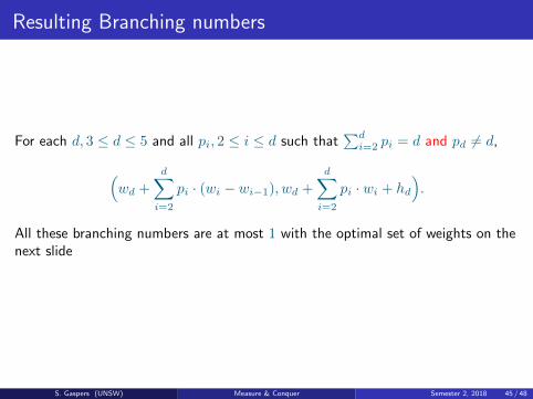
Resulting Branching numbers
For each d, 3 ≤ d ≤ 5 and all pi, 2 ≤ i ≤ d such that∑di=2 pi = d and pd 6= d,
(wd +
d∑i=2
pi · (wi − wi−1), wd +
d∑i=2
pi · wi + hd
).
All these branching numbers are at most 1 with the optimal set of weights on thenext slide
S. Gaspers (UNSW) Measure & Conquer Semester 2, 2018 45 / 48
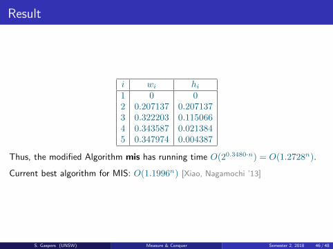
Result
i wi hi1 0 02 0.207137 0.2071373 0.322203 0.1150664 0.343587 0.0213845 0.347974 0.004387
Thus, the modified Algorithm mis has running time O(20.3480·n) = O(1.2728n).
Current best algorithm for MIS: O(1.1996n) [Xiao, Nagamochi ’13]
S. Gaspers (UNSW) Measure & Conquer Semester 2, 2018 46 / 48
Outline
1 Introduction
2 Maximum Independent SetSimple AnalysisSearch Trees and Branching NumbersMeasure & Conquer AnalysisOptimizing the measureExponential Time SubroutinesStructures that arise rarely
3 Further Reading
S. Gaspers (UNSW) Measure & Conquer Semester 2, 2018 47 / 48
Further Reading
Chapter 2, Branching inFedor V. Fomin and Dieter Kratsch. Exact Exponential Algorithms. Springer,2010.
Chapter 6, Measure & Conquer inFedor V. Fomin and Dieter Kratsch. Exact Exponential Algorithms. Springer,2010.
Chapter 2, Branching Algorithms inSerge Gaspers. Exponential Time Algorithms: Structures, Measures, andBounds. VDM Verlag Dr. Mueller, 2010.
S. Gaspers (UNSW) Measure & Conquer Semester 2, 2018 48 / 48