7 אשונ :םוטאה לש ינורטקלאה הנבמה · 7/7/2010 · Robert Andrews Millikan Experiment: Oil Drop, 1909 1868 –1953, USA Nobel Prize in Physics, 1923 Conclusion:

© Prof. Zvi C. Koren1 19.07.10

The Electronic Structure of the Atom:

Historical Background

Fireworks

:7נושא

:המבנה האלקטרוני של האטוםרקע היסטורי

movie


Rutherford

Millikan

Maxwell

Thomson

Einstein

Heisenberg

SchrödingerBohr

Balmer

Planck

Rydberg

de BroglieBorn


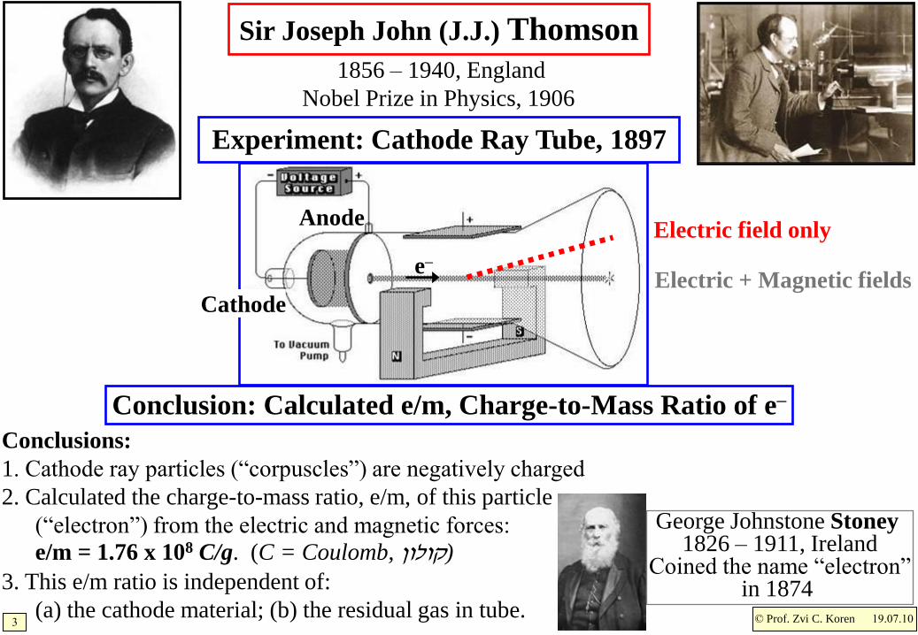
Sir Joseph John (J.J.) Thomson

Conclusions:

1. Cathode ray particles (“corpuscles”) are negatively charged

2. Calculated the charge-to-mass ratio, e/m, of this particle

(“electron”) from the electric and magnetic forces:

e/m = 1.76 x 108 C/g. (C = Coulomb, קולון)

3. This e/m ratio is independent of:

(a) the cathode material; (b) the residual gas in tube.

Experiment: Cathode Ray Tube, 1897

Electric field only

Electric + Magnetic fieldsCathode

Anode

1856 – 1940, England

Nobel Prize in Physics, 1906

George Johnstone Stoney1826 – 1911, Ireland

Coined the name “electron”in 1874

Conclusion: Calculated e/m, Charge-to-Mass Ratio of e–

e–


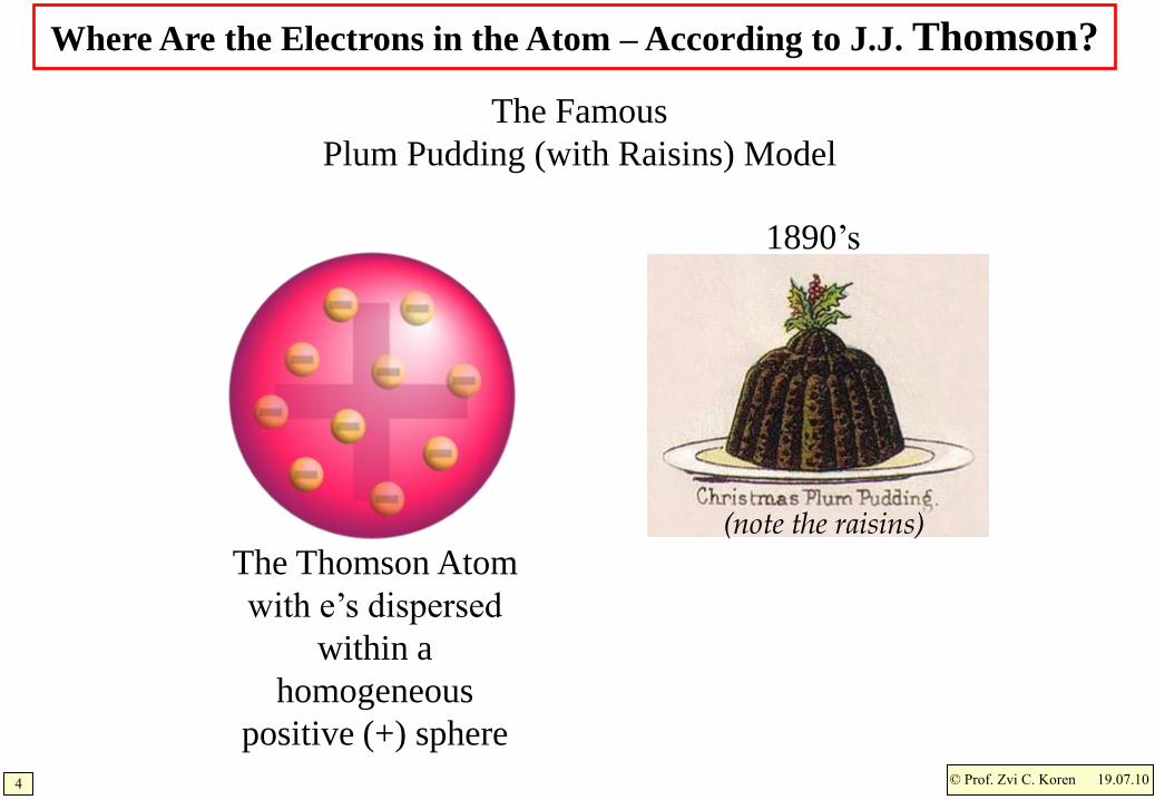
(note the raisins)

Where Are the Electrons in the Atom – According to J.J. Thomson?

The Famous

Plum Pudding (with Raisins) Model

1890’s

The Thomson Atom

with e’s dispersed

within a

homogeneous

positive (+) sphere


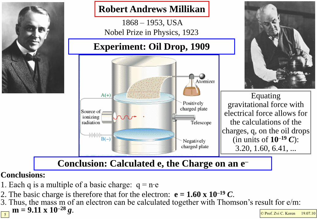
Robert Andrews Millikan

Experiment: Oil Drop, 1909

1868 – 1953, USA


Conclusion: Calculated e, the Charge on an e–

Conclusions:

1. Each q is a multiple of a basic charge: q = n·e

2. The basic charge is therefore that for the electron: e = 1.60 x 10–19 C.3. Thus, the mass m of an electron can be calculated together with Thomson’s result for e/m:

m = 9.11 x 10–28 g.

Equatinggravitational force with

electrical force allows for the calculations of the

charges, q, on the oil drops (in units of 10–19 C):3.20, 1.60, 6.41, ...


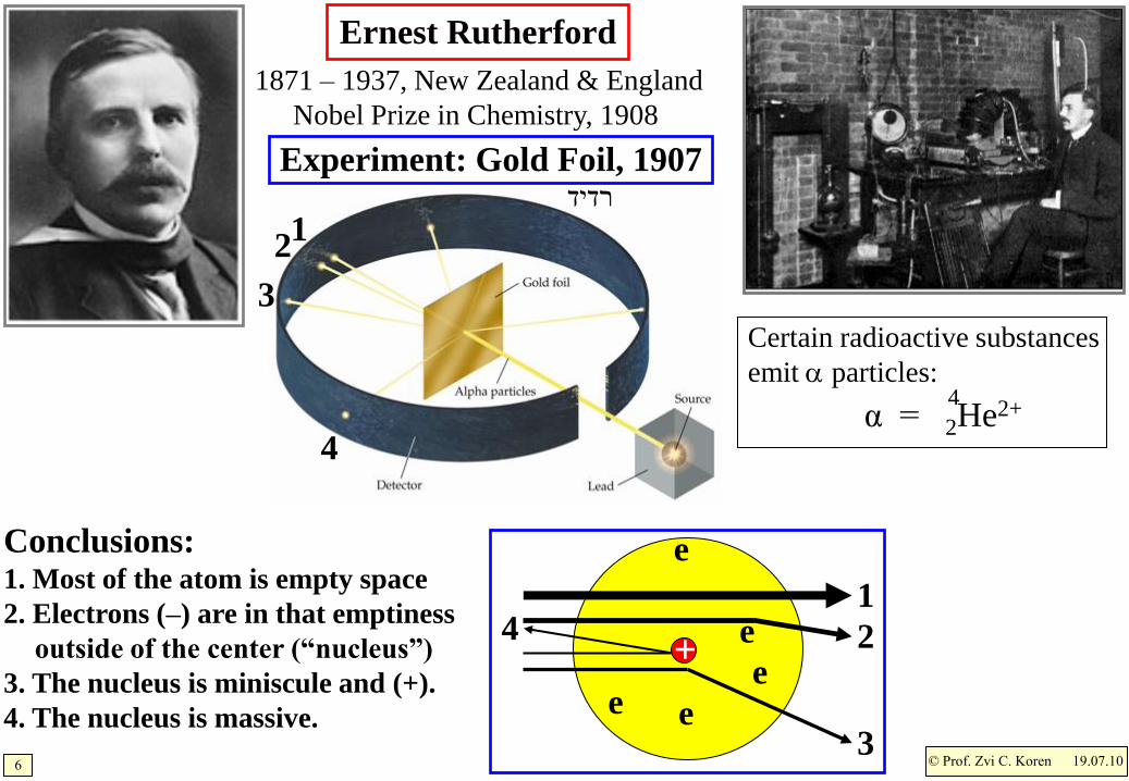
α = 2He2+4

Ernest Rutherford

Experiment: Gold Foil, 1907

1871 – 1937, New Zealand & England

Nobel Prize in Chemistry, 1908

Conclusions:1. Most of the atom is empty space

2. Electrons (–) are in that emptiness

outside of the center (“nucleus”)

3. The nucleus is miniscule and (+).

4. The nucleus is massive.

Certain radioactive substances

emit particles:

12

3

4

+

1

2

3

4

e

e

e

ee

רדיד


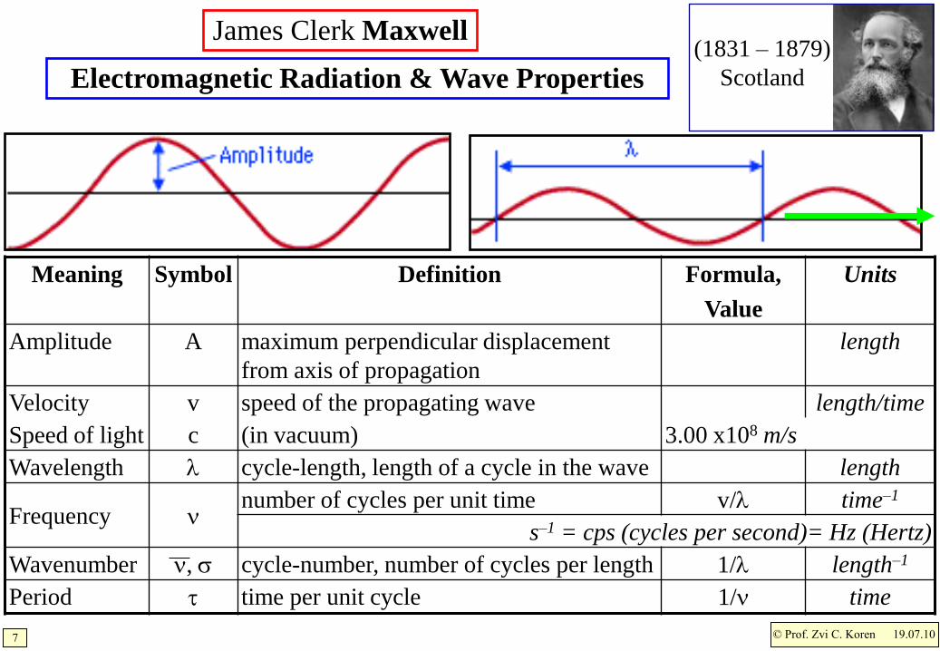
UnitsFormula,

Value

DefinitionSymbolMeaning

lengthmaximum perpendicular displacement

from axis of propagation

AAmplitude

length/timespeed of the propagating wavevVelocity

3.00 x108 m/s(in vacuum)cSpeed of light

lengthcycle-length, length of a cycle in the waveWavelength

time–1v/number of cycles per unit timeFrequency

s–1 = cps (cycles per second)= Hz (Hertz)

length–11/cycle-number, number of cycles per length, Wavenumber

time1/time per unit cycletPeriod

Electromagnetic Radiation & Wave Properties

James Clerk Maxwell(1831 – 1879)

Scotland


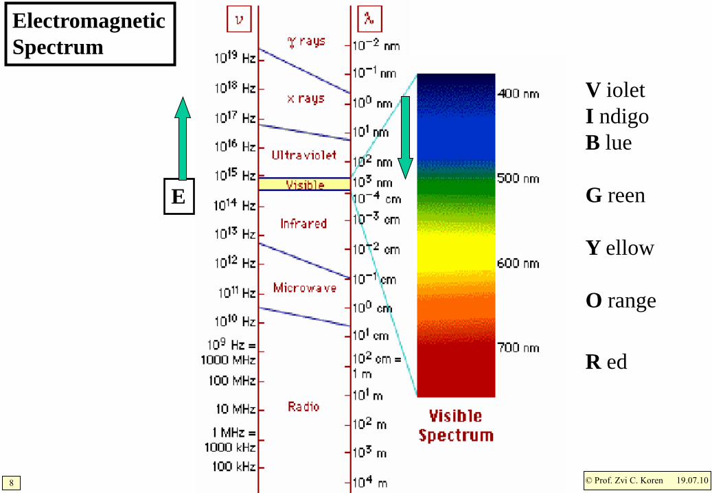
Electromagnetic

Spectrum

E

V iolet

I ndigo

B lue

G reen

Y ellow

O range

R ed


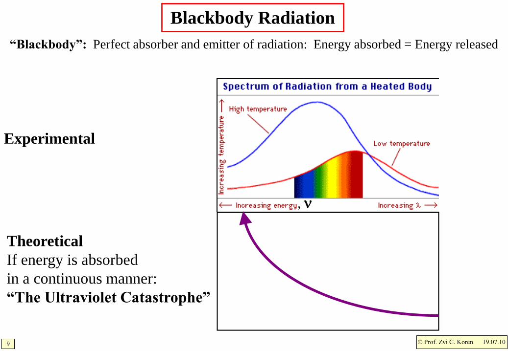
Blackbody Radiation

,

“Blackbody”: Perfect absorber and emitter of radiation: Energy absorbed = Energy released

Experimental

Theoretical

If energy is absorbed

in a continuous manner:

“The Ultraviolet Catastrophe”


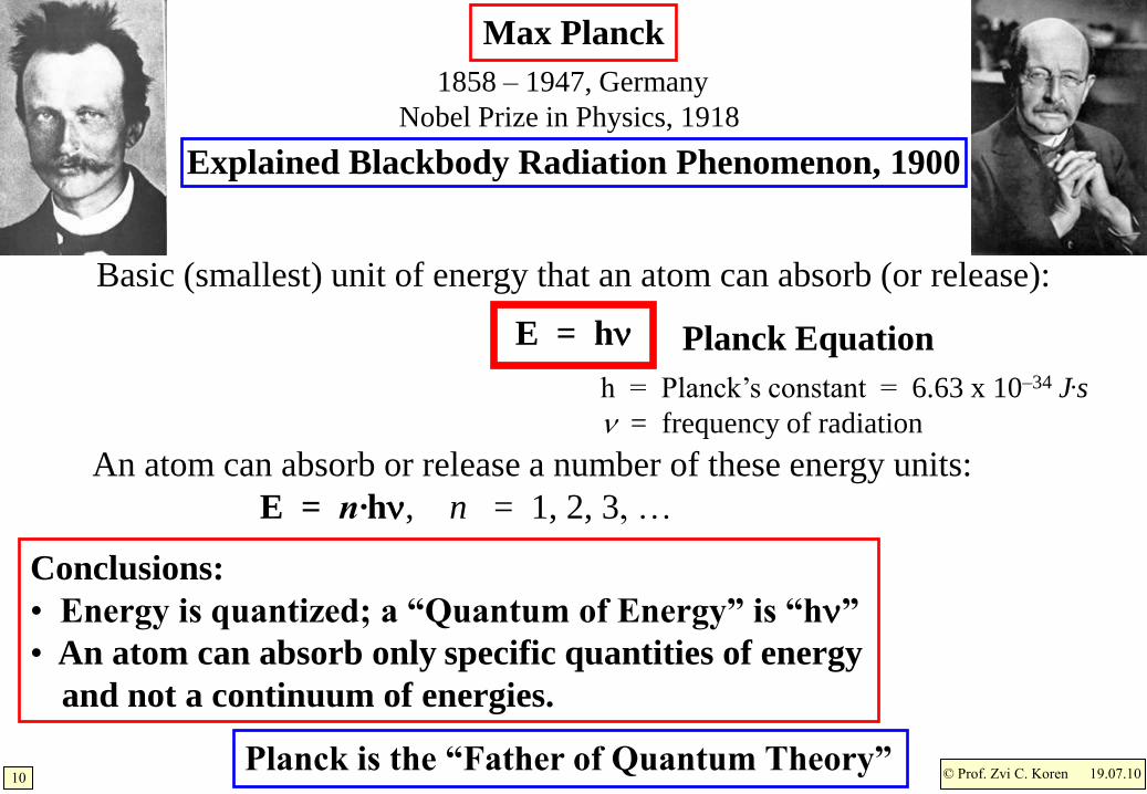
E = h

h = Planck’s constant = 6.63 x 10–34 J.s

= frequency of radiation

Basic (smallest) unit of energy that an atom can absorb (or release):

An atom can absorb or release a number of these energy units:

E = n·h, n = 1, 2, 3, …

Max Planck

Explained Blackbody Radiation Phenomenon, 1900

1858 – 1947, Germany


Conclusions:

• Energy is quantized; a “Quantum of Energy” is “h”

• An atom can absorb only specific quantities of energy

and not a continuum of energies.

Planck Equation

Planck is the “Father of Quantum Theory”


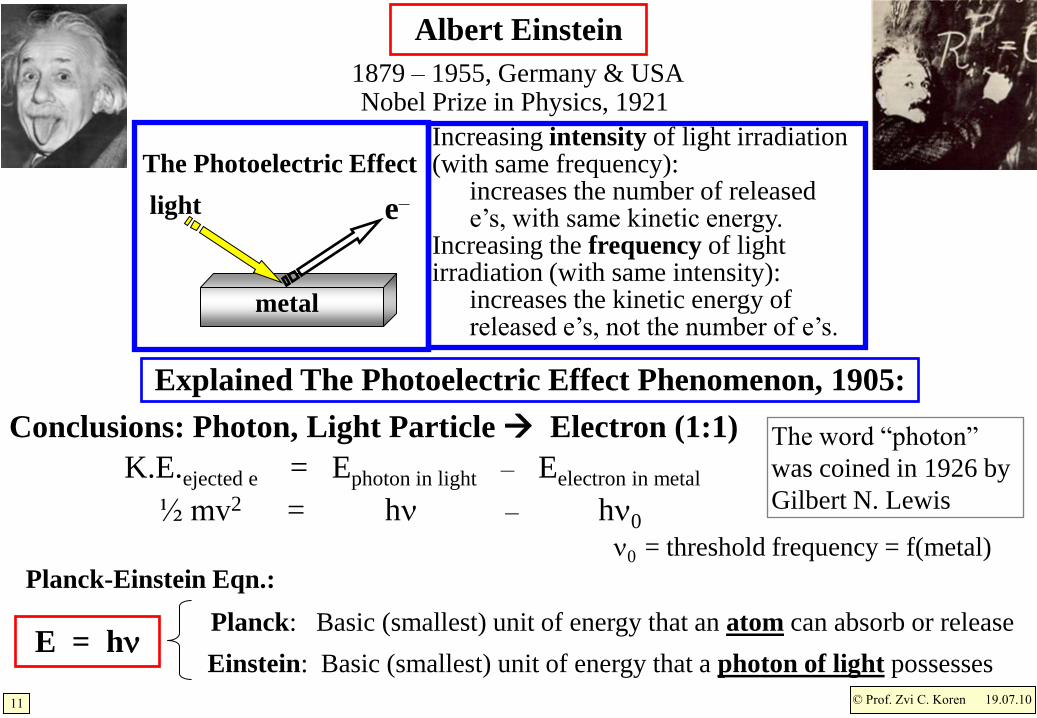
Albert Einstein

K.E.ejected e = Ephoton in light – Eelectron in metal

½ mv2 = h – h0

0 = threshold frequency = f(metal)

E = hPlanck: Basic (smallest) unit of energy that an atom can absorb or release

Einstein: Basic (smallest) unit of energy that a photon of light possesses

Planck-Einstein Eqn.:

e–light

metal

Explained The Photoelectric Effect Phenomenon, 1905:

Increasing intensity of light irradiation (with same frequency):

increases the number of released e’s, with same kinetic energy.

Increasing the frequency of light irradiation (with same intensity):

increases the kinetic energy of released e’s, not the number of e’s.

The Photoelectric Effect

Conclusions: Photon, Light Particle Electron (1:1)

1879 – 1955, Germany & USANobel Prize in Physics, 1921

The word “photon”

was coined in 1926 by

Gilbert N. Lewis


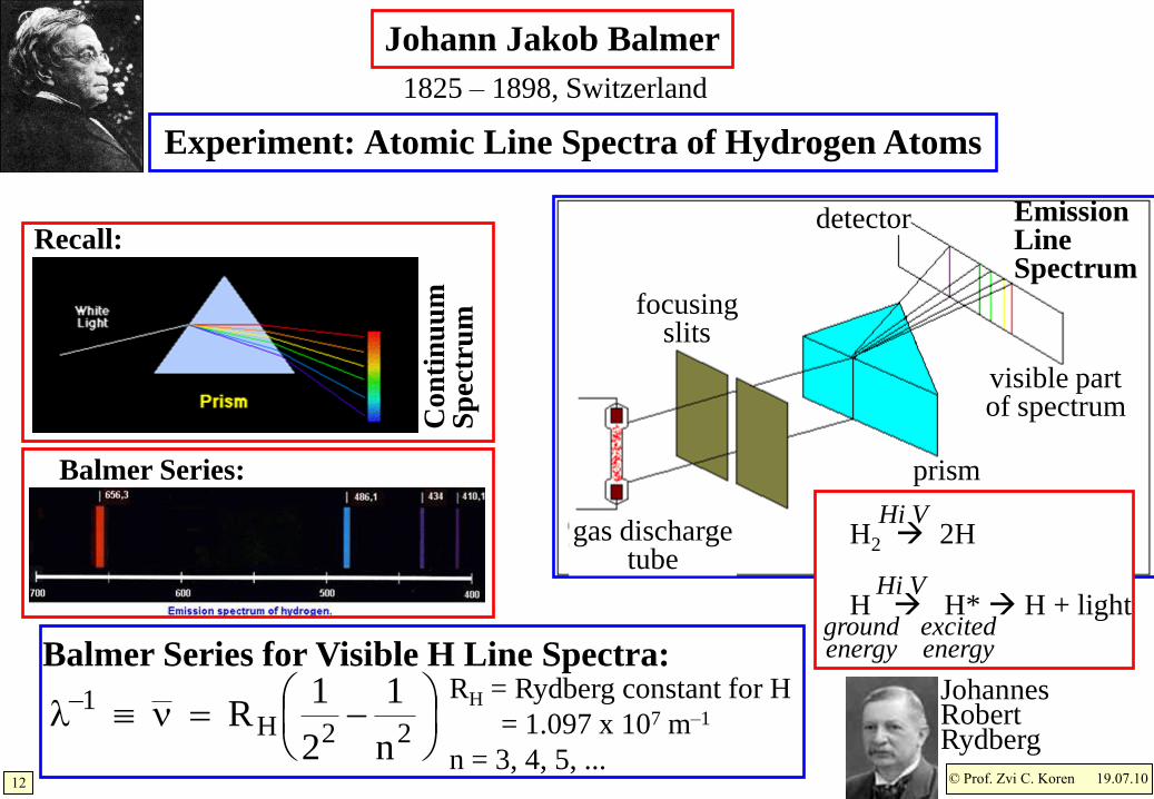
Balmer Series for Visible H Line Spectra:RH = Rydberg constant for H

= 1.097 x 107 m–1

n = 3, 4, 5, ...

Johann Jakob Balmer

Experiment: Atomic Line Spectra of Hydrogen Atoms

1825 – 1898, Switzerland

Co

nti

nu

um

Sp

ectr

um

EmissionLineSpectrum

focusingslits

prism

detector

visible partof spectrum

refraction

gas dischargetube

22H1

n

1

2

1R

prism

whitelight

Recall:

JohannesRobertRydberg

H2 2H

H H* H + light

Hi V

groundenergy

excitedenergy

Hi V

Balmer Series:


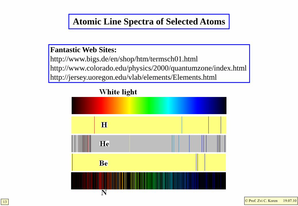
Atomic Line Spectra of Selected Atoms

Fantastic Web Sites:

http://www.bigs.de/en/shop/htm/termsch01.html

http://www.colorado.edu/physics/2000/quantumzone/index.html

http://jersey.uoregon.edu/vlab/elements/Elements.html


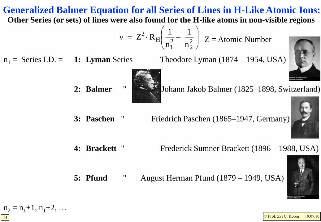
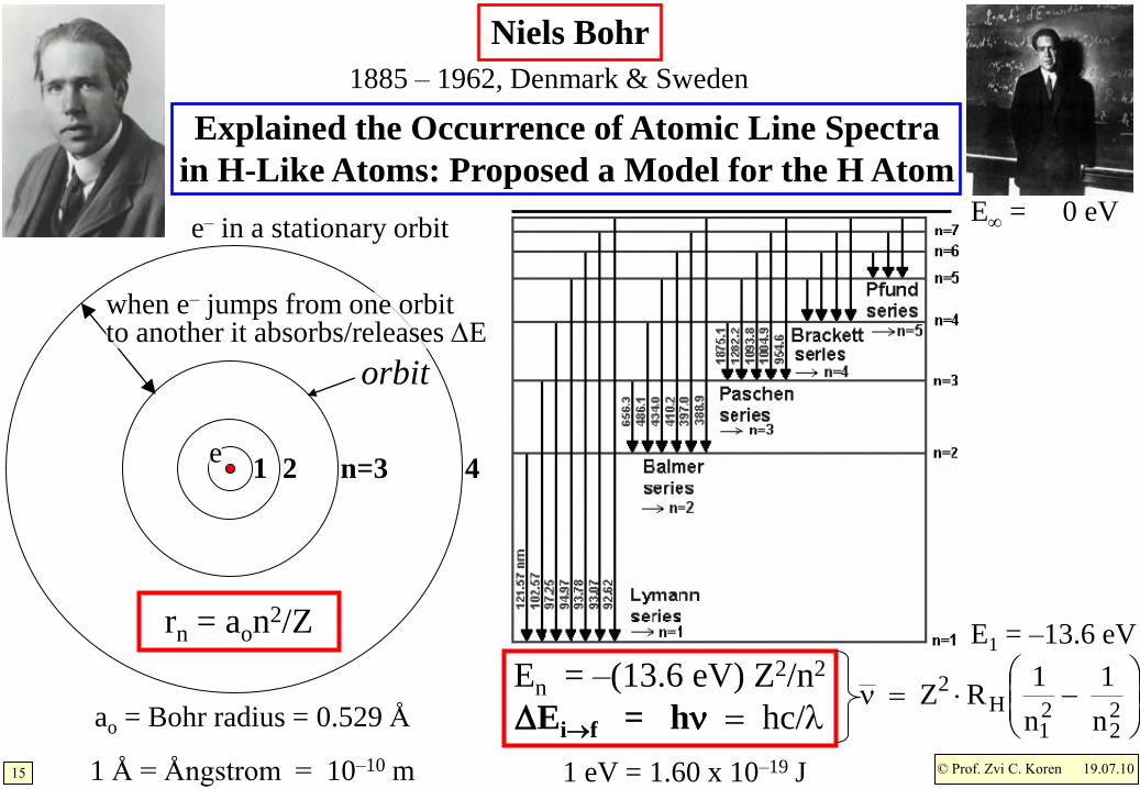
Generalized Balmer Equation for all Series of Lines in H-Like Atomic Ions:

22

21

H2

n

1

n

1R Z

n1 = Series I.D. = 1: Lyman Series Theodore Lyman (1874 – 1954, USA)

2: Balmer " Johann Jakob Balmer (1825–1898, Switzerland)

3: Paschen " Friedrich Paschen (1865–1947, Germany)

4: Brackett " Frederick Sumner Brackett (1896 – 1988, USA)

5: Pfund " August Herman Pfund (1879 – 1949, USA)

n2 = n1+1, n1+2, …

Other Series (or sets) of lines were also found for the H-like atoms in non-visible regions

Z = Atomic Number


rn = aon2/Z

1 Å = Ångstrom = 10–10 m

ao = Bohr radius = 0.529 Å

Niels Bohr

1885 – 1962, Denmark & Sweden

orbit

1 2 n=3 4

Explained the Occurrence of Atomic Line Spectra

in H-Like Atoms: Proposed a Model for the H Atom

E1 = –13.6 eV

e– in a stationary orbit

when e– jumps from one orbitto another it absorbs/releases E

e

22

21

H2

n

1

n

1R Z

En = –(13.6 eV) Z2/n2

Eif = h hc/

E = 0 eV

1 eV = 1.60 x 10–19 J


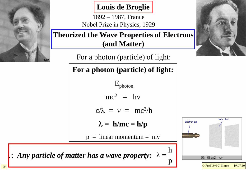
For a photon (particle) of light:

Ephoton

mc2 = h

c/ = = mc2/h

= h/mc = h/p

p = linear momentum = mv

Any particle of matter has a wave property:

Louis de Broglie

1892 – 1987, France


Theorized the Wave Properties of Electrons

(and Matter)

For a photon (particle) of light:

p

h


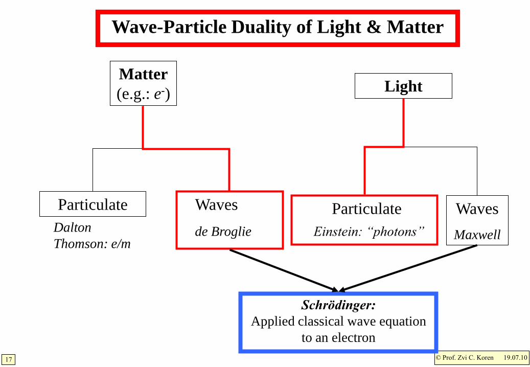
Wave-Particle Duality of Light & Matter

Matter

(e.g.: e-) Light

Particulate

Dalton

Thomson: e/m

Waves

Maxwell

Particulate

Einstein: “photons”

Waves

de Broglie

Schrödinger:

Applied classical wave equation

to an electron


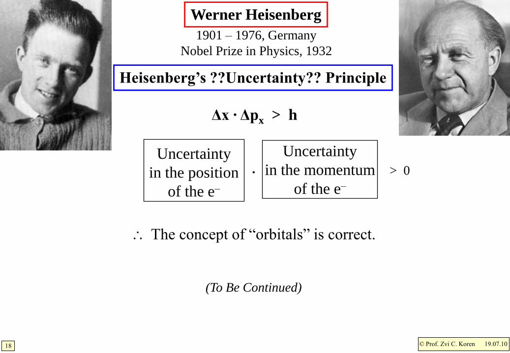
Δx · Δpx > h

Heisenberg’s ??Uncertainty?? Principle

Werner Heisenberg

1901 – 1976, Germany


Uncertainty

in the position

of the e–

Uncertainty

in the momentum

of the e–

> 0·

The concept of “orbitals” is correct.

(To Be Continued)


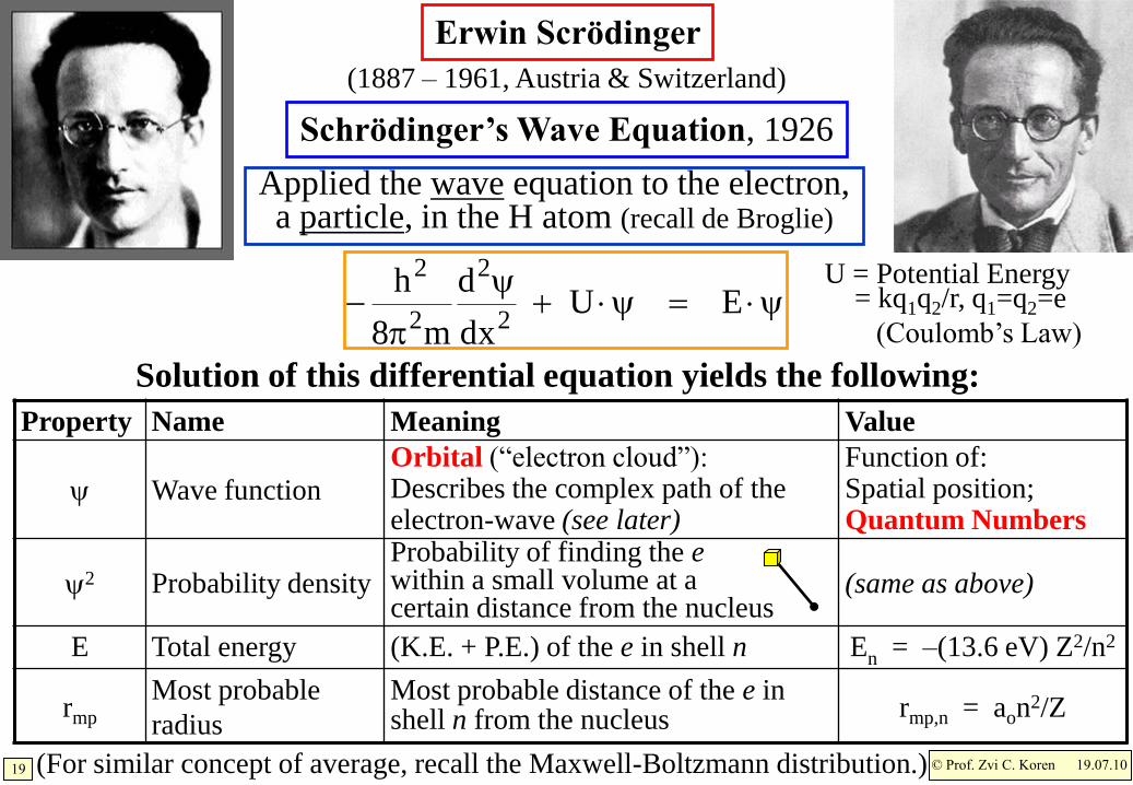
Erwin Scrödinger

(1887 – 1961, Austria & Switzerland)

Schrödinger’s Wave Equation, 1926

E U

dx

d

m8

h2

2

2

2

Applied the wave equation to the electron, a particle, in the H atom (recall de Broglie)

Solution of this differential equation yields the following:

U = Potential Energy= kq1q2/r, q1=q2=e

(Coulomb’s Law)

ValueMeaningNameProperty

Function of:Spatial position;Quantum Numbers

Orbital (“electron cloud”): Describes the complex path of the electron-wave (see later)

Wave function

(same as above)Probability of finding the ewithin a small volume at acertain distance from the nucleus

Probability density2

En = –(13.6 eV) Z2/n2(K.E. + P.E.) of the e in shell nTotal energyE

rmp,n = aon2/Z

Most probable distance of the e in shell n from the nucleus

Most probable

radiusrmp

(For similar concept of average, recall the Maxwell-Boltzmann distribution.)


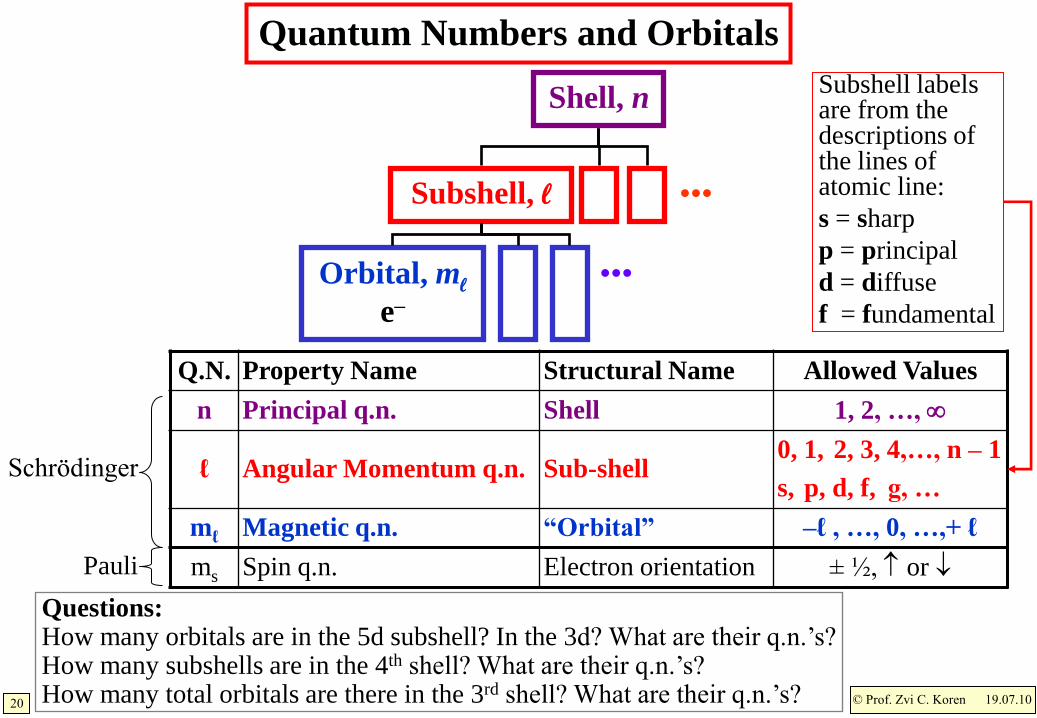
Shell, n

Subshell, ℓ

Orbital, mℓ

e–

Subshell labels are from the descriptions of the lines of atomic line:

s = sharp

p = principal

d = diffuse

f = fundamental

•••

•••

Quantum Numbers and Orbitals

Allowed ValuesStructural NameProperty NameQ.N.

1, 2, …, ShellPrincipal q.n.n

0, 1, 2, 3, 4,…, n – 1

s, p, d, f, g, …Sub-shellAngular Momentum q.n.ℓ

–ℓ , …, 0, …,+ ℓ“Orbital”Magnetic q.n.mℓ

± ½, or Electron orientationSpin q.n.ms

Questions: How many orbitals are in the 5d subshell? In the 3d? What are their q.n.’s?How many subshells are in the 4th shell? What are their q.n.’s?How many total orbitals are there in the 3rd shell? What are their q.n.’s?

Schrödinger

Pauli


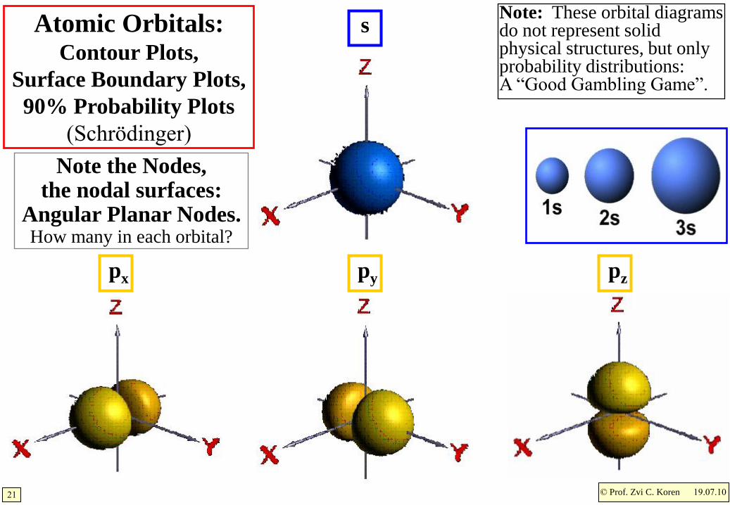
Atomic Orbitals:Contour Plots,

Surface Boundary Plots,

90% Probability Plots

(Schrödinger)

pzpypx

s

Note the Nodes,the nodal surfaces:

Angular Planar Nodes.How many in each orbital?

Note: These orbital diagrams do not represent solid physical structures, but only probability distributions:A “Good Gambling Game”.


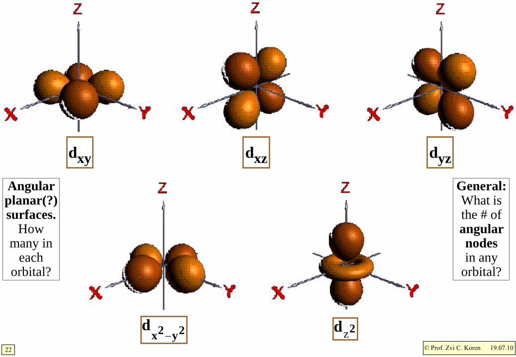
dxy dyz

2y

2x

d

Angular planar(?) surfaces.

How many in

each orbital?

General:What is the # of angular nodesin any

orbital?

2dz

dxz


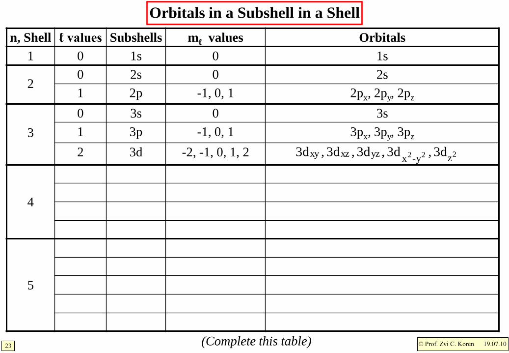
Orbitalsmℓ valuesSubshellsℓ valuesn, Shell

1s01s01

2s02s02

2px, 2py, 2pz-1, 0, 12p1

3s03s0

3 3px, 3py, 3pz-1, 0, 13p1

-2, -1, 0, 1, 23d2

4

5

Orbitals in a Subshell in a Shell

(Complete this table)

222 zy-xyzxzxy 3d ,3d ,3d ,3d ,3d


1s

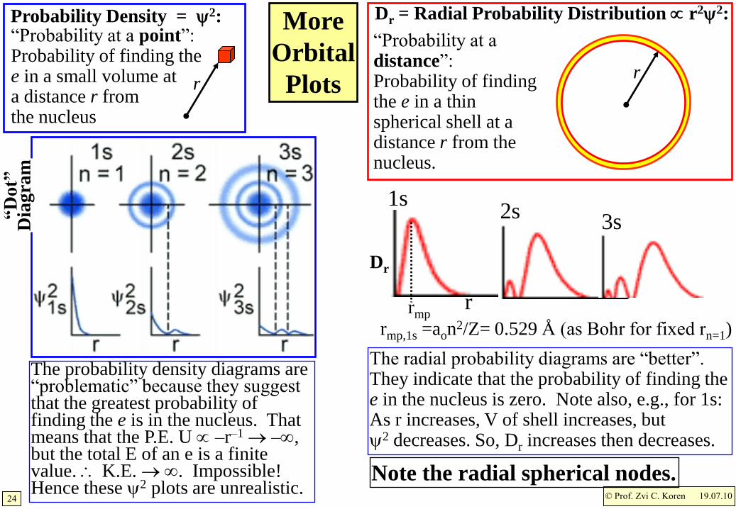
Dr = Radial Probability Distribution r22:

r

“Probability at a point”:Probability of finding the e in a small volume ata distance r fromthe nucleus

The probability density diagrams are “problematic” because they suggest that the greatest probability of finding the e is in the nucleus. That means that the P.E. U –r–1 –, but the total E of an e is a finite value. K.E. . Impossible!Hence these 2 plots are unrealistic.

Probability Density = 2:

The radial probability diagrams are “better”. They indicate that the probability of finding the e in the nucleus is zero. Note also, e.g., for 1s:As r increases, V of shell increases, but2 decreases. So, Dr increases then decreases.

“Probability at a distance”:Probability of finding the e in a thin spherical shell at a distance r from the nucleus.

2s3s

Dr

rrmp

rmp,1s =aon2/Z= 0.529 Å (as Bohr for fixed rn=1)

Note the radial spherical nodes.

More

Orbital

Plots

“D

ot”

Dia

gra

m

r


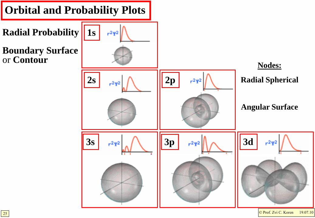
Orbital and Probability Plots

3d3p3s

2p2s

1s

Nodes:

Radial Spherical

Angular Surface

Radial Probability

Boundary Surfaceor Contour


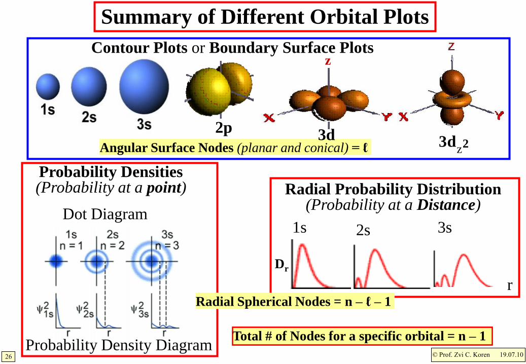
Probability Densities(Probability at a point)

Summary of Different Orbital Plots

1s 2s 3s

Dr

r

Radial Probability Distribution(Probability at a Distance)

Dot Diagram

Angular Surface Nodes (planar and conical) = ℓ

Probability Density Diagram

2p23d

z

Radial Spherical Nodes = n – ℓ – 1

Total # of Nodes for a specific orbital = n – 1

Contour Plots or Boundary Surface Plots

3d

z

Documents

7 אשונ :םוטאה לש ינורטקלאה הנבמה · 7/7/2010 · Robert Andrews Millikan Experiment: Oil Drop, 1909 1868 –1953, USA Nobel Prize in Physics, 1923 Conclusion: