7 Acknowledgments 8 References - bme.ccny.cuny.edubme.ccny.cuny.edu/faculty/lparra/publish/rotorBM.pdf7 Acknowledgments We want to thank ... trated the convergence of learning in some

Continuous Boltzmann Machine with Rotor Neurons June 20, 1994 23

7 Acknowledgments

We want to thank specially Stefan Mießbach for numerous contributions in proving the

convergence properties of the net dynamic and for advice concerning the “cornered rat”

example. We are very grateful to Ingrid Gabler for supplying the experimental data for this

same example.

8 References

D. Ackley, G. Hinton, T. Sejnowski (1985): A Learning Algorithm for BoltzmannMachines. Cognitive SCience 9, 147-169

J.V. Breakwell (1977): Zero-Sum Differential Games with Piece-Wise Continuous Trajec-tories, Lecture Notes of Control and Information Science, 3

R.O. Duda, P.E. Hart (1973): Pattern Classification and Scene Analysis. Wiley - Inter-science

T. Gabler, S. Miesbach, H.M. Breitner, H.J. Pesch (1993): Synthesis of Optimal Strategiesfor Differential Games by Neural Networks. Schwerpunktprogramm der Deutschen Fors-chungsgemeinschaft: Anwendungsbezogene Optimierung und Steuerung, Report No. 468

L. Gislén, C. Peterson, B. Södeberg (1992): Rotor Neurons: Basic Formalism and Dynam-ics, Neural Computation 4, 737-745

Moody, C. Darken (1989): Fast Learning in Network of locally-tuned Processing Units.Neural Computation, 1(2)

Moody, C. Darken (1990): Fast Adaptive K-Means Clustering: Some Empirical Result.Int. Joint Conf. on Neural Networks, San Diego

M.C. Mozer, R.S. Zemel, M. Behrmann, C.K.I. Williams (1992): Learning to SegmentImages Using Dynamic Feature Binding, Neural Computation 4, 650-665

A. Noest (1988): Associative Memory in Sparse Phasor Neural Networks, EurophysicsLetters 6 (6), 469-474

C. Peterson, J. Anderson (1987): A Mean Field Theory Algorithm for Neural Networks,Complex Systems 1, 995-1019

B. Schürmann (1989): Stability and Adaption in Artificial Neural Systems, PhysicalReview A, Vol. 40, No. 5, September 1, 2681-2688

F. Silva, L. Almeida (1990): Speeding up Backpropagation. Advanced Neural Computers,Elsevier Science Publischer B.V. (North-Holland) 151-158


6.3 Convergence of the dynamic

We show now the local convergence of the dynamic defined by the MF equations (21) and

(22).

(48)

We remark that this iterative update algorithm for solving equations (21) and (22) can also

be viewed as discrete time integration of equation (35) with time scale . Beside of

this, under condition of finite temperature and properly bounded connection weights the

local convergence of the algorithm can be shown explicitly. According to the Banach

fixed-point theorem local convergence is guaranteed if

(49)

(50)

The forth rank tensor can be written as (38) substituting V by U and G by F.

Since the corresponding conditions (44) and (47) still hold, the inequalities (39) and (40)

are also valid for this tensor. It is thus positive definite, with positive eigenvalues

(51)

Now we can bound the norm as

(52)

(53)

where 1/d is the maximal slope of F at the zero point. At the end we get from (49) condi-

tion for the local convergence:

(54)

Vi t 1+( ) f1T--- Wij Vj t( )⋅

j∑–

=

∆t 1=

Vjl∂∂fik 1<

Vjl∂∂fik

Unm∂∂fik

Vjl∂∂Unm

nm∑ ∇ Vf

WT-----⋅= =

∇ Vf g≡

λ ik gikik

gjlik

jl ik≠∑+

gikik

gjlik

jl ik≠∑–

[ , ]∈

∇ Vf maxik λ ik maxik gikik

gjlik

jl ik≠∑+

maxik 2gikik

<≤=

2maxikFUi-----

Uik2

Ui2

-------- FUi-----– F'+

+

2maxiFUi----- F

Ui-----– F'+

+ ≤ 2

d---= =

Vjl∂∂fik ∇ Vf

WT-----⋅ ∇ Vf W

T-----

2dT------ W 1< <≤=


This holds because G and G’ are positive for positive arguments. Furthermore, we have to

show that

(40)

The right side can be rewritten as

(41)

Considering (39) and (41) we have to show

, and (42)

(43)

As

(44)

holds, (43) is equivalent to

(45)

Since for any vector holds, it is enough to verify,

(46)

This last holds by definition because

(47)

hikik

hjlik

jl ik≠∑>

VikVilδji

Vi2

------------------- GVi-----– G'+

jl ik≠∑

VikVil

Vi2

-------------- GVi-----– G'+

l k≠∑

Vil

Vi2

--------- GVi-----– G'+ Vil

l k≠∑= =

GVi-----

Vik2

Vi2

------- GVi-----– G'+

–Vik

Vi2

---------- GVi-----– G'+ Vil

l k≠∑– 0>

VikGVi-----– G'+

GVi-----– G'+ Vil

l k≠∑– G

Vi

Vik----------<

GVi-----– G'+ 0<

GVi----- G'– Vil

l∑ G

Vi

Vik----------<

Vk Vll∑ V≤ ≤

GVi----- G'– Vi G<

0 G ′Vi<


6.2 Liapunov function

Now we show some convergence properties of the proposed MF equation following the

same lines as Hopfield. Equations (21) and (22) give obviously the fixed-point of the fol-

lowing partial differential equation,

(35)

To demonstrate that the dynamic converges to this fixed-point we have to show that there

exists some Liapunov function,

(36)

where exists, since everywhere. The path integrals can be

performed over an arbitrary curve since the integrand has zero rotation. In order to verify

that L is a Liapunov function, we have to show that its time derivative is negative:

(37)

The inequality is valid if is positive definite. Note that in (37) the symmetry

of the connection strengths was needed. With the weaker condition of detailed balance the

Liapunov characteristic was proved for the original Hopfield model by Schürmann (89).

To prove that the forth rank tensor is positive definite we use the theorem of Gershgorin.

In order to avoid misunderstanding we use now the complete index notation. We abbrevi-

ate and :

(38)

First we show that the diagonal elements are positive:

(39)

td

dUi U– i1T--- Wij f Uj( )⋅

j∑+=

L1

2T------ Vi Wij Vj⋅ ⋅ f

1–V( ) dV⋅

0

Vi

∫i∑+

ij∑–=

f1–

V V⁄ F1–

V( )= F' 0>

tddL

td

dVi 1T--- Wij Vj⋅ f

1–Vi( )–

j∑

⋅i∑– td

dVi

td

dUi⋅i∑– td

dVi ∇ Vjfi

1–

td

dVj 0<⋅ ⋅ij∑–= = =

∇ Vjf

1–Vi( )

Vi Vi= G F1–

Vi( )=

hjlik

Vjl∂∂fik

1–

δjlik G

Vi-----

VikVilδji

Vi2

------------------- GVi-----– G'+

–=≡

hikik

hikik G

Vi-----

Vik2

Vi2

------- GVi-----– G'+

+GVi----- 1

Vik2

Vi2

-------– Vik

2

Vi2

-------G' 0≥+= =


trated the convergence of learning in some numerical experiments. Specially, we demon-

strated the ability to perform piecewise continuous mappings, which represents a difficult

task for non-recursive networks. The multidimensional extension was found advantageous

compared to 2-dimensional units in the case of mapping into 3-dimensional directions.

6 Appendix

6.1 Saddle-point and MF variables.

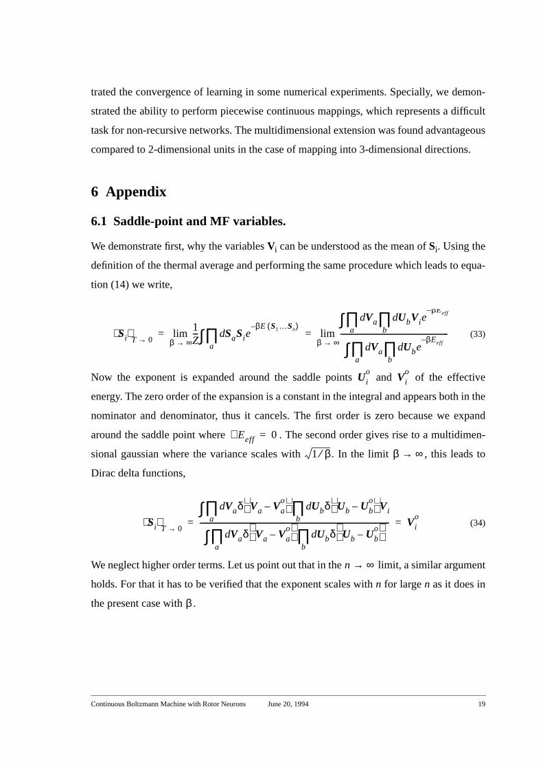
We demonstrate first, why the variables Vi can be understood as the mean of Si. Using the

definition of the thermal average and performing the same procedure which leads to equa-

tion (14) we write,

(33)

Now the exponent is expanded around the saddle points and of the effective

energy. The zero order of the expansion is a constant in the integral and appears both in the

nominator and denominator, thus it cancels. The first order is zero because we expand

around the saddle point where . The second order gives rise to a multidimen-

sional gaussian where the variance scales with . In the limit , this leads to

Dirac delta functions,

(34)

We neglect higher order terms. Let us point out that in the limit, a similar argument

holds. For that it has to be verified that the exponent scales with n for large n as it does in

the present case with .

Si⟨ ⟩T 0→

1Z--- SaSie

βE S1…Sn( )–d

a∏∫β ∞→

lim

Va UbVieβEeff–

db∏d

a∏∫

Va UbeβEeff–

db∏d

a∏∫

-----------------------------------------------------------β ∞→lim= =

Uio

Vio

Eeff∇ 0=

1 β⁄ β ∞→

Si⟨ ⟩T 0→

Vaδ Va Vao

– Ubδ Ub Ub

o–

Vidb∏d

a∏∫

Vaδ Va Vao

– Ubδ Ub Ub

o–

d

b∏d

a∏∫

-------------------------------------------------------------------------------------------------------- Vio

= =

n ∞→

β


number of hidden rotor neurons was selected in order to give the same number of learning

parameters, about 80. In the three dimensional rotor net we used four hidden units and in

the two dimensional we used 5 hidden units. The training and generalization sets con-

tained 100 points each. The error decreased down to about 8.5o and to 15o for the three

and for the two dimensional case respectively. Specially the generalization error differs

considerably (14o and 41o) (see FIGURE 9). This suggests that the 3-dimensional rotors

capture the desired relation much better because the inherent structure fits this problem.

Thus whenever a direction in an n-dimensional (n>2) space is searched, we expect that an

n-dimensional rotor net will solve the mapping task better than any net with 2-dimensional

units.

FIGURE 9 Training and generalization error for a three and a two dimensional rotor net.

5 Conclusion

The purpose of this work was the formulation of a continuous version of the classical BM.

Therefore, we used the Mean Field theory for rotor neurons. We demonstrated analytically

some convergence properties of the resulting rotor dynamic, and derived the appropriate

mean MF learning algorithm in analogy to the original BM. This way, we also expanded

the models of two dimensional (or complex valued) units to arbitrary dimension. We illus-


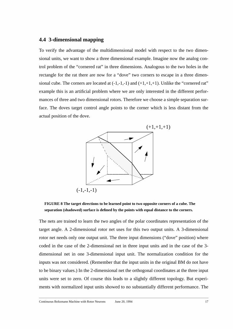
4.4 3-dimensional mapping

To verify the advantage of the multidimensional model with respect to the two dimen-

sional units, we want to show a three dimensional example. Imagine now the analog con-

trol problem of the “cornered rat” in three dimensions. Analogous to the two holes in the

rectangle for the rat there are now for a “dove” two corners to escape in a three dimen-

sional cube. The corners are located at (-1,-1,-1) and (+1,+1,+1). Unlike the “cornered rat”

example this is an artificial problem where we are only interested in the different perfor-

mances of three and two dimensional rotors. Therefore we choose a simple separation sur-

face. The doves target control angle points to the corner which is less distant from the

actual position of the dove.

FIGURE 8 The target directions to be learned point to two opposite corners of a cube. The

separation (shadowed) surface is defined by the points with equal distance to the corners.

The nets are trained to learn the two angles of the polar coordinates representation of the

target angle. A 2-dimensional rotor net uses for this two output units. A 3-dimensional

rotor net needs only one output unit. The three input dimensions (“dove” position) where

coded in the case of the 2-dimensional net in three input units and in the case of the 3-

dimensional net in one 3-dimensional input unit. The normalization condition for the

inputs was not considered. (Remember that the input units in the original BM do not have

to be binary values.) In the 2-dimensional net the orthogonal coordinates at the three input

units were set to zero. Of course this leads to a slightly different topology. But experi-

ments with normalized input units showed to no substantially different performance. The

(-1,-1,-1)

(+1,+1,+1)


FIGURE 6 The remaining average angular error continuous BM is 5.48°.

FIGURE 7 Mapping produced by a MLP with seven hidden neurons after 6000 epochs of learning.

360°

(0,6)

(10,6)

(0,0)

0°

angleerror

360°

(0,6)

(10,6)

(0,0)

0°

angleresult


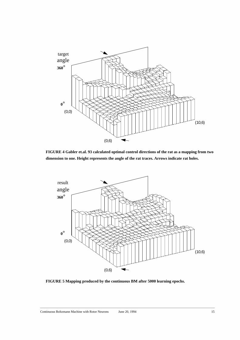
FIGURE 4 Gabler et.al. 93 calculated optimal control directions of the rat as a mapping from two

dimension to one. Height represents the angle of the rat traces. Arrows indicate rat holes.

FIGURE 5 Mapping produced by the continuous BM after 5000 learning epochs.

360°

(0,6)

(10,6)

(0,0)

0°

angletarget

360°

(0,6)

(10,6)

(0,0)

0°

angleresult


“partitioning to one” (Moody, Darken 89) and a linear output. We got the best result of

9.19° average error with eight hidden neurons by initializing the weights with K-means-

clustering and K-nearest-neighbor algorithm following Moody and Darken (90) and Duda

and Hart (73). Comparing FIGURE 5 and FIGURE 7 the difficulty of the MLP to produce

discontinuity can be easily recognized, while the BM reproduced the desired edges quite

well.

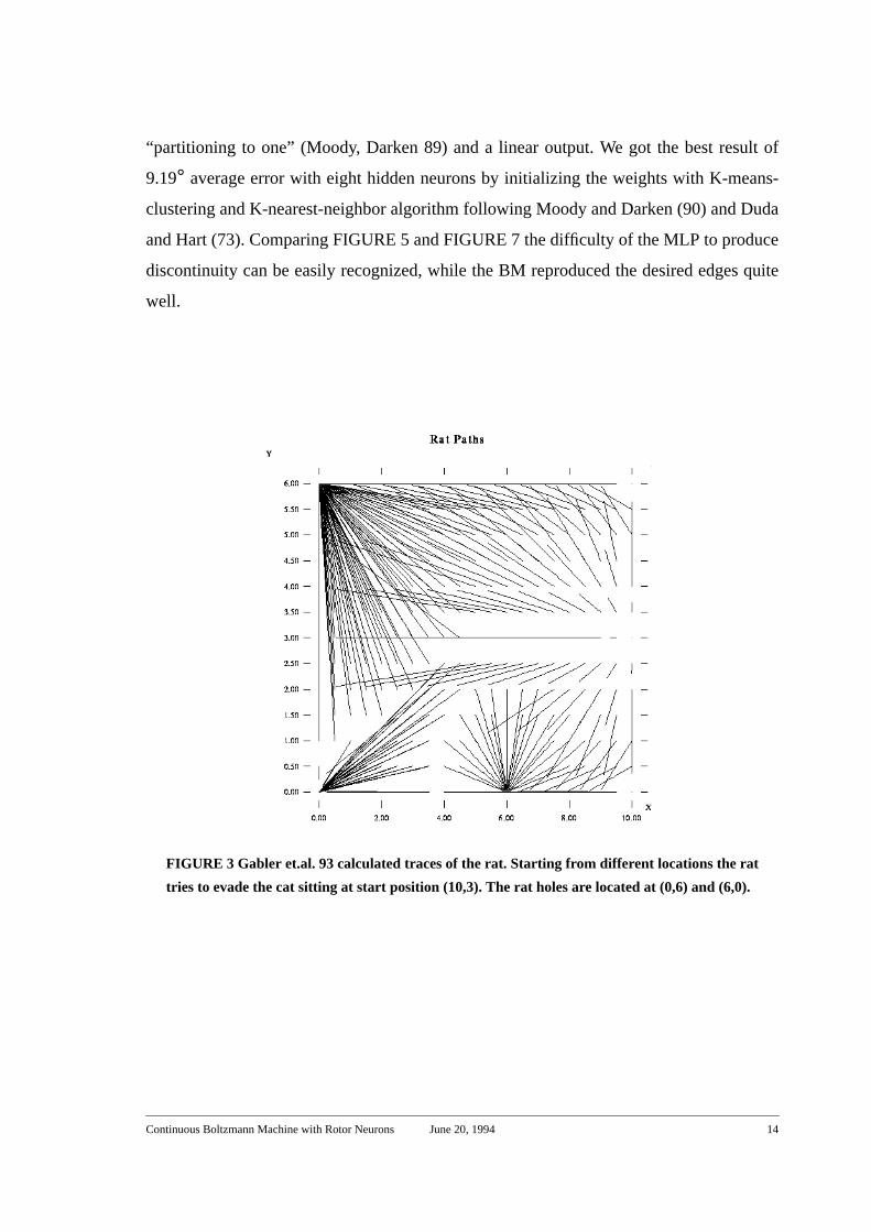
FIGURE 3 Gabler et.al. 93 calculated traces of the rat. Starting from different locations the rat

tries to evade the cat sitting at start position (10,3). The rat holes are located at (0,6) and (6,0).


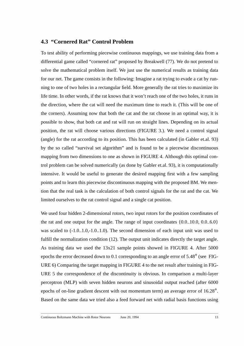
4.3 “Cornered Rat” Control Problem

To test ability of performing piecewise continuous mappings, we use training data from a

differential game called “cornered rat” proposed by Breakwell (77). We do not pretend to

solve the mathematical problem itself. We just use the numerical results as training data

for our net. The game consists in the following: Imagine a rat trying to evade a cat by run-

ning to one of two holes in a rectangular field. More generally the rat tries to maximize its

life time. In other words, if the rat knows that it won’t reach one of the two holes, it runs in

the direction, where the cat will need the maximum time to reach it. (This will be one of

the corners). Assuming now that both the cat and the rat choose in an optimal way, it is

possible to show, that both cat and rat will run on straight lines. Depending on its actual

position, the rat will choose various directions (FIGURE 3.). We need a control signal

(angle) for the rat according to its position. This has been calculated (in Gabler et.al. 93)

by the so called “survival set algorithm” and is found to be a piecewise discontinuous

mapping from two dimensions to one as shown in FIGURE 4. Although this optimal con-

trol problem can be solved numerically (as done by Gabler et.al. 93), it is computationally

intensive. It would be useful to generate the desired mapping first with a few sampling

points and to learn this piecewise discontinuous mapping with the proposed BM. We men-

tion that the real task is the calculation of both control signals for the rat and the cat. We

limited ourselves to the rat control signal and a single cat position.

We used four hidden 2-dimensional rotors, two input rotors for the position coordinates of

the rat and one output for the angle. The range of input coordinates {0.0..10.0, 0.0..6.0}

was scaled to (-1.0..1.0,-1.0..1.0). The second dimension of each input unit was used to

fulfill the normalization condition (12). The output unit indicates directly the target angle.

As training data we used the 13x21 sample points showed in FIGURE 4. After 5000

epochs the error decreased down to 0.1 corresponding to an angle error of 5.48° (see FIG-

URE 6) Comparing the target mapping in FIGURE 4 to the net result after training in FIG-

URE 5 the correspondence of the discontinuity is obvious. In comparison a multi-layer

perceptron (MLP) with seven hidden neurons and sinusoidal output reached (after 6000

epochs of on-line gradient descent with out momentum term) an average error of 16.28°.Based on the same data we tried also a feed forward net with radial basis functions using


input and output unit respectively. The second dimension is used for the normalization condition

(12)

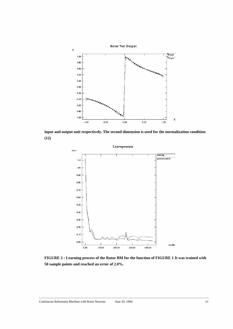
FIGURE 2 : Learning process of the Rotor BM for the function of FIGURE 1 It was trained with

50 sample points and reached an error of 2.0%.


figuration the relaxation will relax always to the same fixed-point. If a small change in the

input occurs, the relaxation point is likely to change also in a small amount, unless the

energy surface is changed by the different input in such a way, that the same starting point

of the relaxation occurs to lay in another basin of attraction. In that case the fixed-point,

towards which the system converges, may differ considerably from the one corresponding

to slightly different input. Thus we expect the system to perform piecewise continuous

mappings. And in fact, in simulations we observe a tendency to perform piecewise contin-

uous mappings. The location of the discontinuity can even be trained, as demonstrated in

the example in FIGURE 1 An arbitrary discontinuous 1-dimensional mapping was trained

(here we used as target function ) The location of the disconti-

nuity is very sensitive with respect to the connection strengths. This explains the peaks of

the learning process in FIGURE 2 In order to compensate for these peaks we used the

learning constant schedule suggested by Silva and Almeida (90). All in all, this kind of

recurrent net has the ability to perform both continuous and discontinuous mappings.

Therefore, we expect good performance especially in piecewise continuous mapping

FIGURE 1 : A Rotor BM with five 2-dimensional units (three hidden, one input and one output

unit) was trained to learn this piecewise continuous map. X and Y denote one dimension of the

f x( ) sig x( ) exp x–( )=


4.1 Coding

We have to use at least a two-dimensional rotor to implement a continuous mapping.

Given the normalization condition (12) for the output and hidden units, we need one

(d+1)-dimensional units to code d-dimensional signals at the output. For any n-dimen-

sional signal one is free to chose between n 2-dimensional unit or a single (n+1)-dimen-

sional rotor. We are free in selecting the sign of the coordinate that is used for the

normalization. We will choose in all our experiments a positive sign. This is of course

arbitrary and makes no difference either to the desired mapping it self, or to the ability of

the net of approximate it. We point out that the formulation of the continuous rotor BM

can be readily rewritten for a combination of rotors with different dimensionality.

We are going to see in paragraph 4.3 that 3-dimensional units are better suited for a map-

ping in the 3-dimensional space, rather than two 2-dimensional units that represent the

two angles of polar coordinates in the 3-dimensional space.

In preliminary experiments we used 2-dimensional units. To verify the learning algorithm

we tested as a discrete mapping the XOR problem. With similar parameters we came to

the same result as in the original work of Peterson (87). Furthermore the capacity of learn-

ing simple continuous mapping like the 1-dimensional sine function has been checked.

The net trained with 20 sample points it and solved the task nearly perfectly (0.9% error).

4.2 Piecewise continuous mapping

We want to explain and demonstrate the inherent ability of the system to perform piece-

wise continuous maps. Discontinuity occurs when small changes in the input values lead

to drastic changes of the output towards which the system relaxes. Remember that since

there exist a Liapunov function for the relaxation at a fixed temperature, the fixed-points

of the Mean Field equations can be understood as the bottoms of the valleys of the energy

function. The fixed-point iteration to calculate these solutions is equivalent to making a

gradient descent on that energy landscape with the step size 1.0. (see Appendix 6.3). The

inputs to the net are kept fixed during the relaxation. They can bee understood as a con-

stant external field, that parameterizes the energy surface. Thus the energy surface

depends continuously on the inputs. Starting with always the same output and hidden con-


(30)

Inserting (28) in (27) and using (29) and (30) we get an analog learning rule

(31)

The bar denotes the average over the desired distribution R, i.e. the average over the learn-

ing patterns. Again with the approximation analog to (11) and equality (17) we write the

MF learning rule,

(32)

Since we are going to apply the continuous BM to the function approximation task, we

will use the obvious modification done by Hopfield (87) where the visible units are further

separated into input and output units. The input units lead to an external field and need not

be restricted to the normalization condition (12). Nevertheless we will be using for sake of

simplicity in some cases normalized inputs.

4 Simulations

The first aim of the simulation was to prove the feasibility of the proposed BM. In some

preliminary experiments we confirmed that the equations (21) and (22) converge for every

temperature in a few update cycles, even with connections which are not symmetric in

. At high temperature the rotor values are moving around the origin of their state space.

While decreasing the temperature the norm of the rotors increases until some freezing

temperature is reached. There and the values remain fixed. We observed in the

experiments that the freezing temperature is correlated with the connection strengths

( is of order one). This gives us a guideline for selecting the temperature

schedule. Starting just above the freezing point we decrease the temperature slowly. In our

experiments we start at temperature 1.0 and decrease it with factor 0.85 until we reach

0.001.

⟨ ⟩ clamped Sihv

P Sihv{ } P Si

v{ }⁄di∏∫ Si

hvP Si

hSi

v{ }di∏∫= =

Wikjl∆ ηβ SikSjl⟨ ⟩ clamped SikSjl⟨ ⟩free

–=

Wikjl∆ ηβ VikVjl( ) clamped VikVjl( )free

–=

k l,

Vi 1≈

W Tfreeze⁄


3.2 Learning rule

We want to expand the derivation of the BM to the multidimensional continuous case.

Basically we have to substitute the trace over the binary state space in the definitions (2),

(3), (5) and (6) by a trace over the continuous space,

(23)

whereby the space of the hidden units, the space of the visible units and the

conjunct space of all units has to be properly considered. This leads to the follow-

ing definitions:

(24)

(25)

(26)

The partition function Z is given by (13). After some calculations we obtain the gradient

of the relative entropy H with respect to the connection strengths,

(27)

(28)

The brackets denote the thermal average defined here as,

(29)

This thermal average is named “free” because the trace is performed over all visible and

hidden units states and there is no constraint on any unit. This is in contrast to the

“clamped” thermal average where the visible units are kept fixed:

∑ Sidi∏∫→

Sih{ } Si

v{ }

Sihv{ }

P Sihv{ } e

βE Sihv{ }–

Z⁄=

P Siv{ } Si

hP Si

hv{ }di∏∫=

H SivR Si

v{ } R Siv{ } P Si

v{ }⁄logdi∏∫=

Wikjl∆ ηWikjl∂∂H

– η SivR Si

v{ } P Siv{ }⁄

Wikjl∂∂

P Siv{ }d

i∏∫= =

Wikjl∂∂

P Siv{ } β Si

hSik

hvSjl

hvP Si

hv{ } SikSjl⟨ ⟩ P Siv{ }–

d

i∏∫=

⟨ ⟩ free Sihv

P Sihv{ }d

i∏∫=


3 Continuous Rotor BM

We use rotors as neurons in the BM to facilitate continuous valued mapping. That way we

get multidimensional units and we have to expand the formulation of the BM to the multi-

dimensional case. We have to define a proper energy function for the relaxation dynamic

and to revise the derivation of the BM learning rule.

3.1 Model description

The structure is analogous to the original BM with rotor neurons. We allow independent

neuron interaction in each direction,

(20)

The indexes enumerate the neurons and the different dimen-

sions in the first notation. The second notation is used to simplify expressions. To guaran-

tee convergence of the dynamics we demand symmetry in and simultaneously in

that is . Equations (18) and (19) now read:

(21)

(22)

This leads to the MF equations for the continuous rotor BM. In one dimension they reduce

to the original MF equation (9) of the discrete BM. Once again, these equations can be

viewed as the fixed-point of the corresponding partial differential equation of first order,

similar to (10). In the appendix we present these continuous time equations and a

Liapunov function that guarantees the convergence to the fixed-point equations (21) and

(22). The convergence of the iterative algorithm that solves this MF equation can be

proved for finite temperatures and bounded connection strength ( ). None-

theless in our simulations the system converges in a few iteration steps whatever connec-

tion strength or temperature we choose, even with not symmetric in .

E12---– SikWikjlSjl

ijkl∑ 1

2---– Si Wij Sj⋅ ⋅

ij∑= =

i j, 1…n= k l, 1…d=

i j, k l,

Wikjl Wjlik=

Ui1T--- Wij Vj⋅

j∑–=

Vi f Ui( )=

2 W Td⁄ 1<

Wikjl k l,


He considers the task of minimizing an energy function . The starting point

for the MF Theory is the so called partition function. The corresponding function for

rotors is defined as

(13)

The integration here is to be performed over the n d-dimensional unit spheres. In order to

realize the desired approximation first introduce new mean field variables Ui and Vi and

evaluate the integrals in Si. The new mean field variables are not restricted to the unit

sphere. That way the state space is replaced by a virtual space. In this virtual

space the states are not restricted anymore to the unit sphere. On these states of course a

different effective potential applies. It appears in the exponent and is different from the

original energy for non zero temperature,

(14)

(15)

G is defined by using the modified Bessel functions Im:

(16)

The variables at the saddle point of the effective potential can be understood as the

mean of Si. In the limit (see Appendix 6.1)

(17)

The saddle points and are given by the following equations:

(18)

(19)

F is the derivative of G and has sigmoid shape. These equations are the corresponding

generalization of the MF equation (9) for the continuous multidimensional case.

E S1…Sn( )

Z

Z eβE S1…Sn( )–

S1… Sndd∫=

Si 1=

Z eβEeff–

V1… Vn U1… Undddd∫∝

Eeff E V1…Vn( ) T Vi Ui T G Ui( )i∑+⋅

i∑–=

G u( ) I d 2–( ) 2⁄ u( )logd 2–

2------------ u( )log–=

Vio

T 0→

Si⟨ ⟩T 0→

Vio

=

Vio

Uio

Uio 1

T--- E V1

o…Vno

Vi∇–=

Vio Ui

o

Uio

---------F Uio

f Ui

0 ≡=


The solution of this equations can be accomplished by iterative updating. In fact, these

equations are the steady state solution of the corresponding partial differential equation of

first order.

(10)

The iterative updating can be regarded as a discrete integration of this equations with time

scale one. For this equation Hopfield gives a Liapunov function that guarantees the con-

vergence of the solution by demanding the connection strengths to be symmetric. A differ-

ent way to derive equations (9) is known as the saddle-point approximation. We will

return to it in the next section. While applying the learning rule (7) one further approxima-

tion is used. The order of correlation and thermal averaging is changed,

(11)

At the end the resulting MF equations give a deterministic algorithm implementing the

basic concept of global search of minimum energy in the recall phase.

2.3 Rotors

There are different approaches to generalizing the Mean Field formalism to continuous

and multidimensional units. Peterson (87) first considered the case of real valued but mul-

tidimensional units called “rotors” for a general energy function. Noest (88) studied the

Hopfield net in the case of imaginary valued elements called “phasors” that were thus

restricted to the two dimensional complex space. Mozer et. al. (92 and related works)

applied phasors in network models including hidden units. We want to generalize the

deterministic discrete BM to the continuous multidimensional case using this time Peter-

son rotors with a quadratic energy function. We also focus on rotors because one may be

interested quite naturally in three or even higher dimensional directional units. Peterson

(87) introduced rotors in a very general manner. They are defined as multidimensional

continuous unit vectors

(12)

tdd

Si⟨ ⟩ Si⟨ ⟩– β wij Sj⟨ ⟩j∑

tanh+=

SiSj⟨ ⟩ Si⟨ ⟩ Sj⟨ ⟩≈

Si ℜ dSi;∈ 1 i; 1…n= =


is used as cost function. In this case it measures the difference between some desired prob-

ability distribution and the actual distribution of the visible units

(5)

Here the probability distribution of the visible units irrespective of the state of the hid-

den units is given by

(6)

The resulting learning rule

(7)

involves only the mean values of the correlation of the state variables. The first term is the

thermal mean value averaged over all presented patterns while keeping the visible units

clamped. The second term is the thermal mean of the completely free running system.

These two expressions can be understood as a Hebb and an anti-Hebb term. But calculat-

ing the accurate thermal average is even more time consuming than reaching the equilib-

rium distribution, so here the mean field approximation comes into consideration.

2.2 Mean Field Approximation

The aim of the MF approximation is to replace the time consuming stochastic procedure

by a deterministic algorithm to calculate the desired mean values. There are different ways

of deriving the corresponding equations. In the MF approximation itself, it is assumed that

(8)

That way one arrives at a set of equations for the mean values of the state variables,

(9)

Rv Pv

H Rv

Rv

Pv-----log

v∑=

h

Pv Pvhh∑=

wij∆ ηwij∂∂H

– ηβ SiSj⟨ ⟩ clamped SiSj⟨ ⟩free

–= =

β wijSjj∑

tanh⟨ ⟩ β wij Sj⟨ ⟩j∑

tanh≈

Si⟨ ⟩ β wij Sj⟨ ⟩j∑

tanh=


(3)

where Z is the partition function of the system and is the inverse temperature.

The index expresses that the sum is to be performed over the entire state space. To

guarantee a Boltzmann distribution of the state variables one should insist on the principle

of detailed balance for the transition probabilities from a state to a

different state . In fact this principle is satisfied by the so called Glauber dynamic

(4)

Here we want to mention that in order to write this expression in this simple form the sym-

metry of the connection strengths has been used. The system is updated many times

according to equation (4) until it converges to a stationary distribution. That is one reason

why the non-deterministic version of the BM is considered to be very slow.

2.1.1 Annealing

The most interesting mathematical property of the Boltzmann distribution is that at low

temperatures it favors the states with low energy. Independent of the initial conditions and

the path, the system is very likely to be found at the low energy states. In the limit of zero

temperature the probability to be in the global minimum is one. The obstacle is that at low

temperature the stationary distribution is reached very slowly in comparison to high tem-

peratures.Therefore it is common to use the annealing procedure, starting at a high tem-

perature and decreasing it with some appropriate temperature schedule.

2.1.2 Boltzmann learning

The basic idea of the BM is to introduce constraints by keeping some of the visible units

fixed and letting the rest of the system relax to a state of low energy. The learning process

should find the proper energy function where the patterns to be learned are represented by

the most probable states at low temperature. In other words the learning should adapt the

connections wij to give the visible units some desired probability distribution. In contrast

to the Hopfield model, the system may use some internal representation of the visible pat-

terns in the hidden units. The learning rule is a gradient descent method. The cross entropy

Z e βEvh–

vh∑=

β 1 T⁄=

vh

W vh v ′h ′→( ) vh

v ′h ′

W Si S– i→( ) 12--- 1 Si β wijSj

j∑

tanh– =


by a fast deterministic algorithm (Peterson, Anderson 87). For the remaining continuity

problem we present a solution using a generalization of the Spin MF theory to continuous

multidimensional elements, which are commonly called “rotors” (Gislén, Peterson, Söde-

berg, 92). Similar units called phasors were presented and studied by Noest (88). These

elements were complex valued and thus restricted to the two dimensions of the complex

space and used in a Hopfield-like net structure without hidden elements. Similarly to this

approach with complex valued connection strengths, Mozer (92) included also two dimen-

sional hidden neurons. We present in this paper the multidimensional generalization of

this model. The units we are going to use are called rotors because they can take values on

a multidimensional unit sphere. They naturally will be suited for cyclic problems or prob-

lems where directions in two, three or more dimensions come in.

In chapter 2 we introduce the classic BM and rotor neurons. We present our multidimen-

sional continuous model in chapter 3. In chapter 4 we report, among other simulations,

results on piecewise continuous mappings. More detailed calculations on the convergence

properties of the model we left for the appendix in chapter 6.

2 Underlying Theory

2.1 The classic BM

The BM consists of binary stochastic units . They may be con-

nected together with symmetric connection strengths wij=wji. The units are divided into

visible and hidden units. The hidden units have no connection to the outside world. The

visible units sometimes are further separated into input and output units. We label the pos-

sible states of the hidden and visible units by and respectively. We use the same

energy function as in the original Hopfield model,

(1)

The name “Boltzmann Machine” comes from the fact that the stationary distribution of

state variables should be given by the Boltzmann-Gibbs distribution,

(2)

Si 1– 1{ , } i,∈ 1…n=

h v

Evh12--- WijSi

vhSj

vh

ij∑–=

Pvh e βEvh– Z⁄=


Continuous Boltzmann Machine with RotorNeurons

Lucas Parra(*) and Gustavo Deco

Siemens AG, Corporate Research and Development, Munich, Germany

(*) Also at the Ludwig-Maximilian-Universität, Institut for Medical Optics,

Munich, Germany.

Request for reprints: Gustavo Deco, Siemens AG, ZFE ST SN 41, Otto-Hahn-Ring 6,

81730 München, Germany.

Phone: +49 89 63647373

Abstract: We define a new network structure to realize a continuous

version of the Boltzmann Machine (BM). Based on Mean Field (MF)

theory for continuous and multidimensional elements named “rotors”

(Gislén, Peterson, and Södeberg, 92) we derive the corresponding MF

learning algorithm. Simulations demonstrate the learning capability of this

network for continuous and piecewise continuous mappings. The rotor

neurons are specially suited for cyclic problems of arbitrary dimension.

1 Introduction

The classical BM is a well known approach to stochastic neural networks (Ackley, Hinton,

and Sejnowski, 85) . It has been designed to generalize the original recurrent Hopfield

model to a system with hidden units, which can build an internal representation of the

desired mapping task. It has been used mainly for pattern completion, encoding problems

etc. The classic BM suffers from two basic disadvantages. First, it is only able to carry out

binary mappings because the model is based on binary spin states; second, the learning

process is very time-consuming because each single learn step requires the calculation of

the mean values of the stochastic state variables. Thus one has to evaluate the trace over

the entire state space, or to perform some Monte Carlo Simulation. This second disadvan-

tage is reduced by the MF theory, where the stochastic annealing process is approximated

Documents

7 Acknowledgments 8 References - bme.ccny.cuny.edubme.ccny.cuny.edu/faculty/lparra/publish/rotorBM.pdf7 Acknowledgments We want to thank ... trated the convergence of learning in some