7 Composite Systems

7 Composite Systems

We turn now to composite systems, and begin by providing the necessary mathematical tools.We then generalise the postulates and discuss the special case of measurements on subsystemsin detail. The consequences of entanglement will become clear in this discussion. We willdemonstrate a conjuring trick which cannot be explained by classical physics. The unitarydynamics can once again be formulated with the aid of Liouville operators. The action ofsimple quantum gates on multiple qubit systems will be introduced.

7.1 Subsystems

We are accustomed from classical physics to the fact that composite systems (or compoundsystems) can be decomposed into their subsystems and that conversely, individual systemscan be combined to give overall composite systems. The classical total system is completelydescribable in terms of the states of its subsystems and their mutual dynamic interactions. Thesolar system with the sun, the planets and the gravitational field is an example. In quantumphysics, however, it is found that composite systems can have in addition completely differentand surprisingly unified properties. These come to light when the composite quantum systemsare in entangled states In such cases, it is indeed true in a certain sense that “the whole ismore than the sum of its parts”. We will present the details in a similar fashion as in Sect. 1.2and begin with a discussion of preparation and measurements.

But first: what are composite systems? There are particular quantum systems whichexhibit an internal structure. One can distinguish in them two or more subsystems whichcan be accessed separately. With this we mean that subsystems can be experimentallyidentified on which individually (and in this sense locally) interventions can be carried out.The corresponding operations are referred to as local operations These can be for examplepreparations or measurements.

We list some bipartite systems consisting of two subsystems. One can prepare quantumsystems for which, in a measurement at two different locations, a photon can be registered ateach location. There are analogous systems involving electrons. There are systems in which atone location a photon and at another an atom are detected. Subsystems are in general termedlocal, but they need not in fact be spatially separated. A composite system can be composedof e. g. an orbit (an external degree of freedom) and the polarisation (an internal degree of

Entangled Systems: New Directions in Quantum Physics. Jürgen AudretschCopyright c© 2007 WILEY-VCH Verlag GmbH & Co. KGaA, WeinheimISBN: 978-3-527-40684-5

116 7 Composite Systems

freedom) of a single quantum object. Of course two separate systems, which are completelyindependent of one another, can also be considered formally as a total system.

It is essential not to assume e. g. for a 2-photon system that the photons involved are them-selves distinguishable (which they are not, as is well-known). The locations at which forexample the photon polarisation is measured are distinguishable. We know that in measure-ments on this system, always exactly two photons are prepared together and therefore theoverall system is a bipartite system. The corresponding subsystems SA and SB are in thiscase associated with the locations of the detectors, A and B (a photon at the location A ora photon at the location B). In general, apparatus which carry out operations are classicalobjects and thus have an individual identity. In contrast, owing to the indistinguishability ofthe photons, the question of which photon was detected in a particular measurement, e.g. bythe detector at the location A, makes no sense. We will return to this point in Sect. 7.9.

Alice and Bob In order to make it especially clear that measurements or manipulations arecarried out on different subsystems SA and SB of the composite system SAB , one often in-troduces the experimentalists Alice and Bob, who carry out local operations on the subsystemSA or SB (often, but not necessarily, at different locations). By referring to Alice and Bob,we emphasize once more that many quantum-mechanical statements are to be understood op-erationally (i. e. as instructions for carrying out an action); e.g. of the type: “If Alice does thisto subsystem SA, then Bob will measure that on subsystem SB”.

Existence We will once again assume, in agreement with the standard interpretation fromSect. 1.2, that such subsystems are not just abstract auxiliary constructions like the quantumsystems in the minimal interpretation, but rather that they exist in reality. With this, we do notmean to imply that a state can be ascribed to an individual subsystem which is independentof the state of the other subsystem. In entangled systems, precisely this independence doesnot exist. This is the cause of many startling quantum-physical effects. It is furthermorenot meant by our assumption of existence in reality that similar elementary particles of thesame type, such as two photons, have individual identities and are therefore distinguishable.The assumption that the photons exist cannot lead us to such conclusions. The possibility ofseparate manipulations, and not the individuality of quantum objects, defines the subsystem(compare Sect. 7.9).

7.2 The Product Hilbert Space

We first wish to supply the mathematical formalism which we need to formulate the physicsof composite systems. We require for this purpose the product Hilbert space.

7.2.1 Vectors

The tensor product HAB of two Hilbert spaces HA and HB , whose dimensions need not bethe same,

HAB = HA ⊗HB (7.1)

7.2 The Product Hilbert Space 117

is itself a Hilbert space. We call HA and HB the factor spaces. For each pair of vectors|ϕA〉 ∈ HA and |χB〉 ∈ HB , there is a product vector in HAB , which can be written indifferent ways

|ϕA〉 ⊗ |χB〉 =: |ϕA〉|χB〉 =: |ϕA, χB〉 =: |ϕ, χ〉 . (7.2)

It is linear in each argument with respect to multiplication by complex numbers.With λ, µ ∈ C

|ϕA〉 ⊗ (λ|χB1 〉+ µ|χB2 〉) = λ|ϕA〉 ⊗ |χB1 〉+ µ|ϕA〉 ⊗ |χB2 〉 , (7.3)

and

(λ|ϕA1 〉+ µ|ϕA2 〉)⊗ |χB〉 = λ|ϕA1 〉 ⊗ |χB〉+ µ|ϕA2 〉 ⊗ |χB〉 . (7.4)

Entangled vectors If |nA〉 is a basis ofHA and |iB〉 is a basis ofHB , then

|nA〉 ⊗ |iB〉 (7.5)

is a basis of HAB . For the dimension of HAB , we have dimHAB = (dimHA)·(dimHB).Every vector |ψAB〉 inHAB can be expanded in terms of the basis

|ψAB〉 =∑

n,i

αni|nA, iB〉 . (7.6)

All the definitions and statements can be directly applied to the product of a finite number ofHilbert spacesHAB...M = HA ⊗HB ⊗ · · · ⊗ HM . We introduce also the abbreviations:

H⊗n := H⊗H⊗ · · ·H, |φ〉⊗n := |φ〉|φ〉 · · · |φ〉 . (7.7)

Vectors in HAB which are not product vectors are called entangled. They can be writtenonly as a superposition of product vectors. We will represent entangled pure states with suchvectors; they will play an important role in the following sections. The superposition is animportant reason for this. It can usually not be read directly off the decomposition in terms ofthe basis (7.6) whether or not a vector |ψAB〉 is entangled. Later, we will develop a criterion(Sect. 8.3.1) and also extend the concept of entanglement to density operators (Sect. 8.1.1).

The scalar product The bra vector of the product vector |ϕA〉 ⊗ |χB〉 has the form

(|ϕA〉 ⊗ |χB〉)† = 〈ϕA| ⊗ 〈χB| =: 〈ϕA|〈χB| =: 〈ϕA, χB| =: 〈ϕ, χ| . (7.8)

It follows from this for the dual corresponding vector of |ψAB〉 as in Eq. (7.6)

〈ψAB| =∑

n,i

α∗ni〈nA, iB | . (7.9)

The scalar product is formed in a “space by space” manner:

〈ϕA, χB|ξA, ζB〉 = 〈ϕA|ξA〉〈χB|ζB〉 . (7.10)

A basis |nA, iB〉 ofHAB is orthonormal if

〈nA, iB|n′A, i′B〉 = δnn′δii′ (7.11)

holds, i. e. when |nA〉 and |iB〉 are an ONB.


The Bell basis As can readily be verified, the following four vectors make up a particularONB in the spaceHAB = HA2 ⊗HB2 of 2-qubit vectors:

|ΦAB± 〉 :=1√2(|0A, 0B〉 ± |1A, 1B〉) , |ΨAB

± 〉 :=1√2(|0A, 1B〉 ± |1A, 0B〉) . (7.12)

This basis plays a special role in many investigations. We shall show later that thesefrequently-used Bell states are maximally entangled. With reference to an implementationin terms of spin polarisation states, |ΨAB

− 〉 is often called a singlet state.

7.2.2 Operators

Product operators Let CA be a linear operator on the space HA and DB a linear operatoronHB . The tensor product

CA ⊗DB =: CADB (7.13)

refers to a product operator, which acts “space by space”,

[CA ⊗DB ]|ϕA, χB〉 = |CAϕA, DBχB〉 . (7.14)

The product operator is a linear operator onHAB

[CA ⊗DB ]∑

n,i

αni|nA, iB〉 =∑

n,i

αni|CAnA, DBiB〉 . (7.15)

The dyadic operator |ψAB〉〈θAB| formed from the product vectors |ψAB〉 = |ϕA, χB〉and |θAB〉 = |ξA, ζB〉 is likewise a product operator

|ψAB〉〈θAB| = |ϕA, χB〉〈ξA, ζB| = (|ϕA〉〈ξA|)⊗ (|χB〉〈ζB|) . (7.16)

The round brackets can also be left off. The identity operator on HAB can be dyadicallyexpanded in terms of an ONB:

1AB =∑

n,i

|nA, iB〉〈nA, iB | = 1A ⊗ 1B . (7.17)

With the identity operator of a factor space, product operators can be constructed whichare particularly important for the physical applications. The extended operators (subsystemoperators) which are indicated by a symbol with a hat

CA := CAB := CA ⊗ 1B; DB := DAB := 1A ⊗DB (7.18)

are defined withinHAB = HA⊗HB , but they act only in the individual factor Hilbert spacesin a nontrivial way. They are also called local operators. CAB and DAB commute withinHAB and they obey the relations

CABDAB = DABCAB = CA ⊗DB . (7.19)

7.2 The Product Hilbert Space 119

Generalised operators Referring to the dyadic decomposition (7.17) of 1AB , we can writethe generalised operator ZAB onHAB in the form

ZAB = 1ABZAB1AB =∑

n,m

∑

i,j

〈nA, iB|ZAB|mA, jB〉(|nA〉〈mA|⊗|iB〉〈jB|) . (7.20)

It is determined by its matrix elements in the orthonormal basis (7.5).

The trace and partial trace The trace is also defined in the usual way in terms of an or-thonormal basis ofHAB

tr[ZAB] := trAB [ZAB] :=∑

n,i

〈nA, iB|ZAB |nA, iB〉 . (7.21)

For product operators, it follows from this that

trAB[CA ⊗DB] =∑

n,i

CAnnDBii = trA[CA] trB [CB] (7.22)

with the matrix elements CAnn and DBii . The trace is constituted “space by space”.

The computation of the partial trace over one of the factor spaces, for example the spaceHA, is particularly important for physical results. It is defined by

trA[ZAB ] :=∑

n

〈nA|ZAB |nA〉 . (7.23)

We can read off from Eq. (7.20) that an operator on HB is generated in the process. Forproduct operators, it follows that

trA[CA ⊗DB] = trA[CA]DB . (7.24)

The overall trace is found to be a series of partial traces

trAB[ZAB] = trB [trA[ZAB ]] = trA[trB[ZAB ]] . (7.25)

Here, the order in which the partial traces are taken is irrelevant.

The operator basis This concept also, which we have already encountered in Sect. 1.2, canbe directly applied to the product spaceHAB . If QAα , α = 1, . . . , (dimHA)2 represents anoperator basis of HA and RBκ , κ = 1, . . . , (dimHB)2 an operator basis of HB , then theproduct operators

TABακ := QAα ⊗ RBκ (7.26)

form an orthonormal basis of the product spaceHAB , owing to

trAB[TAB†ακ TABβλ ] = δαβδκλ . (7.27)


Every operator ZAB , which acts withinHAB , can be expanded in terms of this basis:

ZAB =∑

α,κ

TABακ trAB[TAB†ακ ZAB] . (7.28)

There are operators onHAB which cannot be written as products of two operators in the formCA ⊗DB (cf. Sect. 7.8). But all the operators on HAB can be written as the sum of productoperators.

The product Liouville space We apply the concepts from Sect. 1.2 and form the productLiouville space

LAB = LA ⊗ LB . (7.29)

Its elements are the operators

CAB =∑

α,β

cαβQAα ⊗RBβ (7.30)

on HAB . The Liouville operator is defined through a generalisation of Eq. (1.87) with theHamiltonian HAB onHAB:

LABZAB := LAB(ZAB) :=1[HAB , ZAB]− . (7.31)

7.3 The Fundamentals of the Physics of CompositeQuantum Systems

7.3.1 Postulates for Composite Systems and Outlook

We consider a composite quantum system, which itself is assumed to be isolated. There-fore, we can take over all the postulates from Chaps. 2 and 4 directly. In particular, the stateof the composite system is described by a density operator in a Hilbert space. The oper-ational interpretation of the concept “state” of a quantum system as “the system has beengenerated by a particular preparation procedure” holds here as well. The composite systemSAB... is supposed to consist of subsystems SA, SB, . . .. Since we wish to consider subsys-tems which are themselves quantum systems, it suggests itself that we associate each of themwith a particular Hilbert space HA,HB, . . . Then the only open question is what structurehas the Hilbert space of the composite system, i.e. how is it composed from the HA,HB, . . ..Here, there are in principle many mathematical possibilities. One is for example the directsum HAB... = HA ⊕ HB ⊕ . . .. However, one in fact postulates the tensor product as de-scribed in Sect. 7.2.1, in order to obtain agreement with experiments. This specification hasfar-reaching consequences for all physical statements about composite quantum systems. Weshall be interested in precisely these statements in the following sections.

7.3 The Fundamentals of the Physics of Composite Quantum Systems 121

The postulate The states of an isolated composite system SAB... which is composed of thesubsystems SA, SB, . . . are described by density operators ρAB... in the product Hilbert space

HAB... = HA ⊗HB ⊗ . . . (7.32)

The postulates for isolated systems from Sect. 2.1 and Sect. 4.2 can be applied to the overallsystem SAB.... If a system is not isolated, it can be made into an isolated system by includingthe “rest of the world”. It then becomes itself a subsystem.

Outlook We can immediately read off a series of special properties of composite systemsfrom this postulate. The mathematical product structure (7.32) defines an organisation scheme.We demonstrate it using the example of a bipartite system SAB .

(i) States: a pure state can be a product state |ψAB〉 = |φA〉 ⊗ |χB〉 or an entangled state|ψAB〉 = |φA〉⊗ |χB〉 (compare Sect. 7.2.1). The unusual properties of entangled states,in particular the appearance of non-classical correlations and their applications, will bediscussed in the rest of this chapter and in all the remaining chapters in detail. We con-sider correlated density operators ρAB = ρA ⊗ ρB in Sect. 8.1.

(ii) Observables: there is a special case of the extended observable operators, such asCAB = CA ⊗ 1B , which is generated from an observable operator which acts ononly one of the product spaces. These describe local measurements which are car-ried out on only one of the subsystems (e. g. a measurement of the observable CA onthe subsystem SA). There are however more general Hermitian operators on HAB(e.g. ZAB = CA ⊗ DB + EA ⊗ FB), which cannot be expressed as extended oper-ators. They also correspond to projective measurements of physical observables ZAB .These latter observables are called non-local observables or collective observables. Thecorresponding measurements are non-local measurements, which in general cannot becarried out directly as local measurements on SA and SB . This holds also for thespecial case of the observables which correspond mathematically to operator products(e. g. ZAB = CA ⊗DB), but cannot be implemented physically as local measurementsof the extended observables (CA⊗1B and 1A⊗DB). Non-local measurements are im-portant in connection with quantum correlations and non-local information storage. Wewill therefore discuss them only in Sect. 9.2.

(iii) Unitary evolution: the unitary evolutions also need not have the structure UAB =UA ⊗ UB . There can be for example an interaction between the systems SA and SB .We discuss this in Sect. 7.6. Non-local unitary evolution can act to entangle and to dis-entangle states. In order for a composite system to be in an entangled state, dynamicinteractions between the subsystems must not exist at the same time.

(iv) The postulate (7.32) provides the required possibility of separate interventions and there-fore the resolution of the composite system into subsystems. Not only local observableoperators, but rather all local operators which act on a subsystem commute with all thelocal operators which act on some other subsystem (cf. Eq. (7.19)). This does not de-pend on the order in which the corresponding actions occur. Thus, in measurements on


subsystems, the correlations between the measured values obtained become an impor-tant quantity. They are characterised by the joint probabilities for the occurrence of themeasured values.

7.3.2 The State of a Subsystem, the Reduced Density Operator, andGeneral Mixtures

Via the postulate, the details of the projective measurement of an observable of the compositesystems are determined. This measurement on the composite system is described by an Her-mitian operator onHAB.... The measurement of an observable on a subsystem, e. g. on SA, isincluded as a special case. It is associated with an observable operator CA which acts onHA.This local measurement corresponds inHAB... to a local observable

CAB...E = CA ⊗ 1B ⊗ . . .⊗ 1E . (7.33)

In this chapter, we shall restrict ourselves to composite systems which are composed of twosubsystems. The extension to a greater number of subsystems is straightforward.

Probability statements According to the postulate, the rules for the measurement dynamicsapply also to the states ρAB of the composite system SAB . We investigate the resulting con-sequences for local measurements. To this end, it is expedient to associate to each subsystema reduced density operator by taking the partial trace over the other subsystem

ρA := trB[ρAB

], ρB := trA

[ρAB

]. (7.34)

Since ρAB is a density operator, ρA and ρB likewise fulfill the conditions for being densityoperators. The eigenvalue equation of the observable CA,

CA|c(r)An 〉 = cn|c(r)An 〉, r = 1, . . . , gn (7.35)

leads to the ONB |c(r)An 〉 of HA and the eigenvalues cn with the degeneracies gn. Theprobability of obtaining the measured value cn from a measurement of C on the system SA isthen given by the local projection operator

PAn = PAn ⊗ 1B, PAn :=gn∑

r=1

|c(r)An 〉〈c(r)An | (7.36)

through the mean value

p(cn) = trAB [PAn ρAB] = trA[trBPAn ρAB] = trA[PAn ρ

A] . (7.37)

In a similar manner, for the expectation value of the observables C, we obtain

〈CA〉 = trAB[ρABCA] = trA[ρACA] . (7.38)

To summarise, we can conclude that: all probability statements about local measurements on asubsystem SA are obtained by associating the reduced density operator ρA from Eq. (7.34) tothe system SA and applying the rules postulated for the density operators of isolated systems.

7.3 The Fundamentals of the Physics of Composite Quantum Systems 123

The state of a subsystem Since all probability statements for measurements on SA areunambiguously determined by the reduced density operator ρA, it is tempting to say that thesubsystem SA is in the state ρA. Thus, in Chap. 2, we introduced the concept of a state. Thecomposite system SAB passes through a preparation procedure which leads to the state ρAB .Together with it, the state ρA = trB

[ρAB

]is prepared.

General mixtures If the composite system SAB is in the product state |αAk , βBk 〉, then thesubsystem SA is in the pure state |αAk 〉. If the state of SAB is, in particular, a statistical mixture(blend or proper mixture) of such product states (cf. Chap. 4),

ρAB =∑

s

ps|αAs , βBs 〉〈αAs , βBs | =∑

s

ps|αAs 〉〈αAs |⊗|βBs 〉〈βBs |,∑

s

ps = 1 , (7.39)

then SA or SB are likewise statistical mixtures

ρA = trB [ρAB] =∑

s

ps|αAs 〉〈αAs | , ρB =∑

s

ps|βBs 〉〈βBs | (7.40)

of the states |αAk 〉 or |βBS 〉. They were produced by the preparation procedure and are presentas real states. An ignorance interpretation (compare Sect. 4.3) is possible. Equation (7.40) isobtained from (7.24) and the dyadic decomposition of 1A or 1B .

In general, the state of a quantum systems SAB will not be a statistical mixture as inEq. (7.39). The state of the subsystem SA is then also not a statistical mixture. An ignoranceinterpretation is not possible. Nevertheless, the state is described by a reduced density oper-ator ρA. We therefore employ the concept mixture to this state ρA of SA also, although – asalready mentioned in Sect. 4.2 – no “mixing” has occurred; and we simply leave off the ad-jective “statistical” for clarity. In this case, one also speaks of the state as an improper mixturein contrast to a proper mixture. “Mixture” is thus the umbrella term.

To make this clear, we can consider for example a system SAB which is in a Bell state. Inthis case, the states of the subsystems are maximally mixed as a result of the entanglement

ρA = trB [ΦAB± ] =121A , ρA = trB[ΨAB

± ] =121A . (7.41)

A corresponding relation holds for SB . However, SAB was prepared in a pure state.In quantum systems, the states of subsystems can be mixtures which – with respect to their

preparation – are not statistical mixtures and therefore do not permit an ignorance interpreta-tion. For their density operators, there are formally arbitrarily many ensemble decompositions.There are therefore arbitrarily many statistical mixtures of an isolated individual system, withwhich they can be indistinguishably simulated with respect to all probability statements forlocal measurements. By means of local measurements, one cannot determine whether a den-sity operator ρA belongs to an individual system SA or is rather a reduced density operatorof a subsystem SA which is part of a larger system. This again justifies the application of theterm “mixture” to all reduced density operators. We mention finally that mixtures in classicalphysics are always statistical mixtures. We shall return to the connection with entanglementlater in Sect. 8.1.


7.4 Manipulations on a Subsystem

7.4.1 Relative States and Local Unitary Transformations

Relative states Making use of the ONB |cAn 〉 and |dBi 〉 ofHA orHB , we can write thepure state |ψAB〉 of the composite system SAB as a decomposition

|ψAB〉 =∑

n,i

αni|cAn , dBi 〉 (7.42)

in terms of the basis vectors. It proves expedient to split up the double sum in the form

|ψAB〉 =∑

n

|cAn , wBn 〉 (7.43)

with

|wBn 〉 :=∑

i

αni|dBi 〉; |wBn 〉 =|wBn 〉√〈wBn |wBn 〉

. (7.44)

The vector |wBn 〉 describes the relative state belonging to |cAn 〉. Non-normalised states areagain denoted by a tilde. The relative vectors |wBn 〉 in general do not make up an orthonormalsystem. Their number need not be the same as the dimension of the Hilbert state HB . |ψAB〉can, in analogy to Eq. (7.43), also be decomposed in terms of the relative states |vAi 〉 belongingto the |dBi 〉:

|ψAB〉 =∑

i

|vAi , dBi 〉 . (7.45)

Local unitary manipulations We now allow a unitary dynamics to act upon the subsys-tem SA

UAB = UA ⊗ 1 . (7.46)

It produces the transition

|ψAB〉 → |ψ′AB〉 =∑

n

|UAcAn 〉|wBn 〉 . (7.47)

Here, in general the state of SA is changed, and in particular that of SAB . The vectors |UAcAn 〉again represent an ONB ofHA; thus, for the state of SB we have the unchanged result

ρB → ρ′B = ρB =∑

n

|wBn 〉〈wBn | . (7.48)

We take as an example of this a transition between two vectors of the Bell basis(cf. Eq. (7.12)) to which we shall return later:

(σA1 ⊗ 1B)|ΨAB+ 〉 = |ΦAB+ 〉 . (7.49)

7.4 Manipulations on a Subsystem 125

In this special case, not only the reduced density operator of SB remains unchanged, but alsothat of SA: ρ′A = ρ′B = ρA = ρB = 1

21.A dynamic manipulation which effects a unitary transformation of the subsystem SA has

no influence on the state of the other subsystem SB (and vice versa). Even when an entangledstate is present, Bob can by no means determine via measurements on his subsystem SB

whether Alice has carried out a unitary manipulation on her subsystem. One can readilyconvince oneself that this statement is still true if the state of SAB is a mixture.

7.4.2 Selective Local Measurements

The resulting state of the composite systems We again consider a quantum system SAB

which is composed of the (sub) systems SA and SB . We wish to measure the observable Con the subsystem SA and the observable D on the subsystem SB (local measurements). Theassociated observable operators CA = CA ⊗ 1B and DB = 1A ⊗DB commute

[CA, DB]− = 0 . (7.50)

We note also the corresponding eigenvalue equations

CA|cAn 〉 = cn|cAn 〉, DB|dBi 〉 = di|dBi 〉 . (7.51)

The vectors |cAn 〉 and |dBi 〉 make up an ONB of HA or HB . The possible measured values cnand di resulting from the local measurements are assumed for simplicity not to be degenerate.

We first carry out measurements only on the subsystem SA and apply the postulate fromSect. 7.3.1. A measurement of the observable C on the subsystem SA, in which a selectionamong the results cn of the measurements is made, transforms the state ρAB of the compositesystem SAB into the (non-normalised) state ρ′AB

ρAB → ρ′ABn = PAn ρABPAn . (7.52)

The projection operator PAn is defined in Eq. (7.36). One can read off from Eq. (7.37) that thetrace of the resulting non-normalised density operator ρ′ABn again gives directly the probabilityp(n) that a measurement will lead to the value cn (cf. Eq. (4.23))

p(cn) = tr[ρ′ABn ] . (7.53)

If the composite system SAB was previously in the pure state |ψAB〉 of Eq. (7.42), thenthe selective measurement causes the transition

|ψAB〉 → |ψ′ABn 〉 = PAn |ψAB〉 = |cAn 〉 ⊗

∑

i

αni|dBi 〉 = |cAn 〉 ⊗ |wBn 〉 . (7.54)

The subsystem SB transforms into the relative state |wBn 〉 of Eq. (7.44). For an entangled state|ψAB〉, a non-degenerate selective measurement on a subsystem breaks the entanglement.

Furthermore, we find as a special case of Eq. (7.53): the probability of obtaining themeasured value cn is, from Eq. (7.37), given by the square of the norm of the non-normalisedrelative state vector |wBn 〉:

p(cn) = 〈ψAB| (|cAn 〉〈cAn | ⊗ 1B) |ψAB〉 = 〈wBn |wBn 〉 = ||wBn ||2 . (7.55)


p(cn) can also be written as a function of the expansion coefficients αni of Eq. 7.42:

p(cn) =∑

i

|αni|2 . (7.56)

The resulting state of the subsystem The reduced density operator ρA of the subsystemSA is transformed into ρ′An by a selective measurement:

ρA → ρ′An = trB[ρ′ABn ] = trB[PAn ρABPAn ] . (7.57)

Insertion of PAn and normalisation leads with Eqs. (7.36) and (7.37) to

ρA → ρ′nA =

PAn ρAPAn

trA[PAn ρA]=PAn ρ

APAnp(cn)

. (7.58)

If the initial state is the pure state |ψAB〉, then we obtain

ρ′An = |cAn 〉〈cAn | . (7.59)

SA is in the state |cAn 〉 after the measurement. This also follows directly from Eq. (7.54).

Operational description It is helpful to make it clear on an operational level just howa selective measurement of Eq. (7.54) is carried out in practice and how the state |ψ′AB〉(cf. Eq. (7.54)) is produced. As we have seen in Sect. 2.1.2, state vectors are associated withpreparation procedures. How is the corresponding preparation procedure for |ψ′AB〉 carriedout? Many individual bipartite systems have passed through the preparation device for |ψAB〉.The single system SAB can for example consist of a photon moving to the left and one movingto the right in the state |ψAB〉. Alice measures (on the subsystem SA, left photon) the observ-able C without annihilating the system. Those complete bipartite systems (photon pairs) fromwhich Alice has obtained the measured value cn are sorted out. Only they are used for furthermanipulations. This is the significance of Eq. (7.54). All the remaining bipartite systems areeliminated and no longer take part in future experiments.

To ensure that in fact complete bipartite systems (photon pairs) are sorted out, Bob mustalso act and eliminate his subsystem (right photon) when Alice has eliminated hers. In theexample of the photons, he cannot simply let them all continue on their way. In order thathe allow the correct ones to continue, Alice must give him the information for each photonpair as to whether she has sorted out her photon or not. Those photon pairs which then finallyare allowed to continue are all in the state |ψ′AB〉 = |cAn , wBn 〉. The overall procedure, whichalso includes an exchange of information, then prepares the subsystem SB (photon at Bob’slocation) in the state |wBn 〉. Bob can also number his photons, store them and later, followingAlice’s instructions, he can sort them. A selective local measurement is a preparation proce-dure for the overall system, which is based on a selective measurement on a subsystem and onclassical communication. It requires a selection process for both subsystems.

7.4 Manipulations on a Subsystem 127

7.4.3 A Non-Selective Local Measurement

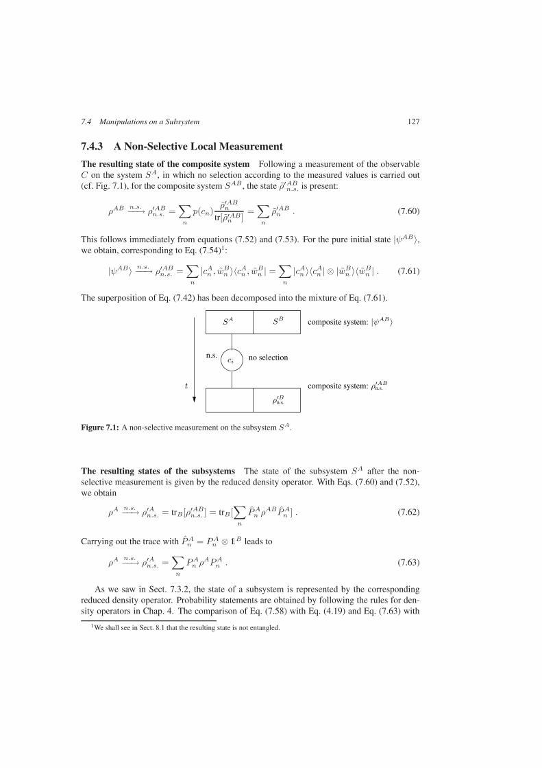
The resulting state of the composite system Following a measurement of the observableC on the system SA, in which no selection according to the measured values is carried out(cf. Fig. 7.1), for the composite system SAB , the state ρ′ABn.s. is present:

ρABn.s.−−→ ρ′ABn.s. =

∑

n

p(cn)ρ′ABn

tr[ρ′ABn ]=∑

n

ρ′ABn . (7.60)

This follows immediately from equations (7.52) and (7.53). For the pure initial state |ψAB〉,we obtain, corresponding to Eq. (7.54)1:

|ψAB〉 n.s.−−→ ρ′ABn.s. =∑

n

|cAn , wBn 〉〈cAn , wBn | =∑

n

|cAn 〉〈cAn | ⊗ |wBn 〉〈wBn | . (7.61)

The superposition of Eq. (7.42) has been decomposed into the mixture of Eq. (7.61).

SA

t

n.s.ci

SB

ρ′Bn.s.

no selection

composite system: |ψAB〉

composite system: ρ′ABn.s.

Figure 7.1: A non-selective measurement on the subsystem SA.

The resulting states of the subsystems The state of the subsystem SA after the non-selective measurement is given by the reduced density operator. With Eqs. (7.60) and (7.52),we obtain

ρAn.s.−−→ ρ′An.s. = trB[ρ′ABn.s. ] = trB [

∑

n

PAn ρABPAn ] . (7.62)

Carrying out the trace with PAn = PAn ⊗ 1B leads to

ρAn.s.−−→ ρ′An.s. =

∑

n

PAn ρAPAn . (7.63)

As we saw in Sect. 7.3.2, the state of a subsystem is represented by the correspondingreduced density operator. Probability statements are obtained by following the rules for den-sity operators in Chap. 4. The comparison of Eq. (7.58) with Eq. (4.19) and Eq. (7.63) with

1We shall see in Sect. 8.1 that the resulting state is not entangled.


(4.25) shows that: for the transitions between the reduced density operators as produced byselective or non-selective local measurements on a subsystem, the rules for density operatorsfrom Chap. 4 can be applied.

What can we say about the other subsystem SB? All the measurements on Bob’s subsys-tem SB in the case of non-selective measurements by Alice on SA can be described by thereduced density operator

ρ′Bn.s. = trA[ρ′ABn.s.] . (7.64)

We reformulate it with the aid of Eqs. (7.60) and (7.52) and find by using∑n P

An = 1AB the

result:

ρ′Bn.s = trA[∑

n

ρ′ABn ] = trA[∑

n

PAn ρAB] = trA[(

∑

n

PAn )ρAB] = trAρAB = ρB .

(7.65)

The density operator ρ′Bn.s of the subsystem SB after the non-selective measurement on SA isthe same as the density operator ρB before the measurement.

This is a remarkable result. Let us consider the situation in which the system SA is atAlice’s location and the system SB at Bob’s (spatially separated) location. In a preparationprocedure, bipartite systems are often produced in the state ρAB . It can be entangled. It isthen left open to Alice as to whether she carries our measurements of some observable C onher system or not. Bob cannot determine in any manner by measurements on his subsystemSB whether or not Alice has carried out measurements. The analogous statement for unitarymanipulations on the system SA has already been derived in Sect. 7.4.1.

7.5 Separate Manipulations on both Subsystems

7.5.1 Pairs of Selective Measurements

First, Alice carries out a measurement and obtains the result cn with the probability p(cn) =〈wBn |wBn 〉. The system is transformed after the selection described above into the compositestate |cAn , wBn 〉 (compare Fig. 7.2). If Bob makes a measurement following this selection, heobtains the value di with the conditional probability

p(di|cn) =|αni|2p(cn)

. (7.66)

This can be read off from Eqs. (7.44) and (7.55). The composite system is then transformedinto the product state |cAn , dBi 〉 after another selection for which Bob informs Alice of the resulthe has obtained. If, in reverse, first Bob and then – after selection according to the measuredvalue di – Alice makes a measurement, we obtain analogously (see Fig. 7.2) after the secondselection the same final state for the pair of measured values (cn, di). For the probabilities,we then have

p(cn|di) =|αni|2p(di)

. (7.67)

7.5 Separate Manipulations on both Subsystems 129

to outcome

selectionaccording

to outcome

selectionaccording

t

SBSA SBSA

cn di

di cn

|cAn 〉|cAn 〉 |dBi 〉

|cAn 〉 |wBn 〉 |vA

i 〉 |dBi 〉

|dBi 〉

composite system: |ψAB〉

Figure 7.2: A selective measurement on the subsystems SA and SB . Left: the measurement is firstcarried out on SA and then on SB ; right in the reverse order. A selection is carried out in each caseaccording to the measured values di and cn. The probability of obtaining the pair of measured values(cn, di) and the corresponding final state |cAn , dB

i 〉 is the same in both cases.

The joint probability p(cn, di) with which the pair of measured values (cn, di) is obtainedfrom selective local measurements is independent of the order in which they are carried out.One finds

p(cn, di) = p(cn|di)p(di) = p(di|cn)p(cn) = |αni|2 = 〈ψAB|PABni |ψAB〉 (7.68)

with the projection operator

PABni := |cAn , dBi 〉〈cAn , dBi | . (7.69)

The final state is PABni |ψAB〉 = |cAn , dBi 〉. Since the observables CA and DB of the localmeasurements commute, this could have been expected. We add that all of the statementsmade above for the pure initial state |ψAB〉 can be applied in the well-known manner whenthe initial state is a mixture with the density operator ρAB .

Instead of selecting after each local measurement, Alice and Bob can also find the state|cn, di〉 after a large number of measurements by referring to the result (cn, di). In this case,also, an exchange of information in both directions is necessary. It is a part of the preparationprocedure for the state |cAn , dBi 〉. In many cases, one is interested in the probabilities p(cn, di)with which the pairs of measured values (cn, di) occur. To find them, Alice and Bob meet aftercarrying out measurements on many systems and determine the relative frequency of the com-binations of measured values. These correlations of locally-obtained results are determinedby the preparation procedure of the initial state (7.42).


Mean values The dyadic decomposition of the operators CA ⊗DB has the form (compareEq. (7.51))

CA⊗DB =∑

n,i

cndi|cAn , dBi 〉〈cAn , dBi | . (7.70)

For its mean value in the state ρAB , we have∑

n,i

trAB[PABni ρ

AB]cndi = trAB

[(CA⊗DB) ρAB

]. (7.71)

The trace on the left side is the probability that in local measurements of CA and DB onthe subsystems SA and SB , the pair of measured values (cn, di) will be obtained. The meanvalue of the products of correlated local measured values is the same as the mean value ofthe product operator. We will make use of this fact, especially in Sects. 9.2.2 and 10.1, inconnection with non-local measurements.

7.5.2 Non-Local Effects: “Spooky Action at a Distance”?

For an improved understanding, it is helpful to confront the results of the preceding sectionswith a popular catchword. We consider the following situation: we carry out local measure-ments of the same observable C on a system in the state

|ψAB〉 =1√2(|cA1 , cB1 〉+ |cA2 , cB2 〉) (7.72)

(conventions as in Sect. 7.4.2). The possible results are c1 or c2. The probabilities of occur-rence of the pairs of measured values are

p(c1, c1) = p(c2, c2) =12

(7.73)

p(c1, c2) = p(c2, c1) = 0 . (7.74)

The measurements on SA yield, for example, the value c1. Then one often says, in an abbre-viated and sometimes misleading manner of speech, that the measurement has transformedthe composite system SAB into the state |cA1 , cB2 〉 and thereby the subsystem SB into the state|cB1 〉. This holds independently of the spatial separation between the system SA at Alice’s lo-cation and SB at Bob’s. In popular-scientific descriptions, this is often referred to as “spookyaction at a distance”2. Is the situation of quantum physics correctly characterised by this term?

We have seen the the preparation of quantum objects in a state |cA1 , cB1 〉 requires a selectionby Alice, a communication at most at the velocity of light between Alice and Bob, and aselection by Bob. This is most certainly not a case of instantaneous action at a distance.

2A. Einstein wrote concerning the quantum theory: “Ich kann aber deshalb nicht ernsthaft daran glauben, weil dieTheorie mit dem Grundsatz unvereinbar ist, dass die Physik eine Wirklichkeit in Zeit und Raum darstellen soll, ohnespukhafte Fernwirkung”. (A. Einstein in a letter to M. Born dated 3.3.1947 [EB 69]). Born’s translation: “I cannotseriously believe in it because the theory cannot be reconciled with the idea that physics should represent a reality intime and space, free from spooky actions at a distance”. We shall return to what Einstein understood to be “reality”in Chap. 10.

7.6 The Unitary Dynamics of Composite Systems 131

Perhaps the catchword is not meant to refer to states, and thereby to preparation proce-dures, but rather to measured values. If Alice obtains the value c1, then Bob, according toEq. (7.74), will with certainty find the value c1. This is also the case when the two measure-ments are carried out simultaneously. For a system prepared in the state (7.72), measurementsof the observable C on SA and SB yield completely correlated results. However, the occur-rence of the two results is not causally related. We are familiar with a similar situation in thecase of classical systems: as a preparation procedure, either a red or a blue ball is placed intoeach of two boxes. If the preparation procedure is known, then after opening one of the boxes,it can be predicted with certainty what the result of a simultaneous observation of the ball inthe other box will be. It is not necessary that the colour of the one ball be somehow connectedwith the colour of the other via some interaction which propagates with more than the velocityof light. Correlations are already determined by the preparation procedure.

By the comparison to the two-ball experiment, we wished to emphasize that in this situa-tion, the correlations are decisive. Not all statements about composite quantum systems canbe simulated by classical systems such as e.g. coloured balls. We will discuss this in detail inChap. 10. The section after the next contains a first demonstration of this.

How Alice prepares Bob’s subsystem in a state of her choice For every given ONB|s〉, |t〉, the state |ΦAB+ 〉 = 1√

2(|0A, 1B〉 − |1A, 2B〉) can always be written in the form

|ΦAB+ 〉 =1√2(|sA, tB〉 − |tA, sB〉) . (7.75)

Alice wants to transform the subsystem SB at Bob’s location into the state |sB〉. To do so,she makes a measurement on her system SA in the ONB |sA〉|tA〉 and informs Bob if hermeasurement yields the result associated with |tA〉. Then Bob can select accordingly amonghis subsystems. The result is a preparation procedure which leads Bob to quantum objects inthe state |sB〉. For this purpose, no quantum objects need be transmitted between Alice andBob. The entangled state serves as a tool (similar procedures are described in Sect. 11.2 andin connection with quantum teleportation in Sect. 11.3).

7.6 The Unitary Dynamics of Composite Systems

We consider unitary transformations of the composite system. The von Neumann equation(4.9) or (4.10) can be applied to composite systems according to the postulates

idρAB

dt= [HAB, ρAB(t)]− i

dρAB

dt= LABρAB(t) . (7.76)

with the Liouville operator LAB ∈ LA ⊗ LB . We employ the Schrödinger representation. Ifan interaction described by the Hamiltonian HAB

int = 0 is present between the subsystems SA

and SB , then the individual subsystems are open quantum systems. The overall Hamiltonianthen has the form

HAB = HA ⊗ 1B + 1A ⊗HB +HABint . (7.77)


The associated Liouville operator is found to be

LAB = LA + LB + LABint (7.78)

and it follows for the von Neumann equation:

idρAB

dt= (LA + LB + LABint )ρAB(t) . (7.79)

This leads to a differential equation for the reduced density operator ρA

idρA

dt= LAρA(t) + trB [LABint ρ

AB(t)] . (7.80)

To determine ρA(t), the complete equation (7.79) must be integrated. There are various ap-proximation methods to accomplish this. In Sect. 13.1 and Chap. 14, we will encounter anin-out approach to the dynamics of open systems, which is not based upon the differentialtime dependence of ρA(t) described by Eq. (7.80). Instead, it relates the final state ρA(tout) tothe initial state ρA(tin) by means of a superoperator.

7.7 A First Application of Entanglement: a ConjuringTrick

In the coming chapters, we will demonstrate repeatedly that entanglement is a central tool onwhich the effects of quantum information theory are based. Entanglement and the quantumcorrelations which arise from it can however also be a tool for the study of the fundamentals ofquantum theory. We wish to demonstrate this in answering the following underlying question:can effects of quantum theory be explained by means of classical physics – possibly in theframework of theories which have yet to be formulated? This will give us directly an exampleof an application for the formalism introduced in the preceding sections. In a wider context,we will come back to this question in Chap. 10.

7.7.1 The Conjuring Trick

A magician amazes his audience with the following trick: the audience sees the magician givesomething to his two assistants Alice and Bob. Alice and Bob then each go into separaterooms which are perfectly insulated against any exchange of information. In each room is anaudience. In each, a coin is tossed and, depending on the result of the toss, a question is askedof Alice or Bob. If the result is “heads”, then the question concerns the favourite colour; it canbe answered with either “red” or “green”. If the tossed coin gives “tails”, then the audience isto ask the question, “What is your favourite vegetable”, and the answer can be either “carrots”or “peas”. The question and answer are written down; one round is then finished. Alice, Boband the magician meet again, enter the question-and-answer pair in a list with the audience aswitnesses, and repeat the whole procedure again from the beginning. A large number of suchrounds is completed. At the end, the combined audience analyses the question-and-answerpairs, looking for correlations.

7.7 A First Application of Entanglement: a Conjuring Trick 133

There are four pairs of questions which can be divided into three cases: both are asked fora colour, one for a colour and the other for a vegetable, or both are asked for vegetables. Ineach performance, the following correlations are found:

Alice Bob

1st Case colour? colour?green! green!

To the pair of questions (colour?, colour?), the pair of answers (green!, green!)is given with a non-vanishing frequency.

2nd Case colour? vegetable?green! peas!

vegetable? colour?peas! green!

When one answers this combination of questions with “green!”, then the otheralways gives the appropriate answer “peas”.

3rd Case vegetable? vegetable?

To this combination of questions, one of the two assistants with certainty givesthe answer “carrots!”.

This is what the audience records.

7.7.2 Classical Correlations can give no Explanation

The audience sees that pairs of answers are given with a certain regularity. How did themagician arrange this? What was his trick? The audience presumes that Alice and Bob weregiven slips of paper on which a colour and a vegetable were written. They then read off theanswers to the questions correspondingly. The magician had prepared pairs of paper slips withdifferent abundances, so that precisely the correlations between the answers as listed abovewould be observed.

Assuming this were the case, then to produce the first case in the table, the magicianmust have given out slips which both had the colour “green” written on them. In order thatthe pairs of questions (colour?, vegetable?) and (vegetable?, colour?) would always beanswered correctly, the vegetable on both of these slips would have to be “peas” (secondcase). However, this would contradict the requirement that in the case of the third possiblecombination of questions (vegetable?, vegetable?) at least one of the assistants would answerwith “carrots”. The method with slips of paper thus does not yield the results observed. Wewant to demonstrate that the magician nevertheless need not possess paranormal abilities in


|r〉 ↔ red

|g〉 ↔ green

|P 〉 ↔ peas

|C〉 ↔ carrots

Figure 7.3: Bases in which the measurements are carried out for the conjuring trick. When pairs ofphotons are used, these are the analyser devices.

order to cause the observed correlations of the answers. It suffices for him to have someknowledge of entangled states.

7.7.3 The Trick

The magician’s trick consists of the fact that he does not use correlated classical systems suchas pairs of paper slips, but instead he makes use of entangled quantum systems. He gave toAlice and Bob each a subsystem of a bipartite systems, which was prepared to be in the state

|χAB〉 = N(|rA, rB〉 − a2|PA, PB〉) (7.81)

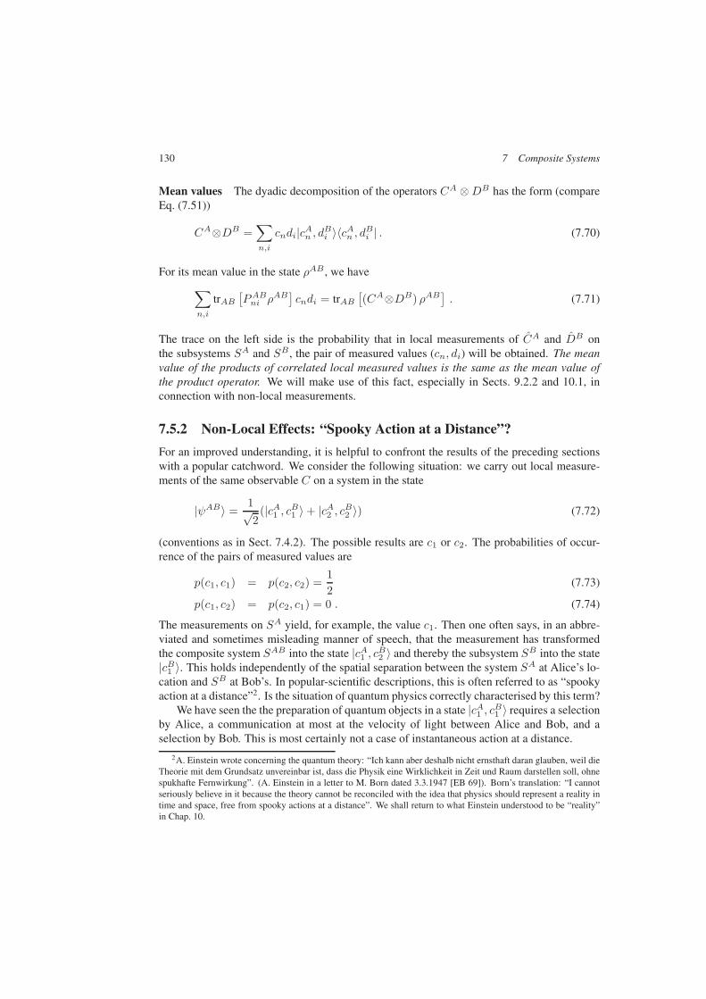
with a ∈ R and a = 0, a = 1. N is a normalisation factor and |r〉, |g〉 and |C〉, |P 〉 areorthonormal bases ofH2, which are rotated relative to one another (see Fig. 7.3).

|r〉 = a|P 〉+ b|C〉 (7.82)

|g〉 = b|P 〉 − a|C〉 (7.83)

with b ∈ R and a2 + b2 = 1. Resolution leads to

|P 〉 = a|r〉+ b|g〉 (7.84)

|C〉 = b|r〉 − a|g〉 . (7.85)

If Alice or Bob is asked for the colour, he or she carries our a measurement on the subsys-tem in the |P 〉, |C〉 basis and interprets the result with respect to the state to which the mea-surement leads, according to the rule |P 〉 ↔ “peas!” and |C〉 ↔ “carrots!”. Correspondingly,when the question is for the vegetable, the measurement is carried out in the rotated |r〉, |g〉basis and the answer is given according to the rule |r〉 ↔ “red!” and |g〉 ↔ “green!”. We canread off from the state |χAB〉 the probabilities with which particular pairs of answers will begiven.

To find the probabilities, we insert |P 〉 from Eq. (7.84) in various places into Eq. (7.81):

|χAB〉 = N(|rA, rB〉 − a2(a|rA〉+ b|gA〉)(a|rB〉+ b|gB〉)) (7.86)

|χAB〉 = N(|rA, rB〉 − a2(a|rA〉+ b|gA〉)|PB〉) (7.87)

|χAB〉 = N(|rA, rB〉 − a2|PA〉(a|rB〉+ b|gB〉)) . (7.88)

7.8 Quantum Gates for Multiple Qubit Systems 135

|r〉 from Eq. (7.82) inserted into |χAB〉 leads to:

|χAB〉 = N [(a|PA〉+ b|CA〉)(a|PB〉+ b|CB〉)− a2|PA, PB〉]= N(b2|CA, CB〉+ ab(|CA, PB〉+ |PA, CB〉)) . (7.89)

From Eqs. (7.86)–(7.89), we find the probabilities for the possible pairs of measurement re-sults and thus for the pairs of answers (compare Eq. (7.68)). From Eq. (7.86), for the pair ofquestions in the first case, the observed result is found:

p(gA, gB) = Na4b4 = 0 . (7.90)

Eqs. (7.87) and (7.88) lead to

p(gA, CB) = 0, p(CA, gB) = 0 . (7.91)

Therefore, when the pair of questions (colour?, vegetable?) is asked, and Alice answers with“green!”, then Bob always answers with “peas!” and vice versa. This reproduces the secondcase. Finally, we verify the third case with Eq. (7.89):

p(PA, PB) = 0 . (7.92)

Entanglement is the tool with which quantum magicians can carry out the tricks which classi-cal magicians cannot master.

Consequences The experimental implementations of the basic idea of the conjuring trickare not so simple as we described in Sect. 7.7.1. The results however agree well with thequantum theoretical predictions (compare Sect. 10.8).

The conjuring trick can be carried out in principle, but not with the means and methods ofclassical physics. Systems for which the results of measurements (Alice’s and Bob’s answers)are already predetermined before the measurement (Einstein’s reality) on the correspondingsubsystems (Einstein’s locality), such as is the case for the slips of paper, cannot be the causeof the observed correlations. This shows that local-realistic theories and the quantum theorycan lead to differing predictions. In our example: “the conjuring trick cannot be carried out”or “the conjuring trick can be carried out”; but only the predictions of quantum theory canbe experimentally verified. Thus, local-realistic alternative theories to the quantum theoryare refuted. We will describe additional experiments in Chap. 10 and then give more precisedefinitions for the concepts of Einstein reality and Einstein locality.

7.8 Quantum Gates for Multiple Qubit Systems

7.8.1 Entanglement via a CNOT Gate

The processing of quantum information is often explained schematically without referenceto an experimental implementation with the aid of quantum circuits. The essential deviceswhich are needed are: quantum wires; these are special quantum channels through whichquantum systems can propagate without being modified; and quantum gates, which effect


|x⊕ y〉

|x〉control qubit |x〉

target qubit |y〉

Figure 7.4: A CNOT gate.

unitary transformations of quantum systems. The systems are multi-qubits from the spacesH2 ⊗ H2 ⊗ H2 . . . ⊗ H2. Measurements permit reading out of the information. Owing tothe unitarity of their operations, quantum gates represent reversible processes. Measurementsare, in contrast, irreversible. Quantum computers are a network of quantum gates. We havealready encountered quantum gates for quantum systems inH2 in Sect. 3.4. We now move onto product spaces. In Chap. 12, we will assemble quantum circuits into quantum computers.

Entanglement via a CNOT gate A simple quantum gate which transforms a qubit productstate into an entangled state is the CNOT gate or controlled NOT gate, also called an XORgate. Its action on the computational basis ofHA2 ⊗HB2 is defined by

|x, y〉 → |x, y ⊕ x〉 (7.93)

with x, y, . . . ∈ 0, 1. This determines the action on an arbitrary vector fromHA2 ⊗HB2 . Thesymbol ⊕ denotes addition modulo 2, i. e. 1⊕ 1 = 0. In detail, this means that:

|0A, 0B〉 CNOT−→ |0A, 0B〉 (7.94)

|0A, 1B〉 CNOT−→ |0A, 1B〉 (7.95)

|1A, 0B〉 CNOT−→ |1A, 1B〉 (7.96)

|1A, 1B〉 CNOT−→ |1A, 0B〉 . (7.97)

From this, it follows that

(CNOT) · (CNOT) = 1 . (7.98)

Applying the matrix representation in the computational basis,

CNOT↔

1 0 0 00 1 0 00 0 0 10 0 1 0

, (7.99)

one can readily verify the unitarity property:

(CNOT)† = (CNOT)−1 . (7.100)

The qubits of the system A or B are called control qubits or target qubits (see Fig. 7.4).

7.8 Quantum Gates for Multiple Qubit Systems 137

H

H

=

H

H

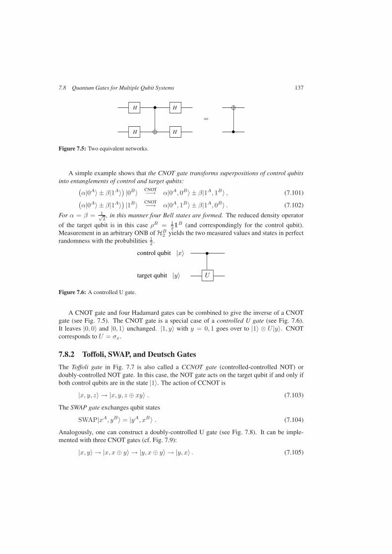
Figure 7.5: Two equivalent networks.

A simple example shows that the CNOT gate transforms superpositions of control qubitsinto entanglements of control and target qubits:

(α|0A〉 ± β|1A〉) |0B〉 CNOT−→ α|0A, 0B〉 ± β|1A, 1B〉 , (7.101)(α|0A〉 ± β|1A〉) |1B〉 CNOT−→ α|0A, 1B〉 ± β|1A, 0B〉 . (7.102)

For α = β = 1√2

, in this manner four Bell states are formed. The reduced density operator

of the target qubit is in this case ρB = 121

B (and correspondingly for the control qubit).Measurement in an arbitrary ONB ofHB2 yields the two measured values and states in perfectrandomness with the probabilities 1

2 .

U

control qubit |x〉

target qubit |y〉

Figure 7.6: A controlled U gate.

A CNOT gate and four Hadamard gates can be combined to give the inverse of a CNOTgate (see Fig. 7.5). The CNOT gate is a special case of a controlled U gate (see Fig. 7.6).It leaves |0, 0〉 and |0, 1〉 unchanged. |1, y〉 with y = 0, 1 goes over to |1〉 ⊗ U |y〉. CNOTcorresponds to U = σx.

7.8.2 Toffoli, SWAP, and Deutsch Gates

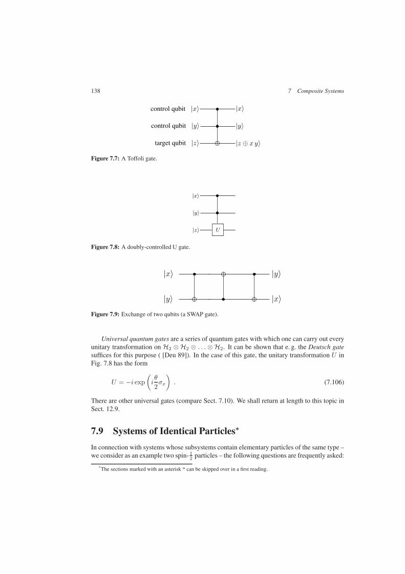
The Toffoli gate in Fig. 7.7 is also called a CCNOT gate (controlled-controlled NOT) ordoubly-controlled NOT gate. In this case, the NOT gate acts on the target qubit if and only ifboth control qubits are in the state |1〉. The action of CCNOT is

|x, y, z〉 → |x, y, z ⊕ xy〉 . (7.103)

The SWAP gate exchanges qubit states

SWAP|xA, yB〉 = |yA, xB〉 . (7.104)

Analogously, one can construct a doubly-controlled U gate (see Fig. 7.8). It can be imple-mented with three CNOT gates (cf. Fig. 7.9):

|x, y〉 → |x, x⊕ y〉 → |y, x⊕ y〉 → |y, x〉 . (7.105)


|x〉

|y〉

|z ⊕ x y〉

control qubit |x〉

control qubit |y〉

target qubit |z〉

Figure 7.7: A Toffoli gate.

U|z〉

|x〉

|y〉

Figure 7.8: A doubly-controlled U gate.

|x〉

|y〉

|y〉

|x〉Figure 7.9: Exchange of two qubits (a SWAP gate).

Universal quantum gates are a series of quantum gates with which one can carry out everyunitary transformation on H2 ⊗ H2 ⊗ . . . ⊗ H2. It can be shown that e. g. the Deutsch gatesuffices for this purpose ( [Deu 89]). In the case of this gate, the unitary transformation U inFig. 7.8 has the form

U = −i exp(iθ

2σx

). (7.106)

There are other universal gates (compare Sect. 7.10). We shall return at length to this topic inSect. 12.9.

7.9 Systems of Identical Particles∗

In connection with systems whose subsystems contain elementary particles of the same type –we consider as an example two spin-1

2 particles – the following questions are frequently asked:

*The sections marked with an asterisk * can be skipped over in a first reading.

7.9 Systems of Identical Particles∗ 139

The particles are Fermions and their composite states must be antisymmetric with respect toexchange of the states of the individual particles. Therefore, they must take a form similarto the Bell vectors |Φ−〉 or |Ψ−〉. Why can we not construct e.g. a teleportation procedurebased on this always-present “natural” entanglement? And conversely, how can we implementteleportation with Fermions in a symmetrically-entangled state |Φ+〉?

Identical particles Identical particles have the same values of all their intrinsic propertiessuch as mass, charge, spin etc. Electrons for example can be distinguished from positronsbut not from each other. They cannot be marked and therefore have no individuality. Anidentification is not possible.

To describe systems of identical particles, one can begin with enumerated distinguish-able particles and then remove their distinguishability. We restrict our considerations to2-particle systems. The generalisation to more particles is straightforward. The state vec-tors of two distinguishable particles with the numbers (1) and (2) lie in the product spaceH(1)(2) = H(1)⊗H(2). According to the postulates, the states of identical particles are eithercompletely symmetric in their particle numbers (Bosons, with integral spins), or completelyantisymmetric (Fermions, with half-integral spins). Their state vectors lie correspondingly insubspaces of H(1)(2), which we denote by H(1)(2)

+ and H(1)(2)− . These subspaces are them-

selves not product spaces. If |u(1)〉 and |v(2)〉 are ONB of H(1) or H(2), respectively,

then the bases of e.g. H(1)(2)− are given by |n, i〉− := 1√

2(|n(1), i(2)〉 − |i(1), n(2)〉) with

1 ≤ n ≤ dimH(1) and 1 ≤ i ≤ dimH(2). Without any interactions at all, the symmetry pos-tulate leads to states which are formally entangled in terms of their non-observable particlenumbers.

Even with the aid of observables, no identification of the particles is allowed. Observablesmust therefore be invariant under permutations of the particle numbers. The postulates forprojection measurements apply. They are formulated with respect to the spaces H(1)(2)

+ or

H(1)(2)− . A consequence of this is that measurements or unitary dynamical evolutions cannot

produce transitions between Bosons and Fermions.

Particles in two different regions of space We clarify the essential points using the exam-ple of two spin-1

2 particles with external degrees of freedom. H(1) and H(2) are thus alreadyassumed to be product spaces for the external degrees of freedom (vectors |α〉 and |β〉) andfor the spins (vectors |0〉 and |1〉). A possible state is then e.g.

|Λ(1)(2)〉 =1√2

(|α, 0〉(1) ⊗ |β, 1〉(2) − |β, 1〉(1) ⊗ |α, 0〉(2)

). (7.107)

In order to make the connection to the preceding sections, we discuss a situation in which〈α|β〉 = 0 holds. The states |α〉 and |β〉 are orthogonal. This is the case e.g. when theparticles have differing directions of their momenta or when the wavefunctions 〈r|α〉 and 〈r|β〉are nonzero only in a restricted spatial region Gα or Gβ , where Gα and Gβ do not overlap(Gα ∩Gβ = ∅). Then, one can register a Fermion only in Gα or in Gβ , but not outside them.However, statements about the particle numbers (1) or (2) are not possible. Gα or Gβ can bee.g. different locations at which Alice A or Bob B have set up their measurement apparatus


which can carry out measurements in spin space. If Alice’s apparatus registers a signal, this atthe same time represents a measurement in configuration space, i.e. Gα is registered. For thedescription of this situation, we can introduce an abbreviated form which reflects the fact thatin the case Gα ∩ Gβ = ∅, the state |α〉 (i.e. the location Gα, Alice) is always correlated with|0〉 and the state |β〉 (i.e. the location Gβ , Bob) is always correlated with |1〉:

|Λ(1)(2)〉 ↔ |ΛAB〉 = |0A, 1B〉 . (7.108)

With respect to all the measurements which can be carried out by Alice and Bob, the productstate |ΛAB〉 is equivalent to the state |Λ(1)(2)〉. If Alice measures the observable σz , she alwaysfinds the spin state |0〉. This is the content of Eq. (7.107).

If Alice measures the observable σx, the result of the measurement can yield e.g. theeigenvalue |1x〉 and the 2-Fermion system is transformed after selection into the state

|ΛAB〉 → |Λ′AB〉 = |1Ax , 1B〉 . (7.109)

|Λ′AB〉 can again be written in the complete form |Λ′(1)(2)〉. To this end, we replace |0〉 on theright-hand side of Eq. (7.107) by |1x〉. The probability of this result is |〈Λ(1)(2)|Λ′(1)(2)〉|2 =|〈ΛAB |Λ′AB〉|2. As a result of the orthonormalisation 〈α|β〉 = 0, the vector |ΛAB〉 inEq. (7.108) is a product vector in HAB .

Utilisable and non-utilisable entanglement The state introduced above, |n, i〉−, is a su-perposition, from which measurable interference effects can result in particular physical sit-uations. The fact that the particles cannot be distinguished has physical consequences. Theenergy spectrum of the helium atom is an example of this. In the following sections, how-ever, we shall discuss other physical questions. The entanglement for example in the state1√2(|0(1), 1(2)〉− |1(1), 0(2)〉) is related to the indistinguishable particle numbers. They do not

denote subsystems. Since this formal entanglement cannot be used, it cannot serve as a toolfor quantum-mechanical information processing. It is not utilisable for this purpose.

Only the entanglement with the states |α〉 and |β〉 with 〈α|β〉 = 0, as in the state |Λ(1)(2)〉of Eq. (7.107), opens up the possibility of intercession via |α〉 and |β〉. As we have alreadyseen, then |Λ(1)(2)〉 becomes equivalent to a non-entangled product state |ΛAB〉. If we nowform e.g. by superposition with an additional state

|Ω(1)(2)〉 =1√2

(|α, 1〉(1) ⊗ |β, 0〉2 − |β, 0〉(1) ⊗ |α, 1〉(2)

)↔ |ΩAB〉 = |1A, 0B〉

(7.110)

the state vector

|Ψ(1)(2)+ 〉 :=

1√2

(|Λ(1)(2)〉+ |Ω(1)(2)〉

), (7.111)

then we can read off from the abbreviated notation

|Ψ(1)(2)+ 〉 ↔ |ΨAB

+ 〉 =1√2

(|0A, 1B〉+ |1A, 0B〉) (7.112)

7.10 Complementary Topics and Further Reading 141

that the Bell state |ΨAB+ 〉 has been formed. In spite of the addition in Eq. (7.112), it has the

symmetry properties required for the description of two identical Fermions. At the same time,a utilisable entanglement has come about by the superposition described by Eq. (7.111).

If the condition 〈α|β〉 = 0 is not fulfilled in a physical situation, it can be expected thatadditional effects will occur in the course of the information processing, which are due to theindistinguishability of the particles. One can also switch on and off the coupling 〈α|β〉 = 0 inthe form of a time-dependent exchange coupling and thereby produce an entanglement only atcertain times. We mention also that the symmetry or antisymmetry property is automaticallytaken into account within the framework of the second quantisation.

7.10 Complementary Topics and Further Reading

• For “proper mixtures” and “improper mixtures”: [d’Es 95], [d’Es 99].

• Local measurements and the requirements of the theory of relativity: [PT 04].

• The idea that the whole is more than the sum of its parts is referred to in philosophy asholism. There is a whole series of philosophical analyses in which the attempt is madeto give this idea a precise meaning in many different fields from sociology to physics,and to investigate its consequences. For the natural-philosophical question as to whetherthere is a holism in physics, quite new aspects have resulted from the study of entangledstates in composite systems (see [Pri 81, Sects. 3.7, 5.6, 6.3]). Two differing analyses ofthis question are introduced in [Esf 04] and [See 04] (cf. [Esf 06]). There, more detailedliterature is also cited. See also [Hea 99].

• For the conjuring trick: [Har 93], [Har 98].

• Experiments on the conjuring trick: [Har 92], [TBM 95], [DMB 97], [BBD 97].

• An overview of quantum gates for qubits: [DiV 98], [Bra 02].

• In utilising coupled quantum dots or neutral atoms in microtraps as tools for quantuminformation processing, effects occur which are based upon the indistinguishability ofparticles. For details and further literature, see: [ESB 02].


7.11 Problems for Chapter 7

Prob. 7.1 [for 7.3.2]: Show that ρA and ρB in Eq. (7.34) have the properties required of adensity operator.

Prob. 7.2 [for 7.4 and 7.5]: Confirm the results of Sects. 7.4 and 7.5 for the case that theinitial state was not a pure state |ψAB〉, but rather a mixture, ρAB .

Prob. 7.3 [for 7.5.2]: Prove Eq. (7.75).

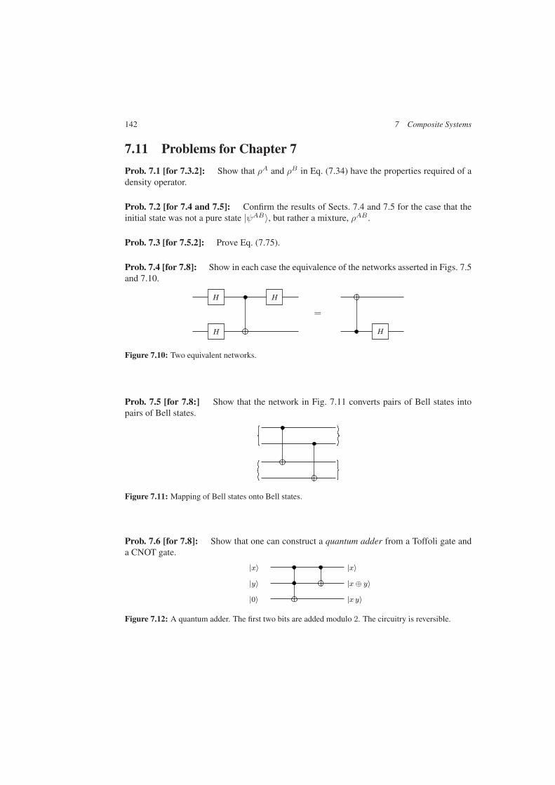
Prob. 7.4 [for 7.8]: Show in each case the equivalence of the networks asserted in Figs. 7.5and 7.10.

=

H

HH

H

Figure 7.10: Two equivalent networks.

Prob. 7.5 [for 7.8:] Show that the network in Fig. 7.11 converts pairs of Bell states intopairs of Bell states.

Figure 7.11: Mapping of Bell states onto Bell states.

Prob. 7.6 [for 7.8]: Show that one can construct a quantum adder from a Toffoli gate anda CNOT gate.

|x〉|y〉|0〉

|x〉|x⊕ y〉|x y〉

Figure 7.12: A quantum adder. The first two bits are added modulo 2. The circuitry is reversible.

Documents

7 Composite Systems