7 Field Plot Technique & Experimental Design. Field Plot technique pertains to the study of kind of field plots best suited for a particular type of experiment

7Field Plot Technique & Experimental Design

Field Plot technique pertains to the study of kind of field plots best suited for a particular type of experiment. It is important that the most efficient type and arrangement of plots be used in each particular experiment in order to assure reliable results.

Factors that Affect the conduct of Field Experiment• Soil fertility status (Moisture, nutrient etc)• Environment• Genotype

Variable soil fertility Heterogeneity can be reduced• Replication/ Blocking• Plot size (0.1 to 0.01 acre)• Interplot competetion or border effect

Blocking• Blocks are made

– To make expt units more uniform

– Thus making within block variation more

• Number of blocks is equal to number of reps

Slope

10%

Slope

6%

Slope

2%

High Medium LowFertility

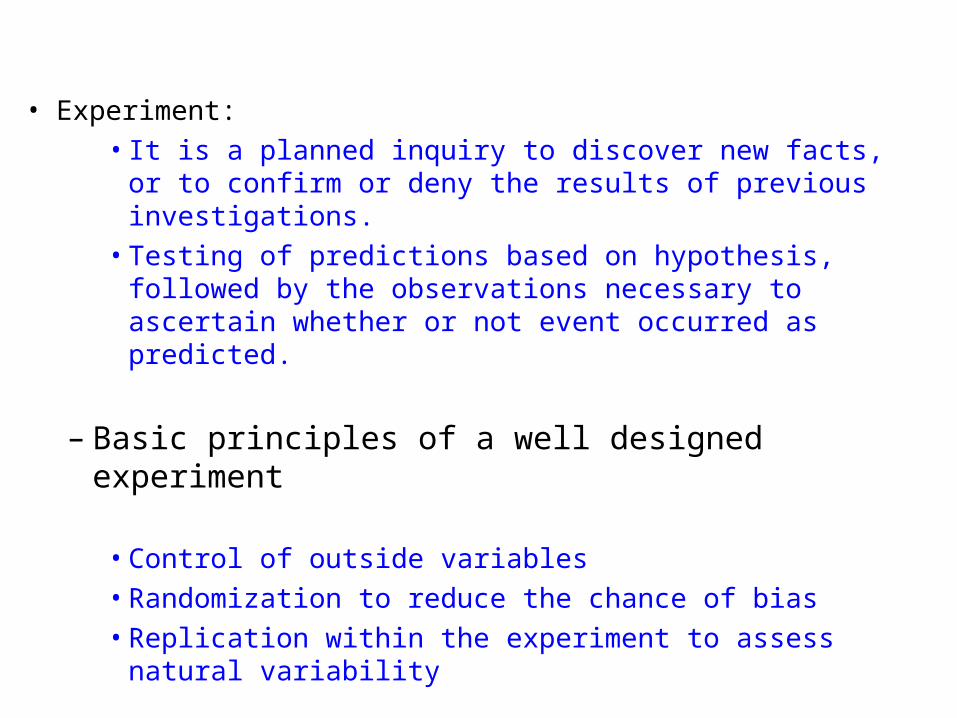
• Experiment:• It is a planned inquiry to discover new facts, or to

confirm or deny the results of previous investigations.• Testing of predictions based on hypothesis, followed

by the observations necessary to ascertain whether or not event occurred as predicted.

– Basic principles of a well designed experiment

• Control of outside variables• Randomization to reduce the chance of bias• Replication within the experiment to assess natural

variability

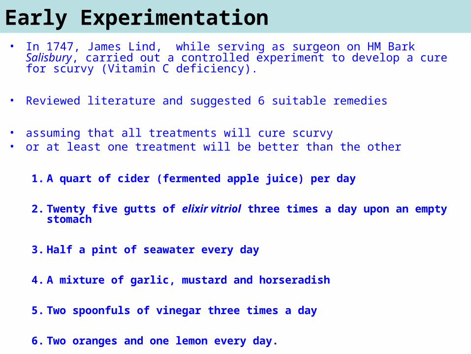
Early Experimentation• In 1747, James Lind, while serving as surgeon on HM Bark Salisbury, carried out a

controlled experiment to develop a cure for scurvy (Vitamin C deficiency).

• Reviewed literature and suggested 6 suitable remedies

• assuming that all treatments will cure scurvy • or at least one treatment will be better than the other

1. A quart of cider (fermented apple juice) per day

2. Twenty five gutts of elixir vitriol three times a day upon an empty stomach

3. Half a pint of seawater every day

4. A mixture of garlic, mustard and horseradish

5. Two spoonfuls of vinegar three times a day

6. Two oranges and one lemon every day.

• Selected 12 men from the ship, all suffering from scurvy,

• The men were paired, which provided replication.

• randomized allocation of subjects to treatments was missing

• Two weeks later

• The men who had been given citrus fruits recovered dramatically within a week.

• One of them returned to duty after 6 days and the other became nurse to the rest.

• The others experienced some improvement, but nothing was comparable to the citrus fruits, which were proved to be substantially superior to the other treatments.

Steps in Experiments

• Hypothesis• Treatments• Measures to reduce variation• Replication• Observations• Results • Significance of differences• Conclusion

• Statistical Hypothesis:– There are generally two forms of a statistical

hypothesis• null (typically represented as H0) : no differences exit

among treatments or treatments are similar – Rejection of null hypothesis will prove that there are

differences among treatments hence justifying research hypothesis

• alternative (typically symbolised as H1 - this is the research hypothesis - the one we are really interested in showing support for!)

– At least one of the treatment is significantly different

Some basic definitions

• Experimental unit: – it is piece of experimental material to which a treatment is assigned

• Replication:– Appearance of one treatment more than once in experiment is

called replication

• Randomization:– Each treatment has equal chance of being assigned to any

experimental unit

• Experimental error:– Variation among the experimental units which are treated alike

• Degree of freedom:– the number of values in the final calculation of a statistic that are

free to vary

– The number of independent pieces of information that go into the estimate of a parameter is called the degrees of freedom (df)

Randomization

• Randomization by lot– For 4 treatments and 3 reps= 12 expt

units– Make 12 pieces of paper, write down

1-12 on these pieces, fold the pieces, place them in box and shake thoroughly

– Pick pieces one by one and allot treatment 1 to first 3 numbers drawn

• Random number table – Select a starting point in random

number table– Select first twelve three digit number in

any direction from starting point– Rank them smallest to largest (ranks

correspond to expt unit)– Assign treatment 1 to first 3 numbers

(expt unit)

Sequence Random Number

Rank (expt unit #)

Treatment

1 481 5 A

2 516 6 A

3 991 12 A

4 062 1 B

5 804 11 B

6 675 9 B

7 154 2 C

8 437 4 C

9 571 7 C

10 769 10 D

11 639 8 D

12 428 3 D

• Analysis Of Variance. – This procedure employs the statistic (F) to test the

statistical significance of the differences among the obtained MEANS

• two estimates of a population variance are calculated – Variations among treatment means– Variation among experimental units within treatments

(experimental error)

• Calculation of statistic F

Types of Experiments

• Laboratory• Controlled environment• Green house• Field

– Yield testing

– Fertilizer response

– Pesticide efficacy

– Herbicide efficacy

– Water requirement

Basic Experimental designs

• Experimental design:– It is a rule or formal plan for the assignment of treatments to be used to the

experimental units (plots).

– Experimental design differ• Grouping of plots prior treatment application• Restrictions on randomization of treatments

• Why Experiments are designed– To facilitate the application of treatment, operations and recording of data

– To provide information required to perform tests of significance and to convert interval estimates

– To increase precision by planned grouping of plots and elimination of group differences from experimental error

– To provide an estimate of experimental error

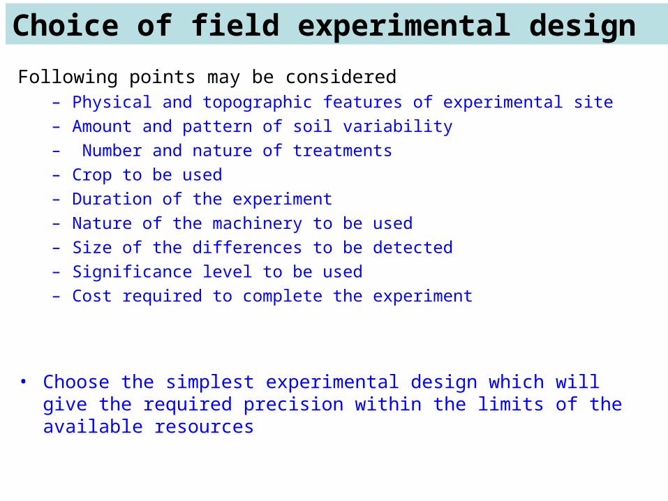
Choice of field experimental design

Following points may be considered– Physical and topographic features of experimental site

– Amount and pattern of soil variability

– Number and nature of treatments

– Crop to be used

– Duration of the experiment

– Nature of the machinery to be used

– Size of the differences to be detected

– Significance level to be used

– Cost required to complete the experiment

• Choose the simplest experimental design which will give the required precision within the limits of the available resources

Experimental Designs

• Completely randomized design

• Randomized complete block design

• Latin square design

• Factorial Design

• Split Plot Design

• Augmented Design

CRD Advantages, disadvantages and usesAdvantages:• Flexibility:

– Any number of treatments and any number of replications– Replication per treatment need not to be the same

• Simple statistical analysis– The analysis is not complicated despite unequal replication of treatment

• Missing plots– The analysis is not complicated by missing data

• Maximum error degree of freedom– No other expt. Design provide higher df (e) with similar no. plots and

treatments

Disadvantage• Low precision if Expt. Units are not uniform

– i.e. why it is used mainly in lab, green house and controlled environment expts.

It can be used/ Application– Experimental unit is more uniform– Number of expt. Units may damaged– Number of units is limited (it provides maximum error df)

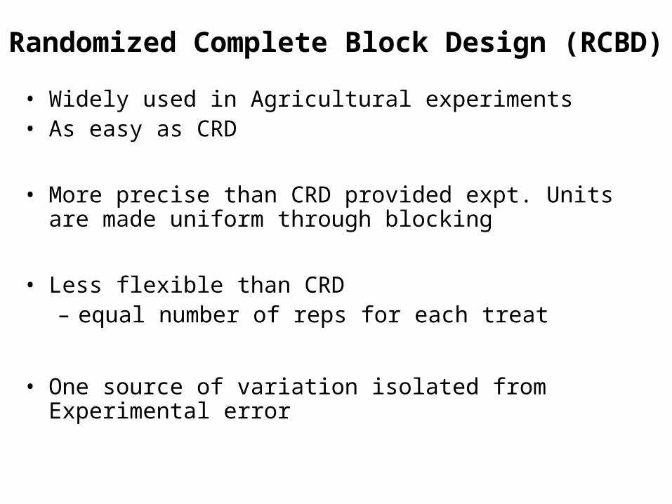
Randomized Complete Block Design (RCBD)

• Widely used in Agricultural experiments• As easy as CRD

• More precise than CRD provided expt. Units are made uniform through blocking

• Less flexible than CRD – equal number of reps for each treat

• One source of variation isolated from Experimental error

RCBD

ADVANTAGES– Remove one source of variation– Any no. of treatments and any no. of blocks (but each treatment must

be replicated in each block)– Statistical analysis is simple– Broaden the scope of trial by blocking for different conditions

DISADVANTAGES– Missing data cause difficulty in analysis– Assignment of treatment in wrong block– Less efficient if more than one source of unwanted variation– Less efficient in than CRD if expt units are uniform

USES – It can be used to eliminate source of unwanted variation– Provides unbiased estimates of the means of blocking

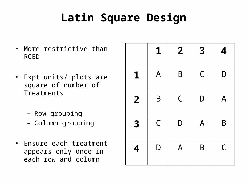
Latin Square Design

• More restrictive than RCBD

• Expt units/ plots are square of number of Treatments

– Row grouping– Column grouping

• Ensure each treatment appears only once in each row and column

1 2 3 4

1 A B C D

2 B C D A

3 C D A B

4 D A B C

Randomization

• 4 Treatments A, B, C, D• First row in alphabetical order• In subsequent row - shift letter

one position –

• Randomize Order of the rows (e.g. 2, 1, 3, 4)

• Randomize Order of the column (e.g. 4, 2 ,3, 1)

1 2 3 4

1 A B C D

2 B C D A

3 C D A B

4 D A B C

4 2 3 1

2 A C D B

1 D B C A

3 B D A C

4 C A B D

1 2 3 4

2 B C D A

1 A B C D

3 C D A B

4 D A B C

Comparison of Means• ANOVA• Range Tests

– Duncan’s Multiple Range Test (DMR)

– Least Significant Differences (LSD)

– Tukey’s Test

• LSD provides a valid test criteria in 2 situations

– Making comparisons planned in advance of data observed- (treatment with control)

– Comparing adjacent ranked means (to choose a winner)

• LSD should not be used – For all possible pair-wise comparisons

– Making more comparisons > no. df Treatment

Factorial Design• The experiment whose design consists of two or more factors,

whose experimental units take on all possible combinations of these levels across all such factors.

• An experiment in which an extra factor (second) is introduced into a study by dividing the large experimental units (whole unit) for the first factor into smaller experimental units (sub-units) on which the different levels of the second factor will be applied.

• Each whole unit is a complete replicate of all the levels of the second factor (RBD). The whole unit design may be CRD, RCBD or LS design.

ADVANTAGES• If an experiment is designed to study one factor, a second factor

may be included at very little cost.

• Since sub-unit variance is generally less than whole unit variance, the sub-unit treatment factor and the interaction are generally tested with greater sensitivity.

Split Plot Design

DISADVANTAGES• Analysis is complicated by the presence of two experimental error

variances, which leads to several different SE for comparisons.

• High variance and few replications of whole plot units frequently leads to poor sensitivity on the whole unit factor.

POSSIBLE APPLICATIONS• Experiments in which one factor requires larger experimental units

than the other factor.

• Experiments where greater sensitivity may be desired for one factor than for the second factor.

• Introduction of a new factor into an experiment which is already in progress.

Split Plot Design

Augmented Design• In agricultural experiments often the existing practices or check

varieties called control treatments are compared with new varieties or germplasms collected through exotic or domestic collections, called test treatments.

• In some cases experimental material for test treatments is limited and it is not possible to replicate them in the design.

• However, adequate material is available for replicating control treatments in the design. Augmented Designs are useful for these experimental situations.

• In an augmented randomized complete block design, the test treatments are replicated once in the design and control treatments appear exactly once in each block.

– It provides an estimate of experimental error for comparing test entries with check or control Varieties

– It provides a way of adjusting the yield of new selections for differences from block to block

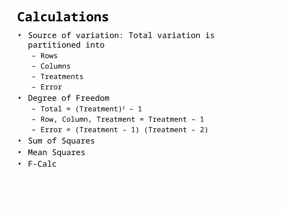
Calculations• Source of variation: Total variation is partitioned into

– Rows

– Columns

– Treatments

– Error

• Degree of Freedom– Total = (Treatment)2 – 1

– Row, Column, Treatment = Treatment – 1

– Error = (Treatment – 1) (Treatment – 2)

• Sum of Squares• Mean Squares• F-Calc

1 2 3 4 5

1 A 33.8 B 33.7 D 30.4 C 32.7 E 24.4

2 D 37 E 28.8 B 33.5 A 34.6 C 33.4

3 C 35.8 D 35.6 A 36.9 E 26.7 B 35.1

4 E 33.2 A 37.1 C 37.4 B 38.1 D 34.1

5 B 34.8 C 39.1 D 32.7 E 37.4 A 36.4

A B C D E

Treat Sum 178.8 175.2 178.4 174.5 145.8

Treat Mean 35.76 35.04 35.68 34.9 29.16

1 2 3 4 5 SUM Mean

1 33.8 33.7 30.4 32.7 24.4 155 31.0

2 37 28.8 33.5 34.6 33.4 167.3 33.5

3 35.8 35.6 36.9 26.7 35.1 170.1 34.0

4 33.2 37.1 37.4 38.1 34.1 179.9 36.0

5 34.8 39.1 32.7 37.4 36.4 180.4 36.1

SUM 174.6 174.3 170.9 169.5 163.4 852.7 170.5

Mean 34.92 34.86 34.18 33.9 32.68 170.54 34.1

Correction Factor = (GT)2/Total Observ. 29083.89

Total Sum of squares = (33.8)2 + -----+(36.4)2 - Cf 296.66

Row SS = 1/5 *(155)2+ -----+(180.4)2 -cf 87.40

Column SS= 1/5 *(174.6)2+ -----+(163.4)2 -cf 16.56

Treat SS = 1/5 *(178.8)2+ -----+(145.8)2 -cf 155.89

Error SS = Total SS - Row SS- Col SS - TreatSS 36.80

Degree of freedom– the number of values in the final calculation of a statistic that are free

to vary

– The number of independent pieces of information that go into the estimate of a parameter is called the degrees of freedom (df)

– In general, the degrees of freedom of an estimate is equal to the number of independent scores that go into the estimate minus the number of parameters estimated as intermediate steps in the estimation of the parameter itself.

– Imagine you are picking people to play in a team. You have eleven positions to fill and eleven people to put into those positions. How many decisions do you have? In fact you have ten, because when you come to the eleventh person, there is only one person and one position, so you have no choice. You thus have ten 'degrees of freedom' as it is called.

– Likewise, when you have a sample, the degrees of freedom to allocate people in the sample to tests is one less than the sample size. So if there are N people in a sample, the degrees of freedom is N-1.

Completely Randomized Design(CRD)

One-way ANOVA

• Experimental Unit:– Piece of experimental material which is assigned with treatment

– It may be • human• Animal• Test tubes• Pots• Field plots

• Treatment:– It is a procedure whose effect is to be noted on expt. Unit

• Medicine• Nutrients • Herbicides• Pesticides

RCBD – One Missing Value

Blocks

Treatment Rep 1 rep 2 Rep 3 Rep 4 Total

1 32.1 35.6 41.9 35.4 145

2 30.1 31.5 37.1 30.8 129.5

3 25.4 27.1 33.8 31.1 117.4

4 24.1 33 31.4 88.5

5 26.1 31 33.8 31.9 122.8

6 23.2 24.8 26.7 26.7 101.4

Total 161 183 173.3 187.3 704.9

Missing Data

• One Missing value

X = tT + rR – G

(t-1)(r-1)

X = Missing value

t = Number of treatment

r = Number of Repeats

T = Total of treatment with a missing value

R = Total of replication with a missing value

G = grand total with a missing value

X = (6*88.5) + (4*173.3) – 704.9

(6-1) (4-1)

X = 531 + 693.2 – 704.9

5*3

X = 34.62

REPS

Treatment 1 2 3 4 5 Total

1 22.3 21.8 21.2 20 85.3

2 18.3 18.5 21.5 17.3 75.6

3 17.2 17.2 17.9 16.7 69

4 14.9 12.6 13.1 14.4 12.4 67.4

Total 72.7 51.6 49.5 57.1 66.4 297.3

RCBD – More than One Missing Value

Missing DataMore than one Missing value

1. Approximation1. 85.3/4 = 21.25

2. 69.0/4 = 17.2

Treatment REPS

1 2 3 4 5 Total

1 22.3 21.8 21.25 21.2 20 106.55

2 18.3 18.5 21.5 17.3 75.6

3 17.2 17.2 17.9 17.2 16.7 86.2

4 14.9 12.6 13.1 14.4 12.4 67.4

Total 72.7 51.6 70.75 74.3 66.4 335.75


Calculation for first ValueX = tT + rR – G

(t-1)(r-1)

X = Missing value






X = (4*75.6) + (5*51.6) – 335.8

(4-1) (5 -1)

X = 302.4 + 258.0 – 335.8

3 * 4

X = 18.7

Treatment REPS

1 2 3 4 5 Total

1 22.3 21.8 21.2 20 85.3

2 18.3 18.7 18.5 21.5 17.3 94.3

3 17.2 17.2 17.9 17.2 16.7 86.2

4 14.9 12.6 13.1 14.4 12.4 67.4

Total 72.7 70.3 49.5 74.3 66.4 333.2


Calculation for Second ValueX = tT + rR – G

(t-1)(r-1)

X = Missing value






X = (4*85.3) + (5*49.5) – 333.2

(4-1) (5 -1)

X = 341.2 + 247.5 – 333.2

3 * 4

X = 21.3

Treatment REPS

1 2 3 4 5 Total

1 22.3 21.8 21.3 21.2 20 106.6

2 18.3 18.7 18.5 21.5 17.3 94.3

3 17.2 17.2 17.9 16.7 87.8

4 14.9 12.6 13.1 14.4 12.4 67.4

Total 72.7 70.3 70.8 75.9 66.4 356.1


Calculation for Third ValueX = tT + rR – G

(t-1)(r-1)

X = Missing value






X = (4*69) + (5*57.1) – 337.3

(4-1) (5 -1)

X = 276 + 285.5 – 333.2

3 * 4

X = 18.8

Treatment REPS

1 2 3 4 5 Total

1 22.3 21.8 21.3 21.2 20 106.6

2 18.3 18.7 18.5 21.5 17.3 94.3

3 17.2 17.2 17.9 18.8 16.7 87.8

4 14.9 12.6 13.1 14.4 12.4 67.4

Total 72.7 70.3 70.8 75.9 66.4 356.1

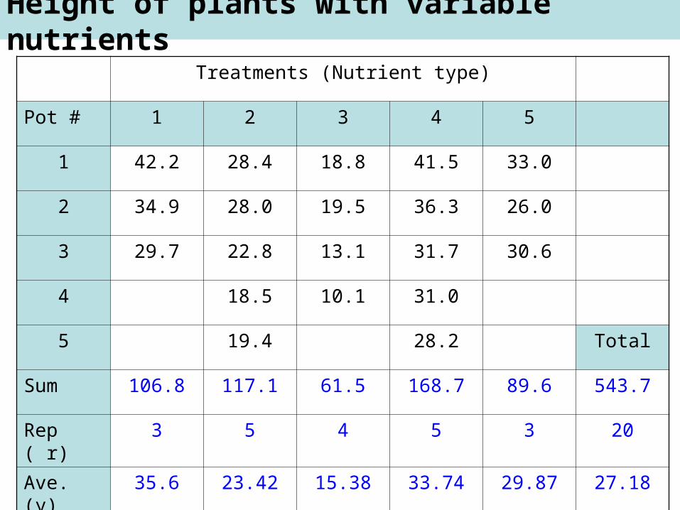
Height of plants with variable nutrients

Treatments (Nutrient type)

Pot # 1 2 3 4 5

1 42.2 28.4 18.8 41.5 33.0

2 34.9 28.0 19.5 36.3 26.0

3 29.7 22.8 13.1 31.7 30.6

4 18.5 10.1 31.0

5 19.4 28.2 Total

Sum 106.8 117.1 61.5 168.7 89.6 543.7

Rep ( r) 3 5 4 5 3 20

Ave. (y) 35.6 23.42 15.38 33.74 29.87 27.18

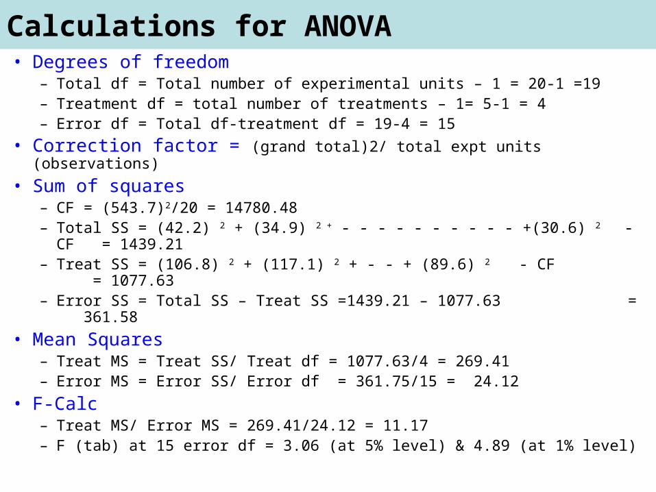
Calculations for ANOVA• Degrees of freedom

– Total df = Total number of experimental units – 1 = 20-1 =19– Treatment df = total number of treatments – 1= 5-1 = 4– Error df = Total df-treatment df = 19-4 = 15

• Correction factor = (grand total)2/ total expt units (observations)

• Sum of squares– CF = (543.7)2/20 = 14780.48– Total SS = (42.2) 2 + (34.9) 2 + - - - - - - - - - - +(30.6) 2 - CF = 1439.21– Treat SS = (106.8) 2 + (117.1) 2 + - - + (89.6) 2 - CF = 1077.63– Error SS = Total SS – Treat SS =1439.21 – 1077.63 = 361.58

• Mean Squares– Treat MS = Treat SS/ Treat df = 1077.63/4 = 269.41– Error MS = Error SS/ Error df = 361.75/15 = 24.12

• F-Calc– Treat MS/ Error MS = 269.41/24.12 = 11.17– F (tab) at 15 error df = 3.06 (at 5% level) & 4.89 (at 1% level)

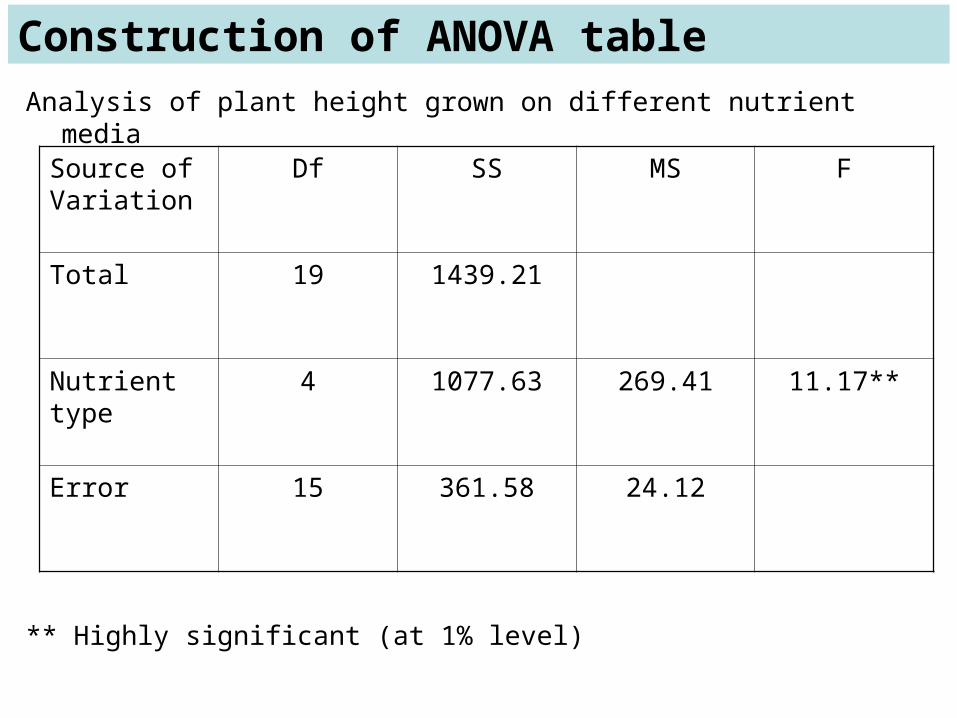
Construction of ANOVA table

Analysis of plant height grown on different nutrient media

** Highly significant (at 1% level)

Source of Variation

Df SS MS F

Total 19 1439.21

Nutrient type 4 1077.63 269.41 11.17**

Error 15 361.58 24.12

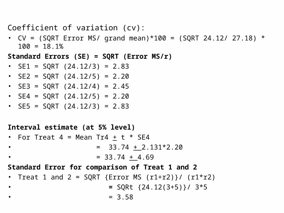
Coefficient of variation (cv): • CV = (SQRT Error MS/ grand mean)*100 = (SQRT 24.12/ 27.18) * 100 = 18.1%

Standard Errors (SE) = SQRT (Error MS/r)

• SE1 = SQRT (24.12/3) = 2.83

• SE2 = SQRT (24.12/5) = 2.20

• SE3 = SQRT (24.12/4) = 2.45

• SE4 = SQRT (24.12/5) = 2.20

• SE5 = SQRT (24.12/3) = 2.83

Interval estimate (at 5% level)

• For Treat 4 = Mean Tr4 + t * SE4

• = 33.74 + 2.131*2.20

• = 33.74 + 4.69

Standard Error for comparison of Treat 1 and 2

• Treat 1 and 2 = SQRT {Error MS (r1+r2)}/ (r1*r2)

• = SQRt {24.12(3+5)}/ 3*5

• = 3.58

RCBD – Solved Example

Soil Block

Treatment Rep 1 rep 2 Rep 3 Rep 4 Total Mean

1 32.1 35.6 41.9 35.4 145 36.25

2 30.1 31.5 37.1 30.8 129.5 32.37

3 25.4 27.1 33.8 31.1 117.4 29.35

4 24.1 33 35.6 31.4 124.1 31.02

5 26.1 31 33.8 31.9 122.8 30.70

6 23.2 24.8 26.7 26.7 101.4 25.35

Total 161 183 208.9 187.3 740.5

Mean 26.8 30.5 34.8 31.2 30.85

Correction Factor (CF) = (grand total)2/(no. of treatment* no. of reps or block) = (740.5)2/ (6*4)

= 548340.3/24 = 22847.51

Total sum of square (TSS) = (32.1)2 + (30.1) 2 + (25.4) 2 + - - - - - - + (26.7) 2 –CF = 23323.52 - 22847.51

= 476.01Replication Sum of square (RSS) = (Total Rep1) 2/no.of treats+(Total Rep2) 2/no.of treats

+ (Total Rep3) 2/no.of treats+(Total Rep4) 2/no.of treats-CF

= (161) 2/6 + (183) 2/ 6 + (208.9) 2/6 + (187.3) 2/6 = 23021.75 – 22847.51

= 174.24Treatment Sum of Square (TrSS) = (Total Treat1) 2/no.of reps+(Total Treat2) 2/no.of reps

+ (Total treat3) 2/no.of reps+(Total Treat 4) 2/no.of reps + (Total Treat5) 2/no.of reps+(Total Treat6)

2/no.of reps –CF = (145) 2/4 + (129.5) 2/4 + (117.4) 2/4 + (124.1) 2/4 +

(122.8)2/4 + (101.4)2/4 –CF = 23085.16 – 22847.51

= 237.64Error Sum of Squares (ESS) = Total SS- Rep SS - Treatment SS = 476.01 – 174.24 – 237.64

= 64.13Mean Square Rep (RMS) =RSS/ rep df

= 174.24/3 = 58.08Mean Square Treat (TrMS) =TrSS/ traet df

= 237.64/5 = 47.53Mean Square Error (EMS) =ESS/ (traet df)*(rep df)

= 64.13/15 = 4.28F-Calc (reps) = RMS/ EMS = 58.08/4.28 = 13.59F-Calc (treats) = TrMS/ EMS = 47.53/4.28 = 11.12


• CV% = ((SQRT (EMS))/ Grand Mean)*100 = ((SQRT 4.28)/ 30.85)*100

= (2.069/30.85)*100

= 0.067*100

= 6.7%

• SE (Tr) = SQRT (EMS/r) = sqrt (4.28/4)

= sqrt (1.07)

= 1.034

• SE (Difference between 2 Treatments) = SQRT (2*EMS/r) = sqrt (2*4.28/4)

= sqrt (2.14)

=1.46


Solved ExampleTreatments= 6, Reps= 4

LSD = tά 2EMS/r = 2.101 (2*120)/4= 16.27 (5%)

LSD = tά 2EMS/r = 2.878 (2*120)/4= 22.29 (1%)

SOV df MS F.calc.

Treat 5 2976.4 24.8**

Error 18 120.0

Variety Yield

1 50.3

2 69.0

3 24.0

4 94.0

5 75.0

6 95.3

Variety Yield

6 95.3

4 94.0

5 75.0

2 69.0

1 50.3

3 24.0

Variety Yield

6 95.3

4 94.0

5 75.0

2 69.0

1 50.3

3 24.0

Variety Yield

6 95.3

4 94.0

5 75.0

2 69.0

1 50.3

3 24.0

Documents

7 Field Plot Technique & Experimental Design. Field Plot technique pertains to the study of kind of field plots best suited for a particular type of experiment