Embed Size (px)
Citation preview
Chapter 7: Frequency-doubling excitation of 3D gap resonance between two fixed vessels with round corners
7-1
7 FREQUENCY-DOUBLING EXCITATION
OF 3D GAP RESONANCE BETWEEN TWO
FIXED VESSELS WITH ROUND CORNERS
7.1 Introduction
The natural frequencies of offshore structures are generally substantially above the peak
frequency of the wave spectrum. However, it is known that forces on offshore structures
may still occur at the natural frequencies. For example, the contributions of second- and
third-harmonic wave loads may induce high-stress levels for offshore structures, known
as ‘springing’ and ‘ringing’ (Faltinsen et al., 1995) respectively. Side-by-side offloading
from an FLNG to an LNG carrier will only be attempted in mild sea states. Long-period
swell may occur in these sea states, but will not drive significant surface motion linearly
in the gap between the two vessels, because the frequency is too low to couple to the
lowest gap mode. However, Zhao et al. (2017) show experimentally that frequency
doubling could excite the gap resonances and this can be substantially larger than the
linear gap response under the excitation of an incident wave group with appropriate
frequency content. Therefore, accurate prediction of the higher harmonic responses is
very important.
In this chapter, the experiments with frequency doubling excitation of 3D gap resonant
responses (including the underlying harmonic structures for the free surface) are
successfully reproduced in the NWT established in Chapter 5. The boxes with round
bilges in a parallel configuration are excited by incident wave groups with peak frequency
equal to half of the first modal frequency for the side-by-side system. Using the validated
numerical results, the velocity and forces are successfully extracted. The evolution of the
local flow field around the body at first, second and third order is presented and discussed.
7.2 Reproducing experiments
With the same experimental setup described in Chapter 6 but halving the peak frequency
of the incident wave groups to 𝑓𝑃=0.508 Hz, Zhao et al. (2017) investigated the effect of
higher harmonics on 3D gap resonance. The natural frequency for the first mode 𝑓𝑚=1 is
twice the peak frequency of the incident wave groups, hence this case is referred to as
‘frequency-doubling excitation’ in the following context. In the experiments four
NewWave-type incident wave groups incident from the beam with the same paddle signal
and maximum wave amplitude of 𝛼=50 mm, but with each component shifted by a
relative phase 𝜃 of 0°, 90°, 180° and 270° respectively were approximately focused at the
middle of the gap (𝑥=0 m) to excite resonant fluid motions in the gap. These wave groups
facilitate separation of higher harmonics using the four-phase harmonic extraction
method which will be described in Section 7.3.
Considering the peak wavelength of the incident wave groups is increased to 𝜆𝑝=6.0 m a
wider numerical wave tank is required since it takes less time for the reflected waves from
side-walls to travel back into the gap and waves with larger wavelength dissipate more
slowly. Thus, the dimensions of the NWT were chosen as (𝐿𝑤, 𝐵𝑤22, 𝐻𝑤) (12.0, 19.998,
4.0) m and the water depth is chosen as ℎ 3.5 m which satisfies the deep-water condition.
Given the incident wave groups are weakly nonlinear and there is not much spectral
‘smearing’ for different harmonics of gap responses, only two wave groups are used here
for harmonic separation to reduce computational effort, i.e. a crest-focused wave group
(𝜃=0°) and a corresponding trough-focused wave group (𝜃=180°).
Two meshes B1 and B2, with near-wall cell widths of Δ𝑥2 2.0 mm and Δ𝑥2 0.1 mm
respectively, were used to simulate 3D gap resonance. The vertical cell heights near the
free surface Δ𝑧1 were chosen as 5.0 mm, 2.0 mm for B1 and B2, respectively, to keep an
appropriate cell aspect ratio. The other mesh dimensions are the same for the two cases
with (Δ𝑥1, Δ𝑦1) (30.0, 15.8) mm and the total number of cells being 33.0 million and
51.0 million for B1 and B2 respectively. Given the experimental maximum gap response
level for the frequency-doubling excitation is smaller than the maximum gap response for
the linear excitation modelled in Chapter 6, the resonant fluid motions in the gap for these
two cases should reside in the same flow regime. According to the mesh independence
study discussed in Chapter 6, B1 is a converged case which can resolve the boundary
Chapter 7: Frequency-doubling excitation of 3D gap resonance between two fixed vessels with round corners
7-3
(a) time series
(b) amplitude spectrum
(c) phase spectrum
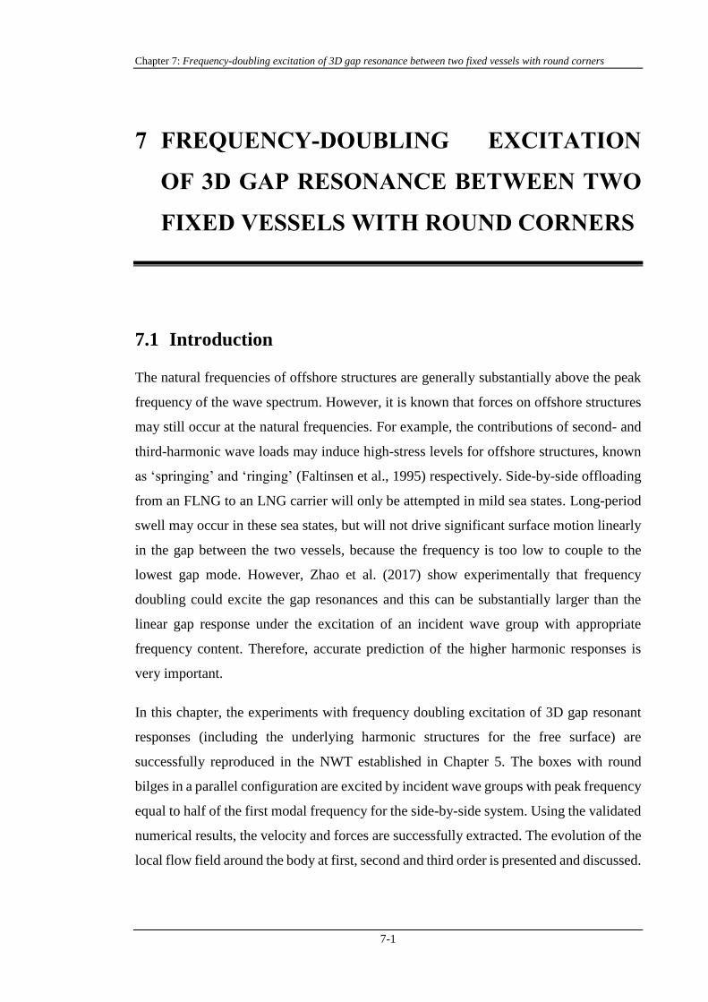
Figure 7.1 Numerically recreated linear incident wave group compared to experimental
results.
(a) time series
(b) amplitude spectrum
(c) phase spectrum
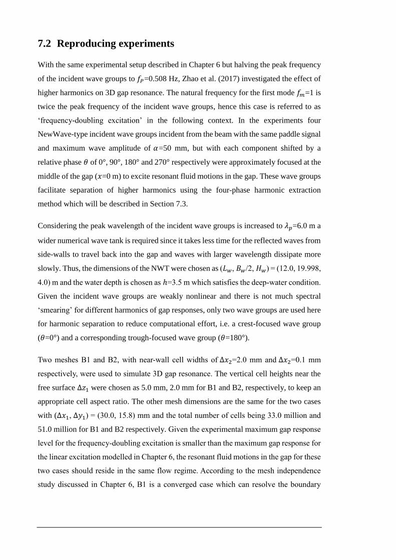
Figure 7.2 Numerically recreated crest-focused total incident wave group compared to
experimental results.
Chapter 7: Frequency-doubling excitation of 3D gap resonance between two fixed vessels with round corners
7-5
(a) time series
(b) amplitude spectrum
(c) phase spectrum
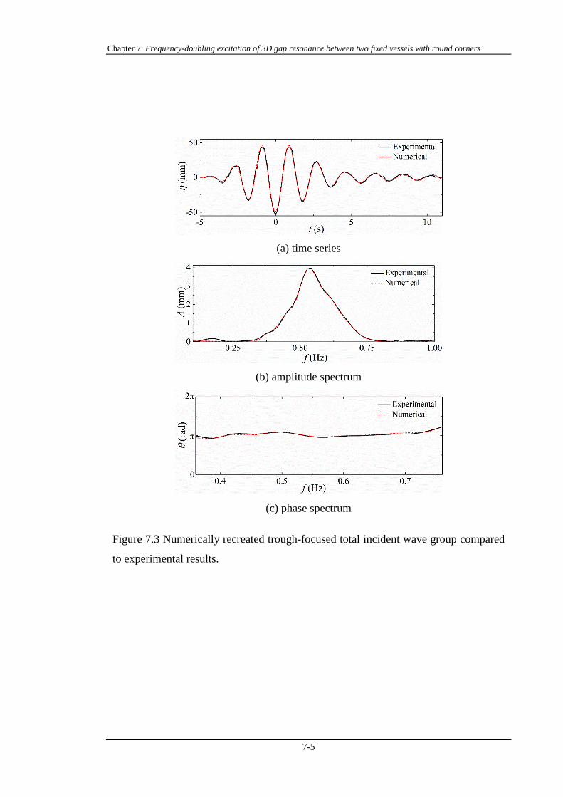
Figure 7.3 Numerically recreated trough-focused total incident wave group compared
to experimental results.
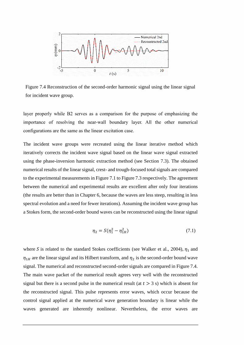
Figure 7.4 Reconstruction of the second-order harmonic signal using the linear signal
for incident wave group.
layer properly while B2 serves as a comparison for the purpose of emphasizing the
importance of resolving the near-wall boundary layer. All the other numerical
configurations are the same as the linear excitation case.
The incident wave groups were recreated using the linear iterative method which
iteratively corrects the incident wave signal based on the linear wave signal extracted
using the phase-inversion harmonic extraction method (see Section 7.3). The obtained
numerical results of the linear signal, crest- and trough-focused total signals are compared
to the experimental measurements in Figure 7.1 to Figure 7.3 respectively. The agreement
between the numerical and experimental results are excellent after only four iterations
(the results are better than in Chapter 6, because the waves are less steep, resulting in less
spectral evolution and a need for fewer iterations). Assuming the incident wave group has
a Stokes form, the second-order bound waves can be reconstructed using the linear signal
𝜂2 = 𝑆(𝜂12 − 𝜂1𝐻
2 ) (7.1)
where 𝑆 is related to the standard Stokes coefficients (see Walker et al., 2004), 𝜂1 and
𝜂1𝐻 are the linear signal and its Hilbert transform, and 𝜂2 is the second-order bound wave
signal. The numerical and reconstructed second-order signals are compared in Figure 7.4.
The main wave packet of the numerical result agrees very well with the reconstructed
signal but there is a second pulse in the numerical result (at 𝑡 > 3 s) which is absent for
the reconstructed signal. This pulse represents error waves, which occur because the
control signal applied at the numerical wave generation boundary is linear while the
waves generated are inherently nonlinear. Nevertheless, the error waves are
Chapter 7: Frequency-doubling excitation of 3D gap resonance between two fixed vessels with round corners
7-7
(a) Crest-focused total gap response
(b) Trough-focused total gap response
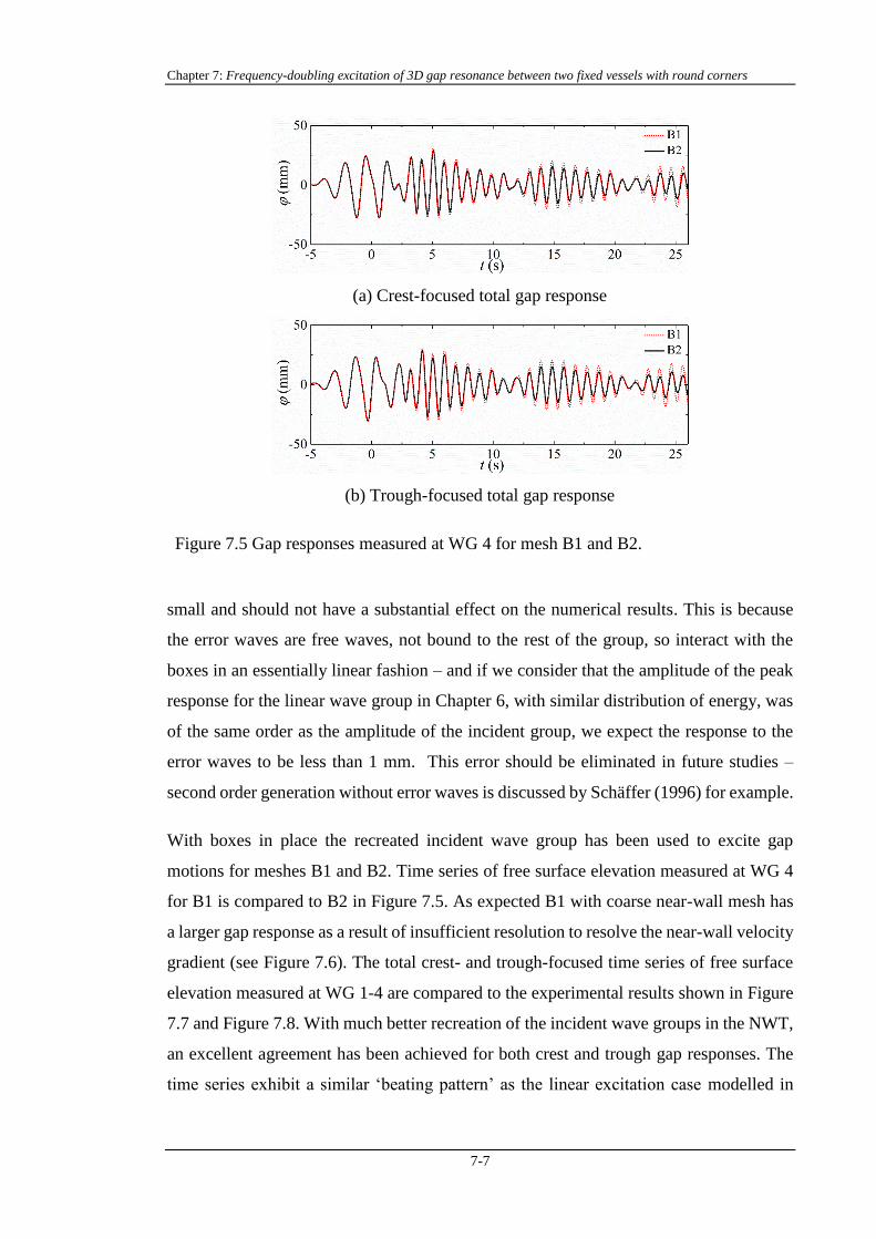
Figure 7.5 Gap responses measured at WG 4 for mesh B1 and B2.
small and should not have a substantial effect on the numerical results. This is because
the error waves are free waves, not bound to the rest of the group, so interact with the
boxes in an essentially linear fashion – and if we consider that the amplitude of the peak
response for the linear wave group in Chapter 6, with similar distribution of energy, was
of the same order as the amplitude of the incident group, we expect the response to the
error waves to be less than 1 mm. This error should be eliminated in future studies –
second order generation without error waves is discussed by Schäffer (1996) for example.
With boxes in place the recreated incident wave group has been used to excite gap
motions for meshes B1 and B2. Time series of free surface elevation measured at WG 4
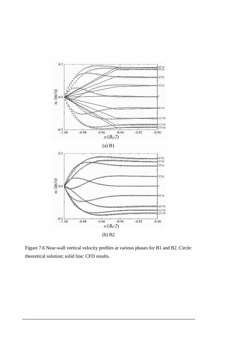
for B1 is compared to B2 in Figure 7.5. As expected B1 with coarse near-wall mesh has
a larger gap response as a result of insufficient resolution to resolve the near-wall velocity
gradient (see Figure 7.6). The total crest- and trough-focused time series of free surface
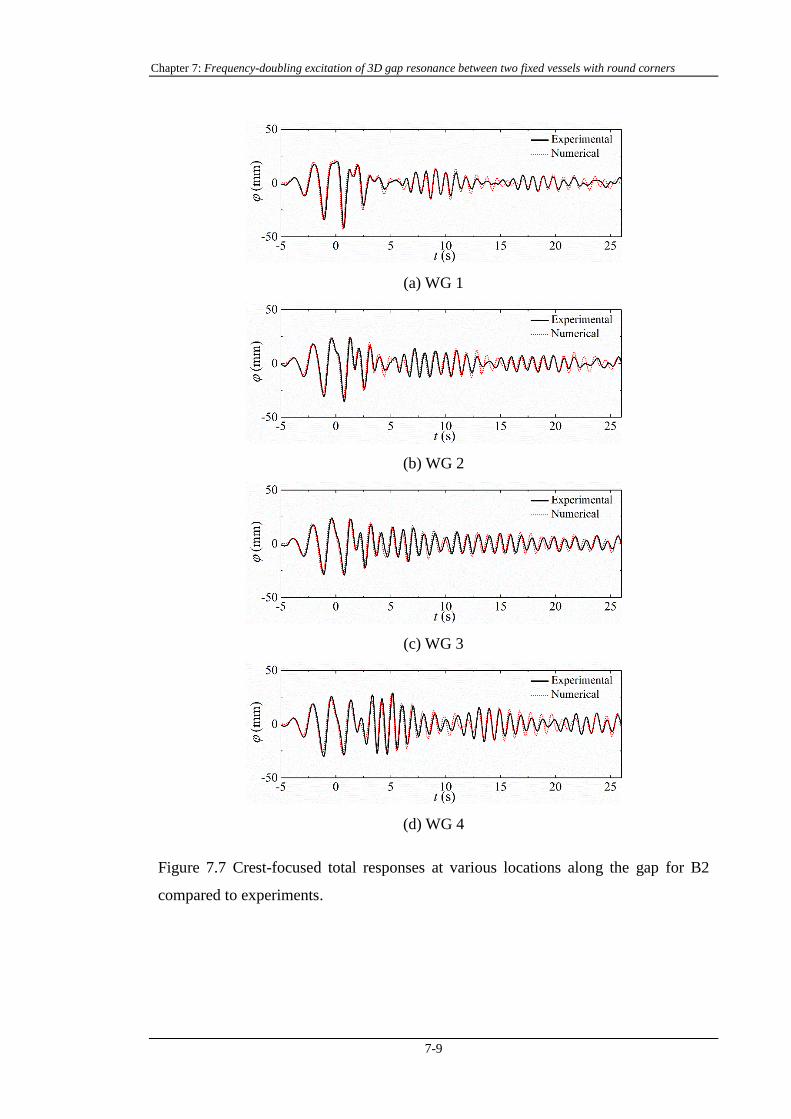
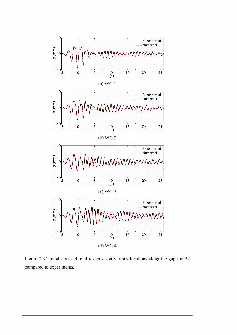
elevation measured at WG 1-4 are compared to the experimental results shown in Figure
7.7 and Figure 7.8. With much better recreation of the incident wave groups in the NWT,
an excellent agreement has been achieved for both crest and trough gap responses. The
time series exhibit a similar ‘beating pattern’ as the linear excitation case modelled in
(a) B1
(b) B2
Figure 7.6 Near-wall vertical velocity profiles at various phases for B1 and B2. Circle:
theoretical solution; solid line: CFD results.
Chapter 7: Frequency-doubling excitation of 3D gap resonance between two fixed vessels with round corners
7-9
(a) WG 1
(b) WG 2
(c) WG 3
(d) WG 4
Figure 7.7 Crest-focused total responses at various locations along the gap for B2
compared to experiments.
(a) WG 1
(b) WG 2
(c) WG 3
(d) WG 4
Figure 7.8 Trough-focused total responses at various locations along the gap for B2
compared to experiments.
Chapter 7: Frequency-doubling excitation of 3D gap resonance between two fixed vessels with round corners
7-11
Chapter 6. At the beginning the free surface in the gap oscillates with the same frequency
as the incident waves. When the incident waves have passed the gap the free surface in
the gap starts to oscillate at higher frequencies, which are a superposition of multiple
resonant modes.
7.3 Harmonic extraction method
For weakly nonlinear waves and wave-structure interaction, a regular incident wave will
induce a surface elevation of the form (written here to the fourth order in linear component
𝐴):
𝜂(𝜃) = 𝜂11𝐴 cos(𝜃) + 𝜂20𝐴2 + 𝜂22𝐴
2 cos(2𝜃)
+ 𝜂31𝐴3 cos(𝜃) + 𝜂33𝐴
3 cos(3𝜃)
+ 𝜂40𝐴4 + 𝜂42𝐴
4 cos(2𝜃) + 𝜂44𝐴4 cos(4𝜃) + 𝑂(𝐴5)
(7.2)
where 𝜃 is the phase function of the incident wave, and the coefficients 𝜂𝑖𝑗 represent
transfer functions between the incident surface elevation and response surface elevation
(with 𝑖 and 𝑗 standing for the power of amplitude and the frequency harmonic,
respectively). Separation of higher harmonics for response surface elevation induced by
a regular wave is straightforward using digital filtering, however, it is more complicated
for response surface elevation induced by wave groups where there is often overlap
between different harmonic contents.
To separate the odd and even harmonics of the response free surface elevation arising
from focused incident wave groups, the phase-inversion method applied to wave
kinematics described by Hunt et al. (2002) can be used. This method requires two time
series of a given hydrodynamic quantity induced by two incident waves that are 180° out
of phase. According to Eq. (7.2), when the phase function is shifted from 𝜃 to 𝜃 + 𝜋 the
signs of the odd harmonics will be inverted while the signs of the even harmonics will
remain the same. Therefore, the odd and even harmonics are separated by taking the
averaged difference and sum of the free surface elevation signals, respectively,
𝜂0 − 𝜂1802
= (𝜂11𝐴 + 𝜂31𝐴3) cos(𝜃) + 𝜂33𝐴
3 cos(3𝜃) + 𝑂(𝐴5) (7.3)
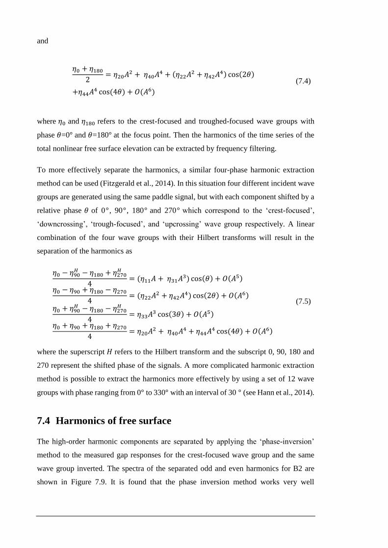
and
𝜂0 + 𝜂1802
= 𝜂20𝐴2 + 𝜂40𝐴
4 + (𝜂22𝐴2 + 𝜂42𝐴
4) cos(2𝜃)
+𝜂44𝐴4 cos(4𝜃) + 𝑂(𝐴6)
(7.4)
where 𝜂0 and 𝜂180 refers to the crest-focused and troughed-focused wave groups with
phase 𝜃=0° and 𝜃=180° at the focus point. Then the harmonics of the time series of the
total nonlinear free surface elevation can be extracted by frequency filtering.
To more effectively separate the harmonics, a similar four-phase harmonic extraction
method can be used (Fitzgerald et al., 2014). In this situation four different incident wave
groups are generated using the same paddle signal, but with each component shifted by a
relative phase 𝜃 of 0° , 90°, 180° and 270° which correspond to the ‘crest-focused’,
‘downcrossing’, ‘trough-focused’, and ‘upcrossing’ wave group respectively. A linear
combination of the four wave groups with their Hilbert transforms will result in the
separation of the harmonics as
𝜂0 − 𝜂90𝐻 − 𝜂180 + 𝜂270
𝐻
4= (𝜂11𝐴 + 𝜂31𝐴
3) cos(𝜃) + 𝑂(𝐴5)
𝜂0 − 𝜂90 + 𝜂180 − 𝜂2704
= (𝜂22𝐴2 + 𝜂42𝐴
4) cos(2𝜃) + 𝑂(𝐴6)
𝜂0 + 𝜂90𝐻 − 𝜂180 − 𝜂270
𝐻
4= 𝜂33𝐴
3 cos(3𝜃) + 𝑂(𝐴5)
𝜂0 + 𝜂90 + 𝜂180 + 𝜂2704
= 𝜂20𝐴2 + 𝜂40𝐴
4 + 𝜂44𝐴4 cos(4𝜃) + 𝑂(𝐴6)
(7.5)
where the superscript 𝐻 refers to the Hilbert transform and the subscript 0, 90, 180 and
270 represent the shifted phase of the signals. A more complicated harmonic extraction
method is possible to extract the harmonics more effectively by using a set of 12 wave
groups with phase ranging from 0° to 330° with an interval of 30 ° (see Hann et al., 2014).
7.4 Harmonics of free surface
The high-order harmonic components are separated by applying the ‘phase-inversion’
method to the measured gap responses for the crest-focused wave group and the same
wave group inverted. The spectra of the separated odd and even harmonics for B2 are
shown in Figure 7.9. It is found that the phase inversion method works very well
Chapter 7: Frequency-doubling excitation of 3D gap resonance between two fixed vessels with round corners
7-13
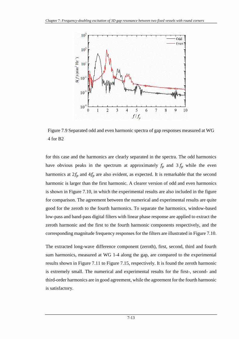
Figure 7.9 Separated odd and even harmonic spectra of gap responses measured at WG
4 for B2
for this case and the harmonics are clearly separated in the spectra. The odd harmonics
have obvious peaks in the spectrum at approximately 𝑓𝑝 and 3 𝑓𝑝 while the even
harmonics at 2𝑓𝑝 and 4𝑓𝑝 are also evident, as expected. It is remarkable that the second
harmonic is larger than the first harmonic. A clearer version of odd and even harmonics
is shown in Figure 7.10, in which the experimental results are also included in the figure
for comparison. The agreement between the numerical and experimental results are quite
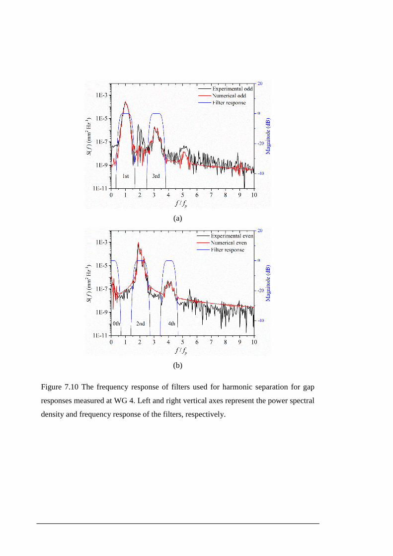
good for the zeroth to the fourth harmonics. To separate the harmonics, window-based
low-pass and band-pass digital filters with linear phase response are applied to extract the
zeroth harmonic and the first to the fourth harmonic components respectively, and the
corresponding magnitude frequency responses for the filters are illustrated in Figure 7.10.
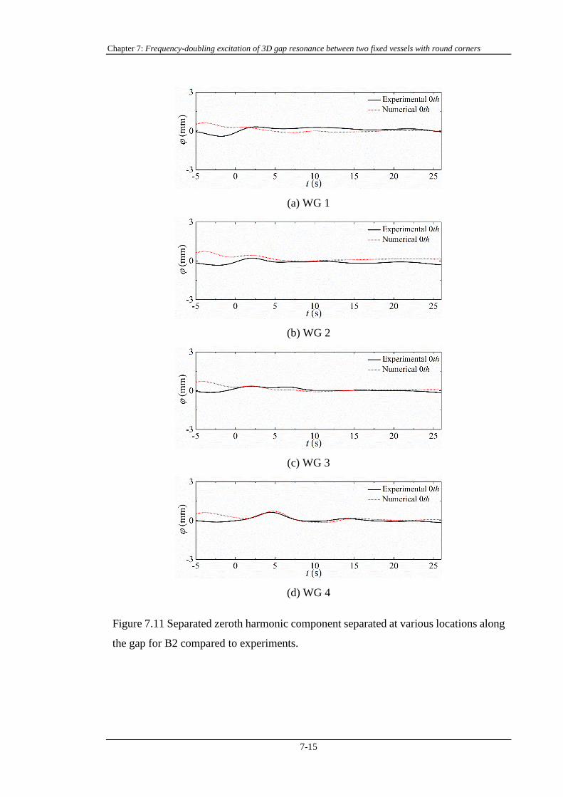
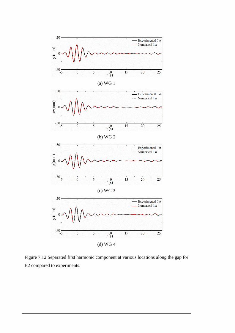
The extracted long-wave difference component (zeroth), first, second, third and fourth
sum harmonics, measured at WG 1-4 along the gap, are compared to the experimental
results shown in Figure 7.11 to Figure 7.15, respectively. It is found the zeroth harmonic
is extremely small. The numerical and experimental results for the first-, second- and
third-order harmonics are in good agreement, while the agreement for the fourth harmonic
is satisfactory.
(a)
(b)
Figure 7.10 The frequency response of filters used for harmonic separation for gap
responses measured at WG 4. Left and right vertical axes represent the power spectral
density and frequency response of the filters, respectively.
Chapter 7: Frequency-doubling excitation of 3D gap resonance between two fixed vessels with round corners
7-15
(a) WG 1
(b) WG 2
(c) WG 3
(d) WG 4
Figure 7.11 Separated zeroth harmonic component separated at various locations along
the gap for B2 compared to experiments.
(a) WG 1
(b) WG 2
(c) WG 3
(d) WG 4
Figure 7.12 Separated first harmonic component at various locations along the gap for
B2 compared to experiments.
Chapter 7: Frequency-doubling excitation of 3D gap resonance between two fixed vessels with round corners
7-17
(a) WG 1
(b) WG 2
(c) WG 3
(d) WG 4
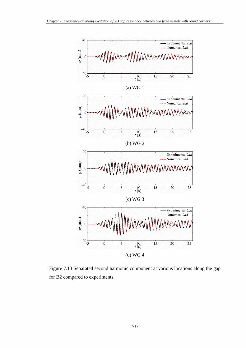
Figure 7.13 Separated second harmonic component at various locations along the gap
for B2 compared to experiments.
(a) WG 1
(b) WG 2
(c) WG 3
(d) WG 4
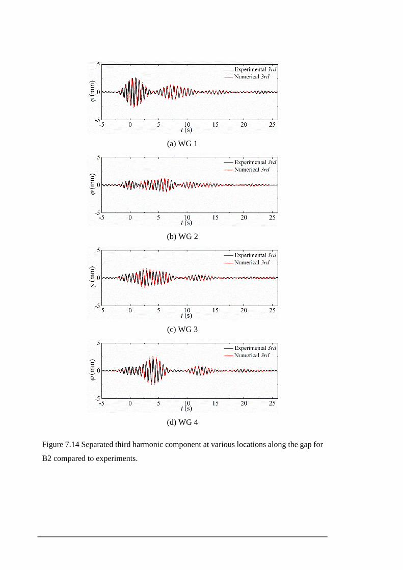
Figure 7.14 Separated third harmonic component at various locations along the gap for
B2 compared to experiments.
Chapter 7: Frequency-doubling excitation of 3D gap resonance between two fixed vessels with round corners
7-19
(a) WG 1
(b) WG 2
(c) WG 3
(d) WG 4
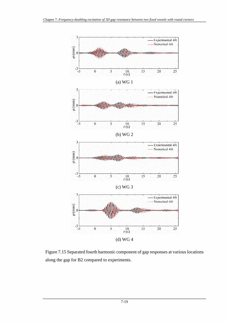
Figure 7.15 Separated fourth harmonic component of gap responses at various locations
along the gap for B2 compared to experiments.
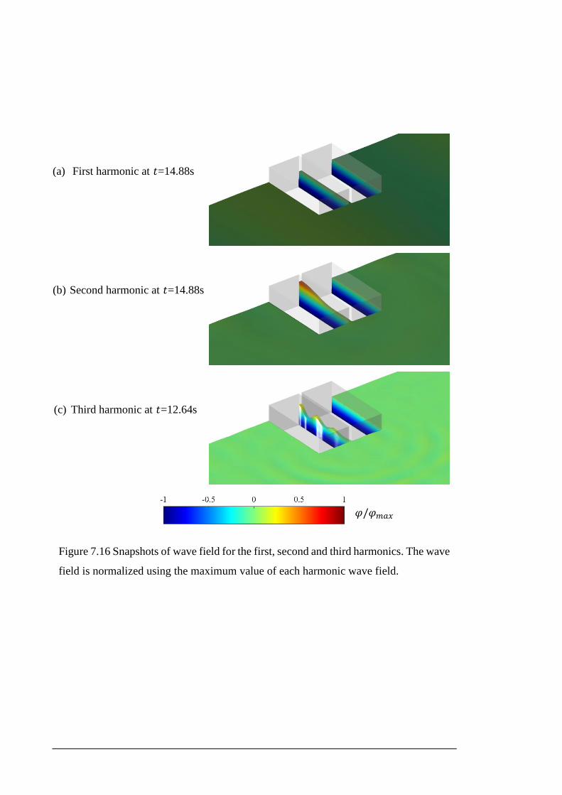
Figure 7.16 Snapshots of wave field for the first, second and third harmonics. The wave
field is normalized using the maximum value of each harmonic wave field.
𝜑/𝜑𝑚𝑎𝑥
(a) First harmonic at 𝑡=14.88s
(b) Second harmonic at 𝑡=14.88s
(c) Third harmonic at 𝑡=12.64s
Chapter 7: Frequency-doubling excitation of 3D gap resonance between two fixed vessels with round corners
7-21
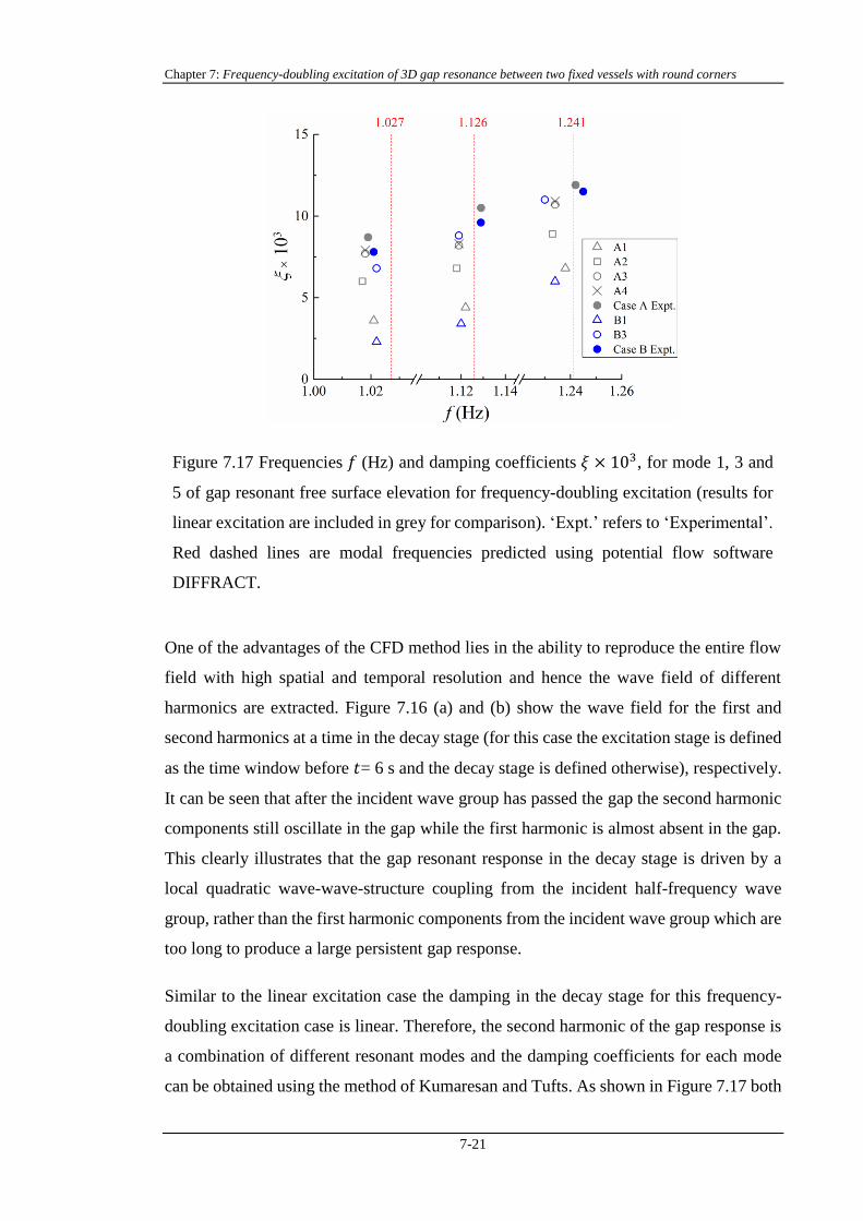
Figure 7.17 Frequencies 𝑓 (Hz) and damping coefficients 𝜉 × 103, for mode 1, 3 and
5 of gap resonant free surface elevation for frequency-doubling excitation (results for
linear excitation are included in grey for comparison). ‘Expt.’ refers to ‘Experimental’.
Red dashed lines are modal frequencies predicted using potential flow software
DIFFRACT.
One of the advantages of the CFD method lies in the ability to reproduce the entire flow
field with high spatial and temporal resolution and hence the wave field of different
harmonics are extracted. Figure 7.16 (a) and (b) show the wave field for the first and
second harmonics at a time in the decay stage (for this case the excitation stage is defined
as the time window before 𝑡= 6 s and the decay stage is defined otherwise), respectively.
It can be seen that after the incident wave group has passed the gap the second harmonic
components still oscillate in the gap while the first harmonic is almost absent in the gap.
This clearly illustrates that the gap resonant response in the decay stage is driven by a
local quadratic wave-wave-structure coupling from the incident half-frequency wave
group, rather than the first harmonic components from the incident wave group which are
too long to produce a large persistent gap response.
Similar to the linear excitation case the damping in the decay stage for this frequency-
doubling excitation case is linear. Therefore, the second harmonic of the gap response is
a combination of different resonant modes and the damping coefficients for each mode
can be obtained using the method of Kumaresan and Tufts. As shown in Figure 7.17 both
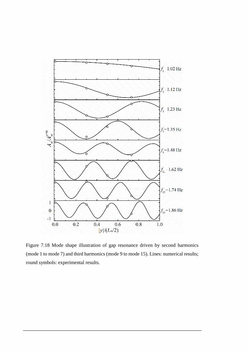
Figure 7.18 Mode shape illustration of gap resonance driven by second harmonics
(mode 1 to mode 7) and third harmonics (mode 9 to mode 15). Lines: numerical results;
round symbols: experimental results.
Chapter 7: Frequency-doubling excitation of 3D gap resonance between two fixed vessels with round corners
7-23
(a) WG 1
(b) WG 2
(c) WG 3
(d) WG 4
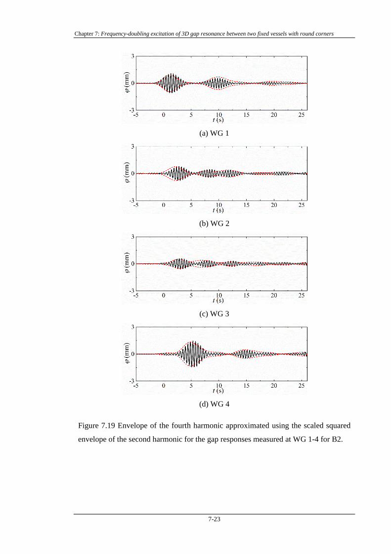
Figure 7.19 Envelope of the fourth harmonic approximated using the scaled squared
envelope of the second harmonic for the gap responses measured at WG 1-4 for B2.
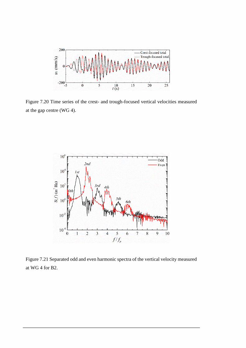
Figure 7.20 Time series of the crest- and trough-focused vertical velocities measured
at the gap centre (WG 4).
Figure 7.21 Separated odd and even harmonic spectra of the vertical velocity measured
at WG 4 for B2.
Chapter 7: Frequency-doubling excitation of 3D gap resonance between two fixed vessels with round corners
7-25
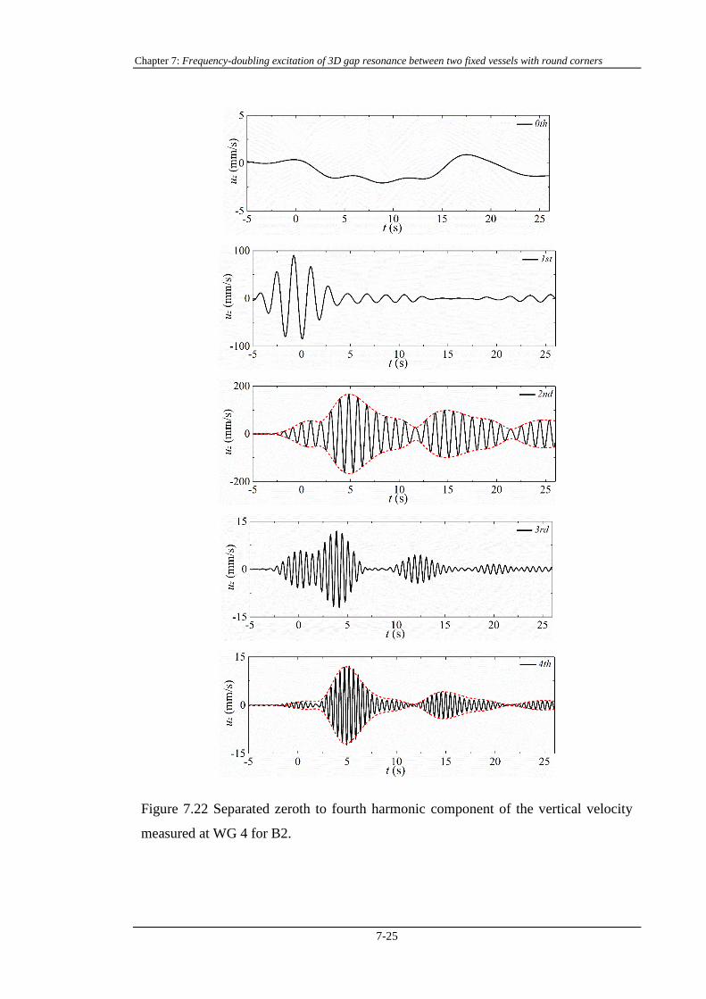
Figure 7.22 Separated zeroth to fourth harmonic component of the vertical velocity
measured at WG 4 for B2.
the numerical results obtained from CFD and potential flow models give an excellent
prediction of the resonant frequencies for each mode. In terms of damping coefficients,
B1 with coarse near-wall mesh clearly underpredicts the experiment. When the near-wall
mesh is refined, it can be seen the damping coefficients for B2 agree well with the
experimental results although there is still some underprediction. These results are
consistent with the linear excitation case.
Similar to the second harmonic wave field, obvious standing waves are found in the gap
for the third harmonic wave field (see the normalized third harmonic in the decay stage
in Figure 7.16 (c)). The first to the fifteenth mode shapes with corresponding resonant
frequencies are shown in Figure 7.18, in which the first to the seventh mode shapes are
identified from the second harmonic while the ninth to the fifteenth mode shapes from
the third harmonic. It is found the numerical results give excellent agreement with the
experimental results.
Given there is a generalized Stokes type perturbation expansion for the gap responses, it
is possible to approximate the envelope of the 𝑛th harmonic component by raising the
fundamental envelope (calculated as in Section 4.2.1) to the power 𝑛 and then fitting the
measured envelope of the 𝑛th harmonic component by a least-square method. Figure 7.19
shows the envelope of the fourth harmonic component approximated using the envelope
of the second harmonic component which is calculated by using the Hilbert transform. It
is found that the extracted fourth harmonic fits the scaled squared envelopes of the second
harmonic quite well. This means the numerical results are self-consistent in that the fourth
harmonic component is bound to the second harmonic component, although some
discrepancies between the numerical and experimental results are found for the fourth
harmonic.
To summarize, these numerical results for the free surface elevations in the gap give a
very good prediction of the experiment. This gives us the confidence to analyse other
quantities in detail, such as the velocity and hydrodynamic force on the boxes which will
be discussed in the following sections.
7.5 Harmonics of velocity
The time series of the crest- and trough-focused vertical velocities measured at the gap
centre in the mid-ship plane are shown in Figure 7.20. The sampling point is located at
0.08 m vertically below the mean free surface which always stays wet. It can be identified
Chapter 7: Frequency-doubling excitation of 3D gap resonance between two fixed vessels with round corners
7-27
from the time series that the odd harmonics dominate the excitation stage while the even
harmonics dominate the decay stage. Using the phase-inversion method, harmonic
structures up to the sixth can be identified in the power spectra shown in Figure 7.21. It
is remarkable that the second harmonic component is much larger than the first harmonic
component.
By digital filtering, the time series of the zeroth to the fourth harmonic are shown in
Figure 7.22. The fifth and sixth harmonics (with a maximum amplitude smaller than 2.0
mm/s and 1.4 mm/s) are very small and are not shown here. From the results it is seen
that for the vertical velocity the maximum amplitude of the second harmonic component
is 1.85 times that of the first harmonic component, whereas the ratio for the free surface
elevation is approximately 1. The envelopes for the fourth harmonic component are
obtained as the scaled squared envelopes for the second harmonic component, through a
least squares numerical fit method. The fitted envelope matches the time series of the
fourth harmonic component remarkably well, showing how the fourth harmonic ‘follows’
the second harmonic.
7.6 Harmonics of hydrodynamic force
Wave loading on offloading vessels is the major external force to be considered in the
design stage of offloading operability. Hydrodynamic forces induced by external waves
have a critical effect on the relative motions of the offloading vessels. Using the validated
results from B2 the hydrodynamic forces are obtained by integrating the pressure over
the time-varying wet surface of the boxes. Due to the symmetry condition in the mid-ship
plane only horizontal forces along the wave propagation direction 𝐹𝑥 and vertical forces
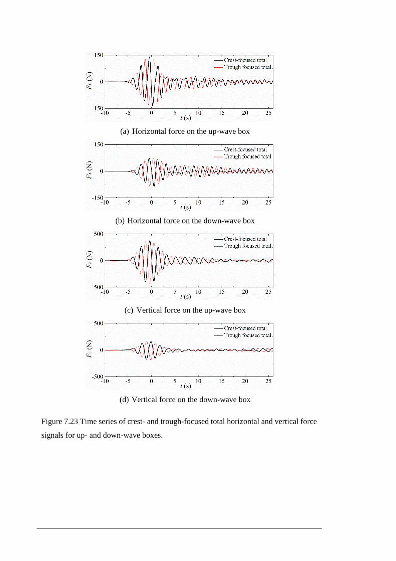
𝐹𝑧 are present. Figure 7.23 shows the time histories of the total horizontal and vertical
forces on the up- and down-wave boxes for a crest-focused wave group and the same
wave group inverted. It is evident that the up-wave box ‘shields’ the down-wave box in
the excitation stage – the maximum horizontal and vertical forces for the up-wave box
are 47% and 58% larger than the counterparts for the down-wave box respectively. The
vertical forces are at least two times larger than the horizontal forces.
By applying the phase-inversion method using the crest- and trough- focused forces, the
odd and even harmonics are obtained. The power spectra of the odd and even harmonics
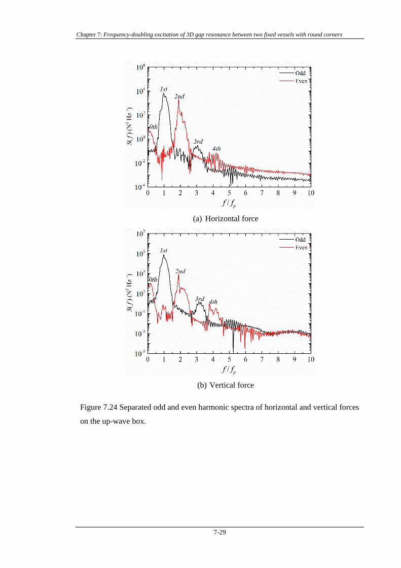
for the horizontal and vertical forces are shown in Figure 7.24, where the harmonics are
(a) Horizontal force on the up-wave box
(b) Horizontal force on the down-wave box
(c) Vertical force on the up-wave box
(d) Vertical force on the down-wave box
Figure 7.23 Time series of crest- and trough-focused total horizontal and vertical force
signals for up- and down-wave boxes.
Chapter 7: Frequency-doubling excitation of 3D gap resonance between two fixed vessels with round corners
7-29
(a) Horizontal force
(b) Vertical force
Figure 7.24 Separated odd and even harmonic spectra of horizontal and vertical forces
on the up-wave box.
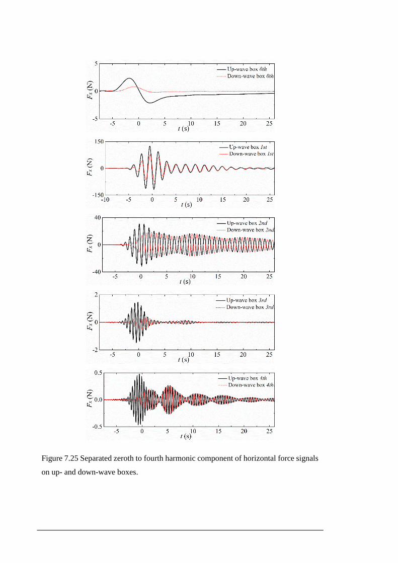
Figure 7.25 Separated zeroth to fourth harmonic component of horizontal force signals
on up- and down-wave boxes.
Chapter 7: Frequency-doubling excitation of 3D gap resonance between two fixed vessels with round corners
7-31
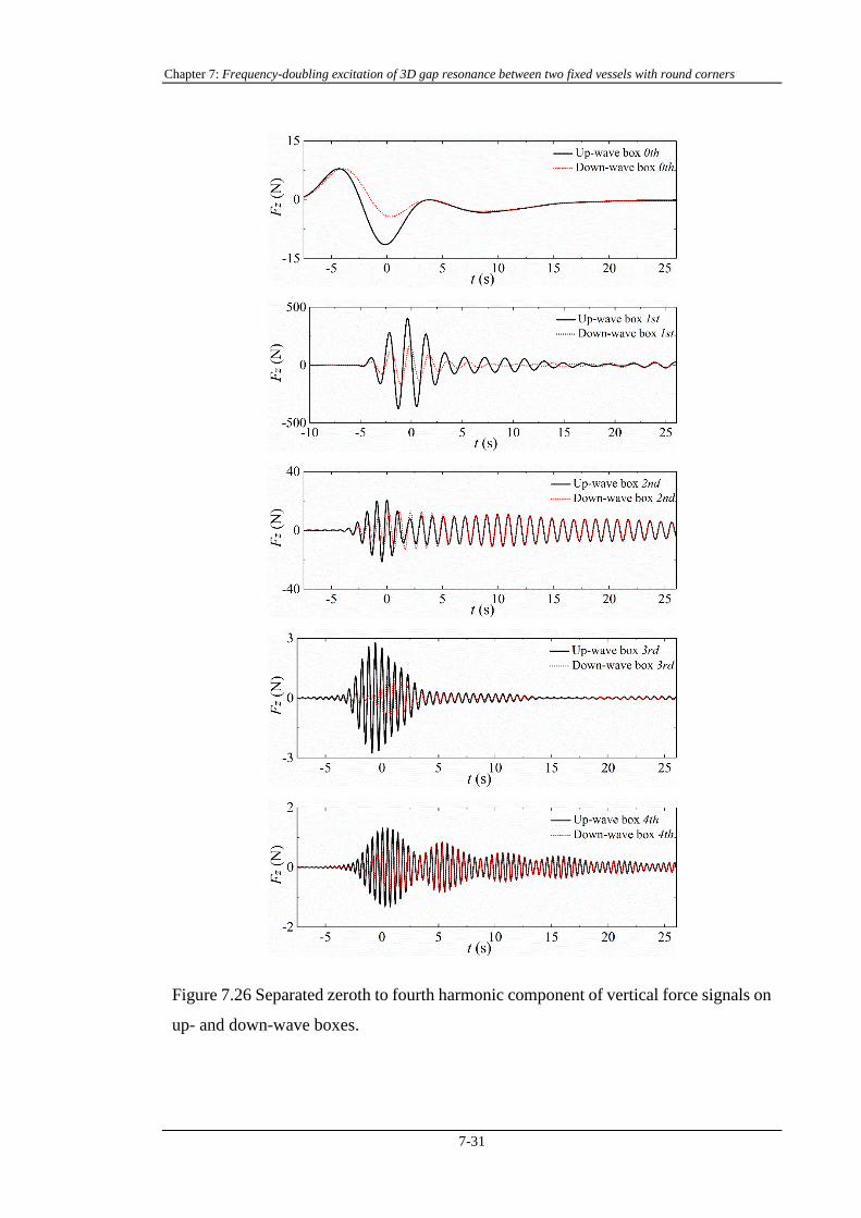
Figure 7.26 Separated zeroth to fourth harmonic component of vertical force signals on
up- and down-wave boxes.
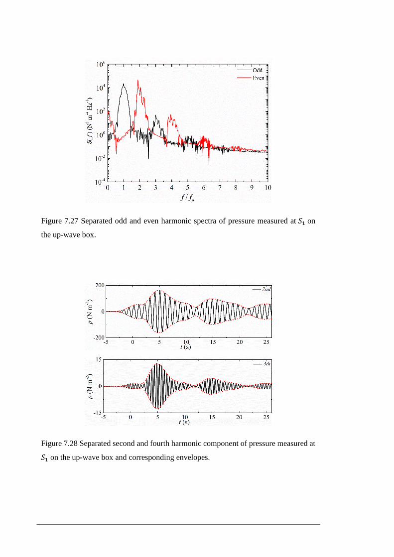
Figure 7.27 Separated odd and even harmonic spectra of pressure measured at 𝑆1 on
the up-wave box.
Figure 7.28 Separated second and fourth harmonic component of pressure measured at
𝑆1 on the up-wave box and corresponding envelopes.
Chapter 7: Frequency-doubling excitation of 3D gap resonance between two fixed vessels with round corners
7-33
well separated. The zeroth to the fourth harmonic components for horizontal and vertical
forces are shown in Figure 7.25 and Figure 7.26 respectively, where the forces on the up-
and down-wave boxes are compared in each subfigure. The shielding effect from the up-
wave box is most significant in the excitation stage due to the large incident wave loading.
In this stage the first harmonic is dominant, and the second harmonic is much smaller.
When the incident wave group has passed the second harmonic becomes more important.
This is more pronounced for the horizontal force, where the second harmonic can become
larger than the first harmonic over time owing to the very small radiation damping for the
second harmonic. This suggests that in a random sea of this amplitude, the maximum first
and second-order horizontal forces may be comparable in magnitude, since the present
wave group produces a force which is close to a NewWave in shape, while the second-
order force is quite different. It should also be noted that one of the original motivations
for developing ‘lid’ methods was the excessive mean force predictions of potential flow
codes (e.g. Buchner et al., 2001). There is no such issue here, where the low-frequency
forces are quite modest.
For the hydrodynamic forces on the boxes the scaled squared envelopes for the second
harmonic cannot match the time series for the fourth harmonic. This is because the
hydrodynamic forces on the boxes are determined by the flow in the gap and outside the
gap, and also affected by the time-varying free surface elevation. For example, the
contributions for the second harmonic are associated partly with second-order pressure
acting on the mean submerged surface of the boxes, and also with the effect of the first-
order pressure acting on the time-varying boundary at the free surface. To further confirm
this the harmonic structures for the pressure measured at a point on the up-wave box in
the gap 𝑆1 (–𝐵𝑔/2, 0, -0.08) m are checked. The harmonic spectra, and the second and
fourth harmonics with corresponding envelopes are shown in Figure 7.27 and Figure 7.28
respectively. Remarkably good agreement between the scaled squared envelopes of the
second harmonic component and the time series of the fourth harmonic component is
achieved, as expected.
7.7 Conclusions
In this chapter the numerical results of harmonic structures including the zeroth, first,
second and third harmonics for free surface elevation show excellent agreement with
experimental results. Using the validated numerical results, the higher harmonics for the
velocity and the hydrodynamic forces on the boxes are also successfully extracted. This
represents a highly successful application of CFD to a problem with linear viscous
dissipation but nonlinear free surface effects, both of which must be resolved to achieve
satisfactory results. CFD has previously been used to derive second harmonic responses
around non-resonant structures such as cylinders in relatively steep waves (Paulsen et al.,
2014). Here the strength of the second harmonic response is much stronger (so more
challenging to simulate correctly); even in waves which are not steep the second harmonic
responses are as large as the first. Given the success of reproducing higher harmonics
using the CFD method, it is expected that even higher harmonics could be well predicted
if the mesh resolution near the free surface was further refined, though their practical
significance may be limited. However, quadratic excitation of gap resonance does appear
to be a problem of practical relevance.
Significant shielding effect from the up-wave box is observed in the excitation stage, such
that the wave loading on the up-wave box can be up to 58% larger than the down-wave
box. In practical offloading scenarios, it may be preferable to arrange the LNG carrier on
the down-wave side (if it is not achievable to align the vessels parallel to the direction of
the predominant environmental forces) since its motions are more sensitive to large
hydrodynamic forces compared to the FLNG.
Chapter 8: 3D gap resonance between two fixed vessels with square corners
8-1
8 3D GAP RESONANCE BETWEEN TWO
FIXED VESSELS WITH SQUARE CORNERS
8.1 Introduction
According to the discussion in Chapter 4, the flow features and wave responses for 2D
gap resonance are distinct for round and square entrance shapes. For square entrance
shapes, flow separation will occur around the sharp corners. Zhao et al (2017) also
conducted a series of wave basin tests with models with square corners. In this chapter,
the experimental results of 3D gap resonance with square corners under the excitation of
transient groups are first presented, and then the experimental gap responses are
reproduced in the NWT. The numerical and experimental results differ by more than in
the round corner case, and both the resonant frequencies and damping coefficients are
overpredicted by the numerical model. Discussion is given concerning potential causes
of this difference which may prove useful for future study on this topic.
8.2 Physical setup
A series of experiments for 3D gap resonance in between vessels with square corners
were carried out in the State Key Laboratory of Ocean Engineering at Shanghai Jiao Tong
University by Zhao et al (2017). The vessel models used in the experiments are shown in
Figure 8.1, where bespoke strips were stuck on to the round corners of the boxes (which
were used in the previous experiments described in Chapter 5) to form square corners.
Otherwise, the configuration is similar to that for the boxes with round corners. The main
dimensions of the boxes are (𝐿𝑚, 𝐵𝑚, 𝐻𝑚, 𝐷𝑚)= (3.333, 0.767, 0.425, 0.185) m, where
𝐿𝑚, 𝐵𝑚, 𝐻𝑚 and 𝐷𝑚 are the length, width, height and draft of the model, respectively.
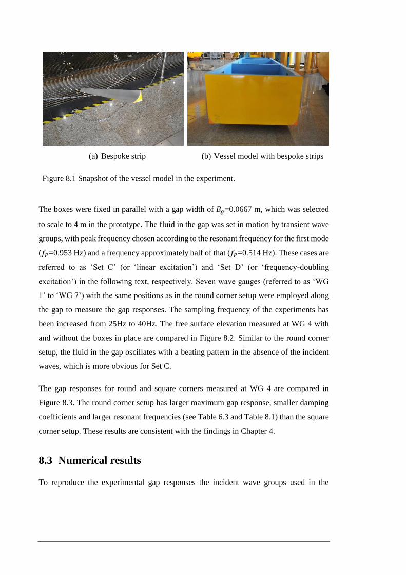
(a) Bespoke strip (b) Vessel model with bespoke strips
Figure 8.1 Snapshot of the vessel model in the experiment.
The boxes were fixed in parallel with a gap width of 𝐵𝑔=0.0667 m, which was selected
to scale to 4 m in the prototype. The fluid in the gap was set in motion by transient wave
groups, with peak frequency chosen according to the resonant frequency for the first mode
(𝑓𝑃=0.953 Hz) and a frequency approximately half of that (𝑓𝑃=0.514 Hz). These cases are
referred to as ‘Set C’ (or ‘linear excitation’) and ‘Set D’ (or ‘frequency-doubling
excitation’) in the following text, respectively. Seven wave gauges (referred to as ‘WG
1’ to ‘WG 7’) with the same positions as in the round corner setup were employed along
the gap to measure the gap responses. The sampling frequency of the experiments has
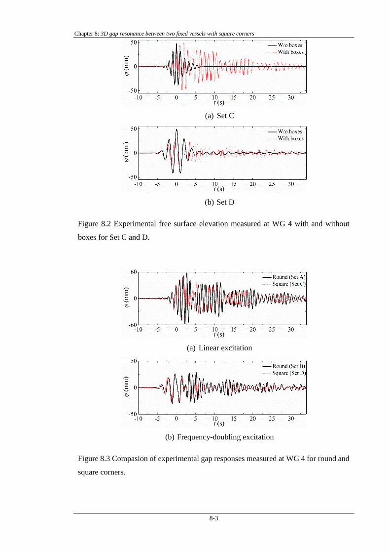
been increased from 25Hz to 40Hz. The free surface elevation measured at WG 4 with
and without the boxes in place are compared in Figure 8.2. Similar to the round corner
setup, the fluid in the gap oscillates with a beating pattern in the absence of the incident
waves, which is more obvious for Set C.
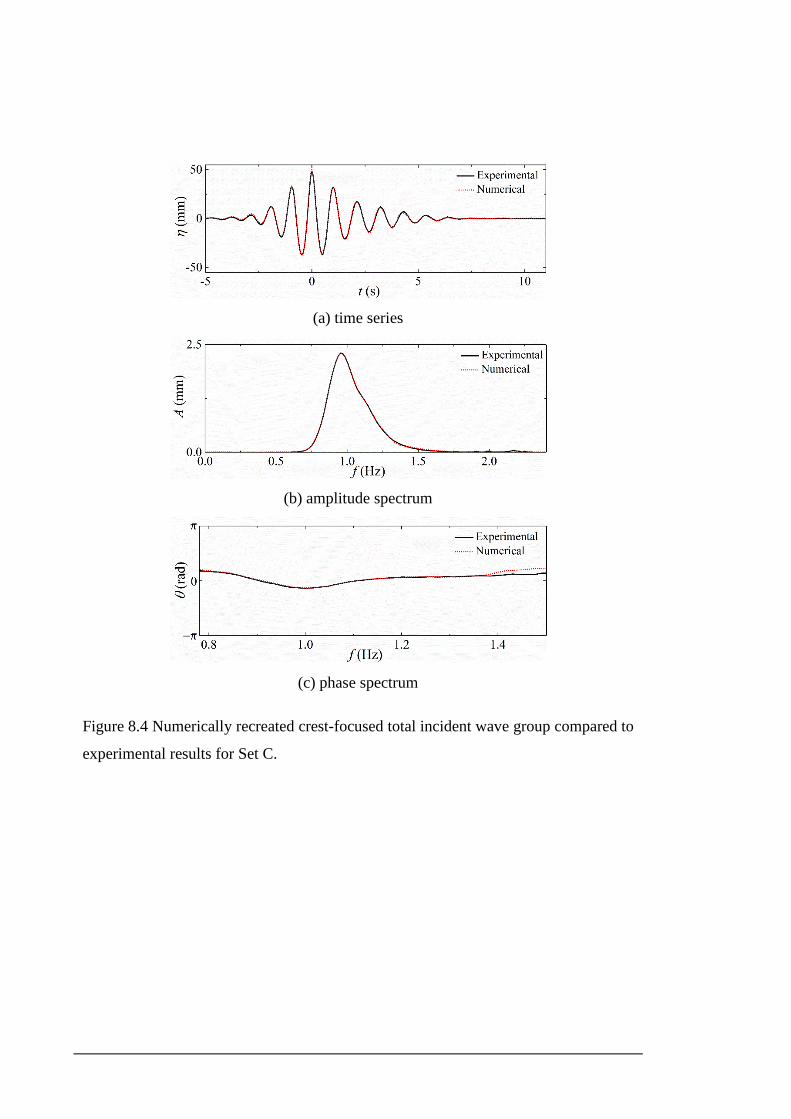
The gap responses for round and square corners measured at WG 4 are compared in
Figure 8.3. The round corner setup has larger maximum gap response, smaller damping
coefficients and larger resonant frequencies (see Table 6.3 and Table 8.1) than the square
corner setup. These results are consistent with the findings in Chapter 4.
8.3 Numerical results
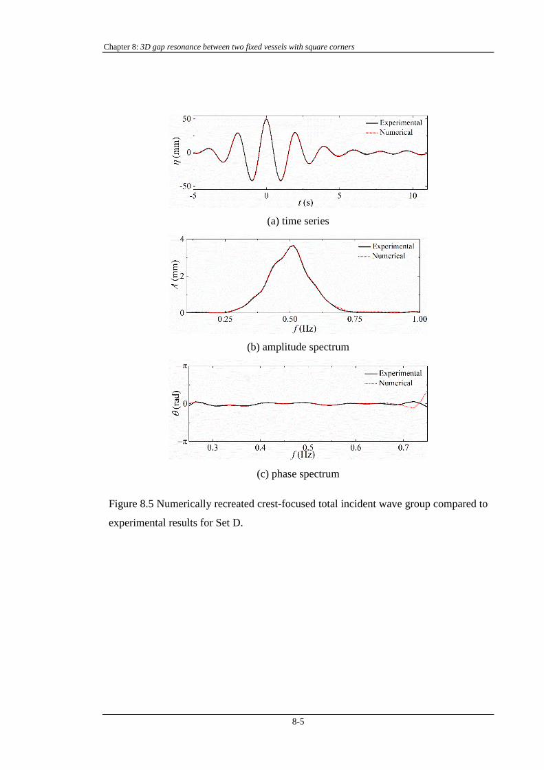
To reproduce the experimental gap responses the incident wave groups used in the
Chapter 8: 3D gap resonance between two fixed vessels with square corners
8-3
(a) Set C
(b) Set D
Figure 8.2 Experimental free surface elevation measured at WG 4 with and without
boxes for Set C and D.
(a) Linear excitation
(b) Frequency-doubling excitation
Figure 8.3 Compasion of experimental gap responses measured at WG 4 for round and
square corners.
(a) time series
(b) amplitude spectrum
(c) phase spectrum
Figure 8.4 Numerically recreated crest-focused total incident wave group compared to
experimental results for Set C.
Chapter 8: 3D gap resonance between two fixed vessels with square corners
8-5
(a) time series
(b) amplitude spectrum
(c) phase spectrum
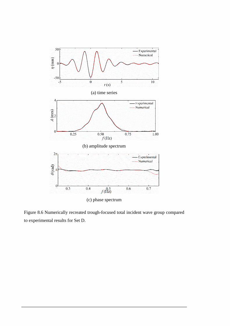
Figure 8.5 Numerically recreated crest-focused total incident wave group compared to
experimental results for Set D.
(a) time series
(b) amplitude spectrum
(c) phase spectrum
Figure 8.6 Numerically recreated trough-focused total incident wave group compared
to experimental results for Set D.
Chapter 8: 3D gap resonance between two fixed vessels with square corners
8-7
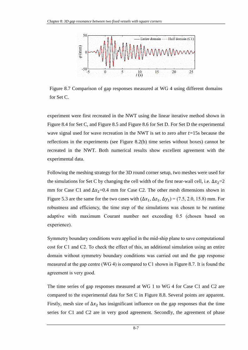
Figure 8.7 Comparison of gap responses measured at WG 4 using different domains
for Set C.
experiment were first recreated in the NWT using the linear iterative method shown in
Figure 8.4 for Set C, and Figure 8.5 and Figure 8.6 for Set D. For Set D the experimental
wave signal used for wave recreation in the NWT is set to zero after 𝑡=15s because the
reflections in the experiments (see Figure 8.2(b) time series without boxes) cannot be
recreated in the NWT. Both numerical results show excellent agreement with the
experimental data.
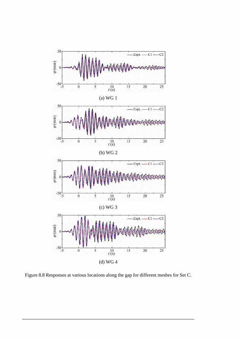
Following the meshing strategy for the 3D round corner setup, two meshes were used for
the simulations for Set C by changing the cell width of the first near-wall cell, i.e. Δ𝑥2=2
mm for Case C1 and Δ𝑥2=0.4 mm for Case C2. The other mesh dimensions shown in
Figure 5.3 are the same for the two cases with (Δ𝑥1, Δ𝑧1, Δ𝑦1) (7.5, 2.0, 15.8) mm. For
robustness and efficiency, the time step of the simulations was chosen to be runtime
adaptive with maximum Courant number not exceeding 0.5 (chosen based on
experience).
Symmetry boundary conditions were applied in the mid-ship plane to save computational
cost for C1 and C2. To check the effect of this, an additional simulation using an entire
domain without symmetry boundary conditions was carried out and the gap response
measured at the gap centre (WG 4) is compared to C1 shown in Figure 8.7. It is found the
agreement is very good.
The time series of gap responses measured at WG 1 to WG 4 for Case C1 and C2 are
compared to the experimental data for Set C in Figure 8.8. Several points are apparent.
Firstly, mesh size of Δ𝑥2 has insignificant influence on the gap responses that the time
series for C1 and C2 are in very good agreement. Secondly, the agreement of phase
(a) WG 1
(b) WG 2
(c) WG 3
(d) WG 4
Figure 8.8 Responses at various locations along the gap for different meshes for Set C.
Chapter 8: 3D gap resonance between two fixed vessels with square corners
8-9
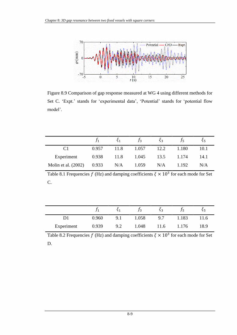
Figure 8.9 Comparison of gap response measured at WG 4 using different methods for
Set C. ‘Expt.’ stands for ‘experimental data’, ‘Potential’ stands for ‘potential flow
model’.
𝑓1 𝜉1 𝑓3 𝜉3 𝑓5 𝜉5
C1 0.957 11.8 1.057 12.2 1.180 10.1
Experiment 0.938 11.8 1.045 13.5 1.174 14.1
Molin et al. (2002) 0.933 N/A 1.059 N/A 1.192 N/A
Table 8.1 Frequencies 𝑓 (Hz) and damping coefficients 𝜉 × 103 for each mode for Set
C.
𝑓1 𝜉1 𝑓3 𝜉3 𝑓5 𝜉5
D1 0.960 9.1 1.058 9.7 1.183 11.6
Experiment 0.939 9.2 1.048 11.6 1.176 18.9
Table 8.2 Frequencies 𝑓 (Hz) and damping coefficients 𝜉 × 103 for each mode for Set
D.
between CFD and experimental results is very good for the first pulse in the excitation
stage (𝑡 < 5 s). After that, the CFD results begin to lead in phase, with accumulation over
time. At the end of the time window in the figure, the experimental and CFD results are
approximately 180 ° out of phase. For comparison, the time series of gap response
predicted using a linear potential flow model (DIFFRACT, Sun et al 2015) is included in
Figure 8.9. It is found that the CFD results give a much better prediction compared to the
potential flow results. It is also interesting to note that, in terms of phase lead, ‘Potential
flow model’ > ‘CFD model’ > ‘Experiment’.
Applying the method of Kumaresan and Tufts (Kumaresan & Tufts, 1982) to the linear
time series, the resonant frequency and damping coefficient for each mode are listed in
Table 8.1. It is found the numerical damping coefficients generally agree with the
experimental results well. Specifically, the damping coefficient for the first mode is the
same as the experimental result while those for the third and fifth modes underpredict the
experimental results. The frequency difference for the first mode for the square corner
setup (2%) is larger than the round corner setup (0.1%) but the frequency differences for
the third and the fifth mode are similar. This means that the phase difference is mainly
determined by the frequency difference in the first mode given that the round corner setup
has a much better phase agreement.
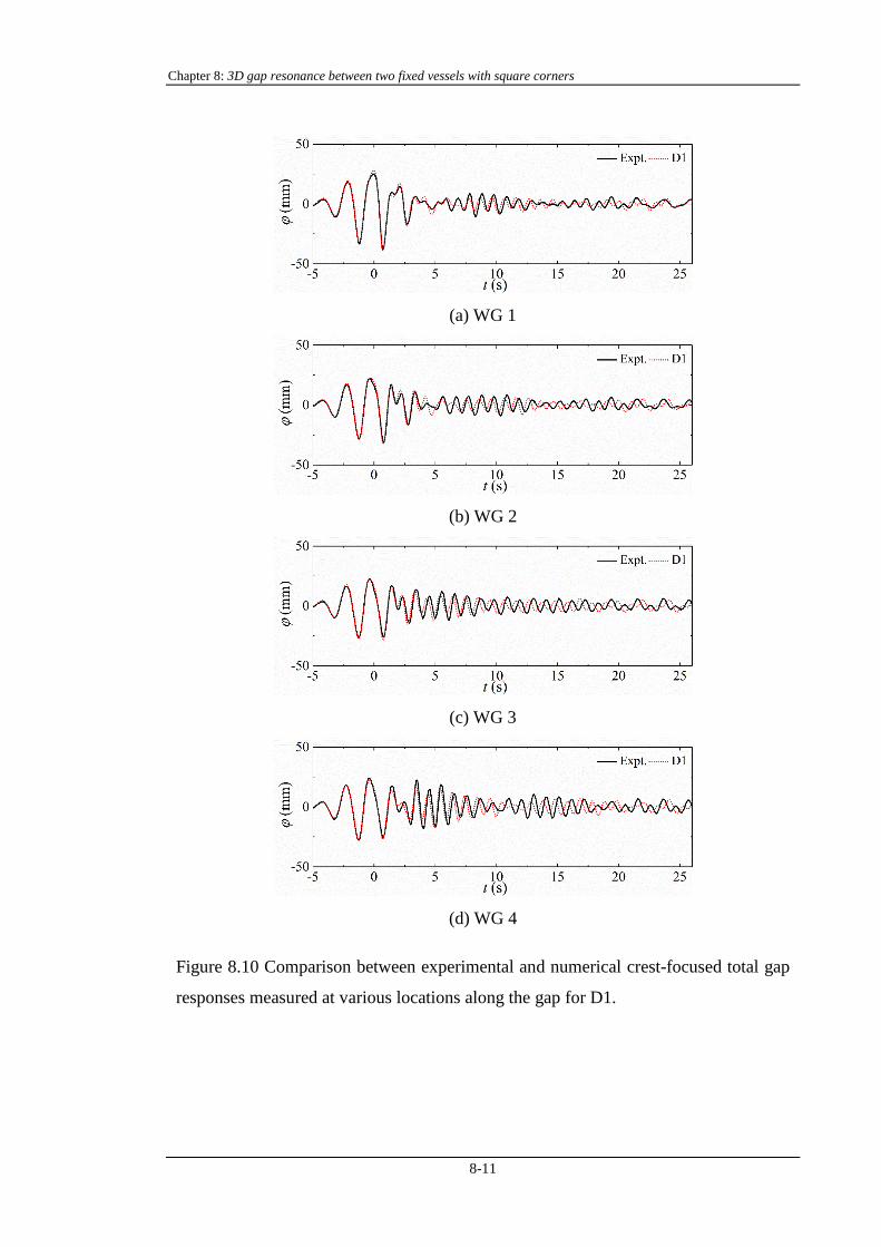
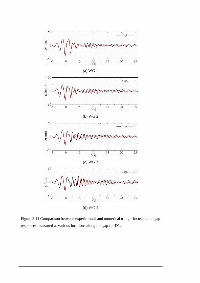
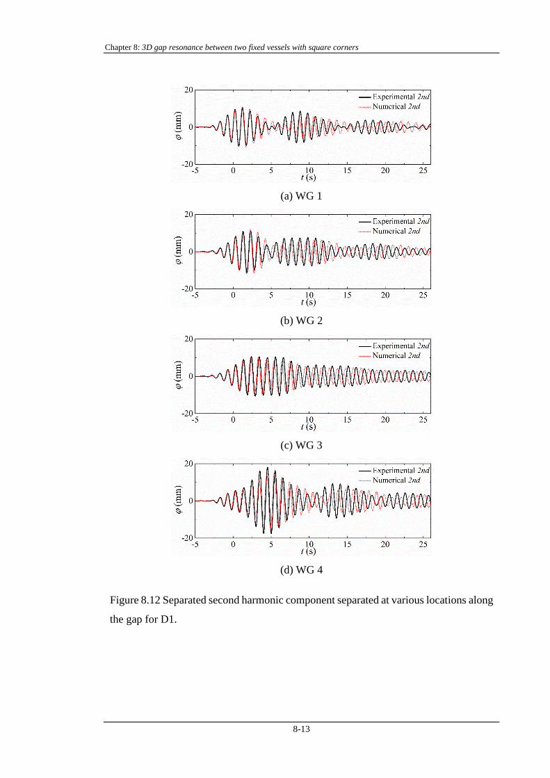
A mesh D1 with Δ𝑥2=2 mm was used for the simulations for Set D. The crest-focused
and trough-focused gap responses measured at WG 1-4 are shown in Figure 8.10 and
Figure 8.11. The second harmonic component is extracted using the phase inversion
harmonic extraction method and the results are shown in Figure 8.12. The same trend in
phase between the experimental and the numerical results are found in the time series.
Applying the method of Kumaresan and Tufts to the time series for the second harmonic
component, the resonant frequency and damping coefficient for each mode are obtained
as listed in Table 8.2. It is found the numerical results still over-predict the resonant
frequencies. In terms of damping coefficients, the numerical results give very good
agreement with the experiment for the first and third modes, but the fifth mode is
obviously underpredicted by the CFD model (though the amplitude of the fifth mode is
small and is of less importance). Two caveats of obtaining the damping coefficients are
discussed here. Firstly, the method of Kumaresan and Tufts assumes linear superposition
of modes. If the damping is quadratic in the velocity for the square corner case, this
Chapter 8: 3D gap resonance between two fixed vessels with square corners
8-11
(a) WG 1
(b) WG 2
(c) WG 3
(d) WG 4
Figure 8.10 Comparison between experimental and numerical crest-focused total gap
responses measured at various locations along the gap for D1.
(a) WG 1
(b) WG 2
(c) WG 3
(d) WG 4
Figure 8.11 Comparison between experimental and numerical trough-focused total gap
responses measured at various locations along the gap for D1.
Chapter 8: 3D gap resonance between two fixed vessels with square corners
8-13
(a) WG 1
(b) WG 2
(c) WG 3
(d) WG 4
Figure 8.12 Separated second harmonic component separated at various locations along
the gap for D1.
(a) (b)
Figure 8.13 Dependency of the resonant frequency for each mode on (a) gap width (b)
draft using Molin’s method.
analysis will not perform as well as in the round corner (linear) case. Therefore, the
method of Kumaresan and Tufts must be treated with some caution, though the trends in
frequencies and damping are consistent with the time series. Secondly, if the damping is
quadratic it means the drag force is proportional to the square of the amplitude of gap
oscillation, but it enters odd harmonics when expanded into harmonic components (see
Fitzgerald et al., 2014). This breaks the Stokes’ structure assumed to exist for the phase
inversion harmonic extraction method.
8.4 Discussion
From the numerical results for Set C and Set D, the resonant frequencies are always over
predicted by the numerical model. Given the good prediction of the resonant frequencies
(or phase) for the round corner setup, it is quite unexpected that the resonant frequencies
for the square corner setup are not well predicted by the CFD model. This means there
might be some flow features existing in the experiments which are not captured or
resolved in the CFD model. To investigate the differences in more detail, several possible
causes are considered below.
Chapter 8: 3D gap resonance between two fixed vessels with square corners
8-15
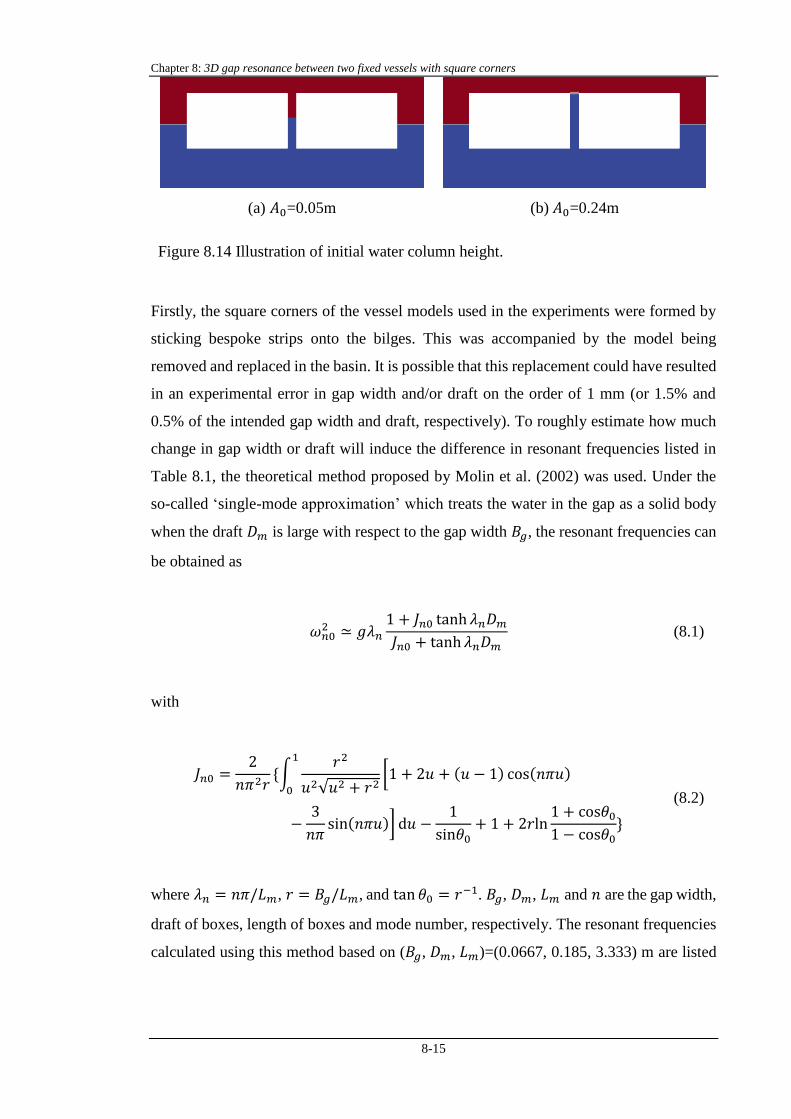
(a) 𝐴0=0.05m (b) 𝐴0=0.24m
Figure 8.14 Illustration of initial water column height.
Firstly, the square corners of the vessel models used in the experiments were formed by
sticking bespoke strips onto the bilges. This was accompanied by the model being
removed and replaced in the basin. It is possible that this replacement could have resulted
in an experimental error in gap width and/or draft on the order of 1 mm (or 1.5% and
0.5% of the intended gap width and draft, respectively). To roughly estimate how much
change in gap width or draft will induce the difference in resonant frequencies listed in
Table 8.1, the theoretical method proposed by Molin et al. (2002) was used. Under the
so-called ‘single-mode approximation’ which treats the water in the gap as a solid body
when the draft 𝐷𝑚 is large with respect to the gap width 𝐵𝑔, the resonant frequencies can
be obtained as
𝜔𝑛02 ≃ 𝑔𝜆𝑛
1 + 𝐽𝑛0 tanh 𝜆𝑛𝐷𝑚𝐽𝑛0 + tanh𝜆𝑛𝐷𝑚
(8.1)
with
𝐽𝑛0 =2
𝑛𝜋2𝑟{∫
𝑟2
𝑢2√𝑢2 + 𝑟2[1 + 2𝑢 + (𝑢 − 1) cos(𝑛𝜋𝑢)
1
0
−3
𝑛𝜋sin(𝑛𝜋𝑢)] d𝑢 −
1
sin𝜃0+ 1 + 2𝑟ln
1 + cos𝜃01 − cos𝜃0
}
(8.2)
where 𝜆𝑛 = 𝑛𝜋/𝐿𝑚, 𝑟 = 𝐵𝑔/𝐿𝑚, and tan 𝜃0 = 𝑟−1. 𝐵𝑔, 𝐷𝑚, 𝐿𝑚 and 𝑛 are the gap width,
draft of boxes, length of boxes and mode number, respectively. The resonant frequencies
calculated using this method based on (𝐵𝑔, 𝐷𝑚, 𝐿𝑚)=(0.0667, 0.185, 3.333) m are listed
(a) Coarse mesh (b) Fine mesh
Figure 8.15 Illustration of mesh near the gap entrance.
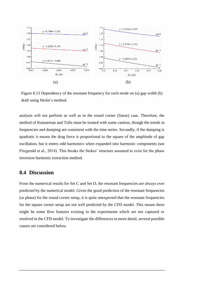
in Table 8.1. It is found that Molin’s method predicts the resonant frequency reasonably
well for the first mode, but over-predicts the resonant frequencies for the third mode and
the fifth mode. According to Eq. (8.1), the dependencies of the resonant frequency for
each mode on gap width (while fixing draft) and draft (while fixing gap width) are shown
in Figure 8.13(a) and (b) respectively, in which the curves can be fitted using a linear
function over the range of interest. It is found that a 1% change in gap width while fixing
draft will result in 0.14%, 0.08%, 0.04% change in the resonant frequencies for the first,
third and fifth modes respectively. In turn, a 1% change in draft while fixing gap width
will result in 0.32%, 0.28% and 0.19% change in the resonant frequencies for the first,
third and fifth modes respectively. This means that the resonant frequencies are more
sensitive to a change in draft than a change in gap width. Taking C2 as an example, the
resonant frequency for the first mode over predicts the experiment by 1.5%, meaning a
10.5% change in gap width or 4.7% change in draft would be required to cause such
frequency difference, which is very unlikely to occur in the experiment.
A second possible cause of the frequency over-prediction is under-resolution of the flow
around the entrance of the gap, with possible effects on the ‘added mass’ or volume of
water oscillating within the gap. To check the effect of the mesh under the boxes (whilst
minimising computational time) a series of 2D decay tests were carried out by releasing
a water column with predefined initial height in a gap formed by two fixed boxes. The
2D configuration was the same as the cross-section in the mid-ship plane for the 3D gap
resonance problem. Two initial water column heights were used as illustrated in Figure
8.14, i.e. 𝐴0=50 mm, which is approximately the level of the maximum gap response for
the 3D experimental results (referred to as ‘standard case’), and 𝐴0=240 mm, which is an
extreme case with an initial elevation set equal to the top of the boxes (referred to as
Chapter 8: 3D gap resonance between two fixed vessels with square corners
8-17
(a) 𝐴0=50 mm, ‘standard case’
(b) 𝐴0=240 mm, ‘extreme case’
Figure 8.16 Time series of free surface elevation in the gap with different meshes.
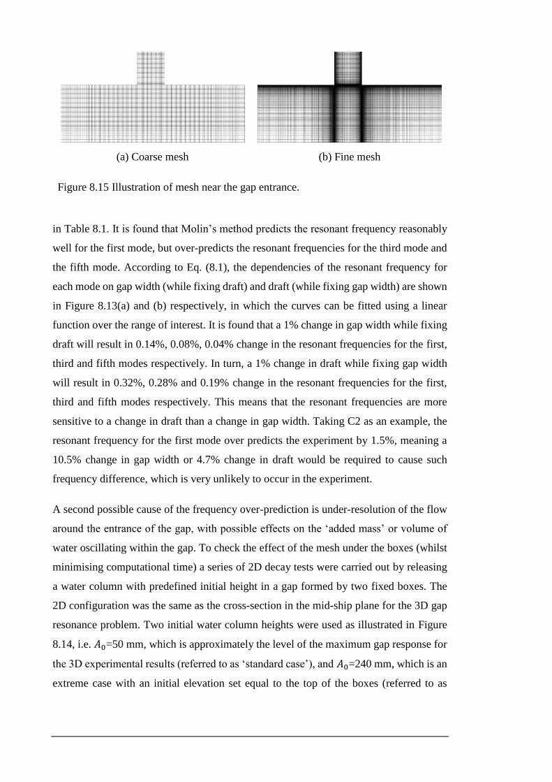
‘extreme case’). Two meshes were used for both cases as shown in Figure 8.15, i.e. a
coarse mesh with near-wall cell width Δ𝑥2=2 mm, and a fine mesh with near-wall cell
width Δ𝑥2=0.1 mm and refined mesh under the boxes. After release, the water column in
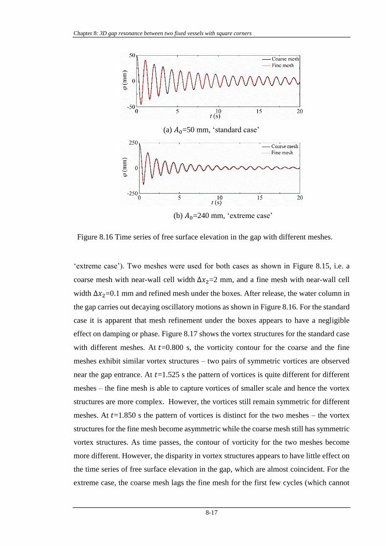
the gap carries out decaying oscillatory motions as shown in Figure 8.16. For the standard
case it is apparent that mesh refinement under the boxes appears to have a negligible
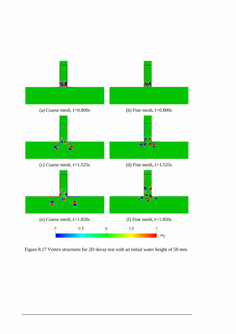
effect on damping or phase. Figure 8.17 shows the vortex structures for the standard case
with different meshes. At 𝑡=0.800 s, the vorticity contour for the coarse and the fine
meshes exhibit similar vortex structures – two pairs of symmetric vortices are observed
near the gap entrance. At 𝑡=1.525 s the pattern of vortices is quite different for different
meshes – the fine mesh is able to capture vortices of smaller scale and hence the vortex
structures are more complex. However, the vortices still remain symmetric for different
meshes. At 𝑡=1.850 s the pattern of vortices is distinct for the two meshes – the vortex
structures for the fine mesh become asymmetric while the coarse mesh still has symmetric
vortex structures. As time passes, the contour of vorticity for the two meshes become
more different. However, the disparity in vortex structures appears to have little effect on
the time series of free surface elevation in the gap, which are almost coincident. For the
extreme case, the coarse mesh lags the fine mesh for the first few cycles (which cannot
(a) Coarse mesh, 𝑡=0.800s (b) Fine mesh, 𝑡=0.800s
(c) Coarse mesh, 𝑡=1.525s (d) Fine mesh, 𝑡=1.525s
(e) Coarse mesh, 𝑡=1.850s (f) Fine mesh, 𝑡=1.850s
Figure 8.17 Vortex structures for 2D decay test with an initial water height of 50 mm.
𝜔𝑦
Chapter 8: 3D gap resonance between two fixed vessels with square corners
8-19
Figure 8.18 Comparison of time series of free surface elevation in the gap for initial
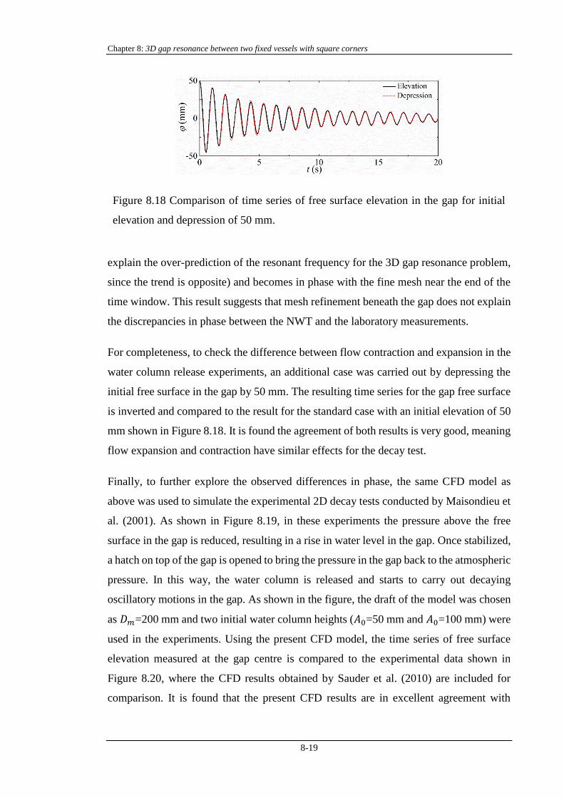
elevation and depression of 50 mm.
explain the over-prediction of the resonant frequency for the 3D gap resonance problem,
since the trend is opposite) and becomes in phase with the fine mesh near the end of the
time window. This result suggests that mesh refinement beneath the gap does not explain
the discrepancies in phase between the NWT and the laboratory measurements.
For completeness, to check the difference between flow contraction and expansion in the
water column release experiments, an additional case was carried out by depressing the
initial free surface in the gap by 50 mm. The resulting time series for the gap free surface
is inverted and compared to the result for the standard case with an initial elevation of 50
mm shown in Figure 8.18. It is found the agreement of both results is very good, meaning
flow expansion and contraction have similar effects for the decay test.
Finally, to further explore the observed differences in phase, the same CFD model as
above was used to simulate the experimental 2D decay tests conducted by Maisondieu et
al. (2001). As shown in Figure 8.19, in these experiments the pressure above the free
surface in the gap is reduced, resulting in a rise in water level in the gap. Once stabilized,
a hatch on top of the gap is opened to bring the pressure in the gap back to the atmospheric
pressure. In this way, the water column is released and starts to carry out decaying
oscillatory motions in the gap. As shown in the figure, the draft of the model was chosen
as 𝐷𝑚=200 mm and two initial water column heights (𝐴0=50 mm and 𝐴0=100 mm) were
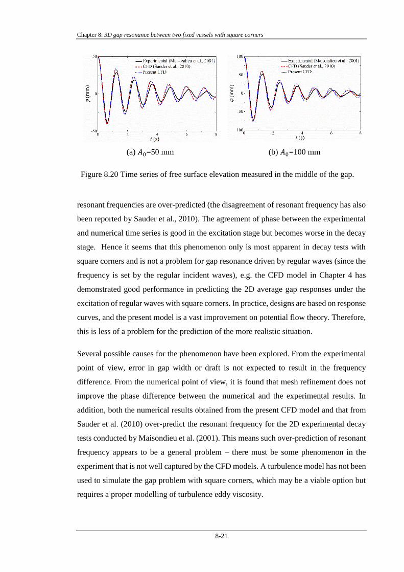
used in the experiments. Using the present CFD model, the time series of free surface
elevation measured at the gap centre is compared to the experimental data shown in
Figure 8.20, where the CFD results obtained by Sauder et al. (2010) are included for
comparison. It is found that the present CFD results are in excellent agreement with
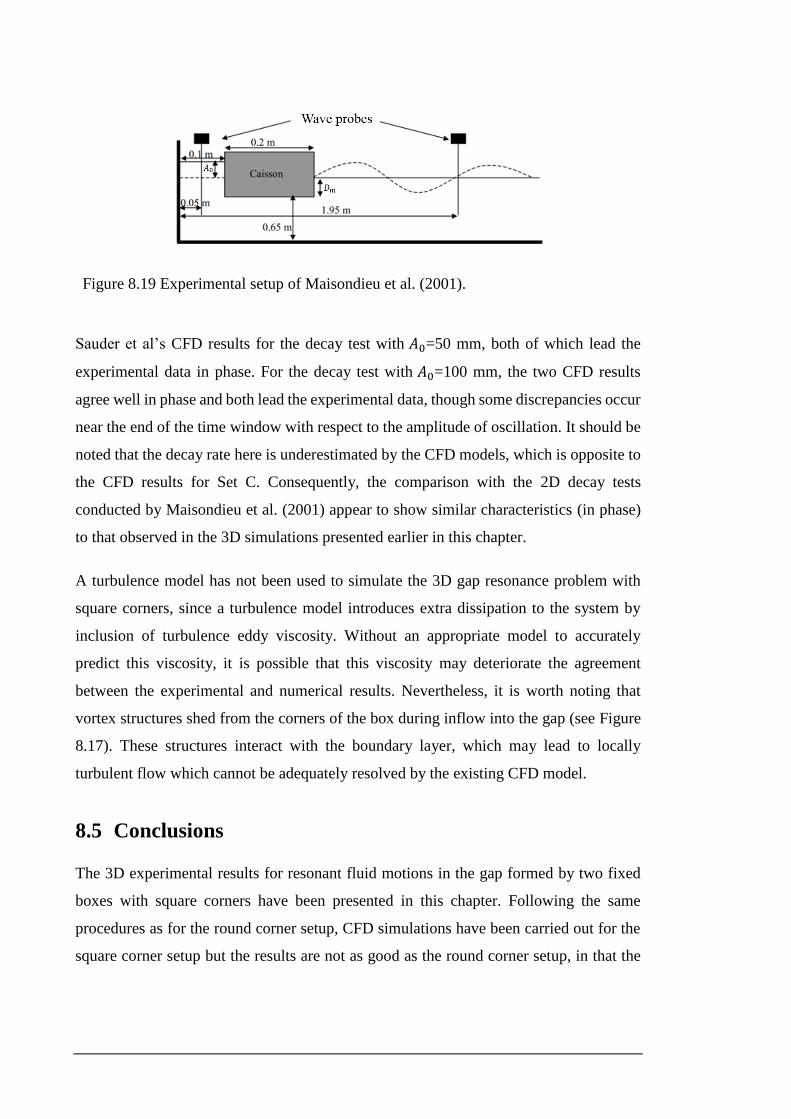
Figure 8.19 Experimental setup of Maisondieu et al. (2001).
Sauder et al’s CFD results for the decay test with 𝐴0=50 mm, both of which lead the
experimental data in phase. For the decay test with 𝐴0=100 mm, the two CFD results
agree well in phase and both lead the experimental data, though some discrepancies occur
near the end of the time window with respect to the amplitude of oscillation. It should be
noted that the decay rate here is underestimated by the CFD models, which is opposite to
the CFD results for Set C. Consequently, the comparison with the 2D decay tests
conducted by Maisondieu et al. (2001) appear to show similar characteristics (in phase)
to that observed in the 3D simulations presented earlier in this chapter.
A turbulence model has not been used to simulate the 3D gap resonance problem with
square corners, since a turbulence model introduces extra dissipation to the system by
inclusion of turbulence eddy viscosity. Without an appropriate model to accurately
predict this viscosity, it is possible that this viscosity may deteriorate the agreement
between the experimental and numerical results. Nevertheless, it is worth noting that
vortex structures shed from the corners of the box during inflow into the gap (see Figure
8.17). These structures interact with the boundary layer, which may lead to locally
turbulent flow which cannot be adequately resolved by the existing CFD model.
8.5 Conclusions
The 3D experimental results for resonant fluid motions in the gap formed by two fixed
boxes with square corners have been presented in this chapter. Following the same
procedures as for the round corner setup, CFD simulations have been carried out for the
square corner setup but the results are not as good as the round corner setup, in that the
Chapter 8: 3D gap resonance between two fixed vessels with square corners
8-21
(a) 𝐴0=50 mm (b) 𝐴0=100 mm
Figure 8.20 Time series of free surface elevation measured in the middle of the gap.
resonant frequencies are over-predicted (the disagreement of resonant frequency has also
been reported by Sauder et al., 2010). The agreement of phase between the experimental
and numerical time series is good in the excitation stage but becomes worse in the decay
stage. Hence it seems that this phenomenon only is most apparent in decay tests with
square corners and is not a problem for gap resonance driven by regular waves (since the
frequency is set by the regular incident waves), e.g. the CFD model in Chapter 4 has
demonstrated good performance in predicting the 2D average gap responses under the
excitation of regular waves with square corners. In practice, designs are based on response
curves, and the present model is a vast improvement on potential flow theory. Therefore,
this is less of a problem for the prediction of the more realistic situation.
Several possible causes for the phenomenon have been explored. From the experimental
point of view, error in gap width or draft is not expected to result in the frequency
difference. From the numerical point of view, it is found that mesh refinement does not
improve the phase difference between the numerical and the experimental results. In
addition, both the numerical results obtained from the present CFD model and that from
Sauder et al. (2010) over-predict the resonant frequency for the 2D experimental decay
tests conducted by Maisondieu et al. (2001). This means such over-prediction of resonant
frequency appears to be a general problem – there must be some phenomenon in the
experiment that is not well captured by the CFD models. A turbulence model has not been
used to simulate the gap problem with square corners, which may be a viable option but
requires a proper modelling of turbulence eddy viscosity.

Page intentionally left blank
Chapter 9: Conclusions
9-1
9 CONCLUSIONS
9.1 Introduction
This thesis is concerned with using CFD to estimate the resonant water motions in the
gap between two fixed boxes arranged in a parallel configuration at lab-scale, which is
representative of a side-by-side offloading scenario. By solving the Navier-Stokes
equations combined with the free surface captured by VOF method, both 2D and 3D
numerical simulations under the excitation of regular waves and transient focused wave
groups respectively, have been carried out to successfully reproduce the physical
experiments. Flow field information in high spatial and temporal resolution has been
utilized to explain the phenomena found in the experiments. Unlike most previous
numerical studies on this topic which are concerned with predicting the time-averaged
responses in the gap, the reproduction of the much more demanding time series of gap
responses included in this thesis has made the study very ambitious and challenging,
especially for a 3D configuration where multiple spatial modal structures are present and
the flow-structure interactions are more complex. The mesh size in the boundary layer
can be 𝑂(104) times smaller than the wavelength scale, which has led to significant
computational effort being required for the simulations as well as the post-processing. In
this chapter, the main conclusions of the work are summarised according to the aims set
out in Chapter 2 and possible future research is suggested.
9.2 Conclusions
9.2.1 Two-dimensional gap resonance between two fixed vessels
• Mesh convergence studies for 2D gap resonance under the excitation of regular
waves with round and sharp corners have been carried out. It is found that the
time-averaged gap responses for sharp corners are not affected significantly by
the near-wall cell width normal to the wall, which is consistent with the finding
by Kristiansen & Faltinsen (2012). On the contrary, the gap responses for round
corners are highly sensitive to the near-wall cell width normal to the wall. This
implies wall friction is more important for round corners than sharp corners. The
response curve of gap responses with square corners is in good agreement with
the experimental results obtained by Saitoh et al. (2006).
• With respect to the amplitude of resonant gap responses with different entrance
shapes, it has been shown that the round entrance results in the largest response,
the bilge keel the smallest and the square entrance an intermediate response. This
is consistent with the results for round and square corners found by Moradi et al.
(2015). Since the response is damped by entrance and exit energy losses of flow
in the gap, these rankings are analogous to fluid flowing from/to a reservoir
into/from a pipe with round, protruded and square entrance shape. By utilizing an
equivalent linearized viscous damping model (Tan et al., 2018), the damping
coefficients are found to be smallest for the round entrance shape while largest for
the bilge keel entrance shape, which explains the difference in resonant amplitude
between the gap responses for different entrance shapes. The resonant frequencies
for square and bilge keel entrance shapes are close to each other, while that for
the round entrance shape is larger. This is because there is little change in ‘added
mass’ when the entrance shape is altered from square corner to bilge keel, whereas
the trapped volume of fluid in the gap is reduced when the entrance shape is
modified from square corner to round corner.
• With increasing incident wave amplitude (or equivalently amplitude of gap
oscillation), the resonant wave elevation in the gap will increase while the peak
of response curves will decrease for all entrance shapes, which is related to the
increasing damping coefficients in the system. When the amplitude of gap
oscillation increases, the resonant frequency exhibits different trends for different
entrance shapes. This can be explained by the nonlinear damping effect and the
Duffing-like behaviour with a hardening spring associated with the nonlinear free
surface conditions. The former will result in a decrease in resonance frequency
while the latter will cause the opposite trend.
• Instead of running a series of long-time regular wave tests, simulations of a few
cycles of decay following release of an initial water column in the gap can be used
to predict the resonant frequency of gap responses. The results of this method have
Chapter 9: Conclusions
9-3
shown very good agreement with the resonant frequencies identified from the
response curves for different entrance shapes, amplitudes of gap oscillation and
water depths.
• Scaling effects are investigated approximately by varying fluid viscosity in the
numerical simulations. It is found the scaling effects (or effects of varying
viscosity) lead to greater changes in response amplitude for round corners than
square corners. Though the present model may not be able to resolve all fluid
structures in the large-scale (low viscosity) simulations, this does suggest one
should be careful when interpreting results in the laboratory to predict results in
the field, especially for vessels with round corners.
9.2.2 Development of a numerical wave tank to simulate 3D gap
resonance between two fixed vessels with round corners
• A 3D NWT for gap resonance with round corners has been successfully
established by systematically optimizing the mesh topology and extent, together
with appropriate boundary conditions for the purpose of replicating the physical
experiments conducted by Zhao et al. (2017). The meshing strategy is based on
physical insights to resolve both the wave and boundary layer scales. Within the
computational domain, the boundary layer thickness will be the smallest length
scale and require the finest mesh. To improve efficiency the key is to have the
highest possible aspect ratio for this fine mesh, so that upstream of the boxes the
propagation of the incident waves can be simulated reliably without overly fine
vertical resolution.
• Various iterative methods have been employed to recreate the experimental
incident transient wave groups. The linear iterative method shows the best result,
by adjusting the amplitude and phase information based on the difference between
the recorded linear wave signal in the NWT and the desired linear wave signal.
9.2.3 Linear excitation of 3D gap resonance between two fixed vessels
with round corners
• Without any parametric tuning, the 3D numerical time series of gap responses,
resonant amplitudes and frequencies, and mode shapes have shown very good
agreement with the experimental data obtained by Zhao et al. (2017). It is
demonstrated that the near-wall cell width normal to the wall must be sufficiently
small to resolve the boundary layer to accurately reproduce the experimental
results. As the near-wall mesh becomes finer, the time series of gap responses
become closer to the experimental results.
• Interrogation of flow field information finds that nearly all the viscous dissipation
is confined to a thin layer surrounding the boxes, meaning the contribution from
flow separation is negligible and wall friction is the main source of damping.
Using the validated numerical data, the near-wall boundary layer can be well
predicted by solving the Stokes equation using the time-varying pressure
measured at a position near the wall in the gap but still outside the boundary layer.
The near-wall boundary layer has been decomposed into modal components
which gives excellent agreement with the theoretical Stokes boundary layer
solution. Collectively, these pieces of numerical evidence strongly support the
postulation by Zhao et al. (2017) that the viscous damping beyond the radiation
damping affecting the decaying gap oscillations in their experiments was linear.
• The viscous dissipation in the boundary layer has been computed, separated into
modes and added to the modal radiation damping contribution to produce modal
global damping coefficients in reasonable agreement with those estimated from
the decay of the free surface in the simulation. Both sets of damping coefficients
show modestly good agreement with the experimental values.
• The vertical and spanwise velocities can be regarded as a superposition of various
mode shapes as well. The mode shapes for the vertical velocity follow the free
surface elevation, while the mode shapes for the spanwise velocity are inverse.
The vertical velocity is found to be dominant in the gap, meaning the
simplification of a 3D gap resonance model to its 2D counterpart is somewhat
possible.
9.2.4 Frequency-doubling excitation of 3D gap resonance between two
fixed vessels with round corners
• The experimental results of frequency doubling excitation including first, second
and third harmonics of free surface elevation have been successfully reproduced
in the NWT. The numerical fourth harmonic component is self-consistent in a way
Chapter 9: Conclusions
9-5
that the scaled squared envelopes of the second harmonic component match the
time series of the fourth harmonic component remarkably well. This represents a
highly successful application of CFD to a problem with linear viscous dissipation
but nonlinear free surface effects, both of which must be resolved to achieve
satisfactory results. This is expected to have important application to swell
excitation of gap resonance.
• Mode shapes for the free surface are successfully captured up to the fifteenth and
agree well with the experimental data. The first to the seventh mode shapes are
identified from the second harmonic component, while the ninth to the fifteenth
mode shapes are identified from the third harmonic component.
• The harmonic structures for the velocity in the gap and forces on the boxes have
been extracted successfully using a phase-inversion harmonic extraction method.
Significant shielding from the up-wave box is observed in the excitation stage
such that the wave loading on the up-wave box is much larger than that on the
down-wave box.
9.2.5 3D gap resonance between two fixed vessels with square corners
• 3D gap resonance with square corners excited by transient wave groups has been
simulated in the NWT and the results are compared to the available experimental
data obtained by Zhao et al. (2017). It is found that the CFD model generally
overpredicts the resonant frequencies and damping coefficients, with the
discrepancy between numerical results and experiment substantially greater than
for the round corner cases. The overprediction of resonant frequencies will result
in a phase lead accumulating over time. Several possible causes for the
overprediction of resonant frequencies have been investigated. It is found that the
error in gap width or draft in the experiment is very unlikely to cause such
frequency difference and refining the mesh in the CFD model does not improve
the results.
• 2D decay tests of a water column with predefined initial heights in a gap with
square corners have been simulated using the present CFD model. The results are
compared to the experimental data by Maisondieu et al. (2001) and also the
numerical results by Sauder et al. (2010). It is found the present CFD results agree
well with those obtained from Sauder et al. (2010), both of which lead the
experimental data over time. This means the phenomenon is not a coincidence and
may generally exist for decay tests in a gap with square corners. The results imply
that there are flow behaviours which exist in the laboratory but are not captured
by the CFD models used for comparison.
9.3 Future research
9.3.1 Gap resonance at larger scales
This thesis primarily contributes to understanding resonant fluid behaviours in gaps at
lab-scale. Ultimately the gap resonance problem has industrial relevance at a substantially
larger scale and conclusions drawn from lab-scale in this thesis may need to be revisited
at larger scales. For gaps with round corners at lab-scale, it is expected the viscous
damping is dominated by laminar boundary layer damping, though flow separation may
sometimes occur. As the scale is increased, the boundary layer will inevitably become
turbulent and flow separation will contribute more of the damping. For square (sharp)
corners flow separation will occur in the lab as well as in the field.
In this thesis, the scaling effect is touched on via varying the fluid velocity in 2D
numerical simulations. The numerical results suggest that the scaling effect is more
important for round corners than square corners since the gap responses for round corners
increase dramatically when the scale is increased towards a prototype scale. However, it
should be noted that the same mesh (converged at lab-scale) has been used to study the
2D gap resonance problem at different scales (or with different viscosity). This is not a
problem for scales smaller than the lab-scale, but the mesh is not expected to resolve all
aspects of the flows at larger scales. Therefore, further study should be carried out to
consider gap resonance at larger scales with a more appropriate numerical setup
(turbulence models may be needed) to verify these results.
It is favourable to investigate scaling effects on 2D gap resonance in the first place,
considering it is much less computationally costly than its 3D counterpart. For 3D gap
resonance at larger scales, it would be tempting to start simulations with square corners
first, if the gap responses at larger scales are not affected much by the mesh in the gap (it
is reasonable to have such expectation given the 2D time-averaged gap responses with
square corners excited by regular waves have smaller scaling effects and are almost
independent of the mesh in the gap at lab-scale). This may allow us to use a relatively
coarse mesh to simulate the problem, which is at least 20 times faster than a fine mesh,
Chapter 9: Conclusions
9-7
based on the experience gained here. It can be much more difficult to simulate 3D gap
resonance with round corners at larger scales since the mesh in the gap should be
adequately fine to resolve turbulent boundary layers and flow separation at a point
dependent on the Reynolds number. Ultimately field data collected from a full-scale
facility would be invaluable and serve to shed some light on these fundamental issues
associated with scaling.
9.3.2 3D Gap resonance with different headings
Only beam sea conditions are considered in this thesis. In real sea states the offloading
vessels are exposed to external waves incident from different headings. For headings
other than beam sea condition both odd (symmetric) and even (antisymmetric) mode
shapes are present along the gap. To enable CFD simulations in a NWT for different
headings, several points are important. Firstly, oblique sea conditions break down the
symmetry in geometry (as in beam sea conditions), preventing the use of symmetry
boundary conditions to save computational cost. Secondly, considering wave reflection
caused by incident waves interacting with the vessels and radiation from the first mode
(of most concern) can have larger influence on the responses in the gap for head and
oblique sea conditions, wave absorption at the side-walls are required. Finally,
unstructured mesh may be needed for oblique sea conditions and the performance of
resolving, e.g. wave as well as boundary layer scales, should be examined.
9.3.3 Gap resonance with moving vessels
This thesis is concerned with the gap resonance problem with two fixed vessels. For
industrial applications the amplitude of the resonance during operations may be important
in its own right, or due to its coupling with vessel motion. For a moving body there is an
addition nonlinearity caused by the change of gap width in time, which is not investigated
in this study. Therefore, it is desirable to extend the scope of the work to consider gap
resonance with moving vessels. To this end, dynamic mesh should be used. To realise
motions of rigid bodies within the framework of OpenFOAM, many researchers choose
to extend the two-phase solver ‘interDyMFoam’ with dynamic mesh handling coupled
with a motion solver. Higuera et al. (2015) and Dao et al. (2018) modelled physical
movements of piston wave paddles and flap paddles, respectively, to realise wave
generation in a NWT. Schmitt and Elsaesser (2015) simulated the rotational motion of a
flap-type oscillating wave surge converter in waves by making extensions to the
‘interDyMFoam’ libraries in terms of equations of motion and mesh motion algorithm.
The numerical model reproduces the experimental data within the bounds of experimental
accuracy. Devolder et al. (2017) simulated free decay tests and regular wave tests for
heaving wave energy converters, and the numerical results show reasonable agreement
with the experimental data.
Despite the above applications of modelling rigid body motions using OpenFoam, it
should be admitted that dynamic mesh is more difficult to handle than static mesh and
sometimes numerical stability is a problem. For the gap resonance problem, simulations
with moving vessels are more challenging than for a single body case in that the mesh
deformation can be problematic due to the narrow gap width and should be treated with
caution. Hence, development of a reliable solver as well as mesh algorithm is required
for the successful simulation of gap resonance with moving vessels. To break down the
complexity, a step-by-step procedure should be carried out, by considering the motion of
one vessel first and releasing the degrees of freedom one by one.
References
1
REFERENCES
Adcock, T.A., Taylor, P.H., 2016. Non-linear evolution of uni-directional focussed wave-
groups on a deep water: A comparison of models. Applied Ocean Research 59, 147-
152.
Almeida, R., 2012. New Maritime Additions to the Iron Ore Trade, Vale’s Ore Fabrica
and Mitsui’s Tom Price. from https://gcaptain.com/maritime-additions-iron-trade/.
Bartzis, J.G., 2004. Thematic area 5: Best practice advice for environmental flows. The
QNET-CFD Network Newsletter 2, 34-39.
Berberović, E., van Hinsberg, N.P., Jakirlić, S., Roisman, I.V., Tropea, C., 2009. Drop
impact onto a liquid layer of finite thickness: Dynamics of the cavity evolution.
Physical Review E 79 (3), 036306.
Buchner, B., Van Dijk, A., De Wilde, J., 2001. Numerical multiple-body simulations of
side-by-side mooring to an FPSO, The Eleventh International Offshore and Polar
Engineering Conference. International Society of Offshore and Polar Engineers.
Burel, F., Taccani, R., Zuliani, N., 2013. Improving sustainability of maritime transport
through utilization of Liquefied Natural Gas (LNG) for propulsion. Energy 57, 412-
420.
Center, E.s.G.O.G., 2013. Global LNG - Will new demand and new supply mean new
pricing? Ernst & Young.
Chaplin, J.R., 1996. On frequency-focusing unidirectional waves. International Journal
of Offshore and Polar Engineering 6 (02).
Chen, X.-B., 2005. Hydrodynamic analysis for offshore LNG terminals, Proceedings of
the 2nd International Workshop on Applied Offshore Hydrodynamics, Rio de Janeiro.
Chua, K.H., de Mello, P., Malta, E., Vieira, D., Watai, R., Ruggeri, F., Taylor, R.E.,
Nishimoto, K., Choo, Y.S., 2018. Irregular Seas Model Experiments on Side-by-Side
Barges, The 28th International Ocean and Polar Engineering Conference. International
Society of Offshore and Polar Engineers.
Clauss, G.F., Dudek, M., Testa, D., 2013. Gap effects at side-by-side LNG-transfer
operations, ASME 2013 32nd International Conference on Ocean, Offshore and Arctic
Engineering. American Society of Mechanical Engineers, pp. V001T001A042-
V001T001A042.
Dao, M.H., Chew, L.W., Zhang, Y., 2018. Modelling physical wave tank with flap paddle
and porous beach in OpenFOAM. Ocean Engineering 154, 204-215.
Devolder, B., Rauwoens, P., Troch, P., 2017. Numerical simulation of an array of heaving
floating point absorber wave energy converters using openfoam, 7th International
Conference on Computational Methods in Marine Engineering (MARINE), pp. 777-
788.
Dodge, E., 2014. How Dangerous is LNG? from
https://breakingenergy.com/2014/12/22/how-dangerous-is-lng/.
Eatock Taylor, R., 2007. On modelling the diffraction of water waves. Ship Technology
Research 54 (2), 54-80.
Faltinsen, O., Newman, J., Vinje, T., 1995. Nonlinear wave loads on a slender vertical
cylinder. Journal of Fluid Mechanics 289, 179-198.
Faltinsen, O., Timokha, A., 2015. On damping of two-dimensional piston-mode sloshing
in a rectangular moonpool under forced heave motions. Journal of Fluid Mechanics
772.
Faltinsen, O.M., Rognebakke, O.F., Timokha, A.N., 2007. Two-dimensional resonant
piston-like sloshing in a moonpool. Journal of Fluid Mechanics 575, 359-397.
Feng, X., Bai, W., 2015. Wave resonances in a narrow gap between two barges using
fully nonlinear numerical simulation. Applied Ocean Research 50, 119-129.
Feng, X., Bai, W., Chen, X., Qian, L., Ma, Z., 2017. Numerical investigation of viscous
effects on the gap resonance between side-by-side barges. Ocean Engineering 145, 44-
58.
Fernández, H., Sriram, V., Schimmels, S., Oumeraci, H., 2014. Extreme wave generation
using self correcting method—Revisited. Coastal Engineering 93, 15-31.
Fitzgerald, C., Taylor, P., Eatock Taylor, R., Grice, J., Zang, J., 2014. Phase manipulation
and the harmonic components of ringing forces on a surface-piercing column, Proc. R.
Soc. A. The Royal Society, p. 20130847.
References
3
Fredriksen, A.G., Kristiansen, T., Faltinsen, O.M., 2015. Wave-induced response of a
floating two-dimensional body with a moonpool. Philosophical Transactions of the
Royal Society of London A: Mathematical, Physical and Engineering Sciences 373
(2033), 20140109.
Giacosa, A., Mauries, B., Lagarrigue, V., 2016. Joining Forces to Unlock LNG Tandem
Offloading Using 20? LNG Floating Hoses: An Example of Industrial Collaboration,
Offshore Technology Conference. Offshore Technology Conference.
Gibson, R., Swan, C., 2007. The evolution of large ocean waves: the role of local and
rapid spectral changes, Proceedings of the Royal Society of London A: Mathematical,
Physical and Engineering Sciences. The Royal Society, pp. 21-48.
Greenshields, C.J., 2015. OpenFOAM user guide. OpenFOAM Foundation Ltd, version
3 (1).
Groizeleau, V., 2016. Ideol: foundations for floating wind turbines. from
https://www.meretmarine.com/fr/content/ideol-foundations-floating-wind-turbines.
Hann, M., Greaves, D., Raby, A., 2014. A new set of focused wave linear combinations
to extract non-linear wave harmonics, Intl Workshop on Water Waves and Floating
Bodies.
Håvardstun, T., 2013. Moonpool. from
https://www.youtube.com/watch?v=KofiI6XyCX0.
Higuera, P., Lara, J.L., Losada, I.J., 2013. Realistic wave generation and active wave
absorption for Navier–Stokes models: Application to OpenFOAM®. Coastal
Engineering 71, 102-118.
Higuera, P., Losada, I.J., Lara, J.L., 2015. Three-dimensional numerical wave generation
with moving boundaries. Coastal Engineering 101, 35-47.
Hirt, C.W., Nichols, B.D., 1981. Volume of fluid (VOF) method for the dynamics of free
boundaries. Journal of computational physics 39 (1), 201-225.
Hong, S.Y., Kim, J.H., Kim, H.J., Choi, Y.R., 2002. Experimental study on behavior of
tandem and side-by-side moored vessels, Proceedings of The 12th International
Offshore and Polar Engineering Conference, Kitakyushu, Japan.
Huang, C.-J., Zhang, E.-C., Lee, J.-F., 1998. Numerical simulation of nonlinear viscous
wavefields generated by piston-type wavemaker. Journal of Engineering Mechanics
124 (10), 1110-1120.
Huijsmans, R., Pinkster, J., De Wilde, J., 2001. Diffraction and radiation of waves around
side-by-side moored vessels, The Eleventh International Offshore and Polar
Engineering Conference. International Society of Offshore and Polar Engineers.
Hunt, A., Taylor, P., Borthwick, A., Stansby, P., Feng, T., 2002. Focused waves onto a
plane beach. Trans. R. Soc. Lond. A 354, 649-676.
IGU, 2017. World LNG report. IGU World LNG Report—2017 Edition.
Jacobsen, N.G., 2017. waves2Foam Manual.
Jacobsen, N.G., Fuhrman, D.R., Fredsøe, J., 2012. A wave generation toolbox for the
open‐ source CFD library: OpenFoam®. International Journal for Numerical
Methods in Fluids 70 (9), 1073-1088.
Jasak, H., 1996. Error Analysis and Estimation for the finite volume method with
applications to fluid flows. Thesis submitted for the degree of doctor. Department of
Mechanical Engineering, Imperial College of Science, 1996.
Jensen, B.L., Sumer, B.M., Fredsøe, J., 1989. Turbulent oscillatory boundary layers at
high Reynolds numbers. Journal of Fluid Mechanics 206, 265-297.
Jiang, S.-C., Bai, W., Cong, P.-W., Yan, B., 2019. Numerical investigation of wave forces
on two side-by-side non-identical boxes in close proximity under wave actions. Marine
Structures 63, 16-44.
Jiang, S.-C., Bai, W., Tang, G.-Q., 2018. Numerical simulation of wave resonance in the
narrow gap between two non-identical boxes. Ocean Engineering 156, 38-60.
Jin, Y., Chai, S., Duffy, J., Chin, C., Bose, N., 2018. URANS predictions on the
hydrodynamic interaction of a conceptual FLNG-LNG offloading system in regular
waves. Ocean Engineering 153, 363-386.
John, F., 1950. On the motion of floating bodies II. Simple harmonic motions.
Communications on pure and applied mathematics 3 (1), 45-101.
Kristiansen, T., Faltinsen, O.M., 2008. Application of a vortex tracking method to the
piston-like behaviour in a semi-entrained vertical gap. Applied Ocean Research 30 (1),
1-16.
Kristiansen, T., Faltinsen, O.M., 2009. Studies on resonant water motion between a ship
and a fixed terminal in shallow water. Journal of Offshore Mechanics and Arctic
Engineering-Transactions of the Asme 131 (2), 021102.
References
5
Kristiansen, T., Faltinsen, O.M., 2012. Gap resonance analyzed by a new domain-
decomposition method combining potential and viscous flow DRAFT. Applied Ocean
Research 34, 198-208.
Kristiansen, T., Sauder, T., Firoozkoohi, R., 2013. Validation of a hybrid code combining
potential and viscous flow with application to 3D moonpool, Proceedings of the
ASME 2013 32nd International Conference on Ocean, Offshore and Arctic
Engineering (OMAE2013).
Kumar, S., Kwon, H.-T., Choi, K.-H., Lim, W., Cho, J.H., Tak, K., Moon, I., 2011. LNG:
An eco-friendly cryogenic fuel for sustainable development. Applied Energy 88 (12),
4264-4273.
Kumaresan, R., Tufts, D., 1982. Estimating the parameters of exponentially damped
sinusoids and pole-zero modeling in noise. IEEE Transactions on Acoustics, Speech,
and Signal Processing 30 (6), 833-840.
Kuznetsov, N., McIver, P., 1997. On uniqueness and trapped modes in the water-wave
problem for a surface-piercing axisymmetric body. The Quarterly Journal of
Mechanics and Applied Mathematics 50 (4), 565-580.
Lamb, H., 1932. Hydrodynamics. Hydrodynamics, by Horace Lamb and Foreword by
Russ Caflisch, pp. 764. ISBN 0521458684. Cambridge, UK: Cambridge University
Press, November 1993., 764.
Lee, C.-H., Newman, J.N., 2004. Computation of wave effects using the panel method,
in: Chakrabarti, S. (Ed.), Numerical models in fluid-structure interaction,
Southhampton.
Lin, P., Liu, P.L.-F., 1999. Internal wave-maker for Navier-Stokes equations models.
Journal of waterway, port, coastal, and ocean engineering 125 (4), 207-215.
Loose, A., Caswell, C., Bentley, M., LeBoeuf, R., D'Souza, R., 2014. Early FLNG
projects deal with technical and execution challenges. from https://www.offshore-
mag.com/articles/print/volume-74/issue-5/engineering-construction-
installation/early-flng-projects-deal-with-technical-and-execution-challenges.html.
Lu, L., Teng, B., Cheng, L., Li, Y., 2008. Numerical simulation of hydrodynamic
resonance in a narrow gap between twin bodies subject to water waves, The Eighteenth
International Offshore and Polar Engineering Conference. International Society of
Offshore and Polar Engineers.

Ma, Y., Dong, G., Liu, S., Zang, J., Li, J., Sun, Y., 2009. Laboratory study of
unidirectional focusing waves in intermediate depth water. Journal of Engineering
Mechanics 136 (1), 78-90.
Maddock, I., Harby, A., Kemp, P., Wood, P.J., 2013. Ecohydraulics: an integrated
approach. John Wiley & Sons.
Maisondieu, C., Molin, B., Kimmoun, O., Gentaz, L., 2001. Simulation
bidimensionnelles des écoulements dans une baie de forage. Etude des modes de
résonance et des amortissements, 8ème Journées de l'Hydrodynamique.
McIver, M., 1996. An example of non-uniqueness in the two-dimensional linear water
wave problem. Journal of Fluid Mechanics 315 (-1), 257.
McIver, M., Porter, R., 2002. Trapping of waves by a submerged elliptical torus. Journal
of Fluid Mechanics 456, 277-293.
McIver, P., 2005. Complex resonances in the water-wave problem for a floating structure.
Journal of Fluid Mechanics 536, 423-443.
McIver, P., McIver, M., 1997. Trapped modes in an axisymmetric water-wave problem.
The Quarterly Journal of Mechanics and Applied Mathematics 50 (2), 165-178.
McIver, P., McIver, M., 2006. Trapped modes in the water-wave problem for a freely
floating structure. Journal of Fluid Mechanics 558, 53-67.
McIver, P., McIver, M., 2007. Motion trapping structures in the three-dimensional water-
wave problem. Journal of Engineering Mathematics 58 (1-4), 67-75.
McIver, P., Newman, J., 2003. Trapping structures in the three-dimensional water-wave
problem. Journal of Fluid Mechanics 484, 283-301.
Mei, C.C., Stiassnie, M., Yue, D.K.-P., 1989. Theory and Applications of Ocean Surface
Waves: Part 1: Linear Aspects Part 2: Nonlinear Aspects. World Scientific.
Meylan, M.H., Eatock Taylor, R., 2009. Time-dependent water-wave scattering by arrays
of cylinders and the approximation of near trapping. Journal of Fluid Mechanics 631,
103-125.
Molin, B., 2001. On the piston and sloshing modes in moonpools. Journal of Fluid
Mechanics 430, 27-50.
Molin, B., 2017. On natural modes in moonpools with recesses. Applied Ocean Research
67, 1-8.
References
7
Molin, B., Remy, F., Camhi, A., Ledoux, A., 2009. Experimental and numerical study of
the gap resonances in-between two rectangular barges, 13th Congress of Intl. Maritime
Assoc. of Mediterranean IMAM 2009.
Molin, B., Remy, F., Kimmoun, O., Stassen, Y., 2002. Experimental study of the wave
propagation and decay in a channel through a rigid ice-sheet. Applied Ocean Research
24 (5), 247-260.
Molin, B., Zhang, X., Huang, H., Remy, F., 2018. On natural modes in moonpools and
gaps in finite depth. Journal of Fluid Mechanics 840, 530-554.
Moradi, N., Zhou, T., Cheng, L., 2015. Effect of inlet configuration on wave resonance
in the narrow gap of two fixed bodies in close proximity. Ocean Engineering 103, 88-
102.
Moradi, N., Zhou, T., Cheng, L., 2016. Two-dimensional numerical study on the effect
of water depth on resonance behaviour of the fluid trapped between two side-by-side
bodies. Applied Ocean Research 58, 218-231.
Newby, M.A., Pauw, W., 2010. SS-Safe Transfer of Liquefied Gas in the Offshore
Environment, Offshore Technology Conference. Offshore Technology Conference.
Newman, J., 1999. Radiation and diffraction analysis of the McIver toroid. Journal of
Engineering Mathematics 35 (1), 135-147.
Newman, J., Sclavounos, P., 1988. The computation of wave loads on large offshore
structures, Proc. of Int. Conf. on Behaviour of Offshore Structures (BOSS’88), pp.
605-622.
Patankar, S., 1980. Numerical heat transfer and fluid flow. CRC press.
Paulsen, B.T., Bredmose, H., Bingham, H.B., Jacobsen, N.G., 2014. Forcing of a bottom-
mounted circular cylinder by steep regular water waves at finite depth. Journal of Fluid
Mechanics 755, 1-34.
Pauw, W.H., Huijsmans, R.H., Voogt, A., 2007. Advances in the hydrodynamics of side-
by-side moored vessels, ASME 2007 26th International Conference on Offshore
Mechanics and Arctic Engineering. American Society of Mechanical Engineers, pp.
597-603.
Perić, M., Swan, C., 2015. An experimental study of the wave excitation in the gap
between two closely spaced bodies, with implications for LNG offloading. Applied
Ocean Research 51, 320-330.
Poldervaart, L., Oomen, H., Ellis, J., 2006. Offshore LNG transfer: a worldwide review
of offloading availability, Offshore Technology Conference. Offshore Technology
Conference.
Saitoh, T., Miao, G., Ishida, H., 2006. Theoretical analysis on appearance condition of
fluid resonance in a narrow gap between two modules of very large floating structure,
Proceedings of the Third Asia-Pacific Workshop on Marine Hydrodynamics,
Shanghai, China, pp. 170-175.
Sauder, T., Kristiansen, T., Ostman, A., 2010. Validation of a numerical method for the
study of piston-like oscillations between a ship and a terminal, The Twentieth
International Offshore and Polar Engineering Conference. International Society of
Offshore and Polar Engineers.
Schäffer, H.A., 1996. Second-order wavemaker theory for irregular waves. Ocean
Engineering 23 (1), 47-88.
Schäffer, H.A., Stolborg, T., Hyllested, P., 1994. Simultaneous generation and active
absorption of waves in flumes. Proc., waves-physical and numerical modelling. Dept.
of Civ. Engrg., University of British Columbia, Vancouver, 90-99.
Schmitt, P., Elsaesser, B., 2015. On the use of OpenFOAM to model oscillating wave
surge converters. Ocean Engineering 108, 98-104.
Schmittner, C., Kosleck, S., Hennig, J., 2009. A phase-amplitude iteration scheme for the
optimization of deterministic wave sequences, ASME 2009 28th International
Conference on Ocean, Offshore and Arctic Engineering. American Society of
Mechanical Engineers, pp. 653-660.
SHELL, 2017. Outlook 2017. SHELL.
Shipway, B., Evans, D., 2002. Wave trapping by axisymmetric concentric cylinders,
ASME 2002 21st International Conference on Offshore Mechanics and Arctic
Engineering. American Society of Mechanical Engineers, pp. 705-712.
Simon, M., Ursell, F., 1984. Uniqueness in linearized two-dimensional water-wave
problems. Journal of Fluid Mechanics 148, 137-154.
Stagonas, D., Buldakov, E., Simons, R., 2014. Focusing unidirectional wave groups on
finite water depth with and without currents. Coastal Engineering Proceedings 1 (34),
31.
References
9
Statoil, 2017. Spectaculair hoogstandje Dockwise. from
https://www.schuttevaer.nl/nieuws/offshore/nid27848-spectaculair-hoogstandje-
dockwise.html.
Sumer, B.M., Fredsøe, J., 2006. Hydrodynamics Around Cylindrical Structures. World
Scientific.
Sun, L., Eatock Taylor, R., Taylor, P.H., 2010. First-and second-order analysis of
resonant waves between adjacent barges. Journal of Fluids and Structures 26 (6), 954-
978.
Tan, L., Lu, L., Tang, G., Cheng, L., Chen, X., 2017. An energy dissipation model for
wave resonance problems in narrow gaps formed by floating structures, Proc. 32nd
Int. Workshop Water Waves Float. Bodies.
Tan, L., Lu, L., Tang, G., Cheng, L., Chen, X., 2018. A viscous damping model for wave-
induced response of fluid in narrow gaps or moonpools. Submitted to Journal of Fluid
Mechanics.
Teigen, P., Niedzwecki, J., 2006. A Computational Study of Wave Effects Related to
Side-by-Side LNG Offoading, The Sixteenth International Offshore and Polar
Engineering Conference. International Society of Offshore and Polar Engineers.
Tromans, P.S., Anaturk, A.R., Hagemeijer, P., 1991. A new model for the kinematics of
large ocean waves-application as a design wave, The First International Offshore and
Polar Engineering Conference. International Society of Offshore and Polar Engineers.
Vinje, T., 1991. An approach to the non-linear solution of the oscillating water column.
Applied Ocean Research 13 (1), 18-36.
Voogt, A.J., Brugts, H., 2010. SS: LPG & LNG Offshore Operations: Numerical
simulations to optimize offshore offloading operations, Offshore Technology
Conference. Offshore Technology Conference.
Voser, P., 2012. Shell: Global Natural Gas Demand to Increase 60% by 2030. from
https://www.offshoreenergytoday.com/shell-global-natural-gas-demand-to-increase-
60-by-2030/.
Vyzikas, T., Stagonas, D., Buldakov, E., Greaves, D., 2015. Efficient numerical
modelling of focused wave groups for freak wave generation, The Twenty-fifth
International Offshore and Polar Engineering Conference. International Society of
Offshore and Polar Engineers.
Walker, D., Taylor, P., Taylor, R.E., 2004. The shape of large surface waves on the open
sea and the Draupner New Year wave. Applied Ocean Research 26 (3-4), 73-83.
Whitham, G., 1963. The Navier-Stokes equations of motion. Laminar boundary layers,
114-162.
Wilhelmsen, 2017. Global LNG Outlook to 2030 from a Shipping Perspective, Spotlight
on Australia, Korea and Japan.
Wolgamot, H., Taylor, P., Eatock Taylor, R., van den Bremer, T., Raby, A., Whittaker,
C., 2016. Experimental observation of a near-motion-trapped mode: free motion in
heave with negligible radiation. Journal of Fluid Mechanics 786.
Zhao, W., Milne, I., Efthymiou, M., Wolgamot, H., Draper, S., Taylor, P., Taylor, R.E.,
2018a. Current practice and research directions in hydrodynamics for FLNG-side-by-
side offloading. Ocean Engineering 158, 99-110.
Zhao, W., Taylor, P.H., Wolgamot, H.A., Eatock Taylor, R., 2018b. Linear viscous
damping in random wave excited gap resonance at laboratory scale—NewWave
analysis and reciprocity. Journal of Fluids and Structures 80, 59-76.
Zhao, W., Wolgamot, H., Taylor, P., Eatock Taylor, R., 2017. Gap resonance and higher
harmonics driven by focused transient wave groups. Journal of Fluid Mechanics 812,
905-939.


![Correlated magnetic noise across Virgo and spatially ... · global resonance may occur [14]. Natural Schumann resonance excitation is mostly caused by lightning discharges. Lightning](https://img.pdfslide.net/doc/110x75/5f0b7b177e708231d430baad/correlated-magnetic-noise-across-virgo-and-spatially-global-resonance-may-occur.jpg)