Physics 171/271 - Chapter 7R - David Kleinfeld - Fall 2005

7 Networks of Phase Coupled Neuronal Oscilla-

tors

We consider small networks or simple networks in which cells are coupled onlyweakly, in the sense that then can effect each others timing but do not necessarilyturn each other on or off.

7.1 Basic formalism

Equation of motion for a general dynamical system

d ~X

dt= F ( ~X;µ) (7.1)

where the ~X is a vector that contains all the dynamical variables and the µ areparameters. At steady state

d ~X0

dt= F ( ~X0;µ) (7.2)

where a closed orbit satisfies

~X0(t+ T ) = ~X0(t) (7.3)

FIGURE - chapt-12-kuromoto-1-2-3.eps

We associate a value of ψ with each point along ~X(t). Thus the multidimensionaltrajectory is reduced to a single variable.

It is useful to extend the definition of ψ off of the limit cycle, or contour, C, toall points within a tube around C so that ψ is defined for all ~X in the tube. Thiswill allow us to study perturbations to the original limit cycle.

Look on a surface, denoted G, normal to and in the neighborhood of C. Let Pbe a point on G and Q be the point on C, the limit cycle, that passes through thesame surface. We posit that as the trajectories evolve, the point P will approach theclosed orbit defined by C. There will be a phase difference between P and Q. Thisis equivalent to an initial phase difference among the points. The main idea is thatthe physical perturbation can be transformed into a phase shift along the originallimit cycle, C, if the perturbed point collapses to or forever parallels the originallimit cycle.

There are a set of points in the tube that will lead to the same phase shift. Thesedefine a surface of constant phase shifts, that is denoted I(ψ). For all points ~X onI(ψ) we have

1

dψ( ~X)

dt= ω (7.4)

for the unperturbed system. But, by the chain rule,

dψ

dt=

∑

i

∂ψ

∂Xi

∂Xi

∂t(7.5)

= ~∇ ~X ψ · d~X

dt

= ~∇ ~X ψ · ~F ( ~X)

Let’s perturb the motion by

~F ( ~X) → ~F ( ~X) + ǫ ~P ( ~X, ~X ′) (7.6)

where ǫ is small in the sense that the shape of the original trajectory in unchangedas ǫ → 0 and ~X ′ contains all the variables that define the perturbation, e.g, thetrajectory of a neighboring oscillator and the interaction between the two oscillatingsystems. Then

dψ

dt= ~∇ ~X ψ ·

[

F ( ~X) + ǫ ~P ( ~X, ~X ′)]

(7.7)

= ω + ǫ~∇ ~X ψ · ~P ( ~X, ~X ′)

So far everything is exact, that is, all calculations are done with respect to theperturbed orbit. The difficulty is that the orbits are not necessarily closed. But ifwe can make ǫ small enough so that | ~X(t)− ~X0(t)| → 0 as t→ ∞, the perturbationwill lead to a closed path. This results in periodic orbits, so that the independentvariable can now be taken as the phase, ψ, rather than time, t, where the two arerelated by

ψ = 2πt

Tmodulo(2π) (7.8)

Using

~X(t) → ~X0(ψ) (7.9)

we have

dψ

dt= ω + ǫ~∇ ~X0(ψ) ψ · ~P

[

~X0(ψ), ~X ′0(ψ

′)]

(7.10)

≡ ω + ǫ~Z(ψ) · ~P (ψ, ψ′)

The term ~Z(ψ) depends only on the limit cycle of the oscillator and defines thesensitivity of the phase to perturbation. It clearly varies along the limit cycle and is

2

sometimes called a ”phase-dependent sensitivity”. It may be calculated directly byevaluating the trajectory of points inside a tube around the original limit cycle, ormore expeditiously using a trick due to Bowtell, in which the perturbed system is

rewritten in the form d ~Xdt

= A(t) ~X, with A(t) = A(t+ T ), which can be shown tohave only one periodic solution. A cute way to find the periodic solution is to solve

the adjoint problem, d~Ydt

= AT (t)~Y , for which all of the solutions decay except for

the periodic one. From this one backs out ~Z(ψ).

The cool thing in that the oscillator is seen to rotate freely (ω term) with phase-shifts and frequency shifts that are determined solely by the perturbations. The term~P (ψ, ψ′), which can be calculated from the perturbation, allows these perturbationsto be interactions with neighbors.

Let’s look at the nature of the perturbation term. The idea is that this is small,so that the shift in frequency on one cycle is small. We consider

ψ = δψ + ωt (7.11)

Then the relative motion is given by

dδψ

dt= ǫ~Z(ψ) · ~P (ψ, ψ′) (7.12)

= ǫ~Z(δψ + ωt) · ~P (δψ + ωt, δψ′ + ωt)

This can be further simplified. To the extent that the change in ψ is small overone cycle, i.e., dδψ

dt<< ω, we can average the perturbation over a full cycle. We

write

dδψ

dt= Γ(δψ, δψ′) (7.13)

where

Γ(δψ, δψ′) =ǫ

2π

∫ π

−πdθ ~Z(δψ + θ) · ~P (δψ + θ, δψ′ + θ) (7.14)

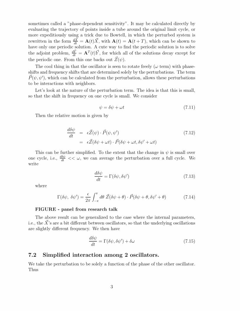
FIGURE - panel from research talk

The above result can be generalized to the case where the internal parameters,i.e., the ~X’s are a bit different between oscillators, so that the underlying oscillationsare slightly different frequency. We then have

dδψ

dt= Γ(δψ, δψ′) + δω (7.15)

7.2 Simplified interaction among 2 oscillators.

We take the perturbation to be solely a function of the phase of the other oscillator.Thus

3

Γ(δψ, δψ′) =ǫ

2π

∫ π

−πdθ ~Z(δψ + θ) · ~P (δψ′ + θ) (7.16)

But this is just a correlation integral that is proportion to the differences inphase, i.e.,

Γ(δψ′ − δψ) =ǫ

2π

∫ π

−πdθ ~Z (θ − (δψ′ − δψ)) · ~P (θ) (7.17)

So that a system of two oscillators obeys

dδψ

dt= Γ(δψ′ − δψ) (7.18)

dψ′

dt= Γ(δψ − δψ′)

We subtract the two equations of motion for the phase to get

d(δψ − δψ′)

dt= [Γ(δψ′ − δψ) − Γ(δψ − δψ′)] (7.19)

≡ Γ̃(δψ′ − δψ)

≡ −Γ̃(δψ − δψ′)

FIGURES - 5 panels from research talk

The term Γ̃(δψ − δψ′) is an odd function with period T , with zeros at

x0 ≡ δψ − δψ′ = nT

2n = 1, 2, 3, ... (7.20)

and possibly other places. By way of analysis,

• The zeros correspond to phase locking.

• The stability depends on the sign of dΓ̃(x)dx

∣

∣

∣

x0

• dΓ̃dx

∣

∣

∣

x0

< 0 implies stability with even n; attractive - phases converge.

• dΓ̃dx

∣

∣

∣

x0

> 0 implies stability with odd n; repulsive - phases diverge.

7.3 Examples

7.3.1 Two oscillators with delayed coupling.

An interesting example due to Ermentrout is to consider two oscillators that interactby a synapse with a noninstantaneous rise time. Before we choose a realistic cellmodel, let’s try some analytical methods and choose a form of ~Z(δψ) that hasvariable sensitivity along the limit cycle. The simplest choice is Z(t) = sinωt, or

4

Z(δψ) = sin(δψ) (7.21)

The interaction is given by an ”α” function, i.e., P (t) = gτtτe−t/τ with φ =

ωt modulo(2π), i.e.,

P (δψ′) =g

τ

δψ′

ωτe−δψ

′/ωτ (7.22)

The convolutions for Γ̃ can be done explicitly to yield

(Γ̃(δψ − δψ′) = g(8π2)(ωτ)2 − 1

[1 + (ωτ)2]2sin(δψ − δψ′) (7.23)

This says that, for excitatory connections (g > 0), the synchronized state, i.e.,δψ′ = δψ, is stable only for τ < 1

ω. In contrast, for τ > 1

ωthe antiphastic state with

δψ′ − δψ = ±π is stable. The opposite condition holds for inhibitory connections(g < 0).

FIGURE - 2 panels from research talk

Interestingly, synchronous, all inhibitory networks are observed experimentally!

7.3.2 Two identical Hodgkin Huxley oscillators.

How well does the above analysis hold with more realistic cells.

FIGURE - chapt-12-if-syn-phase-calc.eps

Recall the Hodgkin Huxley equations for a point neuron, where ~X = (V, h,m, n)T ,i.e.,

∂V (t)

∂t=

−rm2πaτ

(

gNam3h(V − VNa) + gKn

4(V − VK) + gleak(V − Vl) + Isyn)

dh(V, t)

dt=

h∞(V ) − h(V, t)

τh(V )(7.24)

dm(V, t)

dt=

m∞(V ) −m(V, t)

τm(V )

dn(V, t)

dt=

n∞(V ) − n(V, t)

τn(V )

Hansel and later van Vreeswijk considered two Hodgkin Huxley cells with asynaptic current given by

Isyn = −Gsyn [V (t) − Vsyn]spikes∑

i

f(t− ti) (7.25)

5

where he used an ”alpha” function for f(t). The form of ~Z(ψ + t) is foundfrom directly evaluating perturbations to the limit cycle, which is found from theHodgkin-Huxley equations with Isyn = 0. The perturbation is given by

P (ψ + t, ψ′ + t) = −Gsyn [V (ψ + ωt) − Vsyn]spikes∑

i

f(ψ′ + ωt− ωti) (7.26)

The systematics as a function of α for fixed ω were explored by van Vreeswijk

FIGURE - chapt-12-hh-phase-model.eps

The phase as a function of Iext, really ω, for fixed α were explored by Hansel.He also examined where in the cycle the neuron is most sensitive to perturbations.

7.3.3 Two oscillators with different intrinsic frequency.

We take

Γ(δψ − δψ′) ≡ −Γ0 sin(δψ − δψ′) (7.27)

Then

dδψ

dt= Γ0 sin(δψ′ − δψ) + δω (7.28)

dδψ′

dt= Γ0 sin(δψ − δψ′) + δω′

The system will phase lock, for which dδψdt

= dδψ′

dt, so long as the interaction

strength can satisfy

Γ̃ = Γ0 sin(δψ′ − δψ) − Γ0 sin(δψ − δψ′) (7.29)

= −2Γ0 sin(δψ − δψ′) = δω − δω′ (7.30)

or

2Γ0

|δω′ − δω| > 1 (7.31)

The phase shift is just

δψ − δψ′ = sin−1

(

δω′ − δω

2Γ0

)

(7.32)

and the frequency under phase lock is

ωobserved = ω +δω + δω′

2(7.33)

The above are the two quantities are the ones measured in the lab!

6

FIGURE - panel from research talk

Outside of the phase locked region, the system undergoes quasiperiodic motionwith a time varying phase shift given by

δψ − δψ′ = 2 tan−1

√

(δω − δω′)2 − 4Γ20 tan

(√

(δω−δω′)2−4Γ2

0t

2

)

+ 2Γ0

δω − δω′

(7.34)

7.3.4 Chain of oscillators with δω ∝ ∆x: The example of Limax.

dδψx

dt= δωx +

∑

x 6=x′Γ(δψx − δψx′) (7.35)

with

δωx ∝ x+ constant (7.36)

When the system locks, there is a single frequency, but a gradient of phase shiftswith ∆ψx

dxgiven by a monotonic function of x, like ∆ψx

dx∝ constant, i.e., the phase

shift appears as a traveling wave. The data from Limax shows traveling wavesand a gradient of intrinsic frequencies. The article by Ermentrout and Kleinfeldsummarizes this and other data.

FIGURES - 4 panels from research talk

7.3.5 Two oscillators with propagation delays.

We again take

Γ(δψ − δψ′) ≡ −Γ0 sin(δψ − δψ′) (7.37)

Then

dδψ

dt= Γ0 sin(δψ′(t− τD) − δψ(t)) + δω0 (7.38)

dδψ′

dt= Γ0 sin(δψ(t− τD) − δψ′(t)) + δω0

where the frequencies δω0 are assumed to be equal. We assume a solution of theform

δω = δω0 − Γ0 cosα sin δωτD (7.39)

This is satisfied for

α =

{

0 if cosωτD ≥ 0π if cosωτD < 0

7

Thus we observe both frequency shifts and potential phase shifts. The syn-chronous stare is stable only for 0 < τD < π

2δω. The details of this relation will

change if the symmetry of the waveform changes, but the gist is correct.

8

0 1000 2000 3000 4000Time (ms)

0

20

40

60

Freq

uenc

y (H

z)

20

10

0

0 2 4-2-4Time (ms)

Cro

ss-c

orre

latio

n 0-2.5

10-12.5

17.5-20

0 1000 2000 3000 4000Time (ms)

0

10

20

-10

-20

Running cross-correlogram

Tim

e (m

s)

NEOCORTEX

Electrical synapses can promote close spike synchrony