7 Numerical implementation techniques of finite element

7 Numerical implementation techniques of

finite element methods

283

Contents

1. Modelling principles and boundary value problems in engineering sciences

2. Basics of numerical integration and differentiation

3. Basic 1D finite difference and collocation methods

– bars/rods, heat diffusion, seepage, electrostatics

4. Finite difference methods for two-variable problems

– heat diffusion

5. Energy methods and basic 1D finite element methods

– bars/rods, beams, heat diffusion, seepage, electrostatics

6. Basic 2D and 3D finite element methods

– heat diffusion, seepage

7. Numerical implementation techniques for finite element methods

8. Finite element methods for Euler−Bernoulli beams

9. Finite element methods for 2D and 3D elasticity

10. Algorithmic design in architectural engineering

CIV-E1060

Engineering Computation and Simulation

CIV-E1060 / 2020 / Jarkko Niiranen

284

Contents

1. Element point of view and assembly

2. Reference elements and coordinate transformations

Learning outcome

A. Recognizing the main differences between the global and local frames in FEM

B. Ability to assemble global FEM stiffness matrices from local contributes

C. Ability to derive and apply the basic reference element calculus of FEM

References

Text book 1: Sections 6.4−5, 7.1

Text book 2: Sections 1.12−15, 2.5−6,

3.1−10, A3.I

7 Numerical implementation techniques of

finite element methods


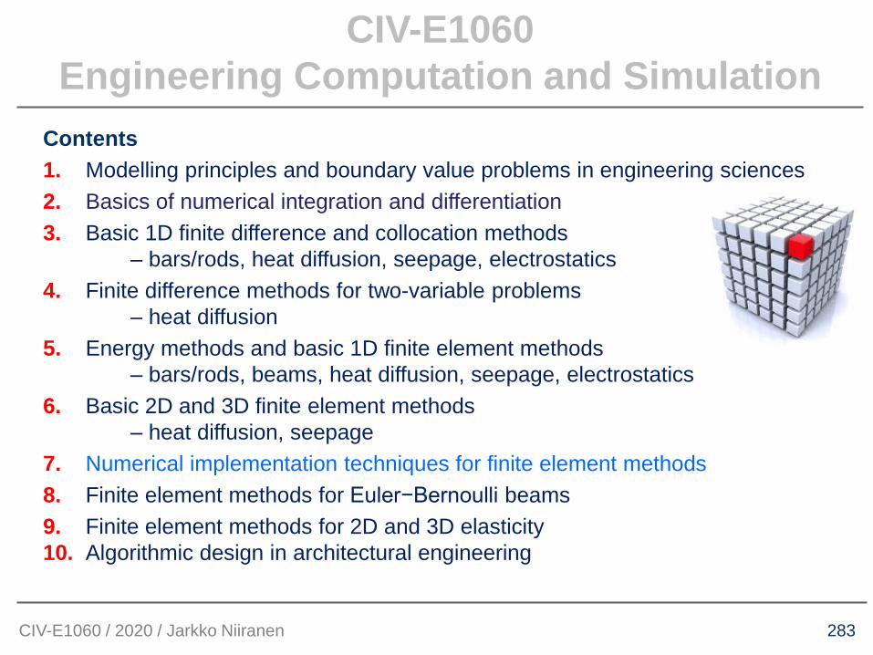
7.0 Programming finite element methods

285

What can you learn from the web pictures found by

using the keywords ”finite element implementation”?


287

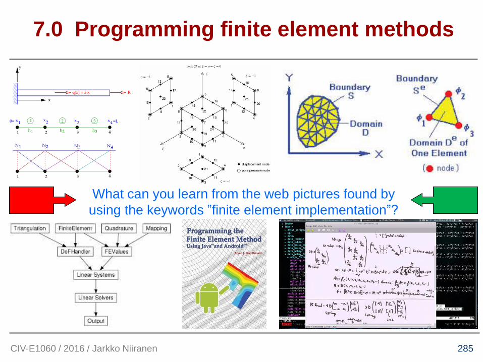
So far, all the finite element procedures have been considered from a nodal point of

view, or a basis function point of view – a global point of view: each basis function is

written in global coordinates and supported by more than one element.

Hence, both the (unknown) finite element solution

and its (unknown) global degrees of freedom (DOF) , as well as the final

equation system, are given in terms of the global basis functions (in terms of x):

j

n

j jnnh dxdxdxdxxu )()()()()(01100 =

=+++=

ijji x =)(

)( ihi xud =

i 1+i

ix 1+ix Lxn =00 =x

01

n

,fdK =

1+ie

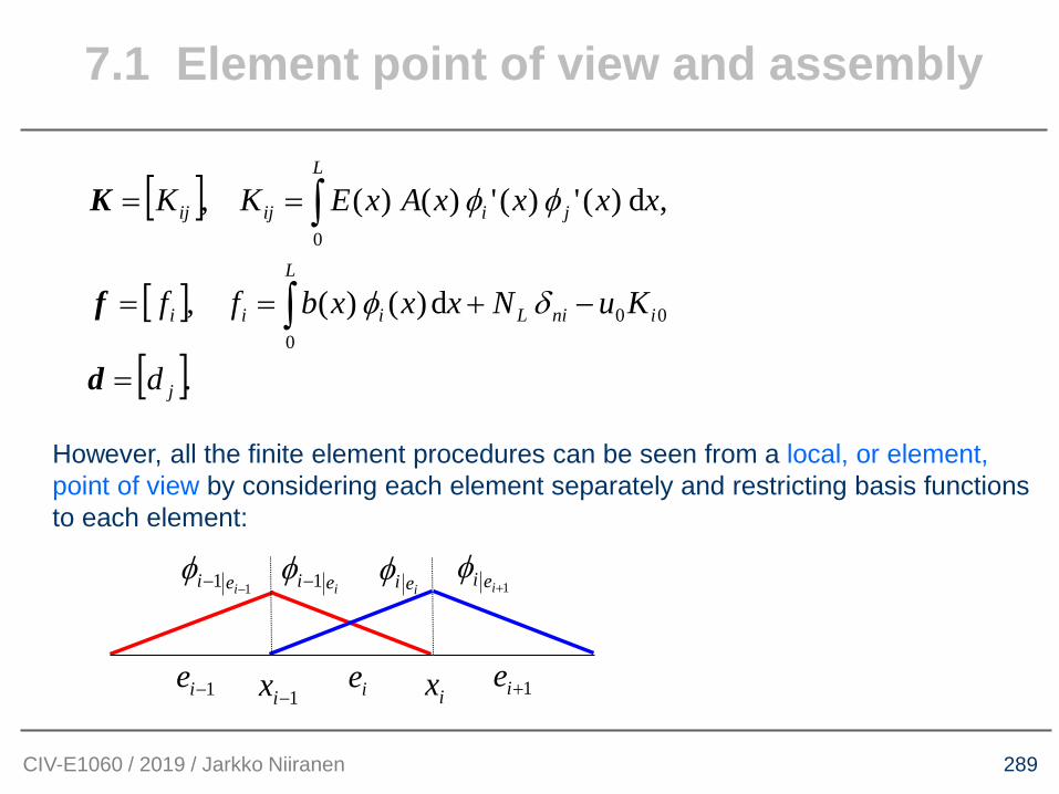
7.1 Element point of view and assembly


289

However, all the finite element procedures can be seen from a local, or element,

point of view by considering each element separately and restricting basis functions

to each element:

ie

iei 1−iei

1−ix ix1−ie 1+ie

11

−−

iei 1+iei

.

d)()(,

,d)(')(')()(,

00

0

0

j

iniL

L

iii

L

jiijij

d

KuNxxxbff

xxxxAxEKK

=

−+==

==

d

f

K



291

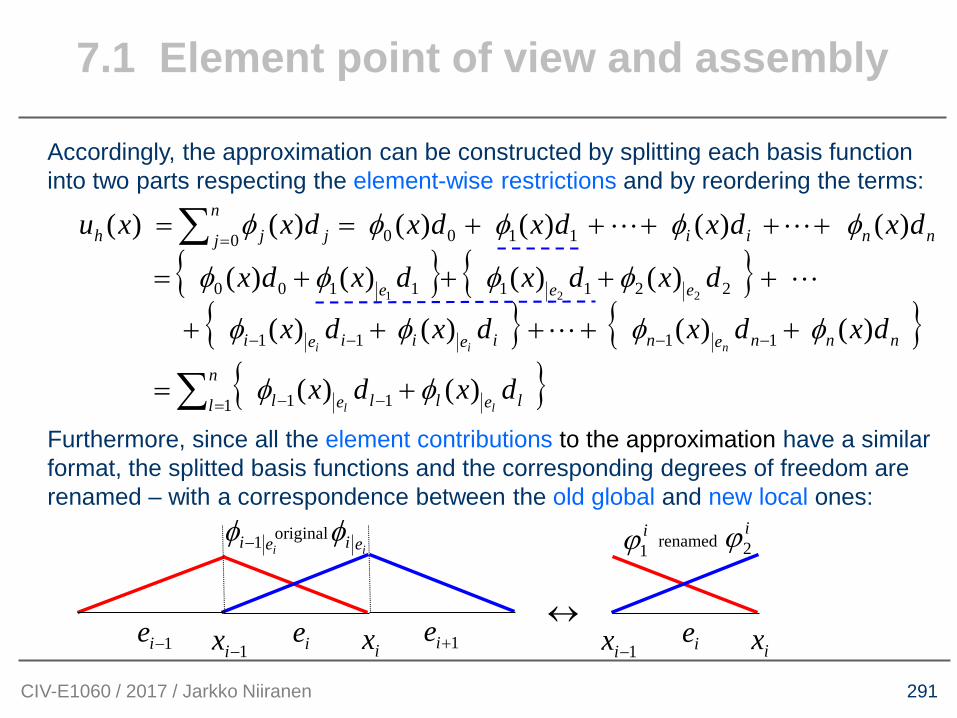
Accordingly, the approximation can be constructed by splitting each basis function

into two parts respecting the element-wise restrictions and by reordering the terms:

Furthermore, since all the element contributions to the approximation have a similar

format, the splitted basis functions and the corresponding degrees of freedom are

renamed – with a correspondence between the old global and new local ones:

ie

i

1i

2

1−ix ix

renamed

ie

iei 1−iei


original

= −−

−−−−

=

+=

+++++

++++=

+++++==

n

l lellel

nnnenieiiei

eee

nniij

n

j jh

dxdx

dxdxdxdx

dxdxdxdx

dxdxdxdxdxxu

ll

nii

1 11

1111

22111100

11000

)()(

)()()()(

)()()()(

)()()()()()(

221



292

Now, the approximation can be expressed as a sum of element contributions with

local basis functions and local degrees of freedom (properly related to global ones)

In each element, the approximation is hence of the form

llll

eh dxdxxul

2211 )()()( +=

le

l

1l

2

l

l

d

x

1

1−

l

l

d

x

2

renamed

=

= −−

+=

+=

n

l

llll

n

l lellelh

dxdx

dxdxxull

1 2211

1 11

)()(:

)()()(



293

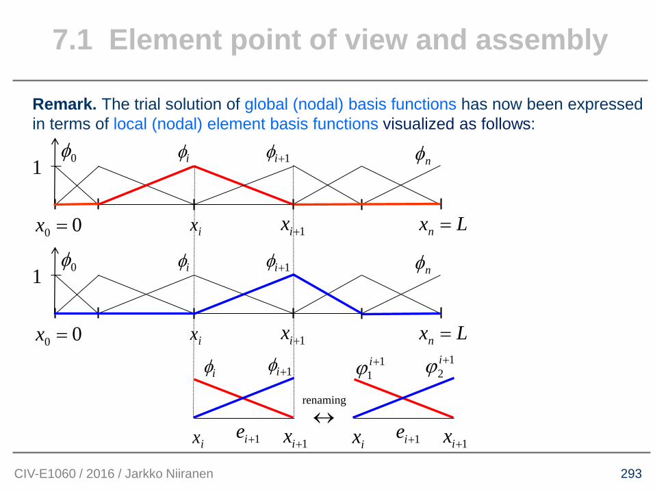
Remark. The trial solution of global (nodal) basis functions has now been expressed

in terms of local (nodal) element basis functions visualized as follows:

i 1+i

ix 1+ix Lxn =00 =x

01

n

i 1+i

ix 1+ix Lxn =00 =x

01

n

1+ie

i 1+i

ix 1+ix 1+ie

1

1

+i1

2

+i

ix 1+ix

renaming



298

Local (form of) stiffness matrix and force vector. A corresponding element-wise

splitting will be accomplished for the fairly local integrals of the stiffness matrix and

force vector entries by expressing them as sums of local integrals over elements.

For the 1D model problem, the discrete energy balance was earlier written in the

following form (weak form with inserted trial and test functions – note constants ci)

First, let us consider the right hand side of the equality, the load integral:

niNxbdxEA

ixbLNxdEA

xbLNxdEAc

xcbcLNxcdEA

niL

L

i

n

j j

L

ij

L

iiL

L

ij

n

j j

n

i

L

iiL

L

ij

n

j ji

L

i

n

i ii

n

i iL

L

i

n

i ij

n

j j

,,0dd''

d)(d''

0}d)(d''{

d)(d''

00 0

00 0

0 00 0

0

00

0

00

=+=

+=

=−−

+=

=

=

= =

====



302

( )

niL

ii

niLe

i

e

i

niL

n

l e

ii

niL

L

ii

Nff

Nxbxb

Nxb

Nxbf

ii

l

++=

++=

++=

+=

+

+

=

+

+

1

12

1

12

1

1

12

0

:

dd

d

d

1

( ) ( )

( ) ( ) ,d''

d''

d')'(d''

0 1

1

12

1

1

1

122

0

0

1

12

1

1

1

122

0 00 00

= =

+++

=

+++

===

++=

++=

=

=

n

j

n

l e

iijjjj

n

j

L

iijjjj

n

j

L

ijj

n

j j

L

ij

n

j jij

l

xddEA

xddEA

xdEAdxEAdK

ie

1−i i

1−ix ix

original

1+ie

ie

i

1i

2

1−ix ix 1+ie

1

1

+i

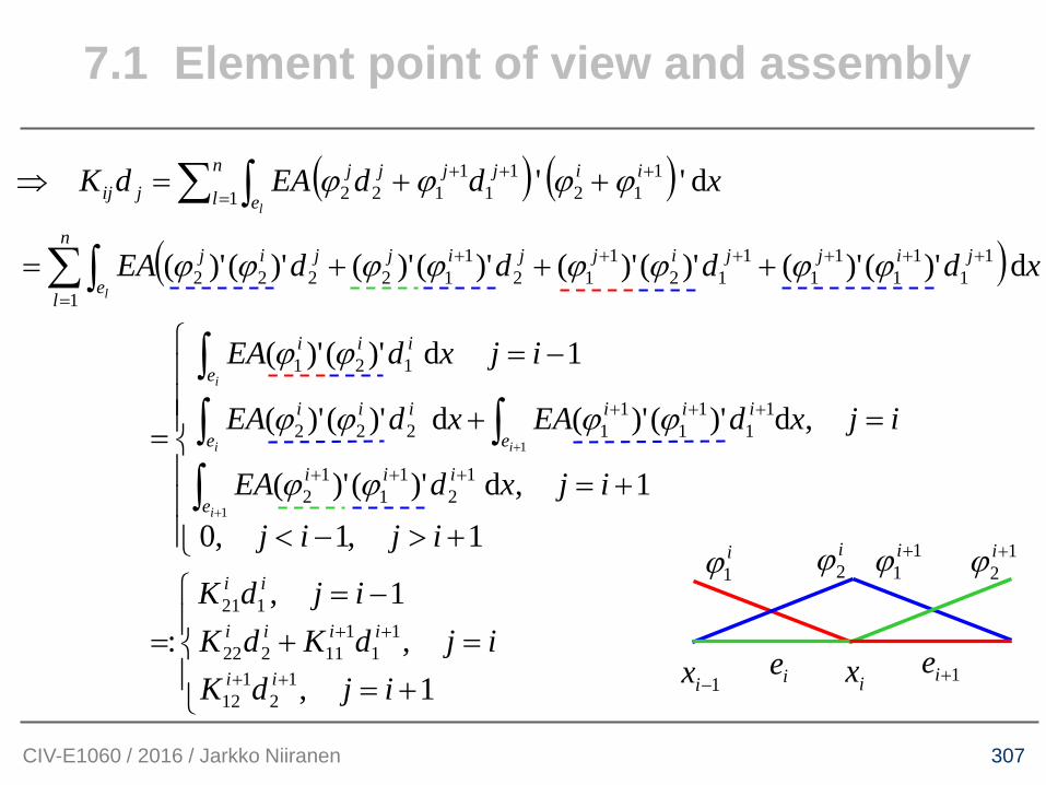
Second, let us consider the left hand side, the stiffness part:

renamed



307

( ) ( )

( )

+=

=+

−=

=

+−

+=

=+

−=

=

+++=

++=

++

++

+++

+++

=

++++++

=

+++

+

+

1,

,

1,

:

1,1,0

1,d)'()'(

,d)'()'(d)'()'(

1d)'()'(

d)'()'()'()'()'()'()'()'(

d''

1

2

1

12

1

1

1

11222

121

1

2

1

1

1

2

1

1

1

1

1

1222

121

1

1

1

1

1

1

1

1

12

1

12

1

12222

1

1

12

1

1

1

122

1

1

ijdK

ijdKdK

ijdK

ijij

ijxdEA

ijxdEAxdEA

ijxdEA

xddddEA

xddEAdK

ii

iiii

ii

e

iii

e

iii

e

iii

e

iii

n

le

jijjijjijjij

n

l e

iijjjj

jij

i

ii

i

l

l

ie

i

1i

2

1−ix ix 1+ie

1

1

+i 1

2

+i



309

Altogether, the global stiffness matrix and force vector (corresponding to the global

degrees of freedom vector), can be assembled from the element contributions:

T

L

nnnnniiii

i

nn

nnnn

nnnn

i

iiii

iiii

i

ij

NfffffffffffKufff

KK

KKKK

KKKK

K

KKKK

KKKK

KK

KKKK

KKK

K

++++++−+=

+

+

+

+

+

+

=

−−−+−

−−

−−−−

+

++

−−

−

21

1

2

1

1

2

2

1

121

1

2

3

1

2

2

1

210

2

1

1

2

2221

1211

1

22

1

21

1

12

1

11

2

22

2

21

1

21

1

12

1

112221

1211

1

22

1

21

1

12

3

21

3

12

3

11

2

22

2

21

2

12

2

11

1

22

0000

00

00

000

00

000

00

00

0000



310

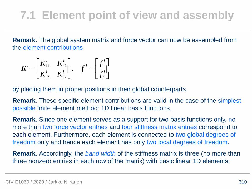
Remark. The global system matrix and force vector can now be assembled from

the element contributions

by placing them in proper positions in their global counterparts.

Remark. These specific element contributions are valid in the case of the simplest

possible finite element method: 1D linear basis functions.

Remark. Since one element serves as a support for two basis functions only, no

more than two force vector entries and four stiffness matrix entries correspond to

each element. Furthermore, each element is connected to two global degrees of

freedom only and hence each element has only two local degrees of freedom.

Remark. Accordingly, the band width of the stiffness matrix is three (no more than

three nonzero entries in each row of the matrix) with basic linear 1D elements.



11 12 1

12 22 2

,l l l

l l

l l l

K K f

K K f

= =

K f

311

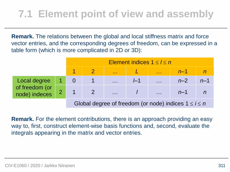
Remark. The relations between the global and local stiffness matrix and force

vector entries, and the corresponding degrees of freedom, can be expressed in a

table form (which is more complicated in 2D or 3D):

Remark. For the element contributions, there is an approach providing an easy

way to, first, construct element-wise basis functions and, second, evaluate the

integrals appearing in the matrix and vector entries.



Element indices 1 l n

1 2 ... L … n–1 n

Local degree

of freedom (or

node) indeces

1 0 1 … l–1 … n–2 n–1

2 1 2 … l … n–1 n

Global degree of freedom (or node) indices 1 i n

312

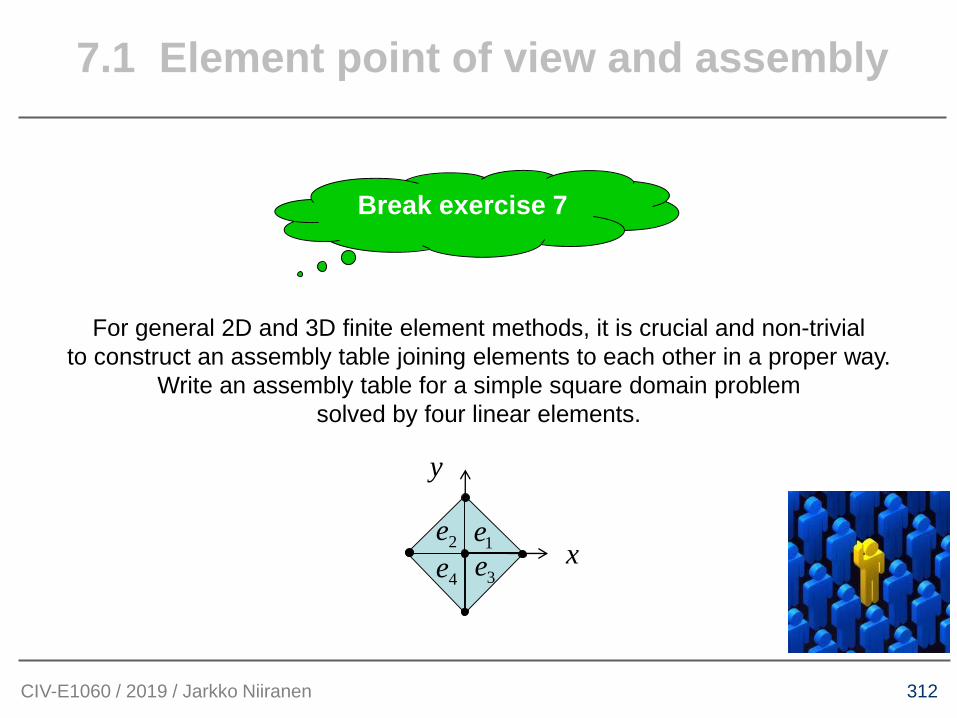
Break exercise 7

For general 2D and 3D finite element methods, it is crucial and non-trivial

to construct an assembly table joining elements to each other in a proper way.

Write an assembly table for a simple square domain problem

solved by four linear elements.



1e2e

3e4e

x

y

314

Finally, the local basis functions above (still functions of the local coordinate x) can

be expressed by using a local reference element with local reference basis functions

(of a local reference element coordinate ) and local degrees of freedom:

For local calculations, one needs to explicitly define the local basis functions (now

linear as the original global ones):

)(:)()(

)()()(

2211

2211

l

h

ll

llll

eh

udNdN

dxdxxul

=+=

+=


.2/1)('2/)1()(

2/1)('2/)1()(

22

11

=+=

−=−=

NN

NN

ie

1−i i

1−ix ix

1N 2N

1− 1refeie

i

1i

2

1−ix ix

renaming

1−

→ie

ie

F

F

7.2 Reference elements and coordinate

transformations

315

Remark. The trial solution of local (nodal) basis functions is now expressed in terms

of local (nodal) reference element basis functions visualized as follows:

i 1+i

ix 1+ix Lxn =00 =x

01

n

i 1+i

ix 1+ix Lxn =00 =x

01

n

1+ie

i 1+i

ix 1+ix

1N 2N

1− 1refe

1

1

1

−

+

+

→ie

ie

F

F1+ie

1

1

+i1

2

+i

ix 1+ix

renaming



transformations

316

Remark. The reference element ”serves” all elements:

= =

=

=

= −−

=

=

+=

+=

+=

=

n

l p

l

pp

n

l

ll

n

l

llll

n

l lellel

j

n

j jh

dN

dNdN

dxdx

dxdx

dxxu

ll

1

2

1

1 2211

1 2211

1 11

0

)(

)()(

)()(

)()(

)()(

1+ie

1

1

+i1

2

+i

ix 1+ix

renamed

1+ie

i 1+i

ix 1+ix

original

1N 2N

1− 1refe

reference

ie

iei 1−iei


original



transformations

318

Reference element mappings in 1D. Between the reference element (of the local

coordinate ) and the actual element (of the global coordinate x), one needs to

construct an (affine) transformation, or mapping, and its derivative, i.e.,

as well as the inverse as its derivative:

Remark. It is easy to check that the mapping transforms the reference element onto

the actual element, i.e, points are mapped to .

Remark. What is the geometrical meaning of the derivative of the mapping Fe?

11 ,

2)(',

2)(

,:

−− −==++

==

→

iiii

eiii

e

irefe

xxhh

Fxxh

Fx

eeF

ii

i


)('

12)()'(,

2)(

,:

111

1

i

ii

i

ei

e

i

iie

refie

FhxF

h

xxxxFx

eeF

==−−

==

→

−−−

−


transformations

1,0,1 = − 1 1, ( ) / 2,i i i ix x x x− −+

321

The local element force vector consist of two (2 x 1) entries following the construction

above:

Since all the element contributions to the global force vector have a common format,

it is practical to compute them by utilizing the reference element, by accomplishing a

change of variables in the integration:

2 0 21 1 1

1

2 0 21 1 11

1

01

( ) ( ) d ; 1,2

d( ( )) ( ) d ; ( )

d

1( ( )) (1 ) d , for 0, 0

2 2

b / 2, for constant

l

l i

l

l l l

p p L p nl p le

l

e p L p nl p l e

le L

l

f b x x x N u K p

xb F N N u K x F

hb F N u

h b

−

−

= + − =

= + − =

= = =

=

=

l

l

l

f

f

2

1f



transformations

324

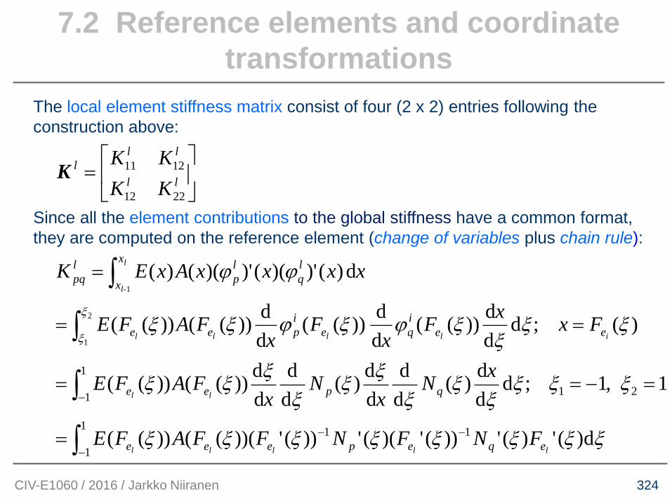
The local element stiffness matrix consist of four (2 x 2) entries following the

construction above:

Since all the element contributions to the global stiffness have a common format,

they are computed on the reference element (change of variables plus chain rule):

=

ll

ll

l

KK

KK

2212

1211K

−

−−

−

=

=−==

==

=

1

1

11

21

1

1

d)(')('))(')(('))('))((())((

1,1;dd

d)(

d

d

d

d)(

d

d

d

d))(())((

)(;dd

d))((

d

d))((

d

d))(())((

d)()')(()')(()(

2

1

1

lllll

ll

illll

l

l-

eqepeee

qpee

ee

i

qe

i

pee

x

x

l

q

l

p

l

pq

FNFNFFAFE

xN

xN

xFAFE

Fxx

Fx

Fx

FAFE

xxxxAxEK


transformations


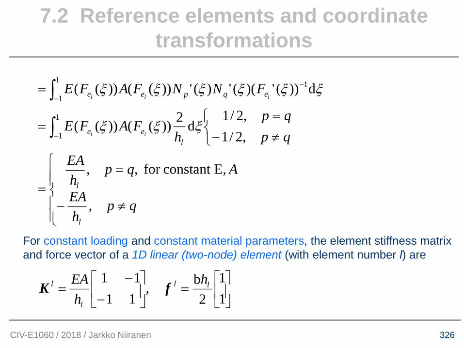
326

=

−

−=

1

1

2

b,

11

11ll

l

l h

h

EAfK

For constant loading and constant material parameters, the element stiffness matrix

and force vector of a 1D linear (two-node) element (with element number l) are

−

=

=

−

==

=

−

−

−

qph

EA

Aqph

EA

qp

qp

hFAFE

FNNFAFE

l

l

l

ee

eqpee

ll

lll

,

,constant Efor ,,

,2/1

,2/1d

2))(())((

d))(')((')('))(())((

1

1

1

1

1


transformations


327

Remark. For non-constant material parameters or loadings, the integrals appearing

in the matrix and vector entries of the reference element are computed with the aid of

a quadrature of numerical integration which is chosen according to the type of the

integrand.

Remark. The reference element stiffness matrix and force vector can be modified to

the needs of any problem having the same generic form as the bar problem: for heat

diffusion, for instance, EA is simply replaced by k and so on.

Remark. Similar local stiffness matrices and force vectors for the simples cases of

constant parameters can be derived for higher-order elements as well. The size of

the matrices and vector naturally depends on the number of nodes in the reference

element (see the Theoretical exercises): for the 1D quadratic (three-node) element,

the sizes are 3 x 3 (stiffness) and 3 x 1 (force) .

Remark. Much of the efficiency and adaptability of FEM comes from the reference

element concept and its implications to the computer implementations and the use of

the memory and processor units of computers (even up to parallelization).


transformations


329

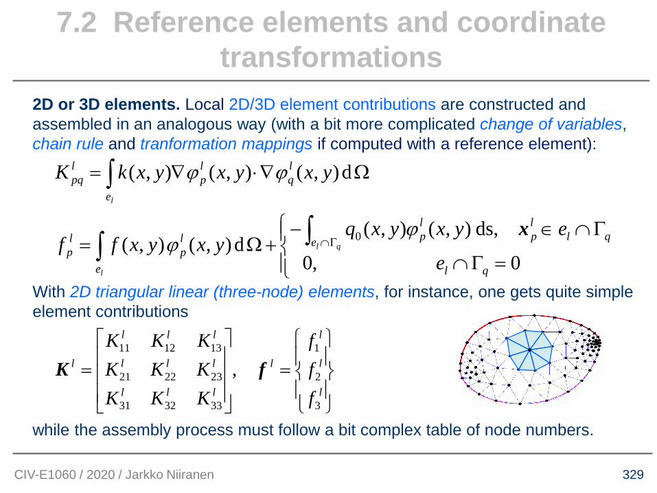
2D or 3D elements. Local 2D/3D element contributions are constructed and

assembled in an analogous way (with a bit more complicated change of variables,

chain rule and tranformation mappings if computed with a reference element):

With 2D triangular linear (three-node) elements, for instance, one gets quite simple

element contributions

while the assembly process must follow a bit complex table of node numbers.

=

−+=

=

0,0

,ds),(),(d),(),(

d),(),(),(

0

ql

ql

l

pe

l

p

e

l

p

l

p

e

l

q

l

p

l

pq

e

eyxyxqyxyxff

yxyxyxkK

ql

l

l

x

=

=l

l

l

l

lll

lll

lll

l

f

f

f

KKK

KKK

KKK

3

2

1

333231

232221

131211

, fK


transformations


331

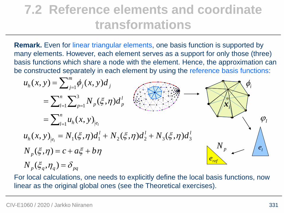
Remark. Even for linear triangular elements, one basis function is supported by

many elements. However, each element serves as a support for only those (three)

basis functions which share a node with the element. Hence, the approximation can

be constructed separately in each element by using the reference basis functions:

For local calculations, one needs to explicitly define the local basis functions, now

linear as the original global ones (see the Theoretical exercises).

pqqqp

p

lll

eh

n

l eh

n

l p

l

pp

j

m

j jh

N

bacN

dNdNdNyxu

yxu

dN

dyxyxu

l

l

=

++=

++=

=

=

=

=

= =

=

),(

),(

),(),(),(),(

),(

),(

),(),(

332211

1

1

3

1

1


transformations


ix

i

refe

le

l

pN

334

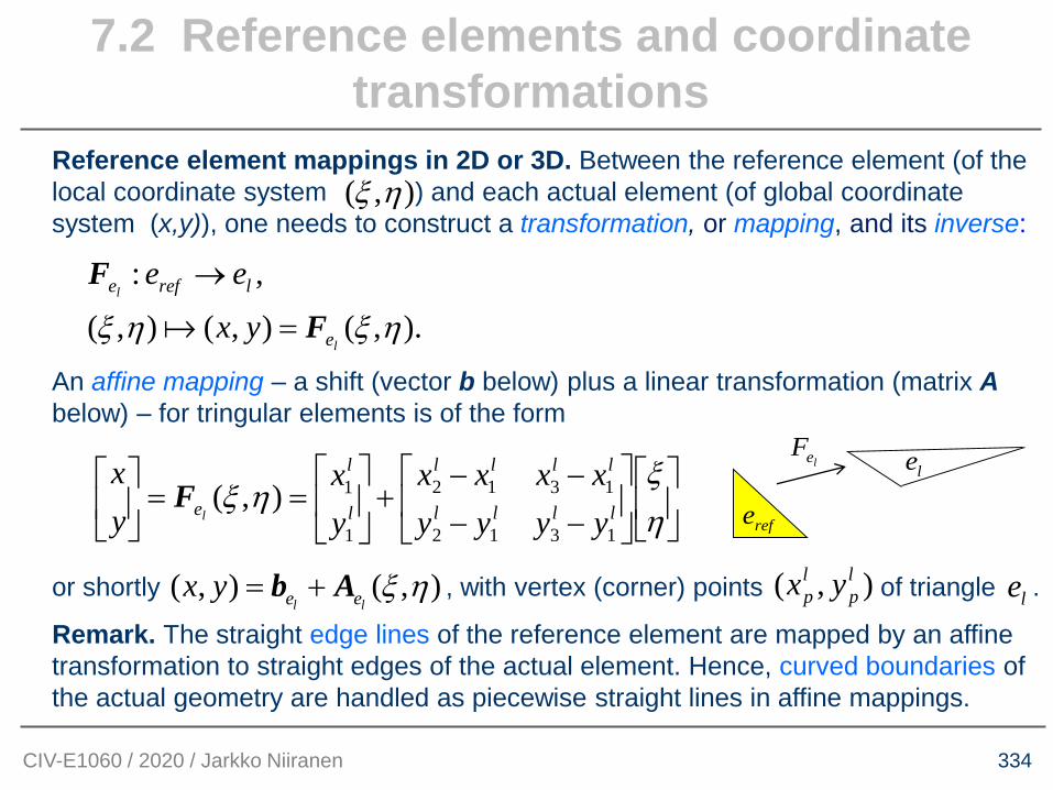
Reference element mappings in 2D or 3D. Between the reference element (of the

local coordinate system ) and each actual element (of global coordinate

system (x,y)), one needs to construct a transformation, or mapping, and its inverse:

An affine mapping – a shift (vector b below) plus a linear transformation (matrix A

below) – for tringular elements is of the form

or shortly , with vertex (corner) points of triangle .

Remark. The straight edge lines of the reference element are mapped by an affine

transformation to straight edges of the actual element. Hence, curved boundaries of

the actual geometry are handled as piecewise straight lines in affine mappings.

).,(),(),(

,:

l

l

e

lrefe

yx

ee

F

F

=

→

refe

leleF

−−

−−+

==

llll

llll

l

l

eyyyy

xxxx

y

x

y

xl

1312

1312

1

1),(F

),(

),( l

p

l

p yxle


transformations


( , ) ( , )l le ex y = +b A

335

Example. In a Master’s Thesis (Kimmo Ylinen, 2016: Crack Spacing in Reinforced

Concrete Members with Large Diameter Rebars and Thick Concrete Covers),

hexahedral (20-node) 3D elements were required even from the geometrical point of

view: for properly representing the curved geometry of the contact surfaces between

the rebars and concrete.

Simulations for an extension test:

- software package: Code_Aster

- symmetry conditions utilized

- method verification with different mesh sizes

- model validation versus an experimental test


transformations


https://www.code-aster.org/spip.php?rubrique2

336

The crack spacing from the FEM simulation quite well follows an experimental test:


transformations


337

Remark. Stiffness matrices are often written in literature in the form

including, even if the problem is not about displacements, strains and stresses, the

so-called strain-displacement matrix B consisting of shape function derivatives,

(assuming a linear triangle with three basis functions) whereas the so-called material

matrix, or constitutive matrix, D takes a simple diagonal form in isotropic heat

conduction:

In the problems of elasticity theory, the material matrix includes the corresponding

material parameters such as the Young’s modulus and Poisson’s ratio – but not in a

diagonal form (as will turn out).

dl

l T

e= K B D B


transformations


diag( )k=D

1 2 3,l l l l l T = = B Φ Φ

338

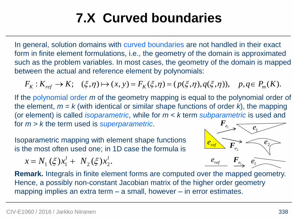
7.X Curved boundaries

In general, solution domains with curved boundaries are not handled in their exact

form in finite element formulations, i.e., the geometry of the domain is approximated

such as the problem variables. In most cases, the geometry of the domain is mapped

between the actual and reference element by polynomials:

If the polynomial order m of the geometry mapping is equal to the polynomial order of

the element, m = k (with identical or similar shape functions of order k), the mapping

(or element) is called isoparametric, while for m < k term subparametric is used and

for m > k the term used is superparametric.

Isoparametric mapping with element shape functions

is the most often used one; in 1D case the formula is

Remark. Integrals in finite element forms are computed over the mapped geometry.

Hence, a possibly non-constant Jacobian matrix of the higher order geometry

mapping implies an extra term – a small, however – in error estimates.

).(,)),,(),,((),(),(),(;: KPqpqpFyxKKF mKrefK ==→

refe

1e1eF

2e2eF

.)()( 2211

ll xNxNx += refeleF

le


QUESTIONS?

ANSWERS”

LECTURE BREAK!

Documents

7 Numerical implementation techniques of finite element