Embed Size (px)
Citation preview

NONLINEAR PROGRAMMINGPROGRAMMING
(Hillier & Lieberman Introduction to Operations Research, 8th edition)

Nonlinear Programmingg g
Linear programming has a fundamental role in ORLinear programming has a fundamental role in OR.In linear programming all its functions (objective f i d i f i ) lifunction and constraint functions) are linear.This assumption frequently does not hold, and nonlinear programming problems are formulated:Find x = (x1, x2,..., xn) to
Maximize f (x)subject to
gi(x) ≤ bi , for i = 1, 2, ..., mand x ≥ 0
João Miguel da Costa Sousa / Alexandra Moutinho 325

Nonlinear Programmingg g
There are many types of nonlinear programming There are many types of nonlinear programming problems, depending on f(x) and gi(x) – assumed differentiable or piecewise linear functionsdifferentiable or piecewise linear functions.Different algorithms are used for different types.Some problems can be solved very efficiently, whilst others, even small, can be very difficult.Nonlinear programming is a particularly large subject.jOnly some important types will be dealt with here. Some applications are give in the followingSome applications are give in the following.
João Miguel da Costa Sousa / Alexandra Moutinho 326

Application: product‐mix problempp p p
In product‐mix problems (as Wyndor Glass Co.) the goal is to determine optimal mix of production levels.Sometimes price elasticity is present: the amount of sold product has an inverse relation to price charged:
João Miguel da Costa Sousa / Alexandra Moutinho 327

Price elasticityy
p(x) is the price required to sell x units.p( ) p qc is the unit cost for producing and distributing product.Profit from producing and selling x is:o t o p oduc g a d se g s
P(x) = xp(x) – cx
João Miguel da Costa Sousa / Alexandra Moutinho 328

Product‐mix problemp
If each product has a similar profit function overall If each product has a similar profit function, overall objective function is
=
= ∑1
( ) ( )n
j jj
f x P x
Other nonlinearity: marginal cost varies with production level. p
It may decrease when production level is increased due to the learning‐curve effect.g ffIt may increase due to overtime or more expensive production facilities when production increases.
João Miguel da Costa Sousa / Alexandra Moutinho 329

Application: transportation problempp p p
Determine optimal plan for shipping goods from various sources to various destinations (see P&T Company problem).Cost per unit shippedmay not be fixed. Volume discounts are sometimes available for large shipments.Marginal cost can have a pattern like in the figure. Cost of shipping x units is a piecewise linear function Cost of shipping x units is a piecewise linear function C(x), with slope equal to the marginal cost.
João Miguel da Costa Sousa / Alexandra Moutinho 330

Volume discounts on shipping costspp g
Marginal cost Cost of shipping
João Miguel da Costa Sousa / Alexandra Moutinho 331

Transportation problemp p
If each combination of source and destination has a similar shipping cost function, so that cost of shipping xij units from source i (i = 1, 2, ..., m) to destination j (j = 1, 2, ..., n) is given by a nonlinear gfunction Cij(xij),the overall objective function ist e o e a object e u ct o s
= ∑∑Minimize ( ) ( )m n
ij ijf C xx= =∑∑1 1
( ) ( )ij iji j
f
João Miguel da Costa Sousa / Alexandra Moutinho 332

Graphical illustrationp
Example: Wyndor Glass Co. problem with NL constraint p y p
João Miguel da Costa Sousa / Alexandra Moutinho 333

Graphical illustrationp
Example: Wyndor Glass Co. with NL objective function p y j
João Miguel da Costa Sousa / Alexandra Moutinho 334

Example: Wyndor Glass Co. (3)p y (3)
João Miguel da Costa Sousa / Alexandra Moutinho 335

Global and local optimump
Example: f(x)with three local maxima (where?), and three local minima (where?). Global?
João Miguel da Costa Sousa / Alexandra Moutinho 336

Guaranteed local maximum
Global maximum when: ∂≤
∂
2
2( ) 0, for all f x
x
Function always “curving downward” is a concave function (concave downward).
∂ 2 ,x
Function always “curving upward” is a convex function (concave upward).
João Miguel da Costa Sousa / Alexandra Moutinho 337

Guaranteed local optimump
Nonlinear programming with no constraints and Nonlinear programming with no constraints and concave objective function, a local maximum is the global maximum.global maximum.Nonlinear programming with no constraints and convex objective function a local minimum is the convex objective function, a local minimum is the global minimum.With t i t th t till h ld if th With constraints, these guarantees still hold if the feasible region is a convex set.The feasible region for a NP problem is a convex set if all gi(x) are convex functions.
João Miguel da Costa Sousa / Alexandra Moutinho 338

Ex: Wyndor Glass with one concave gi(x)y gi( )
João Miguel da Costa Sousa / Alexandra Moutinho 339

Convex Programming problemg g p
To guarantee a local maximum is a global maximumfor a NP problemwith constraints gi(x) ≤ bi , for i = 1, 2, ..., m and x ≥ 0, the objective function f (x)must be a concave function and each gi(x) must be a convexfunction.See appendix 2 of Hillier’s book for convexityproperties and definitions.
João Miguel da Costa Sousa / Alexandra Moutinho 340

Types of NP problemsyp p
Unconstrained Optimization: no constraintsUnconstrained Optimization: no constraints
Maximize ( )f x
necessary condition for a solution x* = x to be optimal:∂
= = =*( ) 0 at for 1 2fj n
xx x
when f (x) is a concave function this condition is sufficient.
= = =∂
…0 at , for 1,2, ,j
j nx
x x
when xj has a constraint xj ≥ 0, sufficient condition changes to:
⎧≤∂ ⎪ * *0 t if 0( )f ⎧≤ = =∂ ⎪⎨= = >∂ ⎪⎩
* *
0 at , if 0( )0 at , if 0
j
jj
xfxx
x xxx x
João Miguel da Costa Sousa / Alexandra Moutinho 341

Example: nonnegative constraintp g
João Miguel da Costa Sousa / Alexandra Moutinho 342
Types of NP problemsyp p
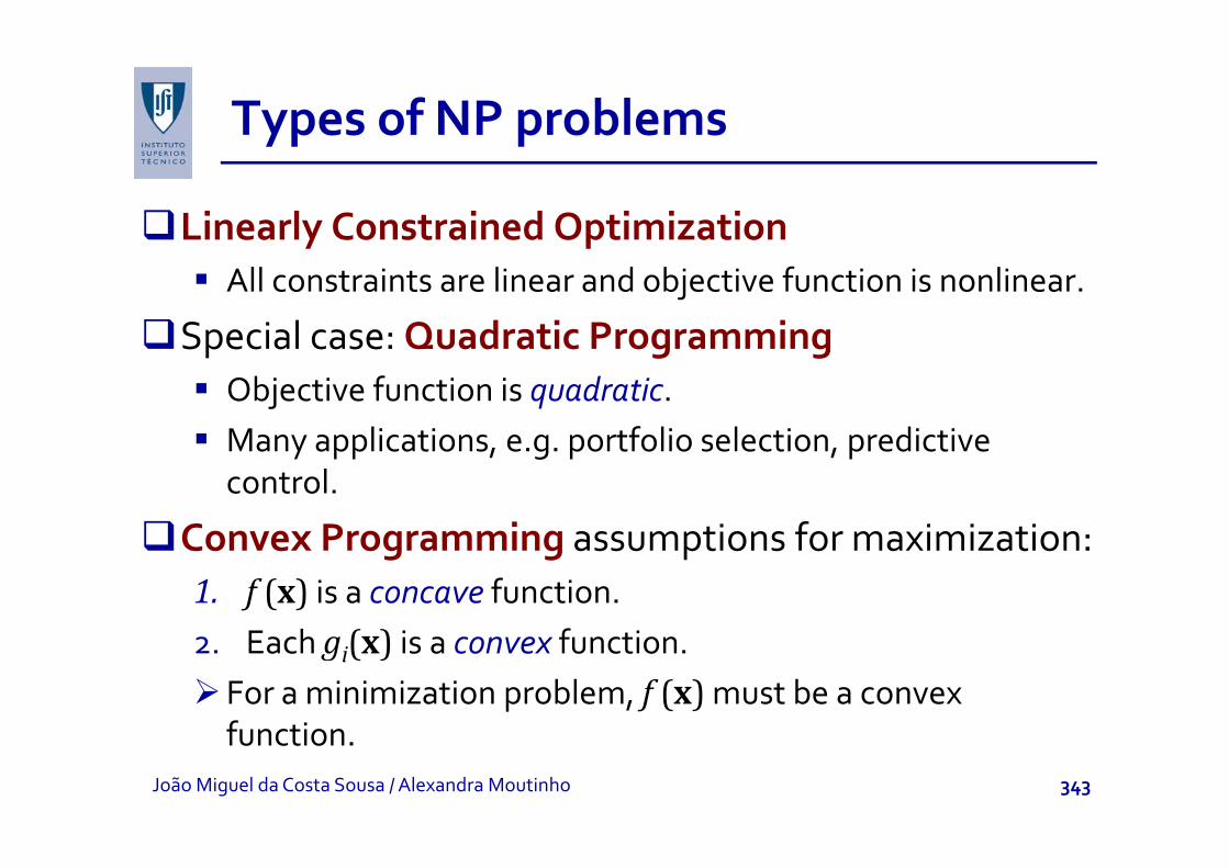
Linearly Constrained OptimizationLinearly Constrained OptimizationAll constraints are linear and objective function is nonlinear.
Special case: Quadratic ProgrammingSpecial case: Quadratic ProgrammingObjective function is quadratic.M li ti tf li l ti di ti Many applications, e.g. portfolio selection, predictive control.
Convex Programming assumptions for maximizationConvex Programming assumptions for maximization:1. f (x) is a concave function.
E h ( ) i f i2. Each gi(x) is a convex function.For a minimization problem, f (x)must be a convex functionfunction.
João Miguel da Costa Sousa / Alexandra Moutinho 343

Types of NP problemsyp p
Separable Programming is a special case of convex Separable Programming is a special case of convex programming with additional assumption3 All f(x) and gi(x) are separable functions3. All f(x) and gi(x) are separable functions.A separable function is a function where each term involves only a single variable (satisfies assumption of involves only a single variable (satisfies assumption of additivity but not proportionality):
n
=
= ∑1
( ) ( )n
j jj
f f xx
Nonconvex Programming: local optimum is not assured to be a global optimum. g p
João Miguel da Costa Sousa / Alexandra Moutinho 344

Types of NP problemsyp p
Geometric Programming is applied to engineering Geometric Programming is applied to engineering design as well as economics and statistics problems
Obj i f i d i f i f h fObjective function and constraint functions are of the form:
= =∑ 1 21 2( ) ( ), where ( ) i i in
Na a a
i i i ng c P P x x xx x x
ci and aij are typically physical constraints.=∑ 1 21
( ) ( ), ( )i i i ni
g
When all ci are strictly positive, functions are generalized positive polynomials (posynomials). If the objective function is to be minimized a convex programming function is to be minimized, a convex programming algorithm can be applied.
João Miguel da Costa Sousa / Alexandra Moutinho 345

Types of NP problemsyp p
Fractional Programming
= 1( )Maximize ( ) ff
xx
when f (x) has the linear fractional programming form:
=2
Maximize ( )( )
ff
xx
when f (x) has the linear fractional programming form:
+=
+0 ( ) c
fd
cxx
dxproblem can be transformed into a linear programming problem.
+ 0ddx
p
João Miguel da Costa Sousa / Alexandra Moutinho 346

One‐variable unconstrained optimizationp
Methods for solving unconstrained optimization with g ponly one variable x (n = 1), where the differentiable function f (x) is concave.f ( )Necessary and sufficient condition for optimum:
∂= =
∂*( ) 0 at .f x
x xx∂x
João Miguel da Costa Sousa / Alexandra Moutinho 347

Solving the optimization problemg p p
If f (x) is not simple, problem cannot be solved analytically.If not, search procedures can solve the problem numerically.yWe will describe two common search procedures:
Bisection methodBisection methodNewton’s method
João Miguel da Costa Sousa / Alexandra Moutinho 348

Bisection method
Since f (x) is concave, we know that:Since f (x) is concave, we know that:
> < *( ) 0 if ,df xx x> <
= = *
0 if ,
( ) 0 if
x xdxdf x
x x
< > *
0 if ,
( ) 0 if
x xdxdf x
x x
Can hold if 2nd derivative ≥0 for some (not all) values of x
< >0 if .x xdx
Can hold if 2 derivative ≥0 for some (not all) values of x.If derivative of x is positive, x is a lower bound of x*.If derivative of x is negative x is an upper bound of x*If derivative of x is negative, x is an upper bound of x .
João Miguel da Costa Sousa / Alexandra Moutinho 349

Bisection method
Notation:
′ = current trial solution,x*
*
current trial solution, = current lower bound on ,x
x x
ε
*
*
= current upper bound on , = error tolerance for .x x
x
In the bisection method, new trial solution is the id i t b t th t t b dmidpoint between the two current bounds.
João Miguel da Costa Sousa / Alexandra Moutinho 350

Algorithm of the Bisection Methodg
Initialization: Select ε. Find initial upper +
ppand lower bounds. Select initial trial as:
It ti
+′ =2
x xx
Iteration:
1. Evaluate =( ) at ',df x
x x1. Evaluate
2. If
at ,x xdx
′≥ =( ) 0, reset ,df x
x xdx
3. If ′≤ =( ) 0, reset ,df x
x xdx
dx
4. Select a new
Stopping rule: If stop Otherwise go to 1
+′ =2
x xx
ε− ≤2x xStopping rule: If stop. Otherwise, go to 1.ε≤2x xJoão Miguel da Costa Sousa / Alexandra Moutinho 351

Example p
Maximize = − −4 6( ) 12 3 2f x x x xMaximize ( ) 12 3 2f x x x x
João Miguel da Costa Sousa / Alexandra Moutinho 352

Solution
First two derivatives: = − −3 5( ) 12(1 )df xx x
dFirst two derivatives:
= − +2
2 42
( )
( ) 12(3 5 )
dxd f x
x x+2 12(3 5 )x xdx
Iteration df (x)/dx x x New x’ f (x’)
ε = 0.01
0 0 2 1 7.0000
1 –12 0 1 0.5 5.7812
2 +10 12 0 5 1 0 75 7 69482 +10.12 0.5 1 0.75 7.6948
3 +4.09 0.75 1 0.875 7.8439
4 –2.19 0.75 0.875 0.8125 7.8672
5 +1.31 0.8125 0.875 0.84375 7.8829
6 –0.34 0.8125 0.84375 0.828125 7.8815
7 +0 51 0 828125 0 84375 0 8359375 7 88397 +0.51 0.828125 0.84375 0.8359375 7.8839
João Miguel da Costa Sousa / Alexandra Moutinho 353

Solution
x* ≈ 0.8360.828125 < x* < 0.84375
Bisection method converges relatively slowlyBisection method converges relatively slowly.Only information about first derivative is being used.
fAdditional information can be obtained by using second derivative, as in Newton’s method.
João Miguel da Costa Sousa / Alexandra Moutinho 354
Newton’s method
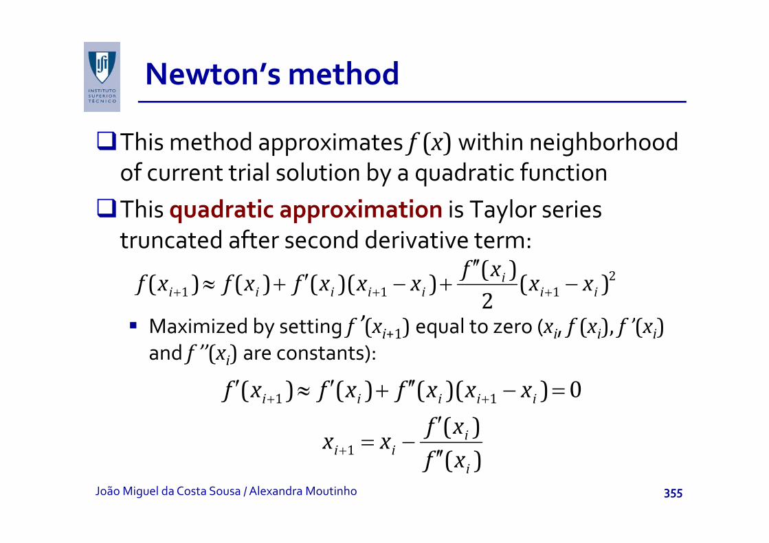
This method approximates f (x)within neighborhood This method approximates f (x)within neighborhood of current trial solution by a quadratic functionThis quadratic approximation is Taylor series This quadratic approximation is Taylor series truncated after second derivative term:
′′ 2( )f x
Maximized by setting f ’(xi+1) equal to zero (xi, f (xi), f ’(xi)+ + +′≈ + − + − 21 1 1
( )( ) ( ) ( )( ) ( )2
ii i i i i i i
f xf x f x f x x x x x
a ed by sett g f ( i+1) equa to e o ( i, f ( i), f ( i)and f ’’(xi) are constants):
′ ′ ′′≈ + − =1 1( ) ( ) ( )( ) 0i i i i if x f x f x x x+ +
+
≈ +′
= −′′
1 1
1
( ) ( ) ( )( ) 0( ) ( )
i i i i i
ii i
f x f x f x x x
f xx x
f x′′( )if xJoão Miguel da Costa Sousa / Alexandra Moutinho 355

Algorithm of Newton’s Methodg
Initiali ation Select Find initial trial sol tion b Initialization: Select ε. Find initial trial solution xi by inspection. Set i = 1.Iteration i:
1. Calculate f ’(xi) and f ’’(xi).2. Set
′( )if xx x
l f | | l
+ = −′′1 .( )i i
i
x xf x
Stopping rule: If |xi+1 ‐ xi | ≤ ε, stop; xi+1 is optimal. Otherwise, i = i + 1 (another iteration).
João Miguel da Costa Sousa / Alexandra Moutinho 356

Example p
M i i i 4 6( ) 12 3 2fMaximize againNew solution is given by:
= − −4 6( ) 12 3 2f x x x x
+
′ − − − −= − = − = +
′′ − + +
3 5 3 5
1 2 4 2 4( ) 12(1 ) 1 ( ) 12(3 5 ) 3 5
i i i i ii i i i
i i i i i
f x x x x xx x x x
f x x x x x
Selecting x1 = 1, and ε = 0.00001:( ) ( )i i i i if
Iteration i xi f (xi) f ’(xi) f ’’(xi) xi+11 1 7 –12 –96 0.875
8 8 6 82 0.875 7.8439 –2.1940 –62.733 0.84003
3 0.84003 7.8838 –0.1325 –55.279 0.83763
4 0.83763 7.8839 –0.0006 –54.790 0.83762
João Miguel da Costa Sousa / Alexandra Moutinho 357

Multivariable unconstrained optimizationp
Problem: maximizing a concave function f (x) of multiple variables x = (x1, x2,..., xn) with no constraints.Necessary and sufficient condition for optimality: partial derivatives equal to zero.No analytical solution → numerical search procedure must be used.ust be usedOne of these is the gradient search procedure:
It identifies and uses the direction of movement from the It identifies and uses the direction of movement from the current trial solution that maximizes the rate at which f (x)is increased.
João Miguel da Costa Sousa / Alexandra Moutinho 358

Gradient search procedurep
Use values of partial derivatives to select the specific Use values of partial derivatives to select the specific direction to move, using the gradient.G di f i ’ i h i h i lGradient of a point x = x’ is the vectorwith partial derivatives evaluated at x = x’:
⎛ ⎞∂ ∂ ∂′ ′∇ = =⎜ ⎟∂ ∂ ∂⎝ ⎠…
1 2
( ) , , , at n
f f ff
x x xx x x
Moves in the direction of this gradient until f (x) stops increasing Each iteration changes the trial solution
⎝ ⎠1 2 n
increasing. Each iteration changes the trial solution x’: ′ ′ ′= + ∇*Reset ( )t fx x x
João Miguel da Costa Sousa / Alexandra Moutinho 359

Gradient search procedurep
where t* is value of t ≥ 0 that maximizes f (x´ + t ∇f(x´)):where t is value of t ≥ 0 that maximizes f (x + t ∇f(x )):
′ ′ ′ ′+ ∇ = + ∇* ( ( )) max ( ( ))f t f f t fx x x x
The function f (x´ + t ∇f(x´)) is simply f (x)where:
≥0( ( )) ( ( ))
tf f f f
⎛ ⎞∂′= + =⎜ ⎟⎜ ⎟∂⎝ ⎠…, for 1,2, ,j j
fx x t j n
x
Iterations continue until ∇f (x) = 0 within ε tolerance:′=
⎜ ⎟∂⎝ ⎠jx x x
ε∂≤ =
∂…, for 1,2, , .
j
fj n
x∂ jx
João Miguel da Costa Sousa / Alexandra Moutinho 360

Summary of gradient search procedurey g p
Initialization: Select ε and any initial trial solution x’. Go to stopping rule.Iteration:
1. Express f (x´ + t∇f (x´)) as a function of t by setting1. Express f (x t∇f (x )) as a function of t by setting
⎛ ⎞∂′ + ⎜ ⎟ for 1 2fx x t j n
′=
= + =⎜ ⎟⎜ ⎟∂⎝ ⎠…, for 1,2, ,j j
j
fx x t j n
xx x
and substitute these expressions into f (x).
João Miguel da Costa Sousa / Alexandra Moutinho 361

Summary of gradient search procedurey g p
Iteration (concl.):2. Use search procedure to find t = t* that maximizesp
f (x’ + t ∇f(x’)) over t ≥ 0.3. Reset x’ = x’ + t* ∇f (x’). Go to stopping rule.3. Reset x x t ∇f (x ). Go to stopping rule.
Stopping rule: Evaluate ∇f(x’) at x = x’. Check if:∂f ε∂
≤ =∂
…, for 1,2, , .j
fj n
x
If so, stop with current x’ as the approximation of x*. Otherwise, perform another iteration.
João Miguel da Costa Sousa / Alexandra Moutinho 362

Example p
Maximize Thus,
= + − −2 21 2 2 1 2( ) 2 2 2 .f x x x x xx
∂ 2 2f= −
∂
∂
2 11
2 2fx x
x
f
V if th t f ( ) i ( A di f Hilli ’
∂= + −
∂ 1 22
2 2 4fx x
x
Verify that f (x) is concave (see Appendix 2 of Hillier’s book).Suppose that x = (0, 0) is initial trial solution. Thus,
∇ =(0,0) (0,2)f ( , ) ( , )f
João Miguel da Costa Sousa / Alexandra Moutinho 363
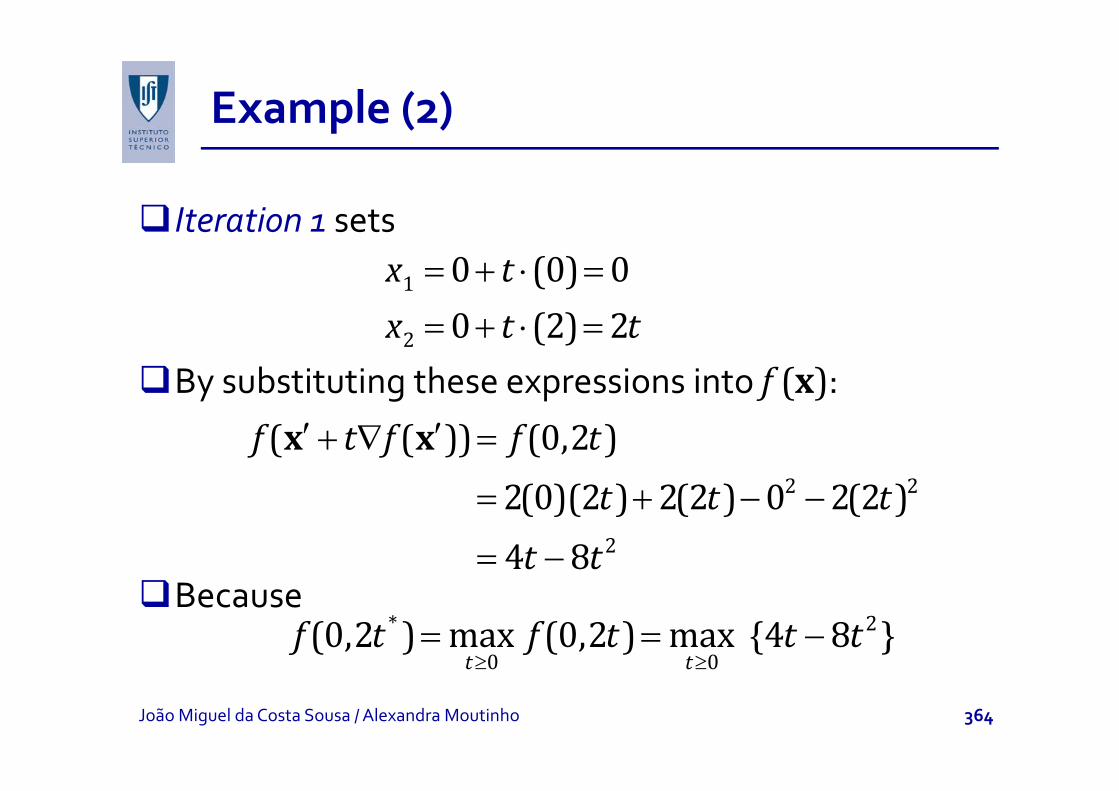
Example (2)p ( )
Iteration 1 setsIteration 1 sets= + ⋅ =1 0 (0) 0x t
By substituting these expressions into f (x):= + ⋅ =2 0 (2) 2x t t
y g p f ( )′ ′+ ∇ =
2 2
( ( )) (0,2 )2(0)(2 ) 2(2 ) 0 2(2 )
f t f f tx x
= + − −
= −
2 2
2
2(0)(2 ) 2(2 ) 0 2(2 )4 8
t t t
t tBecause
≥ ≥= = −* 2
0 0 (0,2 ) max (0,2 ) max {4 8 }
t tf t f t t t
≥ ≥0 0t t
João Miguel da Costa Sousa / Alexandra Moutinho 364

Example (3)p (3)
dand ( )− = − =24 8 4 16 0dt t t
dt1
it follows thatso
=* 14
t
⎛ ⎞1 1so
Thi l t fi t it ti F t i l di t
⎛ ⎞′ = + = ⎜ ⎟⎝ ⎠
1 1Reset (0,0) (0,2) 0,4 2
x
This completes first iteration. For new trial, gradient is:
⎛ ⎞∇ ⎜ ⎟10 (1 0)f∇ =⎜ ⎟
⎝ ⎠0, (1,0)2
f
João Miguel da Costa Sousa / Alexandra Moutinho 365

Example (4)p (4)
As ε < 1, Iteration 2:⎛ ⎞ ⎛ ⎞⎛ ⎞ ⎛ ⎞= + =⎜ ⎟ ⎜ ⎟⎝ ⎠ ⎝ ⎠
1 10, (1,0) ,2 2
t tx
so ⎛ ⎞ ⎛ ⎞′ ′+ ∇ = + + =⎜ ⎟ ⎜ ⎟⎝ ⎠ ⎝ ⎠
1 1 ( ( )) 0 , 0 ,2 2
f t f f t t f tx x⎝ ⎠ ⎝ ⎠
⎛ ⎞ ⎛ ⎞ ⎛ ⎞= + − −⎜ ⎟ ⎜ ⎟ ⎜ ⎟⎝ ⎠ ⎝ ⎠ ⎝ ⎠
221 1 1(2 ) 2 2
2 2 2t t⎜ ⎟ ⎜ ⎟ ⎜ ⎟
⎝ ⎠ ⎝ ⎠ ⎝ ⎠
= +2
( )2 2 21
t t= − +2
t t
⎛ ⎞ ⎛ ⎞ ⎧ ⎫= = − +⎨ ⎬⎜ ⎟ ⎜ ⎟21 1 1*, max , maxf t f t t t
≥ ≥+⎨ ⎬⎜ ⎟ ⎜ ⎟
⎝ ⎠ ⎝ ⎠ ⎩ ⎭0 0 , max , max
2 2 2t tf t f t t t
João Miguel da Costa Sousa / Alexandra Moutinho 366

Example (5)p (5)
⎛ ⎞ ⎛ ⎞ ⎧ ⎫* 21 1 1Because≥ ≥
⎛ ⎞ ⎛ ⎞ ⎧ ⎫= = − +⎨ ⎬⎜ ⎟ ⎜ ⎟⎝ ⎠ ⎝ ⎠ ⎩ ⎭
* 2
0 0
1 1 1 , max , max2 2 2t t
f t f t t t
⎛ ⎞dand ⎛ ⎞− + = − =⎜ ⎟⎝ ⎠
2 1 1 2 02
dt t t
dt
then =* 12
t
so ⎛ ⎞ ⎛ ⎞′ = + =⎜ ⎟ ⎜ ⎟⎝ ⎠ ⎝ ⎠
1 1 1 1Reset 0, (1,0) ,2 2 2 2
x
This completes second iteration. See figure.
⎜ ⎟ ⎜ ⎟⎝ ⎠ ⎝ ⎠2 2 2 2
João Miguel da Costa Sousa / Alexandra Moutinho 367

Illustration of examplep
Optimal solution is (1 1) as ∇f (1 1) (0 0)Optimal solution is (1, 1), as ∇f (1, 1) = (0, 0)
João Miguel da Costa Sousa / Alexandra Moutinho 368
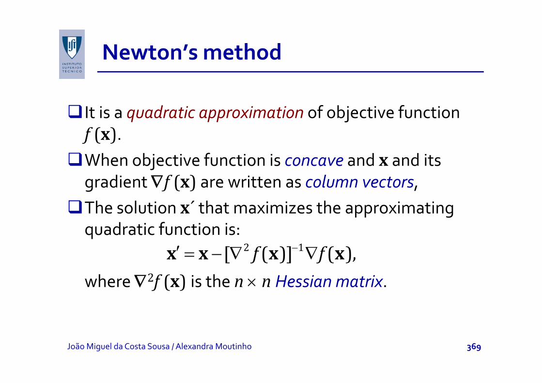
Newton’s method
It is a quadratic approximation of objective function f (x).When objective function is concave and x and its gradient ∇f (x) are written as column vectors, gThe solution x´ that maximizes the approximating quadratic function is:quad at c u ct o s
here ∇2f (x) is the n n Hessian matri
−′ = − ∇ ∇2 1[ ( )] ( ),f fx x x x
where ∇2f (x) is the n × n Hessian matrix.
João Miguel da Costa Sousa / Alexandra Moutinho 369

Newton’s method
The inverse of the Hessian matrix is commonly approximated in various ways.Approximations of Newton’s methods are referred to as quasi‐Newton methods (or variable metric methods).Recall that this topic was mentioned in Intelligent eca t at t s top c as e t o ed te ge tSystems, e.g. in neural network leaning.
João Miguel da Costa Sousa / Alexandra Moutinho 370

Conditions for optimalityp y
ProblemNecessary conditions
for optimalityAlso sufficient if:
One‐variable unconstrained f (x) concave=0dfdx
∂fMultivariable unconstrained f (x) concave
∂= =
∂…0, 1,2, ,
j
fj n
x
∂fConstrained, nonnegative constraints only f (x) concave
∂= =
∂≤ =
…0, 1,2, ,
(or 0, if 0)j
j
fj n
xx
General constrained problem Karush‐Kuhn‐Tucker conditionsf (x) concave and gi(x)convex ( i = 1, 2,..., m)
João Miguel da Costa Sousa / Alexandra Moutinho 371

Karush‐Kuhn‐Tucker conditions
Theorem: Assume that f(x), g1(x), g2(x),..., gm(x) are differentiable functions satisfying certain regularity conditions. Then
x = (x1*, x2*,..., xn*)can be an optimal solution for the NP problem if there are m numbers u1, u2,..., um such that all the KKT conditions are satisfied:
1.=
⎫∂ ∂− ≤ ⎪∂ ∂ ⎪
⎬
∑1
*
0m
ii
ij j
f gu
x x
2.
⎪ = =⎬⎛ ⎞∂ ∂ ⎪− =⎜ ⎟⎜ ⎟ ⎪∂ ∂⎝ ⎠ ⎭∑
…*
*
1
at , for 1,2 , .0
j j
mi
j ii
j nf g
x ux x
x x
=∂ ∂⎝ ⎠ ⎭1ij jx x
João Miguel da Costa Sousa / Alexandra Moutinho 372

Karush‐Kuhn‐Tucker conditions
⎫⎪*( ) 0b3.
4.
⎫− ≤ ⎪ =⎬− = ⎪⎭
…*
*
( ) 0for 1,2, , .
[ ( ) ] 0i i
i i i
g bj n
u g b
x
x
5.6
⎭
≥ =0 for 1 2u i m≥ = …* 0, for 1,2, , .jx j n
6.Conditions 2 and 4 require that one of the two q antities m st be ero
≥ …0, for 1,2, , .iu i m
quantities must be zero. Thus, conditions 3 and 4 can be combined:
(3,4) − =≤ = = …
*( ) 0(or 0, if 0), for i 1,2, , .
i i
i
g bu m
x
João Miguel da Costa Sousa / Alexandra Moutinho 373

Karush‐Kuhn‐Tucker conditions
Similarly, conditions 1 and 2 can be combined:
(1 2) ∂ ∂=∑ 0
mif g
u(1,2)=
− =∂ ∂
≤ = =
∑…
1*
0
(or 0 if 0), for 1,2 , .
iij j
j
ux x
x j n
Variables ui correspond to dual variables in linear
( )j j
Variables ui correspond to dual variables in linear programming.
Previous conditions are necessary but not sufficient to ensure optimality (see slide 371).
João Miguel da Costa Sousa / Alexandra Moutinho 374

Karush‐Kuhn‐Tucker conditions
Corollary: assume that f(x) is concave and g (x) Corollary: assume that f(x) is concave and g1(x), g2(x),..., gm(x) are convex functions, where all functions satisfy the regularity conditions Then x =functions satisfy the regularity conditions. Then, x = (x1*, x2*,..., xn*) is an optimal solution if and only if all the conditions of the theorem are satisfiedthe conditions of the theorem are satisfied.
João Miguel da Costa Sousa / Alexandra Moutinho 375

Examplep
= + +1 2Maximize ( ) ln( 1)f x xxsubject toj
+ ≤1 22 3x xand
≥ ≥1 20, 0x x
Thus m = 1 and g (x) = 2x + x is convexThus, m = 1, and g1(x) = 2x1 + x2 is convex.Further, f(x) is concave (check it using Appendix 2).Thus, any solution that verifies the KKT conditions is an optimal solution.
João Miguel da Costa Sousa / Alexandra Moutinho 376

Example: KKT conditionsp
1. (j = 1) − ≤11 2 01
u
(j = 2)+1 1x
− ≤11 0u
2. (j = 1) ⎛ ⎞− =⎜ ⎟+⎝ ⎠
1 11 2 01
x ux
(j = 2)+⎝ ⎠1 1x
( )− =2 11 0x u
3.
4+ − ≤1 22 3 0x x
+ − =(2 3) 0u x x4.5.6
+ =1 1 2(2 3) 0u x x
≥ ≥1 20, 0x x
06. ≥1 0uJoão Miguel da Costa Sousa / Alexandra Moutinho 377
Example: solving KKT conditionsp g
From condition 1 (j = 2) u1 ≥ 1; x1 ≥ 0 from condition 5Therefore, − <1
1 2 0.u,
Therefore, x1 = 0, from condition 2 (j = 1).0 i li h 2 3 0 f di i
+ 11 1x
u1 ≠ 0 implies that 2x1 + x2 – 3 = 0 from condition 4.Two previous steps implies that x2 = 3.x2 ≠ 0 implies that u1 = 1 from condition 2 (j = 2).No conditions are violated for x1 = 0 x2 = 3 u1 = 1No conditions are violated for x1 = 0, x2 = 3, u1 = 1.Consequently x* = (0,3).
João Miguel da Costa Sousa / Alexandra Moutinho 378

Quadratic Programmingg g
1= −
1Maximize ( )2
Tf x cx x Qxsubject toj
≤ ≥, andAx b x 0
Objective function can be expressed as:
∑ ∑∑1 1( )n n n
Tf c x q x xx cx x Qx= = =
= − = −∑ ∑∑1 1 1
( )2 2j j ij i j
j i j
f c x q x xx cx x Qx
João Miguel da Costa Sousa / Alexandra Moutinho 379

Examplep
+ + 2 2Maximize ( ) 15 30 4 2 4f x x x x x xx = + + − −1 2 1 2 1 2Maximize ( ) 15 30 4 2 4f x x x x x xx
subject to
In this case,
+ ≤ ≥ ≥1 2 1 22 30, and 0, 0x x x x
,
−⎡ ⎤ ⎡ ⎤= = =⎢ ⎥ ⎢ ⎥
1 4 4[15 30]
xc x Q= = =⎢ ⎥ ⎢ ⎥−⎣ ⎦⎣ ⎦2
[15 30]4 8x
c x Q
= =[1 2] [30]A b
João Miguel da Costa Sousa / Alexandra Moutinho 380

Solving QP problemsg p
Obj i f i i if TQ 0 i Q i Objective function is concave if xTQx 0 x, i.e., Q is a positive semidefinite matrix.
Some KKT conditions for quadratic programmingf q p g gproblems can be transformed in equality constraints by introducing slack variables (y1, y2, u1).y g y1, y2, 1
KKT conditions can be condensed due to the complementary variables ((x1, y1), (x2, y2), (u1, v1)), complementary variables ((x1, y1), (x2, y2), (u1, v1)), introducing complementary constraint (1+2+4).
João Miguel da Costa Sousa / Alexandra Moutinho 381

Solving QP problemsg p
Applying KKT conditions to exampleApplying KKT conditions to example1. (j = 1) 15+4x2‐4x1‐u1 ≤ 0
( 2) 30 4 8 2 0(j = 2) 30+4x1‐8x2‐2u1 ≤ 02. (j = 1) x1(15+4x2‐4x1‐u1) = 0
(j = 2) x2(30+4x1‐8x2‐2u1) = 03 x1+2x2‐30 ≤ 03. x1+2x2 30 ≤ 04. u1(x1+2x2‐30)=05. x1 x26. u1
João Miguel da Costa Sousa / Alexandra Moutinho 382

Solving QP problemsg p
(j 1) 4 4 151. (j = 1) ‐4x1+4x2‐u1+y1 = ‐15(j = 2) 4x1‐8x2‐2u1+y2 = ‐30
2. (j = 1) x1 y1 = 0(j = 2) x2 y2 = 0(j 2) x2 y2 0
3. x1+2x2+v1=3004. u1 v1 = 0
Complementar2 (j=1)+2 (j=2)+4. x1 y1 x2 y2 u1 v1
Complementaryconstraint
João Miguel da Costa Sousa / Alexandra Moutinho 383

Solving QP problemsg p
4x1‐4x2+u1‐y1 = 151 2 1 y1‐4x1+8x2+2u1‐y2 = 30x +2x +v =30
linear programming
x1+2x2+v1=30x1 x2 u1 y1 y2 v1
constraints
x1 y1 x2 y2 u1 v1
T T
T T
João Miguel da Costa Sousa / Alexandra Moutinho 384

Solving QP problemsg p
Using the previous properties, QP problems can be solved using a modified simplex method.See example of a QP problem in Hillier’s book (pages 580‐581).Excel, LINGO, LINDO, and MPL/CPLEX can all solve quadratic programming problems.quad at c p og a g p ob e s
João Miguel da Costa Sousa / Alexandra Moutinho 385

Separable Programmingp g g
Assumed that f(x) is concave and gi(x) are convex.
∑( ) ( )n
f f
f(x) is a (concave) piecewise linear function (see =
= ∑1
( ) ( )j jj
f f xx
f(x) is a (concave) piecewise linear function (see example).If (x) li thi bl b f l t d If gi(x) are linear, this problem can be reformulated as an LP problem by using a separate variable for each line segmenteach line segment.The same technique can be used for nonlinear gi(x).
João Miguel da Costa Sousa / Alexandra Moutinho 386

Examplep
João Miguel da Costa Sousa / Alexandra Moutinho 387

Examplep
João Miguel da Costa Sousa / Alexandra Moutinho 388

Convex Programmingg g
Many algorithms can be used, falling into 3 y g , g 3categories:
1. Gradient algorithms, where the gradient search g , gprocedure is modified to avoid violating a constraint.
Example: generalized reduced gradient (GRG).
2. Sequential unconstrained algorithms, includes penalty function and barrier functionmethods.
Example: sequential unconstrained minimization technique (SUMT).
i l i i l i h l d3. Sequential approximation algorithms, includes linear and quadratic approximationmethods.
E l F k W lf l i h f li iExample: Frank‐Wolfe algorithm for linear constraints.João Miguel da Costa Sousa / Alexandra Moutinho 389

Frank‐Wolfe algorithmg
It is a sequential linear approximation algorithm. It replaces the objective function f(x) by the first‐p j yorder Taylor expansion of f(x) around x = x´, namely:
′∂ ′∑ ( )n f x
A f(x´) d ∇f(x´)x´ h fi d l th b =
∂ ′′ ′ ′ ′ ′≈ + − = + ∇ −∂∑
1
( )( ) ( ) ( ) ( ) ( )( )j jj j
ff f x x f f
xx
x x x x x x
As f(x ) and ∇f(x )x have fixed values, they can be dropped to give equivalent linear objective function:
∂ ( )n f
=
∂′ ′= ∇ = = =∂∑
1
( )( ) ( ) , where at .n
j j jj j
fg f c x c
xx
x x x x x
João Miguel da Costa Sousa / Alexandra Moutinho 390

Frank‐Wolfe algorithmg
Simplex method is applied to find a solution xLP.Then, chose the point that maximizes the nonlinear pobjective function along the line segment.This can be done using an one‐variable unconstrained This can be done using an one variable unconstrained optimization algorithm.The algorithm continues the iterations until the stop The algorithm continues the iterations until the stop condition is satisfied.
João Miguel da Costa Sousa / Alexandra Moutinho 391

Summary of Frank‐Wolfe algorithmy g
( )Initialization: Find feasible initial trial solution x(0), e.g. using LP to find initial BF solution. Set k = 1.Iteration k:
1. For j = 1, 2, ..., n, evaluate ( 1)( )at .kf −∂
=x
x x1. For j 1, 2, ..., n, evaluateand set cj equal to this value.
2 Find optimal solution by solving LP problem:
jx∂
( )kx2. Find optimal solution by solving LP problem:LPx
Maximize ( ) ,n
j jg c x= ∑x
subject to
and≤ ≥Ax b x 0
1j=
and≤ ≥Ax b x 0João Miguel da Costa Sousa / Alexandra Moutinho 392

Summary of Frank‐Wolfe algorithmy g
3. For the variable t ∈ [0,1], set( 1) ( ) ( 1)
LP LP( ) ( ) for ( ),k k kh t f t− −= = + −x x x x x
so that h(t) gives value of f(x) on line segment between (where t = 0) and (where t = 1).
LP LP
( 1)k−x ( )LPkxbetween (where t 0) and (where t 1).
Use one‐variable unconstrained optimization to maximize h(t) to find x(k)
LP
maximize h(t) to find x( ).Stopping rule: If x(k–1) and x(k) are sufficiently close stop x(k) is the estimate of optimal solution stop. x(k) is the estimate of optimal solution. Otherwise, reset k = k + 1.
João Miguel da Costa Sousa / Alexandra Moutinho 393

Examplep
2 2Maximize ( ) 5 8 2f x x x x= +x 1 1 2 2Maximize ( ) 5 8 2f x x x x= − + −x
subject tod
h
1 2 1 23 2 6, and 0, 0x x x x+ ≤ ≥ ≥
Note that
5 2 8 4f f
x x∂ ∂
so that the unconstrained maximum x = (2 5 2)
1 21 2
5 2 , 8 4x xx x
= − = −∂ ∂
so that the unconstrained maximum x = (2.5, 2) violates the functional constraint.
João Miguel da Costa Sousa / Alexandra Moutinho 394

Example (2)p ( )
Iteration 1: x = (0, 0) is feasible (initial trial x(0)). Step 1 gives c1 = 5 and c2 = 8, so g(x) = 5x1 + 8x2.Step 2: solving graphically yields = (0, 3).Step 3: points between (0, 0) and (0, 3) are:
(1)LPx
Step 3: points between (0, 0) and (0, 3) are:
1 2( , ) (0,0) [(0,3) (0,0)] for [0,1](0 3 )
x x t tt
= + − ∈=
This expression gives
(0,3 )t=
2
2
( ) (0,3 ) 8(3 ) 2(3 )24 18
h t f t t tt t
= = −= −
João Miguel da Costa Sousa / Alexandra Moutinho 395
Example (3)p (3)
the value t = t* that maximizes h(t) is given by( )
24 36 0dh t
t= − =
so t* = 2/3. This results leads to the next trial solution,
24 36 0tdt
= − =
3 ,(see figure):
(1) 2(0,0) [(0,3) (0,0)]= + −x
It ti f ll i th d l d t th
3(0,2)=
Iteration 2: following the same procedure leads to the next trial solution x(2) =(5/6, 7/6).
João Miguel da Costa Sousa / Alexandra Moutinho 396

Example (4)p (4)
João Miguel da Costa Sousa / Alexandra Moutinho 397

Example (5)p (5)
Figure shows next iterations.Note that trial solutions alternate between two trajectories that intersect at point x = (1, 1.5).This is the optimal solution (satisfies KKT conditions).This is the optimal solution (satisfies KKT conditions).
Using q adratic instead of linear appro imations lead Using quadratic instead of linear approximations lead to a much faster convergence.
João Miguel da Costa Sousa / Alexandra Moutinho 398

Sequential unconstrained minimizationq
Main versions of SUMT Main versions of SUMT: exterior‐point algorithm: deals with infeasible solutions and a penalty function a penalty function, interior‐point algorithm: deals with feasible solutions and a barrier function barrier function.
Uses the advantage of solving unconstrained problems which are much easier to solve problems, which are much easier to solve. Each unconstrained problem in the sequence chooses ll d ll l f d l f ta smaller and smaller value of r, and solves for x to
Maximize ( ; ) ( ) ( )P r f rB= −x x x
João Miguel da Costa Sousa / Alexandra Moutinho 399

SUMT
B(x) is a barrier functionwith following properties (for feasible x for original problem):1. B(x) is smallwhen x is far from boundary of feasible region.2. B(x) is largewhen x is close from boundary of feasible
region.3. B(x) →∞ as distance from the (nearest) boundary of
feasible region → 0.
Most common choice of B(x) (when all assumptions of convex programming are satisfied, P(x;r) is concave): 1 1
( )( )
m n
Bb g x
= +−∑ ∑x
x1 1( )i ji i jb g x= =− xJoão Miguel da Costa Sousa / Alexandra Moutinho 400

Summary of SUMTy
Initialization: Find feasible initial trial solution x(0), not on the boundary of feasible region. Set k = 1. Choose value for r and θ < 1 (e.g. r = 1 and θ = 0.01).Iteration k: starting from x(k–1), apply a multivariable gunconstrained optimization procedure (e.g. gradient search procedure) to find local maximum x(k) of
1 1( ; ) ( )
( )
m n
P r f rb
⎡ ⎤= − +⎢ ⎥
⎢ ⎥∑ ∑x x
1 1( )i ji i j
fb g x= =−⎢ ⎥⎣ ⎦
∑ ∑x
João Miguel da Costa Sousa / Alexandra Moutinho 401

Summary of SUMTy
k kStopping rule: If change from x(k–1) to x(k) is very small stop and use x(k) as local maximum. Otherwise, set k = k + 1 and r = θr for other iteration.
SUMT can be extended for equality constraints.Note that SUMT is quite sensitive to numerical Note that SUMT is quite sensitive to numerical instability, so it should be applied cautiously.
João Miguel da Costa Sousa / Alexandra Moutinho 402

Examplep
Maximize ( )f x x=x 1 2Maximize ( )f x x=x
subject to2
is convex, but is not concave
21 2 1 23, and 0, 0x x x x+ ≤ ≥ ≥
( )f x x=x2( )g x x= +x is convex, but is not concaveInitialization: (x1, x2) = x(0) = (1, 1), r = 1 and θ = 0.01.F h it ti
1 2( )f x xx1 1 2( )g x x+x
For each iteration:⎛ ⎞
= − + +⎜ ⎟2
1 1 1( ; )P r x x rx + +⎜ ⎟− −⎝ ⎠
1 2 21 2 1 2
( ; )3
P r x x rx x x x
x
João Miguel da Costa Sousa / Alexandra Moutinho 403

Example (2)p ( )
For r 1 maximization leads to x(1) (0 90 1 36)For r = 1, maximization leads to x(1) = (0.90, 1.36).Table below shows convergence to (1, 2).
k r x1(k) x2(k)
0 1 1
1 1 0.90 1.36
2 10–2 0.987 1.925
3 10–4 0.998 1.993
↓ ↓↓ ↓1 2
João Miguel da Costa Sousa / Alexandra Moutinho 404

Nonconvex Programmingg g
Assumptions of convex programming often fail.Nonconvex programming problems can be much p g g pmore difficult to solve.Dealing with non differentiable and non continuous Dealing with non differentiable and non continuous objective functions is usually very complicated.LINDO LINGO and MPL have efficient algorithms to LINDO, LINGO and MPL have efficient algorithms to deal with these problems.“Simple” problems can be solved using hill climbing “Simple” problems can be solved using hill‐climbing to find a local maximum several times.
João Miguel da Costa Sousa / Alexandra Moutinho 405

Nonconvex Programmingg g
An example is given in Hillier’s book using Excel Solver to solve “simple” problems.More difficult problems can use Evolutionary Solver.It uses metaheuristics based on genetics, evolution It uses metaheuristics based on genetics, evolution and survival of the fittest: a genetic algorithm.Next section presents some well known Next section presents some well known metaheuristics.
João Miguel da Costa Sousa / Alexandra Moutinho 406