7. Speech Coding - Xavier Anguera · What is speech coding? ... • Robustness to transmission errors (e.g. intermittent cuts in ... • A minimum of 30 people has to grade speech

7. Speech Coding

What is speech coding?

•  Speech coding (or digital speech coding) is the process by which a speech signal can be temporally compressed into less bits/second and then decompressed, while preserving its most important content.

•  The main objectives of digital speech coding are to lower the bit rate used to represent a speech signal while maintaining an adequate level of perceptual fidelity. In addition, for some applications we need to consider the complexity (computation required to encode/decode)

•  Many other secondary objectives can also be defined (see slide) •  The most important uses of speech coding are for transmission

(e.g. telephone line or cell network) and for storage (e.g. MP3)

TDP: Speech Coding 3

Speech Coding objectives (additional objectives) •  High perceived quality (how well a human perceives the audio is) •  High measured intelligibility (The message is understood) •  Low bit rate (bits per second of speech) •  Low computational requirement (MIPS) •  Robustness to successive encode/decode cycles •  Robustness to transmission errors (e.g. intermittent cuts in the

channel)

Objectives for real-time only •  Low coding/decoding delay (ms) •  Work with non-speech signals (e.g. touch tone)

Digital speech coding example: Digital telephone communication system


Minimum Bit Rate for speech The bit rate corresponds to the information (number of bits)

transmitted/compressed per unit of time. In order to compute the minimum bitrate necessary to transmit

speech we consider that the speech information transmitted is more or less equivalent to the sequence of phonemes uttered

  Considering we speak 10 phonemes / sec   Consider we have from 30 to 50 phonemes for a language 32 = 25

(can encode them in 5 bits)

  Minimum bit rate is = 5 * 10 = 50 bps ! (lots of redundancy in the actual speech)

  To be compared with the 33.6 Kbps allowed on analog telephone line (and 64 Kbps on a digital line)


Signal-to-Noise Ratio (SNR)

  The SNR is one of the most common objective measures for evaluating the performance of a compression algorithm:

where s(n) is the original speech data while is the coded speech data. It therefore corresponds to the log-ratio between short-term power of signal and noise

s(n)

Mean opinion score (MOS)

•  It is used to measure the perceived speech quality. •  The way to compute it is defined through ITU-T

Recommendations •  Has the following grades:

Excellent – 5 Good – 4 Fair – 3 Poor – 2 Bad – 1

•  A minimum of 30 people has to grade speech by listening to voice samples or in conversations

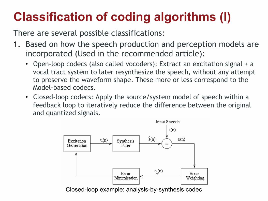
Classification of coding algorithms (I) There are several possible classifications: 1.  Based on how the speech production and perception models are

incorporated (Used in the recommended article): •  Open-loop codecs (also called vocoders): Extract an excitation signal + a

vocal tract system to later resynthesize the speech, without any attempt to preserve the waveform shape. These more or less correspond to the Model-based codecs.

•  Closed-loop codecs: Apply the source/system model of speech within a feedback loop to iteratively reduce the difference between the original and quantized signals.

Speech Analysis - Synthesis & Linear Prediction• Splitting the input speech to

be coded into frames• Parameters determined for

Synthesis filter• Excitation determined to the

filter• Encoder transmits

informationrepresenting the filterparametersand the excitation to thedecoder

• at the decoder the givenexcitation is passed throughthe synthesis filter to givethe reconstructed speech

• AbS Codec Structure

Closed-loop example: analysis-by-synthesis codec

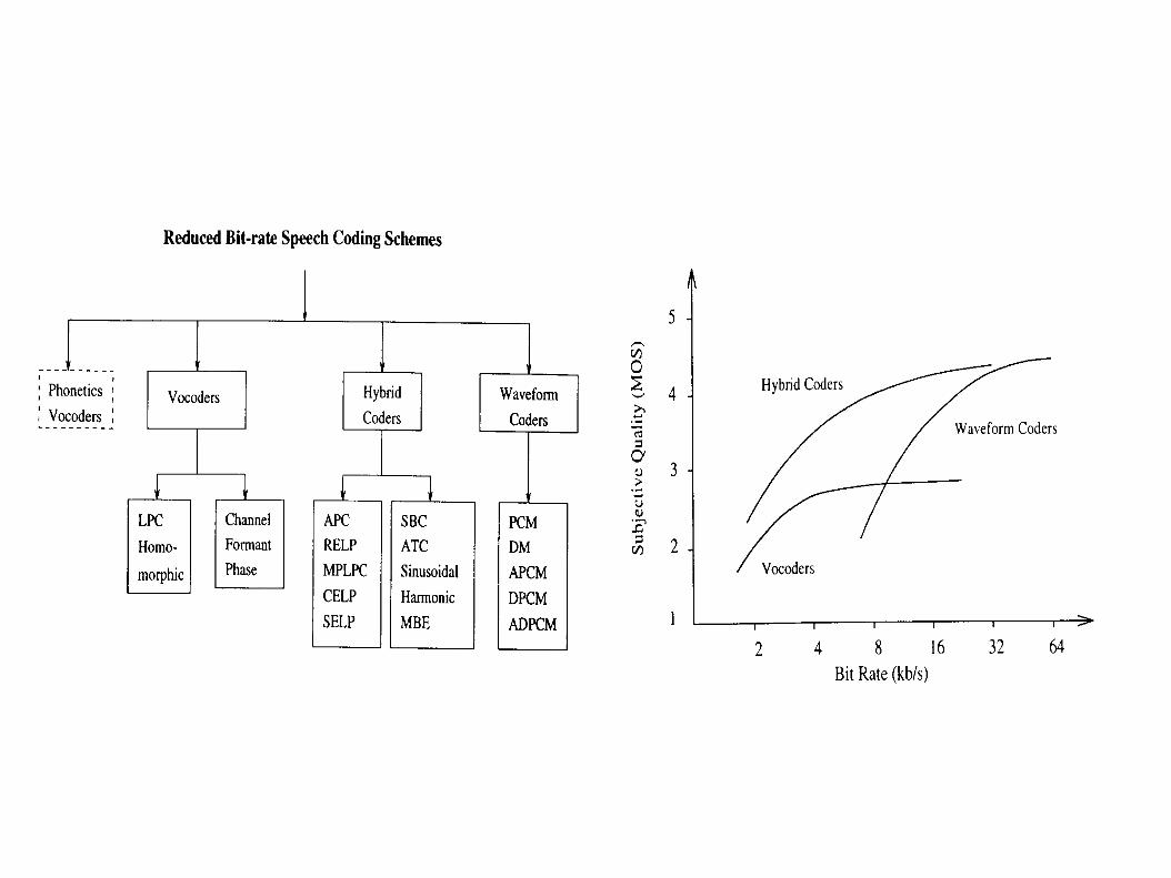
Classification of coding algorithms (II) There are several possible classifications: 2.  Based on how the waveform of the speech signal is preserved

with the process: •  Waveform codecs: aim at reproducing the speech waveform as faithfully as

possible. No previous knowledge is applied to the mechanisms that might have created the audio (for this reason it is not limited to speech). Has higher bit rates but high quality and intelligibility

•  Model-based codecs (also called source-codecs or vocoders): preserve only the spectral properties of speech in the encoded signal. They transmit parameters obtained by modeling speech with a sound production model. Achieves lower bit rates but very synthetic.

•  Hybrid codecs: bring the best of both (i.e. bring certain waveform matching while using the sound production model). These are also called Analysis by synthesis codecs

Classification of coding algorithms (III) 3.  Based on the nature of the encoded parameters:

•  Time-domain coding: speech samples are directly encoded •  Parametric coding: Acoustic parameters are first derived from the

speech samples. These are usually estimated through linear prediction. •  Transform coding: They also send parameters extracted from the

signal. In this case they exploit the redundancy of the signal in the transform domain (Fourier, sinusoid, etc…)


Index for the remainder of the session   Quantization

  Scalar quantization   Uniform   Non-uniform

  Vector quantization

  Time-domain coding   DPCM   ADPCM

  Parametric coding   LPC   Hybrid coding   MP-LPC, CELP

  Transform coding   Sub-band coders   Sinusoidal coding   MPEG-1 layer 3

Quantization

•  Quantization algorithms are at the core of any bigger coding algorithms. They are a clear example of waveform coding techniques, although used in isolation are not very good

•  Scalar quantizers classify each speech sample into one of several levels, represented by B bits

•  Vector quantizers classify several speech samples together into one of several clusters/codebook vectors, each one also represented by a B bits code


Scalar Quantization: Uniform Quantization The decision and reconstruction levels are uniformly spaced. Uniform Pulse-Code Modulation (PCM): Quantizes amplitudes by rounding off each samples to one of a set of discrete values. It is the simplest waveform coding algorithm we will see It is only optimum for signals with a uniform PDF along the peak-to-peak range 2Xm

3-bit quantizer

7.1 Sampling and Quantization of Speech (PCM) 97

Fig. 7.2 8-level mid-tread quantizer.

satisfies the condition

!!/2 < e[n] " !/2, (7.2)

where ! is the quantizer step size. A B-bit quantizer such as the oneshown in Figure 7.2 has 2B levels (1 bit usually signals the sign).Therefore, if the peak-to-peak range is 2Xm, the step size will be! = 2Xm/2B. Because the quantization levels are uniformly spaced by!, such quantizers are called uniform quantizers. Traditionally, repre-sentation of a speech signal by binary-coded quantized samples is calledpulse-code modulation (or just PCM) because binary numbers can berepresented for transmission as on/o" pulse amplitude modulation.

The block marked “encoder” in Figure 7.1 represents the assigningof a binary code word to each quantization level. These code words rep-resent the quantized signal amplitudes, and generally, as in Figure 7.2,these code words are chosen to correspond to some convenient binarynumber system such that arithmetic can be done on the code words as

Sources of error in quantization We can derive 2 sources of error: •  Errors within the dynamic range (see next slide) •  Errors above the dynamic range

•  They are correlated with the signal and need to be avoided by defining well the peak-to-peak range

Sources of error in quantization (II) For samples within the range of the quantizer, the error/noise is

defined as Which has to satisfy Where, if 2Xm is the peak-to-peak range of the signal (no clipping

occurs) and B the number of bits of the quantizer:

We can approximate the SNR of the quantizer as Where σx is the RMS power of the input signal. We therefore gain

6dB for each extra bit we use

e[n]= x[n]! x[n]

!"2< e[n]< "

2

! =2Xm

2B

SNRQ = 6.02B+ 4, 78! 20 log10Xm

! x

"

#$

%

&'


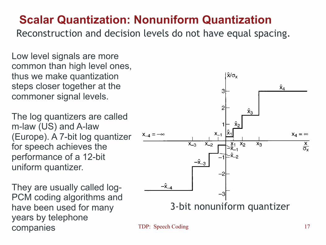
Scalar Quantization: Nonuniform Quantization Reconstruction and decision levels do not have equal spacing.

3-bit nonuniform quantizer

Low level signals are more common than high level ones, thus we make quantization steps closer together at the commoner signal levels. The log quantizers are called m-law (US) and A-law (Europe). A 7-bit log quantizer for speech achieves the performance of a 12-bit uniform quantizer. They are usually called log-PCM coding algorithms and have been used for many years by telephone companies

Non-uniform quantization µ - law

A - law

•  Usually A=87.7, and µ=255 in the standards, and implemented as filters + uniform quantizer. •  The transformation has the effect of distributing samples linearly in the lower levels and

logarithmically in the higher levels

19

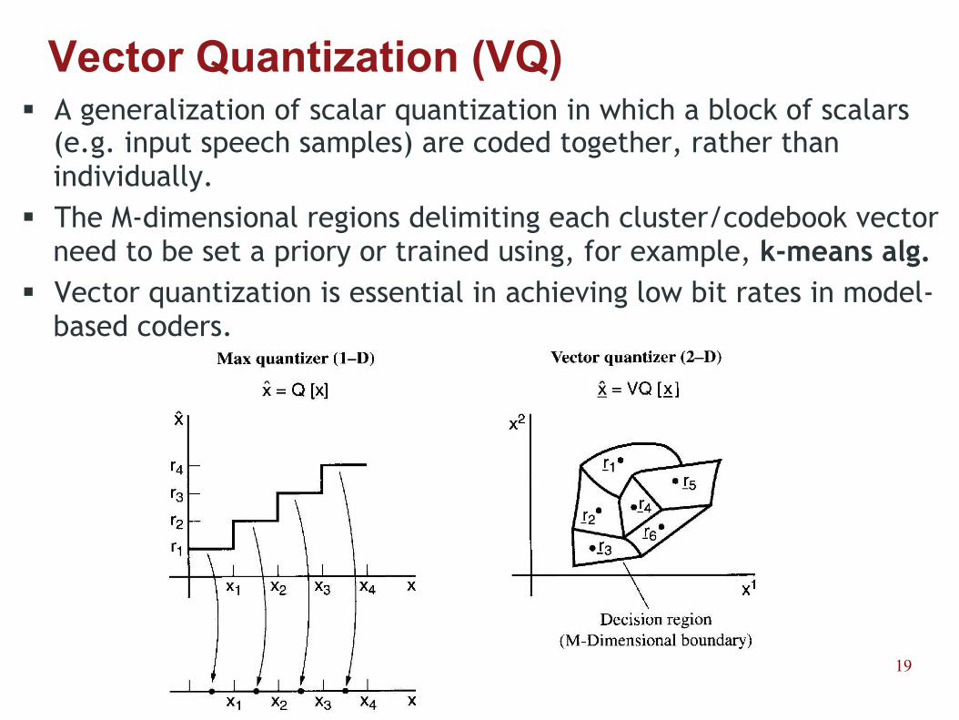
Vector Quantization (VQ)   A generalization of scalar quantization in which a block of scalars

(e.g. input speech samples) are coded together, rather than individually.

  The M-dimensional regions delimiting each cluster/codebook vector need to be set a priory or trained using, for example, k-means alg.

  Vector quantization is essential in achieving low bit rates in model-based coders.


K-Means Clustering 1) Place K points into the space represented by the objects that

are being clustered. These points represent initial group centroids.

2) Assign each object to the group that has the closest centroid. 3) When all objects have been assigned, recalculate the positions

of the K centroids. 4) Repeat Steps 2 and 3 until the centroids no longer move. This

produces a separation of the objects into groups from which the metric to be minimized can be calculated.

K-means clustering

Lineal predictive coding Using the LPC theory we saw earlier, we can estimate the current

speech value from the previous “p” values We can then take the the difference between the real value

(known) and the estimate: If the prediction is good (Gp>1) by quantizing d[n] we can reduce

the quantization error This leads us to a family of methods that use differential coding

that are usually called differential PCM (DPCM)

106 Digital Speech Coding

These coders, which we designate as open-loop coders, are also calledvocoders (voice coder) since they are based on the principles estab-lished by H. Dudley early in the history of speech processing research[30]. A second class of coders employs the source/system model forspeech production inside a feedback loop, and thus are called closed-loop coders. These compare the quantized output to the original inputand attempt to minimize the di!erence between the two in some pre-scribed sense. Di!erential PCM systems are simple examples of thisclass, but increased availability of computational power has made itpossible to implement much more sophisticated closed-loop systemscalled analysis-by-synthesis coders. Closed loop systems, since theyexplicitly attempt to minimize a time-domain distortion measure, oftendo a good job of preserving the speech waveform while employing manyof the same techniques used in open-loop systems.

7.3 Closed-Loop Coders

7.3.1 Predictive Coding

The essential features of predictive coding of speech were set forth in aclassic paper by Atal and Schroeder [5], although the basic principles ofpredictive quantization were introduced by Cutler [26]. Figure 7.5 showsa general block diagram of a large class of speech coding systems thatare called adaptive di!erential PCM (ADPCM) systems. These systemsare generally classified as waveform coders, but we prefer to emphasizethat they are closed-loop, model-based systems that also preserve thewaveform. The reader should ignore initially the blocks concerned withadaptation and all the dotted control lines and focus instead on the coreDPCM system, which is comprised of a feedback structure that includesthe blocks labeled Q and P . The quantizer Q can have a number oflevels ranging from 2 to much higher, it can be uniform or non-uniform,and it can be adaptive or not, but irrespective of the type of quantizer,the quantized output can be expressed as d[n] = d[n] + e[n], where e[n]is the quantization error. The block labeled P is a linear predictor, so

x[n] =p!

k=1

!kx[n ! k], (7.6)

time

d[n]= x[n]! !x[n]

SNR =Gp !SNRq

?

In the coder we eliminate the predictable information from the signal, which is later reincorporated in the decoder. Given that the speech signal changes its characteristics over time, the predictor parameters will need to be recomputed and therefore sent together with the residual.


Time-Domain Coding: Delta Modulation (DM)

•  It is the simplest of the DPCM codecs •  It normally uses only 1-bit quantizer and a first-order predictor •  It is VERY simple to implement and VERY computationally

efficient •  For it to achieve good SNR we need a high bit rate (over the

nyquist frequency) •  Only the quantized output needs to be sent

coder

decoder

25

Time-Domain Coding: Delta Modulation (DM)

When the coding freq. is lot high enough we might not be able to follow the signal

•  We can get lots of error when: •  The signal moves fast and our Δ is too small •  The signal moves slowly and our Δ is too big

26

Time-domain Coding: Adaptive differential PCM •  We can improve DM by automatically adjusting the step size

according to the signal level: •  When there are big changes on the signal we decrease the step size •  When changes are small we increase the step size

•  In general, this corresponds to the systems called Adaptive Differential PCM (ADPCM), which fall within the waveform codecs type

•  ADPCM usually operates on short blocks of input samples, therefore introducing some delay.

•  We can classify the ADPCM systems between feed-forward and feed-backwards (most used)

•  Both the prediction residual and the predictor parameters need to be quantized before sending them •  VQ or non-uniform quantization are the most common techniques

•  The best ADPCM codecs can go as low as 10kbps with acceptable quality

ADPCM systems •  Feed-forward ADPCM

•  Feed-backwards ADPCM

w

w

Model-based/Parametric codecs •  These codecs usually take into account the source-filter model

of speech production to encode speech with acceptable quality at lower bit rates than ADPCM

•  They are usually referred to as VOCODERS. They are open-loop codecs, as they do not have a feedback loop.

•  When they use a speech production model, these algorithms are very good for speech, but create distortions and lack of quality when encoding other signals (e.g. music)

•  By sending only the source/excitation type and the filter parameters, vocoders can achieve very low bitrates

•  With respect to the estimation of the vocal tract parameters, we can classify the vocoders into: •  Homomorphic: Cepstral parameters are extracted and encoded •  LPC: Lineal predictive analysis is used to obtain vocal tract parameters


Parametric Coding: VQ LPC Coder

Hybrid/analysis by synthesis systems •  These systems incorporate some speech-production model (like the

source-filter model) to obtain optimum parameters, that are then sent together with a synthetic excitation signal.

•  Such excitation needs to be efficient to code and produce high quality output speech.

•  In these the signal is also processed in blocks, creating some delay. •  They are called analysis-by-synthesis because a synthetic vocal

tract filter is built iteratively to match the input speech for every given block. Also the excitation is generated from a fixed collection of input components 118 Digital Speech Coding

PerceptualWeighting

W(z)

ExcitationGenerator

Vocal TractFilterH(z)

+][nx ][nd ][ˆ nd

][ˆ nx

-

+ ][nd!

Fig. 7.8 Structure of analysis-by-synthesis speech coders.

perceptual weighting filter, W (z). As the first step in coding a block ofspeech samples, both the vocal tract filter and the perceptual weightingfilter are derived from a linear predictive analysis of the block. Then,the excitation signal is determined from the perceptually weighted dif-ference signal d![n] by an algorithm represented by the block labeled“Excitation Generator.”

Note the similarity of Figure 7.8 to the core ADPCM diagram ofFigure 7.5. The perceptual weighting and excitation generator insidethe dotted box play the role played by the quantizer in ADPCM, wherean adaptive quantization algorithm operates on d[n] to produce a quan-tized di!erence signal d[n], which is the input to the vocal tract system.In ADPCM, the vocal tract model is in the same position in the closed-loop system, but instead of the synthetic output x[n], a signal x[n]predicted from x[n] is subtracted from the input to form the di!erencesignal. This is a key di!erence. In ADPCM, the synthetic output di!ersfrom the input x[n] by the quantization error. In analysis-by-synthesis,x[n] = x[n] ! d[n], i.e., the reconstruction error is !d[n], and a percep-tually weighted version of that error is minimized in the mean-squaredsense by the selection of the excitation d[n].

7.3.4.2 Perceptual Weighting of the Di!erence Signal

Since !d[n] is the error in the reconstructed signal, it is desirable toshape its spectrum to take advantage of perceptual masking e!ects. InADPCM, this is accomplished by quantization noise feedback or preem-phasis/deemphasis filtering. In analysis-by-synthesis coding, the input

Equivalent to the quantizer in ADPCM

Perceptual weighting filter •  The quantization error does not affect all frequencies in the

same way •  In analysis-by-synthesis systems a perceptual weighting filter

changes the frequency shape of the filter residual to modify such error.

•  It is equivalent to the preemphasis filtering in ADPCM •  The perceptual weighting filter W() is designed by inverting the

vocal tract filter H()

7.3 Closed-Loop Coders 119

to the vocal tract filter is determined so as to minimize the perceptually-weighted error d![n]. The weighting is implemented by linear filtering,i.e., d![n] = d[n] ! w[n] with the weighting filter usually defined in termsof the vocal tract filter as the linear system with system function

W (z) =A(z/!1)A(z/!2)

=H(z/!2)H(z/!1)

. (7.14)

The poles of W (z) lie at the same angle but at !2 times the radii ofthe poles of H(z), and the zeros of W (z) are at the same angles but atradii of !1 times the radii of the poles of H(z). If !1 > !2 the frequencyresponse is like a “controlled” inverse filter for H(z), which is the shapedesired. Figure 7.9 shows the frequency response of such a filter, wheretypical values of !1 = 0.9 and !2 = 0.4 are used in (7.14). Clearly, thisfilter tends to emphasize the high frequencies (where the vocal tractfilter gain is low) and it deemphasizes the low frequencies in the errorsignal. Thus, it follows that the error will be distributed in frequency sothat relatively more error occurs at low frequencies, where, in this case,such errors would be masked by the high amplitude low frequencies.By varying !1 and !2 in (7.14) the relative distribution of error can beadjusted.

0 1000 2000 3000 4000!30

!20

!10

0

10

20

30

frequency in Hz,

log

mag

nitu

dein

dB

Fig. 7.9 Comparison of frequency responses of vocal tract filter and perceptual weightingfilter in analysis-by-synthesis coding.

Excitation signal •  A finite set of signals fγk (known at source and destination) can

be used to generate the signal as

•  The selection of the optimum signals and βk is found to optimize the error

•  The excitation signals are defined differently in each algorithm


7.3.4.3 Generating the Excitation Signal

Most analysis-by-synthesis systems generate the excitation from a finitefixed collection of input components, which we designate here as f! [n]for 0 ! n ! L " 1, where L is the excitation frame length and ! rangesover the finite set of components. The input is composed of a finite sumof scaled components selected from the given collection, i.e.,

d[n] =N!

k=1

"kf!k [n]. (7.15)

The "ks and the sequences f!k [n] are chosen to minimize

E =L!1!

n=0

((x[n] " h[n] # d[n]) # w[n])2, (7.16)

where h[n] is the vocal tract impulse response and w[n] is the impulseresponse of the perceptual weighting filter with system function (7.14).Since the component sequences are assumed to be known at both thecoder and decoder, the "s and !s are all that is needed to represent theinput d[n]. It is very di!cult to solve simultaneously for the optimum "sand !s that minimize (7.16). However, satisfactory results are obtainedby solving for the component signals one at a time.

Starting with the assumption that the excitation signal is zero dur-ing the current excitation15 analysis frame (indexed 0 ! n ! L " 1), theoutput in the current frame due to the excitation determined for previ-ous frames is computed and denoted x0[n] for 0 ! n ! L " 1. Normallythis would be a decaying signal that could be truncated after L samples.The error signal in the current frame at this initial stage of the iterativeprocess would be d0[n] = x[n] " x0[n], and the perceptually weightederror would be d"

0[n] = d0[n] # w[n]. Now at the first iteration stage,assume that we have determined which of the collection of input com-ponents f!1 [n] will reduce the weighted mean-squared error the mostand we have also determined the required gain "1. By superposition,x1[n] = x0[n] + "1f!1 [n] # h[n]. The weighted error at the first itera-tion is d"

1[n] = (d0[n] " "1f!1 [n] # h[n] # w[n]), or if we define the per-ceptually weighted vocal tract impulse response as h"[n] = h[n] # w[n]

15 Several analysis frames are usually included in one linear predictive analysis frame.


7.3.4.3 Generating the Excitation Signal

Most analysis-by-synthesis systems generate the excitation from a finitefixed collection of input components, which we designate here as f! [n]for 0 ! n ! L " 1, where L is the excitation frame length and ! rangesover the finite set of components. The input is composed of a finite sumof scaled components selected from the given collection, i.e.,

d[n] =N!

k=1

"kf!k [n]. (7.15)

The "ks and the sequences f!k [n] are chosen to minimize

E =L!1!

n=0

((x[n] " h[n] # d[n]) # w[n])2, (7.16)

where h[n] is the vocal tract impulse response and w[n] is the impulseresponse of the perceptual weighting filter with system function (7.14).Since the component sequences are assumed to be known at both thecoder and decoder, the "s and !s are all that is needed to represent theinput d[n]. It is very di!cult to solve simultaneously for the optimum "sand !s that minimize (7.16). However, satisfactory results are obtainedby solving for the component signals one at a time.

Starting with the assumption that the excitation signal is zero dur-ing the current excitation15 analysis frame (indexed 0 ! n ! L " 1), theoutput in the current frame due to the excitation determined for previ-ous frames is computed and denoted x0[n] for 0 ! n ! L " 1. Normallythis would be a decaying signal that could be truncated after L samples.The error signal in the current frame at this initial stage of the iterativeprocess would be d0[n] = x[n] " x0[n], and the perceptually weightederror would be d"

0[n] = d0[n] # w[n]. Now at the first iteration stage,assume that we have determined which of the collection of input com-ponents f!1 [n] will reduce the weighted mean-squared error the mostand we have also determined the required gain "1. By superposition,x1[n] = x0[n] + "1f!1 [n] # h[n]. The weighted error at the first itera-tion is d"

1[n] = (d0[n] " "1f!1 [n] # h[n] # w[n]), or if we define the per-ceptually weighted vocal tract impulse response as h"[n] = h[n] # w[n]

15 Several analysis frames are usually included in one linear predictive analysis frame.

Where N is the number of signals used to generate the impulse

Where L is the number of samples per block


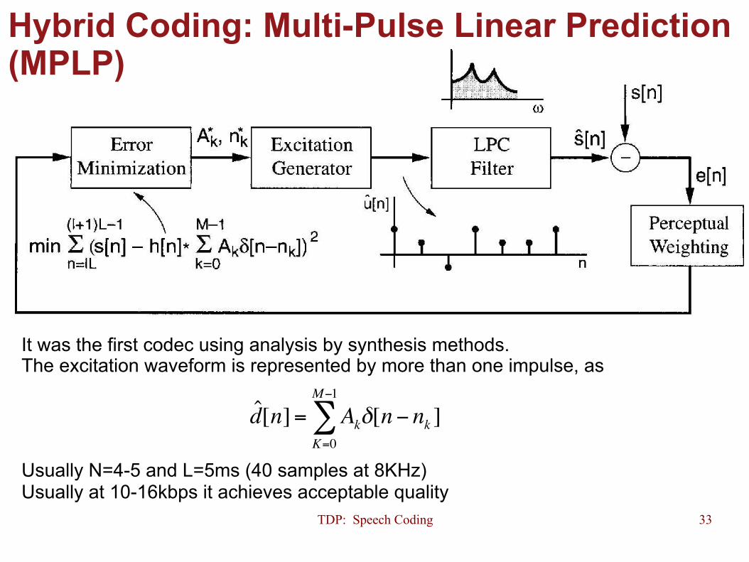
Hybrid Coding: Multi-Pulse Linear Prediction (MPLP)

It was the first codec using analysis by synthesis methods. The excitation waveform is represented by more than one impulse, as Usually N=4-5 and L=5ms (40 samples at 8KHz) Usually at 10-16kbps it achieves acceptable quality

d[n]= Ak!K=0

M!1

" [n! nk ]


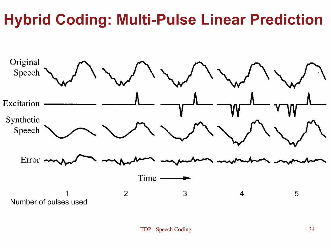
Hybrid Coding: Multi-Pulse Linear Prediction

1 2 3 4 5 Number of pulses used


Code-Excited Linear Prediction (CELP)

  Represents the excitation (residual) from the linear prediction on each frame by codewords from a VQ-generated codebook, rather than multipulse.

  Usually 256-1024 sized codebooks (8-10 bits) are used   On each frame a codeword is chosen from a codebook of

residuals such as to minimize the mean-squared error between the synthesized and original speech waveforms.

  A codebook can be formed by applying a k-means clustering algorithm to a large set of residuals training vectors.

  CELP can achieve acceptable quality at 4,8kpbs   As the search for the optimum sequence is exhaustive it is very

computationally intensive.


Quality versus data rate of coders

Transform-based coding

•  These codecs apply a transformation of the signal to the frequency domain and encode the different bands independently.

•  It takes advantage of the fact that different frequencies have different perception characteristics by human in order to reduce bitrate


Transform Coding: Sub-Band Coders Sub-band and transform coders exploit the redundancy of the

signal in the transform domain.

AT&T sub-band coder and decoder


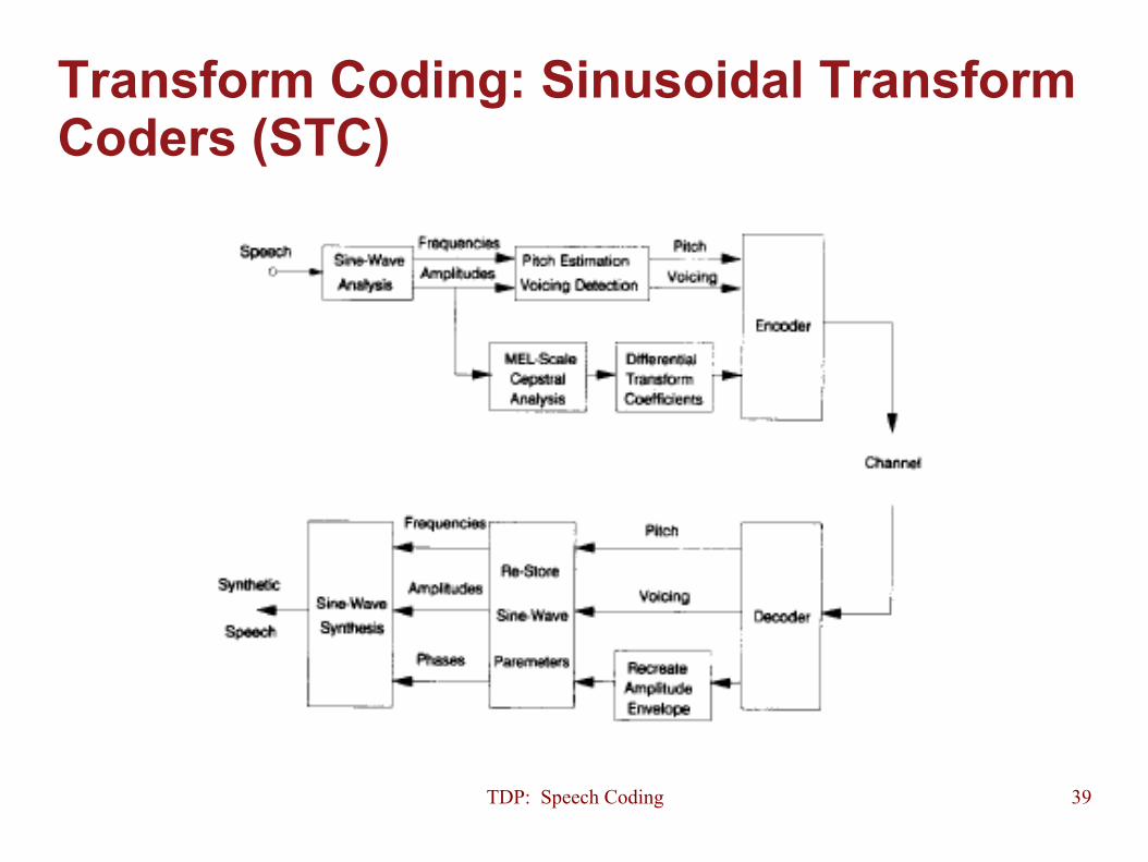
Transform Coding: Sinusoidal Transform Coders (STC)


Transform Coding: MPEG-1

Also known as MPEG2 audio layer 3, or MP3 A transparently lossy audio compression system based on the weaknesses of

the human ear. Can provide compression by a factor of 6 and retain sound quality. Cuantification and coding is done every 8ms

MPEG-1 Audio Features

  PCM sampling rate of 32, 44.1, or 48 kHz   Four modes:

  Monophonic and Dual-monophonic   Stereo and Joint-stereo

  Three modes (layers in MPEG-I speak):   Layer I: Computationally cheapest, bit rates 384Kbps in stereo

(used in DCC)   Layer II: Bit rate ~ 192 kbps in stereo (used in VCD)   Layer III: Most complicated encoding/decoding, bit rates ~ 128kbps

in stereo, originally intended for streaming audio (mp3)

Filter-bank processing •  The FFT is computed every 512/1024 samples (delay of

5.33/10.66ms @48KHz) •  32 bands are then obtained uniformly spaced every 750Hz •  A polyphase filterbank is used: efficient and low delay

Derived filterbank structure that incorpolates the DFT block

21

Data input

Input data for the subband filterbank

31

•  In MPEG-1 layer I blocks of 512 samples are used in the analysis, shifting them 32 samples per step.

•  The encoded output packets cover 12 consecutive shifts/blocks

MPEG 1: Psychoacoustic Model   We Use a psycoacoustic model to determine which frequencies I need

to allocate more bits to   We first use a Hanning weighting window on the signal block, and then

a DFT to convert to frequency domain   The block size is either 512 (layer I) or 1024 (layer II and III) samples.   Example:

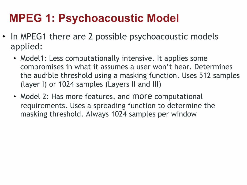
MPEG 1: Psychoacoustic Model •  In MPEG1 there are 2 possible psychoacoustic models

applied: •  Model1: Less computationally intensive. It applies some

compromises in what it assumes a user won’t hear. Determines the audible threshold using a masking function. Uses 512 samples (layer I) or 1024 samples (Layers II and III)

•  Model 2: Has more features, and more computational requirements. Uses a spreading function to determine the masking threshold. Always 1024 samples per window

In the FFT, among other processing, a critical band masking threshold is computed for each critical band frequency

The total masking due to the critical bands is the sum of all

contributions

MPEG 1: Psychoacoustic Model

Prototype spreading functions at z=10 as a function of masker level

59

MPEG 1: Psychoacoustic Model In addition, the minimum auditory threshold is considered to obtain a

total masking threshold

Anything below that threshold is not heart, therefore, does not harm our perceived quality

We calculate a masking threshold for each subband in the polyphase filter bank.

MPEG 1: Psychoacoustic Model In order to use the total masking threshold we compute the signal-to-

mask ratio (SMR) per each of the 32 subbands

SMR = signal energy / masking threshold

Those bands with negative SMR can be encoded with less bits as the generated noise will not affect our perceived quality

MPEG 1: Psychoacoustic Model

What we actually send:

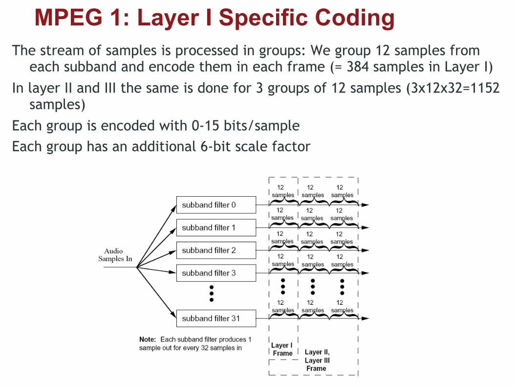
MPEG 1: Layer I Specific Coding The stream of samples is processed in groups: We group 12 samples from

each subband and encode them in each frame (= 384 samples in Layer I) In layer II and III the same is done for 3 groups of 12 samples (3x12x32=1152

samples) Each group is encoded with 0-15 bits/sample Each group has an additional 6-bit scale factor

Documents

7. Speech Coding - Xavier Anguera · What is speech coding? ... • Robustness to transmission errors (e.g. intermittent cuts in ... • A minimum of 30 people has to grade speech