Embed Size (px)
Citation preview
A Quality Assurance Project Plan for Monitoring Gaseous and Particulate Matter Emissions from Broiler Housing Section No.: 7
Version 1.3 09/13/06
Page 1 of 14
7.0 Quality Objectives and Criteria for Measurement Data 7.1 Data Quality Objectives (DQOs) Background The overall objective of this data acquisition project is to generate data of sufficient quality to satisfy the research objectives of the previously stated project. Data will undergo quality assurance review, which among other things will assess data representativeness, data completeness, comparability, and accuracy (USEPA document QA/G-5). The intended use of the collected data is to provide an estimation of daily emissions of gases and particulates (emissions of NH3, TSP, PM10, PM2.5, H2S and NMHC) from commercial broiler production houses in the southeastern United States. The collected data will provide insight into temporal variability (such as bird age, seasonal effects, and other temporal effects) and spatial variability (two houses on two separate sites are monitored). This variability has been previously estimated in earlier studies in Kentucky and Pennsylvania broiler houses (Wheeler et al., 2006) and bird age was found to be the predominant factor in variation over time. Variation between houses (eight houses on two sites in Kentucky, and four houses on two sites in Pennsylvania) was found to be relatively small when other factors were held constant (e.g., bird age). Data Quality Data representativeness is ensured by the overall sampling design, which includes high frequency (on order of several times per hour) sampling over a 12-month measurement period at two similar broiler operations at different locations in western Kentucky. This is described in detail in Section 11: Sampling Process Design. Underlying theoretical considerations that impact the representativeness of data by direct or component determination are outlined in this section. “Data completeness is a measure of the amount of valid data obtained from a measurement system, expressed as a percentage of the number of valid measurements that should have been collected” (USEPA. 2002. EPA Guidance for Quality Assurance Project Plans. EPA QA/G-5). In this study, data completeness is achieved by ensuring that valid building emission data obtained from the measurement system is no less than 75% of the scheduled sampling. A greater percentage does not seem reasonable with potential lightning strikes, equipment breakdowns, university and broiler integrator schedules, and farm related problems. Using total daily emissions as the primary Data Quality Objectives (DQOs), we thus require a minimum of eighteen hours of sampling for daily emission to be used. Data completeness is ensured by 1) using properly maintained and reliable instrumentation, 2) maintaining a ready supply of spare parts, 3) installing electrical backups such as uninterruptible power supplies, 4) regular on-site calibration checks and inspections, 5) frequent remote access to the DAQ computer, and 6) local broiler production management collaboration and cooperation.
28

A Quality Assurance Project Plan for Monitoring Gaseous and Particulate Matter Emissions from Broiler Housing Section No.: 7
Version 1.3 09/13/06
Page 2 of 14 Data comparability is maintained by 1) employing equivalent analytical methods (where appropriate and available methods exist) and a sampling protocol used in recent emission studies in confined livestock and poultry facilities, 2) continuous, automatic collection of bird live body mass so that emission rates can be expressed on either per bird basis or per animal unit (500 kg live body mass), 3) comparison of measurements with previous mass balance and emissions rate measurements reported for poultry buildings, and 4) through the use of common equipment and protocols at both sites. Development of DQOs Accuracy is a two-part quality indicator and includes both bias (systematic error) and precision (random error). Accuracy is a measure of the closeness of an individual measurement or the average of a number of measurements to the true value (EPA QA/G5). Accuracy of the measured value will be expressed in terms of percentage below or above the known value and in terms of the absolute difference between the measured value and the known value. Precision is a measure of agreement among replicate measurements of the same property, under prescribed similar conditions (EPA QA/G5). Precision is defined as the standard deviation of replicate measurements of the concentration of a known pollutant expressed as a percentage difference from the known value. Concentration measurement accuracy (bias and precision) is maintained by regular calibration of the instruments, which involves challenging the measurement system to perform replicate analyses of the samples with known concentrations. Ventilation rate measurement accuracy is maintained by regular testing of all the ventilation fans at the start and at the end of the study and a subset of the fans after each flock production. If the subset of fans is found to exceed the predetermined uncertainty tolerance (i.e., 10% deviation from the previous value), all fans will be recalibrated before the next flock. In all cases, a clear schedule of calibration is documented and adhered to. In addition, all the fans will be thoroughly cleaned and conditions of the belts checked before the onset of each flock. Static Calibration is a formalized methodology for removing measurement bias and quantifying measurement precision (Doeblin, 1990). A static calibration in which measurements are regressed against “true” or standard values with equivalent units allows for direct quantification of precision from the standard error of the regression and a hypothesis test regarding whether bias exists (e.g., non-unity slope). If bias exists, it is removed by inversion of the calibration regression, and the standard error of regression is adjusted by dividing by the (non-unity) slope of regression. This standard error(s) can then be utilized to make meaningful statistical bounds on the uncertainty of a measurement post-calibration. For example, by the use of 2-second limits and assuming normally distributed random errors, the point estimate from the instrument is within 2-second limits or ±2.5% of the “true” value. This also assumes that the value(s) for the standard used in the calibration is of much greater absolute accuracy, somewhat problematic for example with calibration gases that are at best 2-3% of stated value. For example, the FANS system used to calibrate individual ventilation fans has been demonstrated to exhibit an imprecision of 139 m3 h-1 (83 cubic feet per minute (cfm)) (Gates et al., 2004) as represented by the (adjusted) standard error of regression for 10 FANS units calibrated at the University of Illinois BioEnvironmental and Structural Systems (BESS)
29
A Quality Assurance Project Plan for Monitoring Gaseous and Particulate Matter Emissions from Broiler Housing Section No.: 7
Version 1.3 09/13/06
Page 3 of 14 Laboratory. Three sigma (3s) limits (which comprise 99.7% of the expected error) on the precision of fan ventilation rate are thus on the order of 417 m3 h-1 (249 cfm), remarkably accurate for fans that nominally run at 17,000 to 34,000 m3 h-1 (10,000 to 20,000 cfm). To state the FANS accuracy in terms of precision as is defined in EPA QA/G5 requires knowledge of the actual flow rate since accuracy is expressed on a percentage basis. For example, the 417 m3 h-1 accuracy translates to a 2.4% error for a single 36-inch sidewall fan at a nominal flow rate of 17,000 m3 h-1; but 1.2% error for a 48-inch tunnel fan with a nominal flow rate of 34,000 m3 h-1. Consequently, while it may be considered convenient to express the DQOs in terms of percent imprecision, it is important to recognize that small absolute errors in measurement may be expressed as large relative errors on a percentage basis. For example, the same 3s limit applied to a 1,700 m3 h-1 flow rate yields an “imprecision” of 24% using the G5 definition (see Gates et al., 2004, for additional analysis and discussion). A similar statement may be made for each of the concentration measurements in this study. Because of the continuous nature of our concentration measurements, static calibration is critical, and especially important to remove bias and to reduce the measurement uncertainty to that of the instruments’ effective random errors. This can be understood by considering the cumulative effect that a biased concentration reading would have on estimation of daily ER. For example, assuming constant concentration and constant ventilation rate over a 24-h period, and assuming a 10% positive bias in the concentration reading, we would then see a 10% over-prediction of ER for the 24-h period. If instead the measurement error in concentration was 10% of reading, but it was completely random and centered about zero, then we would expect an error in ER of ±5% or less. Dynamic response of instruments is important to determine an appropriate sampling frequency for locations within a site. In this study, a single instrument is used to sample gas concentrations from two to four locations on a site (one outside measurement for background and up to three locations within each broiler house). Each instrument may exhibit different transient response characteristics when multiplexed across multiple locations, and to measure different gases. A sufficient number of samples at one location must be taken to ensure that the instrument’s settling time is exceeded. Settling time is defined as the time required by an instrument to achieve and remain within a specified tolerance band around the assumed constant final value. For example, a 5% settling time means the time required for an instrument to achieve and remain within 95 to 105% of the final value. Our research suggests that the critical gas measurement (with maximum settling time) in this study is ammonia. Figure 7.1 illustrates that a 4% settling time equates to nearly 2 minutes (Moody et al., 2006). Thus, to ensure that an accurate sample is acquired, repeated sampling at a location should occur for 120 seconds before multiplexing to another location.
30

A Quality Assurance Project Plan for Monitoring Gaseous and Particulate Matter Emissions from Broiler Housing Section No.: 7
Version 1.3 09/13/06
Page 4 of 14
0
44
75
87
100100100100999694
9997
0
20
40
60
80
100
0:00 0:30 1:00 1:30 2:00 2:30 3:00 3:30 4:00 4:30 5:00
Time, min:sec
0
5
10
15
20
25
Percentage of Span Gas, % NH3 Concentration, ppm
Figure 7.1. INNOVA analyzer dynamic response to step change in ammonia. The settling time is
approximately 120 seconds to better than 96% of true span (100% = 22.8 ppm). The dynamic response characteristic exhibited in Figure 7.1 is typical of a first order measurement system (Doeblin, 1990). For first order instruments, a 5% settling time corresponds to 2 time-constants (2τ), which indicates that the time constant for the Innova 1412 is about 52.5 seconds (2τ = 105 seconds) when measuring ammonia. Component Error Analysis Component Error Analysis is used to quantify uncertainty when a quantity such as daily emission rate is calculated from multiple measurements, each with its own degree of accuracy. A component error analysis (Doeblin, 1990) provides statistical meaning to a statement on the magnitude of error in the calculation of daily emission rate. This analysis has been performed for an earlier project that measured broiler house ammonia emissions and was documented in a copyrighted Ph.D. dissertation (Casey, 2005). A manuscript (in preparation) on this topic, for broiler house ammonia emissions, was used in the following description (Casey et al., 2007). Daily ER is computed as the sum of multiple ER values obtained from measurements over the course of the day, with each ER computed from the product of ventilation rate and concentration difference. The ventilation rate must be converted to standard conditions so that interior and outside temperatures and barometric pressure must also be measured. These key measurements affect the uncertainty of daily ER.
31
A Quality Assurance Project Plan for Monitoring Gaseous and Particulate Matter Emissions from Broiler Housing Section No.: 7
Version 1.3 09/13/06
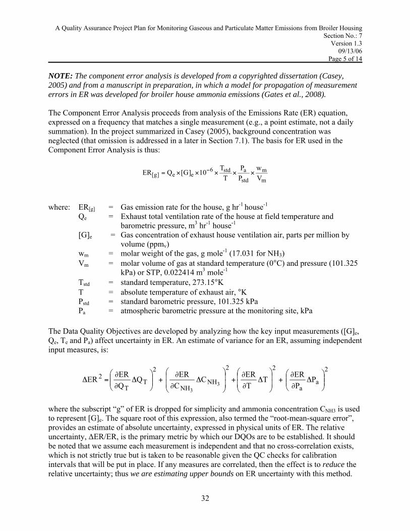
Page 5 of 14 NOTE: The component error analysis is developed from a copyrighted dissertation (Casey, 2005) and from a manuscript in preparation, in which a model for propagation of measurement errors in ER was developed for broiler house ammonia emissions (Gates et al., 2008). The Component Error Analysis proceeds from analysis of the Emissions Rate (ER) equation, expressed on a frequency that matches a single measurement (e.g., a point estimate, not a daily summation). In the project summarized in Casey (2005), background concentration was neglected (that omission is addressed in a later in Section 7.1). The basis for ER used in the Component Error Analysis is thus:
m
m
std
astd6ee]g[ V
wPP
TT10]G[QER ×××××= −
where: ER[g] = Gas emission rate for the house, g hr-1 house-1 Qe = Exhaust total ventilation rate of the house at field temperature and
barometric pressure, m3 hr-1 house-1 [G]e = Gas concentration of exhaust house ventilation air, parts per million by
volume (ppmv) wm = molar weight of the gas, g mole-1 (17.031 for NH3) Vm = molar volume of gas at standard temperature (0°C) and pressure (101.325
kPa) or STP, 0.022414 m3 mole-1 Tstd = standard temperature, 273.15°K T = absolute temperature of exhaust air, °K
Pstd = standard barometric pressure, 101.325 kPa Pa = atmospheric barometric pressure at the monitoring site, kPa The Data Quality Objectives are developed by analyzing how the key input measurements ([G]e, Qe, Te and Pa) affect uncertainty in ER. An estimate of variance for an ER, assuming independent input measures, is:
2
aa
22
NHNH
2
TT
2 PPERT
TERC
CERQ
QERER
33
⎟⎟⎠
⎞⎜⎜⎝
⎛Δ
∂
∂+⎟
⎟⎠
⎞⎜⎜⎝
⎛Δ
∂
∂+
⎟⎟⎠
⎞⎜⎜⎝
⎛Δ
∂
∂+⎟⎟
⎠
⎞⎜⎜⎝
⎛Δ
∂
∂=Δ
where the subscript “g” of ER is dropped for simplicity and ammonia concentration CNH3 is used to represent [G]e. The square root of this expression, also termed the “root-mean-square error”, provides an estimate of absolute uncertainty, expressed in physical units of ER. The relative uncertainty, ΔER/ER, is the primary metric by which our DQOs are to be established. It should be noted that we assume each measurement is independent and that no cross-correlation exists, which is not strictly true but is taken to be reasonable given the QC checks for calibration intervals that will be put in place. If any measures are correlated, then the effect is to reduce the relative uncertainty; thus we are estimating upper bounds on ER uncertainty with this method.
32

A Quality Assurance Project Plan for Monitoring Gaseous and Particulate Matter Emissions from Broiler Housing Section No.: 7
Version 1.3 09/13/06
Page 6 of 14 In this equation, there are two classes of terms in each product on the right hand side, namely the partial differentials of ER with respect to a primary measurement and the error in that measurement (denoted by Δ). The partial differentials relate the physical relationships between measurements to the computed quantity. Errors in each measurement (Δ-values) are assigned two-standard deviations, as determined from calibration standard errors; this provides a statistically meaningful assessment for uncertainty in terms of a 95% confidence statement (Doeblin, 1990) on the estimated uncertainty. For this analysis, we take the estimated precision listed in Table 7.1 as the basis for the Δ-values in the equation for ΔER. By increasing these to the threshold value that constitutes a required recalibration (typically 5% for most instruments) we can perform a sensitivity analysis and determine which measurements contribute the majority of uncertainty to ΔER. For total building ventilation, the partial differential ∂ER/∂QT in turn relates individual measurements taken by the Fan Assessment Numeration System to construct an individual fan calibration curve in-situ, thus requiring measurements of building static pressure (Pd) and a regression slope (b) and intercept (a) that is unique to each fan in the building. Other partial differentials are more straightforward, relating ER directly to measurements. We present without derivation the following equation in which the partial derivatives have been expanded. This equation forms the basis for the DQOs that have been established.
⎟⎟⎟
⎠
⎞
⎜⎜⎜
⎝
⎛
⎟⎟⎠
⎞⎜⎜⎝
⎛Δ
∂
∂+⎟
⎟⎠
⎞⎜⎜⎝
⎛Δ
∂
∂+⎟
⎟⎠
⎞⎜⎜⎝
⎛Δ
∂
∂
⎟⎟⎠
⎞⎜⎜⎝
⎛
∂
∂⎟⎟⎠
⎞⎜⎜⎝
⎛=Δ
2
dd
j2
jj
j2
jj
j2
j
T2
T
2 PPQ
bbQ
aaQ
QERER
⎟⎟⎟
⎠
⎞
⎜⎜⎜
⎝
⎛
⎟⎟⎠
⎞⎜⎜⎝
⎛Δ+⎟
⎟
⎠
⎞
⎜⎜
⎝
⎛Δ
−+⎟
⎟⎠
⎞⎜⎜⎝
⎛Δ⎟
⎠⎞
⎜⎝⎛+
2
NHSpan
Cal2
span2span
cal2
calSpan
NH2
33 x
CC
CC
CC
C
x
CER
2
aa
2
2P
P
ERTT
ER⎟⎟
⎠
⎞
⎜⎜
⎝
⎛Δ+⎟
⎟
⎠
⎞
⎜⎜
⎝
⎛Δ
−+
Terms in this equation include variables defined previously, plus:
Qj = aj + bj Pd is the relation for an individual fan ventilation rate Ccal = calibration span gas certified value (within 2 - 3%) Cspan = Ccal (derivation was for a system with discrepancy between indicated and
supplied values owing to instrumentation resolution differences that do not exist in the system here)
xNH3 = concentration indicated by instrument To assess ER uncertainty, the above equation is evaluated at representative values. Uncertainties for the primary measurements are given by precision values in Table 7.1. Concentration data for
33

A Quality Assurance Project Plan for Monitoring Gaseous and Particulate Matter Emissions from Broiler Housing Section No.: 7
Version 1.3 09/13/06
Page 7 of 14 the various gas and dust constituents in this study are 1% or better (Table 7.1), with a 5% limit for required recalibration.
Table 7.1. Sampling parameter and equipment quality control objectives.
Parameter Sample Matrix Analyzer Matrix
DetectionLimit
QuantitationLimit
EstimatedPrecision
QC Check
QC limit Action
NH3 Air INNOVA 1412 0.2 ppm 2000 ppm ±1% weekly 5% CalibrateCO2 Air INNOVA 1412 3.4 ppm 34,000 ppm ±1% weekly 5% CalibrateCH4 Air INNOVA 1412 0.4 ppm 4000 ppm ±1% weekly 5% Calibrate
Non-CH4 Air INNOVA 1412 0.02 ppm 200 ppm ±1% weekly 5% CalibrateH2S Air API 101E 0.4 ppb 20000 ppb ±0.5% weekly 5% CalibrateCH4 Air VIG 200 0.1 ppm 100 ±1% weekly 5% Calibrate
Non-CH4 Air VIG 200 0.01 ppm 10 ±1% weekly 5% Calibrate
Temperature Air Type T Thermocouple -40°C 50ºC 0.5ºC Every
flock 0.5°C Calibrate
RH Air HMW 61U 2% 95% 2% Six months 5% Calibrate
S. Pressure Air Setra 264 2 Pa 125 Pa ±1% Six months 5% Calibrate
Barometric pressure Air WE100 0.8 bar 1.1 bar ±1% Six
months 5% Calibrate
TSP Air TEOM 1400 0.01 μg/m3 ±5 μg/m3 Yearly 5% CalibratePM10 Air TEOM 1400 0.01 μg/m3 ±5 μg/m3 Yearly 5% CalibratePM2 5 Air TEOM 1400 0.01 μg/m3 ±5 μg/m3 Yearly 5% Calibrate
Fan flow rate Air 200 m3h-1 Every flock 10% Calibrate
Fan run time Air Current Switch 1.0 Aac 100 Aac Every flock Replace
on failure Other factors that influence DQOs Three factors have been overlooked in the analysis of error propagation presented above. These are effect of multiple fans in building ventilation rate, effect of fan performance degradation during each flock grow-out because of accumulation of dirt on fans, and the effect of neglecting background concentration and differences between inside and outside air density and moisture content. Each factor is briefly addressed below. Effect of Multiple Fans—Variance of an expression that is comprised of a constant multiplied by another varying quantity is given as the constant times the variance of the input quantity. Thus, for 14 ventilation fans with identical uncertainty, the uncertainty in total building ventilation is √14·uncertainty in an individual fan ventilation rate. Effect of Fan Degradation During Grow-Out—As fans accumulate dust and dander, their performance degrades. This degradation has been shown to be significant. Regular cleaning between each flock is performed and confirmed with in-situ recalibration of a random subset of
34

A Quality Assurance Project Plan for Monitoring Gaseous and Particulate Matter Emissions from Broiler Housing Section No.: 7
Version 1.3 09/13/06
Page 8 of 14 fans in each building; however, quantification of degradation is not realistic and thus introduces a bias towards over-estimating ventilation rate, and hence building emission rate. Effect of Background Concentration and Air Density/Moisture Effects on ER—The component error analysis cited (Casey, 2005; Casey et al., 2007) neglected background ammonia concentration. Other studies have incorporated background concentration but have performed a pseudo-mass balance that neglects effects of differing air densities between outside and inside air. This section outlines the error associated with these two omissions. In general, the impact of these omissions on ER for the methods proposed in this study is inconsequential. However, the ER methodology employed in this study properly accounts for both background concentrations and differences in air density. Note that our study corrects for both background concentration and air density difference. This analysis is provided to demonstrate the importance of including both these corrections when quantifying ER. Building emission rate of any substance, ER, is given by:
m
m
std
astd
6
i
i
e
i
e
ee]g[ V
wPP
T10)T
]G[T
]G[(QER ×××××
υ
υ−= −
where: ER[g] = Gas emission rate for the house, g hr-1 house-1 Qe = Exhaust ventilation rate of the house at field temperature and barometric
pressure, m3 hr-1 house-1 [G]i,[G]e = Gas concentration of incoming and exhaust house ventilation air,
respectively, parts per million by volume (ppmv) wm = molar weight of the gas, g mole-1 (17.031 for NH3) Vm = molar volume of gas at standard temperature (0°C) and pressure (101.325
kPa) or STP, 0.022414 m3 mole-1 Tstd = standard temperature, 273.15°K Ti, Te = absolute temperature of incoming and exhaust air, respectively, °K
Pstd = standard barometric pressure, 101.325 kPa Pa = atmospheric barometric pressure at the monitoring site, kPa
νi, νe = specific volume of incoming and exhaust air, respectively, m3 moist air per kg dry air, calculated from air temperature and RH
Specific volume of moist air at (T, Pa) is computed from:
a
daP
)W6078.11(TR +=ν
where: Rda = dry air universal gas constant, 287.055 J kg-1 K-1 W = humidity ratio, kg water vapor kg-1 dry air
35

A Quality Assurance Project Plan for Monitoring Gaseous and Particulate Matter Emissions from Broiler Housing Section No.: 7
Version 1.3 09/13/06
Page 9 of 14 Humidity ratio at a given temperature and relative humidity obtained from:
wa
wPP
P62198.0W
−=
wsw PP φ=
)Tln(CTCTCTCTCCT/C)Pln( 74
63
52
4321ws ++++++= ; –100 < t < 0°C
)Tln(CTCTCTCCT/C)Pln( 133
122
111098ws +++++= ; 0 < t < 200°C where: ø = relative humidity, decimal Pw = water vapor partial pressure, Pa Pws = water vapor saturation pressure, Pa C1, C13 = given e.g. ASHRAE HOF (2005) page 6.2 equations 5 and 6 The specific volume ratio νi/νe, is:
)W1)(W6078.11(T)W1)(W6078.11(T
iee
eii
e
i++
++=
ν
ν
Substitution into the equation for ER gives:
m
m
std
astd
6
ie
eiie
e
e]g[ V
wPPT10
)W1)(W6078.11()W1)(W6078.11(]G[]G[
TQER ××××
⎭⎬⎫
⎩⎨⎧
++
++−= −
The effect on ER[g] of neglecting background concentration [G]I is quantified in Table 7.2 for a broad range in expected indoor and outdoor temperature and humidity ratios. The following points can be made:
1. Neglecting a positive, non-zero background concentration can result in over-predicting ER by 0 to 15%. This is a bias in ER estimation.
2. The specific volume ratio νi/νe provides a multiplier of 103% to 115% to the background concentration, resulting in potential further over-prediction.
3. The greatest over-prediction will occur during the coldest and driest outside conditions coupled with the warmest and most humid interior conditions, and is about 15% for typical Kentucky winter time brooding conditions.
4. Note that the adjustment in the table below is applied to the background gas concentration, not the ER. Thus, the error in ER from neglecting density effects is less than 15% of the background concentration; the error in ER from neglecting background concentration depends on the magnitude of [G]e and [G]i.
36

A Quality Assurance Project Plan for Monitoring Gaseous and Particulate Matter Emissions from Broiler Housing Section No.: 7
Version 1.3 09/13/06
Page 10 of 14
Table 7.2. Temperature and humidity adjustment ratio of air emissions.
Humidity Ratio (kg H20/kg dry air) Air Temperature (K) Adjustment Inlet Exhaust Inlet Exhaust
Comment Wi We Ti Te ratio* Winter brooding 0.000 0.020 263 306 115.0% Winter growout 0.002 0.012 263 293 110.7% Fall/spring brooding 0.004 0.020 273 306 111.0% Fall/spring dry interior 0.004 0.010 273 306 111.7% Fall/spring growout 0.004 0.010 283 293 103.2% Summer brooding 0.010 0.020 293 306 103.8% Summer growout 0.010 0.012 293 293 103.4% * Multiply background (ppm) by “ratio” to get adjustment for air density differences.
37

A Quality Assurance Project Plan for Monitoring Gaseous and Particulate Matter Emissions from Broiler Housing Section No.: 7
Version 1.3 09/13/06
Page 11 of 14 7.2 Measurement Quality Objectives (MQOs) According to EPA QA/G-5, p 27:
“Measurement performance criteria for new data collection efforts are stated in terms of the desired (assumed) level of uncertainty in data that will be used to address the study question or support the decision. When possible, it is desirable to state measurement performance criteria in quantitative terms, such as limits on analytical imprecision, bias and method detection limits, and limits on the overall variance of study results (to include spatial and temporal variability).”
Thus, in the remainder of this section, we utilize the analysis used to develop the DQOs to justify and document our selection of acceptable limits on uncertainty in the emissions data, denoted as ER (Emission Rate), expressed on a mass of constituent emitted from the building in a consecutive 24-hour period normalized to a per-bird basis (e.g. kg of pollutant bird-1 day-1). This unit is selected so that ER from broiler houses with different numbers of birds can be compared and provide information regarding spatial variability in the data. This analysis establishes expectations for MQOs. Representative Calculations to Define Measurement Quality Objectives A previously conducted component error analysis (Casey, 2005) suggests that if 3-second limits on ventilation rate and 1% accuracy on ammonia were maintained then the uncertainty in ER is 2-3%. Relative uncertainty was found to decrease as the number of fans being used increased, and was largely unaffected by ammonia concentration in the building over the range of 10 to 100 ppm. Increasing both ventilation uncertainty (to 10% of reading) and ammonia concentration uncertainty (to 3 ppm) causes substantially greater uncertainty in ER, with a range from 4.9% (8 fans, 100 ppm) to 19% (1 fan, 10 ppm). This prior analysis approach served as the basis for establishing DQOs for this study. However, it is important to utilize the proper instrumentation uncertainties for the equipment selected for this study. The previously cited study utilized less accurate sensors to measure ammonia concentration and so the uncertainties for this study are expected to be improved. For purposes of establishing MQOs for this study, we performed a sensitivity analysis using the component error analysis equations provided in the preceding section coupled with reasonable estimates of uncertainty for the equipment used in this study. This establishes MQOs for a single ER estimation. We investigated two cases: Case 1: 1% uncertainty on concentration measurement, 3% uncertainty on calibration standard,
and a range of 1% to 10% uncertainty in building ventilation rate. Since building ventilation rate is comprised of multiple fans, we assumed them to be identical and the total building ventilation rate uncertainty is the number of fans multiplied by the ventilation rate uncertainty of a fan.
Case 2: Similar to case 1, except that concentration measurement uncertainty is increased to the
threshold for recalibration as per Table 7.1
38

A Quality Assurance Project Plan for Monitoring Gaseous and Particulate Matter Emissions from Broiler Housing Section No.: 7
Version 1.3 09/13/06
Page 12 of 14 Results of these two cases are presented graphically in Figure 7.2 below. Relative uncertainty (%) is plotted against building ventilation rate, and found to follow a power law relation given by:
( )b)cfm(VRa(%)ERER
⋅=Δ
where constants (a,b) are obtained from nonlinear regression and building ventilation rate is given in units of cubic feet per minute (cfm). These constants are tabulated, along with statistical measures of goodness of fit of the power law equation, in Table 7.3.
Table 7.3. Parameters for predicting emission rate (ER) uncertainty as affected by concentration and ventilation uncertainties.
Case
Ventilation Uncertainty
% Adjusted
r2 a (se)
% b (se)
1 0.9999 4.1804 (0.1604) -0.0239 (0.0036) 2.5 0.9994 10.5805 (1.055) -0.1033 (0.0094) 5 0.9986 62.0504 (8.501) -0.2513 (0.0131) 7.5 0.9984 205.951 (29.28) -0.3458 (0.138)
1% Concentration Uncertainty, 3% Calibration Gas
10 0.9993 415.278 (38.64) -0.3939 (0.091) 1 1.0000 6.2003 (0.09877) -0.0045 (0.0015) 2.5 0.9999 8.7914 (0.4232) -0.0353 (0.0045) 5 0.9992 22.432 (2.4846) -0.1156 (0.0104) 7.5 0.9987 60.004 (8.2516) -0.1981 (0.0131) 10 0.9985 142.291 (19.70) -0.2690 (0.0133)
5% Concentration Uncertainty, 3% Calibration Gas
25 0.9997 1509.8 (87.17) -0.4362 (0.0057)
3% Cal Gas, 1% Concentration Uncertainty
VR (cfm)
0 20x103 40x103 60x103 80x103 100x103 120x103
ER U
ncer
tain
ty (%
)
2
4
6
8
10
12
14
10%7.5%5%2.5%1%
Ventilation Uncertainty
3% Cal gas, 5% Concentration Uncertainty
VR (cfm)
0 20x103 40x103 60x103 80x103 100x103 120x103
ER U
ncer
tain
ty (%
)
5
10
15
20
25
30
35
25%10%7.5%5%2.5%1%
Ventilation Uncertainty
Figure 7.2. Uncertainty estimates for ER as function of building emission rate and ventilation
uncertainty.
39

A Quality Assurance Project Plan for Monitoring Gaseous and Particulate Matter Emissions from Broiler Housing Section No.: 7
Version 1.3 09/13/06
Page 13 of 14 In all cases, an excellent fit was obtained, with adjusted r2 > 0.99. This allows estimation of uncertainty in ER for other values of input parameters. While this analysis was carried out specifically for ammonia, it applies equally to all gaseous contaminants being measured in this study, which have stated accuracies of 1% or better. For particulates the analysis also applies, but since the particulate accuracy is represented in terms of an absolute mass concentration (5 ug/m3), it is directly applicable to concentrations greater than 500 ug/m3. For this project, uncertainty in ER estimates can be directly developed from Figure 7.2. The left-hand pane is representative of calibrated concentration-measuring instrumentation (1% uncertainty), with 50% error in calibration gas certification (i.e. 3% uncertainty for a 2% certification). It shows that as ventilation rate increases the uncertainty drops to around 4%. Uncertainty is highest as ventilation rate uncertainty increases, with the maximum value given as about 12% when ventilation uncertainty is 10% at very low ventilation rates. Thus, it is reasonable to expect that individual ER measurement uncertainties can be maintained to fewer than 10% since the minimum ventilation rate of the houses being monitored is approximately 23,000 CFM. The uncertainty estimates in the right-hand plot of Figure 7.2 establish the effect of increasing concentration uncertainty from 1% to 5%, for example, a 5-fold increase in uncertainty, while all else is held constant. For this scenario, overall uncertainty in ER increases by very little. Also added is a severe case in which ventilation rate uncertainty is increased to 25%, for example, if fans were not calibrated but instead measured via hot wire anemometer or some less-sophisticated methodology. For studies using such methods, ER uncertainty can approach 30%. From this component error analysis, it is clear that careful control of ventilation rate uncertainty is critical for controlling ER uncertainty, and has probably contributed to the majority of error in such measurements prior to the implementation of the FANS methodology with regular calibration of individual fans. If ventilation rate is estimated by other, less accurate, methods then ER uncertainty is expected to be substantially larger. This defines a critical MQO for this study. ER uncertainty should be maintained at less than 10% using the instrumentation and QC checks outlined in the DQO section and listed in Table 7.1. Uncontrolled bias from dirt accumulation on fans during the course of a flock grow-out can result in as much as 20% over-estimation of ventilation rate and hence ER. Uncertainty in ER is not symmetrical about zero with this form of bias. The analysis presented to establish DQOs neglected background concentration of pollutants in the incoming fresh air ventilation flux; this was shown to introduce a bias of 0-15% by over-estimating ER. However, this is expected to be minor for all constituents except possibly particulate matter.
40

A Quality Assurance Project Plan for Monitoring Gaseous and Particulate Matter Emissions from Broiler Housing Section No.: 7
Version 1.3 09/13/06
Page 14 of 14 7.3 Quality Control Checks QC-checks are described fully in Sections 15, 16, 17, 18, 20, 21 and 23 of this QAPP. They have been devised to maintain system performance at or better than the threshold values listed in Table 7.1. According to the analysis presented in this section, if the QA-checks are properly performed and all sampling procedures and SOPs are followed, the random uncertainty in ER will be 10% or less when building ventilation rates are at 20,000 cfm or greater with a ventilation uncertainty of 10%. A minimum ventilation rate of approximately 23,000 cfm is used in both study houses. There will be a potential bias towards over-estimation of ventilation rate by as much 20% as dirt is accumulated, which will result in a bias (over-prediction) of ER of about 8-20% depending on ventilation rate. To avoid this bias all fans are cleaned between flocks in each production house. 7.4 References Casey, K.D. 2005. The determination of ammonia emissions from mechanically ventilated poultry houses, an examination of the issues involved. Ph.D. dissertation. University of Kentucky, Biosystems and Agricultural Engineering Department. Doeblin, E.O. 1990. Measurement Systems Application and Design. 4th ed. ISGN 0-07-107338-9. McGraw-Hill Publishing Co: New York. 960 pp. Gates, R. S., K. D. Casey, H. Xin and R. T. Burns. 2008. Building emissions uncertainty estimates. Transactions of the ASABE. In review. Gates, R.S., K.D. Casey, H. Xin, E.F. Wheeler and J.D. Simmons. 2004. Fan Assessment Numeration System (FANS) design and calibration specifications. Transactions of the ASAE, 47(5):1709-1715. Moody, L., H. Li, R. Burns, H. Xin and R. Gates. 2006. Quality assurance project plan (QAPP) for monitoring gaseous and particulate matter emissions from southeastern broiler houses. AWMA conference. Raleigh, NC. USEPA. 2002. EPA Guidance for Quality Assurance Project Plans. EPA QA/G-5. Downloaded from http://www.epa.gov/quality1/qs-docs/g5-final.pdf. 30 May 2006. Wheeler, E.F., K.D. Casey, R.S. Gates, H. Xin, J.L. Zajaczkowski, P.A. Topper, Y. Liang and A.J. Pescatore. 2006. Ammonia emissions from twelve U.S broiler chicken houses. Transactions of the ASABE 49(5): 1495-1512.
41
A Quality Assurance Project Plan for Monitoring Gaseous and Particulate Matter Emissions from Broiler Housing Section No.: 8
Version 1.3 09/13/06
Page 1 of 3
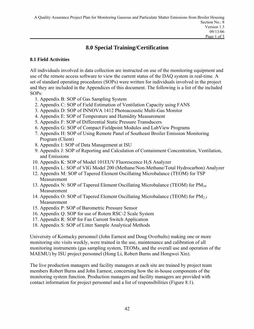
8.0 Special Training/Certification 8.1 Field Activities All individuals involved in data collection are instructed on use of the monitoring equipment and use of the remote access software to view the current status of the DAQ system in real-time. A set of standard operating procedures (SOPs) were written for individuals involved in the project and they are included in the Appendices of this document. The following is a list of the included SOPs:
1. Appendix B: SOP of Gas Sampling System 2. Appendix C: SOP of Field Estimation of Ventilation Capacity using FANS 3. Appendix D: SOP of INNOVA 1412 Photoacoustic Multi-Gas Monitor 4. Appendix E: SOP of Temperature and Humidity Measurement 5. Appendix F: SOP of Differential Static Pressure Transducers 6. Appendix G: SOP of Compact Fieldpoint Modules and LabView Programs 7. Appendix H: SOP of Using Remote Panel of Southeast Broiler Emission Monitoring
Program (Client) 8. Appendix I: SOP of Data Management at ISU 9. Appendix J: SOP of Reporting and Calculation of Containment Concentration, Ventilation,
and Emissions 10. Appendix K: SOP of Model 101EUV Fluorescence H2S Analyzer 11. Appendix L: SOP of VIG Model 200 (Methane/Non-Methane/Total Hydrocarbon) Analyzer 12. Appendix M: SOP of Tapered Element Oscillating Microbalance (TEOM) for TSP
Measurement 13. Appendix N: SOP of Tapered Element Oscillating Microbalance (TEOM) for PM10
Measurement 14. Appendix O: SOP of Tapered Element Oscillating Microbalance (TEOM) for PM2.5
Measurement 15. Appendix P: SOP of Barometric Pressure Sensor 16. Appendix Q: SOP for use of Rotem RSC-2 Scale System 17. Appendix R: SOP for Fan Current Switch Application 18. Appendix S: SOP of Litter Sample Analytical Methods
University of Kentucky personnel (John Earnest and Doug Overhults) making one or more monitoring site visits weekly, were trained in the use, maintenance and calibration of all monitoring instruments (gas sampling system, TEOMs, and the overall use and operation of the MAEMU) by ISU project personnel (Hong Li, Robert Burns and Hongwei Xin). The live production managers and facility managers at each site are trained by project team members Robert Burns and John Earnest, concerning how the in-house components of the monitoring system function. Production managers and facility managers are provided with contact information for project personnel and a list of responsibilities (Figure 8.1).
42

A Quality Assurance Project Plan for Monitoring Gaseous and Particulate Matter Emissions from Broiler Housing Section No.: 8
Version 1.3 09/13/06
Page 2 of 3 Dates of the trainings, a list of participants, and the topics included are recorded and filed by the QA Manager each time a session occurs. Because there is a high turnover rate for production facility managers, training sessions are held and recorded on an as-needed basis. 8.2 Laboratory Activities Laboratory activities for this project include archiving, reviewing, and processing of data and litter sample analysis. SOPs for managing and processing emissions data are included in the following Appendices:
1. Appendix I: SOP of Data Management at ISU 2. Appendix J: SOP of Reporting and Calculation of Containment Concentration, Ventilation,
and Emissions 3. Appendix S: SOP of Litter Sample Analytical Methods
Hong Li is handling all the data management and processing activities. For a description of his qualifications and training that has prepared him to work in this area, please see Section 4.3 of this document. Nurun Nahar is the laboratory manager for the Agricultural Waste Management Laboratory in the Department of Agricultural and Biosystems Engineering at Iowa State University. She is responsible for training individuals who work in the laboratory as well as providing sample handling and analysis oversight. Nurun Nahar trains the research assistants to run each method they work with. Additionally, all individuals working in the Agricultural Waste Management Laboratory in the Department of Agricultural and Biosystems Engineering at Iowa State University are required to complete the following trainings through Environmental Health and Safety at Iowa State University:
1. Fire Safety Emergency On-Line Training 2. Hazardous Waste Generator Training 3. Knowing How to Practice Safe Science 4. OHSA Laboratory Standard
Records of training completion are maintained by the laboratory manager. Training for use of specific methods and sample handling practices within the Agricultural Waste Management Laboratory are provided and documented by the laboratory manager. Documentation includes dates of the trainings, a list of participants, and the topics included each time a session occurs.
43
A Quality Assurance Project Plan for Monitoring Gaseous and Particulate Matter Emissions from Broiler Housing Section No.: 8
Version 1.3 09/13/06
Page 3 of 3
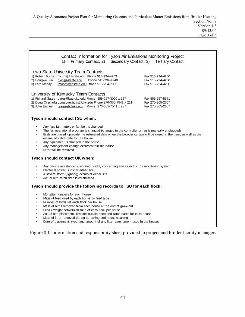
Contact Information for Tyson Air Emissions Monitoring Project 1) = Primary Contact, 2) = Secondary Contact, 3) = Tertiary Contact
Iowa State University Team Contacts 1) Robert Burns [email protected] Phone 515-294-4203 Fax 515-294-4250 2) Hongwei Xin [email protected] Phone 515-294-4240 Fax 515-294-4250 3) Lara Moody [email protected] Phone 515-294-7355 Fax 515-294-4250
University of Kentucky Team Contacts 1) Richard Gates [email protected] Phone 859-257-3000 x 127 Fax 859-257-5671 2) Doug Overhults [email protected] Phone 270-365-7541 x 211 Fax 270-365-2667 3) John Earnest [email protected] Phone 270-365-7541 x 237 Fax 270-365-2667
Tyson should contact ISU when:
• Any fan, fan motor, or fan belt is changed • The fan operational program is changed (changed in the controller or fan is manually unplugged) • Birds are placed - provide the estimated date when the brooder curtain will be raised in the barn, as well as the
estimated catch date for the house • Any equipment is changed in the house • Any management change occurs within the house • Litter will be removed
Tyson should contact UK when:
• Any on-site assistance is required quickly concerning any aspect of the monitoring system • Electrical power is lost at either site • A severe storm (lighting) occurs at either site • Actual bird catch date is established
Tyson should provide the following records to ISU for each flock:
• Mortality numbers for each house • Mass of feed used by each house by feed type • Number of birds set each flock per house • Mass of birds removed from each house at the end of grow-out • Feed / weight conversion ratio of each flock per house • Actual bird placement, brooder curtain open and catch dates for each house • Mass of litter removed during de-caking and house cleaning • Date of placement, type, and amount of any litter amendment used in the houses
Figure 8.1. Information and responsibility sheet provided to project and broiler facility managers.
44

A Quality Assurance Project Plan for Monitoring Gaseous and Particulate Matter Emissions from Broiler Housing Section No.: 9
Version 1.3 09/13/06
Page 1 of 4
9.0 Documents and Records 9.1 QAPP Distribution Following EPA’s approval of the QAPP, the plan will be distributed in both an electronic and paper document to all individuals on the QAPP distribution list included in Section 3.0: QAPP Distribution List. In addition, a bound paper copy of the current approved QAPP will be maintained in each MAEMU as an on-site reference. The QAPP has a date and version number to keep track of the most updated version.
9.2 QAPP Updates
As the project progresses it is anticipated there will be instances where changes to some SOPs and/or data acquisition and collection methods would result in improved data quality. Where the need for such changes is demonstrated, the QAPP will be updated to reflect the improved operational methods. The QAPP format is prepared so individual sections can be updated and replaced without revising the entire document. When a section is revised, a new date and version number will be assigned to that section. All updated sections of the QAPP will be distributed electronically via email to all persons included on the QAPP distribution list included in Section 3.0: QAPP Distribution List. In addition, the reference copy of the QAPP maintained in each MAEMU will be updated with the revised section. Before distribution of the updated sections, the revisions will be reviewed by the Project Investigators. Following their review, the revised sections will be submitted to the EPA Project Manager and QA Officer for approval. Because of the QAPP format, individual sections can be reviewed and approved without revising the whole document.
9.3 Identification and Recording of Project Records
In addition to the QAPP, records associated with this project include data generated on-site for gaseous and particulate matter emission rate determination, instrument calibration and maintenance records, quality control sample records, litter sample chain of custody and result records, weekly site visit reports, flock records (for example, number of birds per flock, in and out dates, and mortalities), quality control reports, and corrective action reports. For further information about the records to be maintained see Table 9.1 and Section 20: Data Management. Records resulting from this project will be retained for a period of not less than seven years following the end of the project. It is the responsibility of the lead PI, Robert Burns, to oversee archiving and disposal of all project records. Data archival and retrieval for all electronic data are covered in Section 20.9.
Emission Related Data All emissions data and records collected for this project are maintained at ISU. All electronic records are maintained in redundancies to ensure that no data will be lost because of computer theft or failures or unforeseeable natural disasters (fire, flood, etc.). Monitoring data redundancies begin at the field monitoring site in the MAEMU.
45

A Quality Assurance Project Plan for Monitoring Gaseous and Particulate Matter Emissions from Broiler Housing Section No.: 9
Version 1.3 09/13/06
Page 2 of 4
Table 9.1. Project record identification and handling. Record Type Retention Archival Disposal On-site gaseous and particulate matter emission data
Electronic database
On-site computer and ISU computer
ISU computer Records will be kept for at least 7 years after end of the project
Instrument calibration and maintenance
Paper database Original database kept on-site, copies maintained at ISU
ISU paper files Records will be kept for at least 7 years after end of the project
Quality control records
Electronic and paper database
ISU computer and ISU paper files
ISU computer and ISU paper files
Records will be kept for at least 7 years after end of the project
Litter sample results
Electronic database
ISU computer ISU computer Records will be kept for at least 7 years after end of the project
Litter sample chain of custody
Paper database ISU paper files ISU paper files Records will be kept for at least 7 years after end of the project
Site visit reports Electronic database
UK computer and ISU computer
ISU computer Records will be kept for at least 7 years after end of the project
Flock information Electronic and paper database
ISU computer and ISU paper files
ISU computer and ISU paper files
Records will be kept for at least 7 years after end of the project
Quality control reports
Electronic database
ISU computer ISU computer Records will be kept for at least 7 years after end of the project
Corrective actions Electronic and paper database
ISU computer and ISU paper files
ISU computer and ISU paper files
Records will be kept for at least 7 years after end of the project
Raw data are collected and stored on memory in the National Instruments Compact Field Point Modules. Raw data are automatically transferred to a dedicated PC located in each MAEMU. This PC performs pre-processing of data to calculate values required for emissions determinations. The raw data are automatically emailed each day at midnight to a computer dedicated to project data storage located at ISU. The pre-processed data are automatically downloaded from the MAEMU PC to the dedicated ISU project computer each day at 2:00 p.m. Following data quality review, final processing to calculate emissions is completed at ISU by the project personnel. Additionally, the University of Kentucky (UK) personnel archive both raw and pre-processed data from the MAEMU PC to a data storage CD on a weekly basis during their site checks/inspections. A designated PC at ISU processes the electronic data downloaded from on-site computers. Information on the data handling is detailed in Section 20: Data
46

A Quality Assurance Project Plan for Monitoring Gaseous and Particulate Matter Emissions from Broiler Housing Section No.: 9
Version 1.3 09/13/06
Page 3 of 4 Management. In order to reduce the level of manual data processing, automated systems are utilized where appropriate. In order to provide a backup, a hardcopy of the automated data collection information is stored for the appropriate time frame in project files. Following data quality review, final processing to calculate emissions is completed at ISU by the project personnel. The University of Kentucky personnel prepare written notes in Microsoft Word following each site visit to document all activities and observations made during the visit. These weekly site visit notes include the results of each week’s Quality Control instrument calibration and checks with calibration gas. These notes are distributed by email to the entire project team on a weekly basis. In addition, these notes are archived in an electronic format at ISU. A calibration record notebook is also maintained at each MAEMU. Records of each required instrument calibration are entered into this notebook during calibration events for each instrument. Following each flock, UK personnel photocopy these calibration records and submit them to ISU personnel, who maintain a paper copy and archive them electronically by entering the records into an electronic format. Originals of all calibration data are maintained in the on-site notebook. As necessary, manual entry field logs are maintained including, but not limited to, site drawings, daily notes about the monitoring operation and the production buildings, results of field quality control measures, and any deviations from this QAPP. These records are to be recorded with a pen only. Copies of this data will be provided to ISU at the end of each flock. Litter Sampling Data A hard copy of litter sample collection records will be maintained in a file at ISU by the Department of Agricultural and Biosystems Engineering Department’s Agricultural Waste Management Laboratory manager. Each sample is shipped with a Chain of Custody form that includes the sampler name, sample ID (which provides sample location information), and sample date and volume (see Section 13 for the Chain of Custody form and Section 12 for sample collection method, diagram and collection location information). Quality Control for laboratory analysis is described in Section 14, records of Quality Control are maintained in the laboratory by the lab manager. The SOPs for the Analytical Methods are included in Appendix S. For each set of analyses provided to the project team, the laboratory manager will provide a report including a sample handling summary and quality control data. Analysis data will be provided and maintained electronically for a period of 7 years. Production Data As part of the project, some production information is being collected. Tyson Foods maintains production records concerning consumed feed weights, broiler market weights, mortalities within each grow-out, and feed conversion rates. ISU monitors water use in the house and will analyze the litter for nutrient content. UK personnel will collect daily bird weight data and feed weight data and submit it to ISU at the end of each flock. This data will be submitted to ISU and maintained electronically. The Tyson production manager at each facility is to record certain activities at the facility that affect air quality in the production house, (for example, generator
47

A Quality Assurance Project Plan for Monitoring Gaseous and Particulate Matter Emissions from Broiler Housing Section No.: 9
Version 1.3 09/13/06
Page 4 of 4 tests, manure removals, change in diet and animal health, house temperature set points, ventilation interventions, building cleaning, and power failures). See Appendix A for SOP. 9.4 Data Correction When records are reviewed, corrections may be required. If any member of the project team needs to perform a data correction, the proposed correction must first be reviewed by a project PI, not including the individual performing the data correction. Corrections to electronic data will be noted and provided in the mid-term and final emissions report. Corrections to hand written documents will be added and initialed by the individual making the correction. All data corrections will be recorded in a corrective action report.
48

A Quality Assurance Project Plan for Monitoring Gaseous and Particulate Matter Emissions from Broiler Housing Section No.: 10
Version 1.3 09/13/06
Page 1 of 1
10.0 Biosecurity Plan Biosecurity refers to a set of management practices that reduce the potential for the introduction or spread of disease-causing organisms onto and between sites. Disease carriers can be anything and/or anybody that comes in contact with infected animals, materials or equipment. Bacterial or viral particles transmitted by animals can survive for variable lengths of time almost anywhere under normal environmental conditions. A person or item can become a disease carrier when it comes into contact with contaminated materials such as feces, bedding or air within the area. When a non-disinfected contaminated source leaves one environment and enters another (for example, enters a vehicle to leave the facility), the new area becomes contaminated (Hill, 2003). Standard operating procedures for the broiler houses in this study require biosecurity practices to be in place that are designed to eliminate, contain, or reduce the exposure and spread of poultry pathogens. For this project, three levels of biosecurity management practices will be in place. Stage 1 procedures should be in place under normal conditions when no disease is present locally or in adjacent regions. Stage 2 procedures should be in place when a disease is present locally or in an adjacent region. Stage 3 procedures should be in place when a disease is present on the farm or a severe disease is present in the immediate area. During Stage 1 conditions (normal operation), individuals on the project team wear clean clothes and footwear when entering the farm. Personnel wear protective boots, coveralls, hair hats, and gloves. Clothing will not be used at different sites. Shoes are covered with either washable rubber boots or disposable plastic boots. If disposable boots are worn, the used materials are left on the farm. If washable boots are worn, the boots are disinfected before departing the facility. Individuals wash hands before leaving the farm; acceptable methods include waterless gels, disinfecting hand wipes, or soap and water. All reusable equipment leaving the facility is cleaned and disinfected. Vehicle tires and wheel wells are sprayed with a bio-disinfectant both when arriving and departing the site. Vehicles remain parked in one location until departure from the sight. During Stage 2 conditions (no disease on site, but disease present in surrounding areas), individuals follow all of the procedures described above, as well as develop a log of visits to and from the two facilities in chronological order. During Stage 3 conditions (a disease on-site) project team members restrict all visits to the facility, unless a site visit is mandatory. In the case of a site visit during this stage of operation, the visit must be approved by the live production manager. If an individual must visit the facility during this time, they arrive with a prepared biosecurity kit. The kit contains disposable coveralls, boots, hair nets, gloves, hand sanitation items, paper towels, and trash bags in a sealed plastic container. All disposable items must be double-bagged and left on the farm site. Any samples leaving the farm must be double-bagged. The individual’s vehicle should be emptied of all nonessential items before arriving at the farm.
49

A Quality Assurance Project Plan for Monitoring Gaseous and Particulate Matter Emissions from Broiler Housing Section No.: 11
Version 1.3 09/13/06
Page 1 of 13
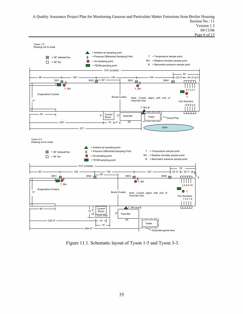
11.0 Sampling Process Design 11.1 Measurement of Gaseous and Particulate Matter Concentrations The basis for the sampling design of this monitoring is continuous measurement of gaseous and particulate pollutant concentrations and the corresponding building ventilation rates to determine the pollutant emission rate (ER) from two commercial broiler houses for one year. The gases and particulate matter (PM) measured in this project include NH3, H2S, CO2, non-methane hydrocarbons (NMHC), total suspended particulates (TSP), PM10 and PM2.5. Two broiler houses, each measuring 13.1 m × 155.5 m (43 × 510 ft) and built in the early 1990s, are being monitored at two farm sites 40 miles apart in western Kentucky. Characteristics for each site are included in Table 11.1. Each house has an initial placement of 25,800 Cobb-Cobb straight-run (mixed sex) broilers in winter and 24,400 in summer, generally grown to 53 days of market age. The houses feature insulated drop ceilings (about R19), box air inlets (15 × 66 cm each) along the sidewalls (26 per sidewall), 26 pancake brooders (8.8 kW or 30,000 Btu/hr each), three space furnaces (65.9 kW or 225,000 Btu/hr each), four 91-cm (36-in) diameter sidewall exhaust fans spaced about 120 ft apart, and ten 123-cm (48-in) diameter tunnel fans. The 91-cm (36-in) fan (SW1) for minimum ventilation is located in the brood end of the houses. Two 24-m (80-ft) sections of evaporative cooling pads are located in the opposite end of the tunnel fans. The houses are also equipped with foggers for additional cooling, if needed. A mixture of rice hulls and sawdust is used as litter bedding. Air samples are drawn from three locations in each house as well as from an outside location to provide ambient background data (Figure 11.1). One sampling location is near the primary minimum ventilation (36-in) sidewall fan (SW1) used for cold weather ventilation (in the brooding half of the house). The second sampling location is near the fourth sidewall (36-in) exhaust fan (SW3) (non-brooding end). The third location is at the tunnel end (TE). The ambient sample location (A) is between the inlet boxes opposite of the sidewall with the exhaust fans. The quantity of gas in the background (for example, inlet air) is subtracted from that in the exhaust air when calculating aerial emissions from the house. Placement of the air sampling ports are as follows: for the two sidewall sampling locations, the sampling ports and temperature sensors are located 1.2 m (4.0 ft) away from the fan in the axial direction, 2.3 m (7.5 ft) in the radial direction, and 1 m (3 ft) above the floor; for the tunnel-end sampling location, the sampling port and temperature sensor is located at the center across the house (for example, 6.6 m or 21.5 ft from each sidewall) and 7.3 m (24.0 ft) from the end wall. Figure 11.2 shows the axial and vertical location of the sampling points in relation to the fan centers. Sampling locations and placement of the sampling ports were chosen to maximize representation of the air leaving the houses. Each sample inlet point is equipped with a dust filter to keep large particulate matter from plugging the sample tubing. The schedules of sampling events and sequences are as follows (refer to Figure 11.3). If the ventilation fans at the three in-house sampling locations (SW1-location 1, SW3-location 2 and
50

A Quality Assurance Project Plan for Monitoring Gaseous and Particulate Matter Emissions from Broiler Housing Section No.: 11
Version 1.3 09/13/06
Page 2 of 13 TE-location 3) are all running, air samples from each location are analyzed sequentially via the controlled operation of the servo values in the gas sampling system (GSS). In this case, sampling/analysis sequence is SW1, SW2, and TE, and the cycle repeats. The time of analysis per sampling episode for each location is 120 seconds, involving four consecutive 30-second readings by the INNOVA 1412 multi-gas analyzer (INNOVA model 1412, INNOVA AirTech Instruments A/S, Denmark). The fourth reading is considered to be the equilibrium value of the location and used in the subsequent analysis of emission rate. The selection of the 120-second sample analysis time is based on extensive laboratory tests and field verification with calibration gases and concurrent measurement of the sampling location by INNOVA 1412 analyzers located inside the house and inside the MAEMU. A UV Fluorescence H2S analyzer (Model 101E, Teledyne API, San Diego, CA) is a microprocessor controlled analyzer that determines the concentration of hydrogen sulfide (H2S). The 95% response time of the API 101E is shorter than 100 seconds. According to the response time of INNOVA 1412, the last H2S readings correlated to the four INNOVA cycles were used for H2S emission calculation. The VIG model 200 methane/non-methane/total hydrocarbon analyzer (Model 200, VIG Industries Inc., Anaheim, CA) uses column technology to separate methane and non-methane from total hydrocarbons and uses a dual FID (flame ionization detector) to measure each component in the air sample. The response time of non-methane hydrocarbon (NMHC) is 70 seconds and NMHC reading was updated every 3 minutes. Every NMHC reading from the VIG 200 analyzer was identified with the corresponding sampling location and used for the emission calculation. If fans at SW3 or TE are not running (for example, during half-house brood), sample analysis will repeat for the SW1 location only, and the same is true for TE sampling when fans at SW1 and SW3 are not running (for example, during tunnel ventilation mode). Every two hours, air samples from the ambient (background) location are drawn and analyzed for 8 minutes. The longer sample analysis time for the ambient point is a result of the longer response time of the instrument when measuring a large step change in gas concentration. Selection of a 2-hour interval for the analysis of the ambient concentrations is because of the fact that ambient conditions remain relatively constant, as compared to the in-house conditions. Such an arrangement helps maximize the number of data points collected for the exhaust air and thus, house emissions.
The sequential sampling makes the assumption that any concentration changes at the given location during the two adjacent measurements (generally 360 seconds) follow a linear pattern. Hence, linear interpolation from the two measured values is used to determine intermediate values for the location, as needed. Use of one sampling location at the tunnel fan end also assumes homogeneity in distribution of aerial concentrations. Examination of ammonia concentrations across the house in this section, through concurrent measurements using four INNOVA 1412 analyzers, has confirmed the validity of this assumption. Moreover, it was assumed that the vertical stratifications in aerial concentrations are negligible when the exhaust fans are in operation. Once again, this assumption has been verified by concurrent measurements of vertical distribution of ammonia and CO2 concentrations (from floor to ceiling). Incidentally, appreciable vertical stratifications exist when the fans are off. For measurement of emissions, we are only concerned with the concentrations that correspond to operation of the fans.
51

A Quality Assurance Project Plan for Monitoring Gaseous and Particulate Matter Emissions from Broiler Housing Section No.: 11
Version 1.3 09/13/06
Page 3 of 13 Air samples will be collected via 0.95-cm (3/8-inch) o.d. and 0.64-cm (1/4-inch) i.d. Teflon tubing (Fluorotherm FEP tubing). Individual supply pumps (with all internal wetted parts Teflon coated) are used to continuously draw air from each of the sampling locations. Use of individual pumps dedicated to each sampling location eliminates potential residual effects from sharing pumps among sampling locations, this is especially the case between ambient/background air and in-house exhaust air samples. The sampling scheme is designed such that air is continuously drawn from all four sampling points. When a sample point is not being analyzed, the flow is bypassed from the instrument in the MAEMU. This arrangement is designed to minimize the residence time and thus, the sample-to-sample purging time. Considerable discussion and investigation has gone into the placement of the Tapered Element Oscillating Microbalance (TEOM) particulate matter samplers (TSP, PM10, PM2.5) in the house. Since no data was available in terms of TEOM responses to different air velocity fields, as would be encountered in the broiler houses, we conducted an in-house evaluation of the TEOM performance for air velocity ranging from 1.3 – 6 m⋅s-1 (250 to 1200 feet per minute). The results revealed that the TEOM readings are unaffected by the tested air velocity range. Prior to the TEOM tests, we had assumed continuity in PM concentrations from the center of the house to the exhaust. Since we were concerned that the TEOMs might not function properly under high velocity conditions near the exhaust fan, we placed the TEOMs near the center, across the width of the house. Comparison of two TEOM readings near the center versus near the exhaust of the house, revealed that concentrations near the exhaust were generally lower than concentrations near the center. Since velocity showed no impact on the concentration measurement and we are to quantify the emissions going out of the house, we located the TEOMs near the exhaust fan(s). The specifics of TEOM placement are as follows. During the half-house brooding period, the TEOMs are placed near SW1. The TSP TEOM is located 0.6 m (2.0 ft) away from the fan in the axial direction, 1.1 m (3.5 ft) in the radial direction to the left of the fan, and 1.5 m (5.0 ft) above the floor. The PM10 TEOM is located 0.6 m (2.0 ft) away from the fan in the axial direction, 1.1 m (3.5 ft) in the radial direction to the right of the fan, and 1.5 m (5.0 ft) above the floor. The PM2.5 TEOM is located 0.6 m (2.0 ft) away from the fan in the axial direction, 2.2 m (7.0 ft) in the radial direction to the right of the fan, and 1.5 m (5.0 ft) above the floor. Once the birds are given the full house (between 10-14 days of age), the TEOMs are moved to the TE location. For the TE sampling location, the TSP TEOM is located 4.9 m (16.0 ft) away from the tunnel fan in the axial direction, 11 m (36 ft) from the tunnel end of the house, and 1.5 m (5.0 ft) above the floor. The PM10 TEOM is located 4.9 m (16.0 ft) away from the tunnel fan in the axial direction, 9.8 m (32.0 ft) from the tunnel end of the house, and 1.5 m (5.0 ft) above the floor. The PM2.5 TEOM is located 4.9 m (16.0 ft) away from the tunnel fan in the axial direction, 8.5 m (28.0 ft) from the tunnel end of the house, and 1.5 m (5.0 ft) above the floor. All the sampling locations are accessible, although some are relatively easier than others when placing the TEOM units. Tables 11.2 and 11.3 summarize the variables monitored, the instruments used, and the sampling intervals, for easy reference.
52

A Quality Assurance Project Plan for Monitoring Gaseous and Particulate Matter Emissions from Broiler Housing Section No.: 11
Version 1.3 09/13/06
Page 4 of 13
Table 11.1. Characteristics of the broiler houses monitored. Site 1-5 Site 3-3 Species Broilers Broilers # Buildings at site 8 24 Year of buildings 1992 1991 Ridgeline orientation North-South North-South Building type litter litter Manure storage, days ~ 1 year ~ 1 year Animal residence time, days 53 53 Outdoor storage none none Mortality disposal Composting Composting Spacing, ft 60 60 Ridge height, ft 17.2 17.2 Sidewall height, ft 7 7 # air inlets 52 52 Type of inlet Box Box Inlet control method automatic automatic # fans/bldg or room 14 14 Largest fan diameter, in. 48 48 Smallest fan diameter, in. 36 36 # ventilation stages 12 13 Fan company CanArm Euroemme Controls company Chore-Time Rotem Artificial heating? Yes Yes Summer cooling EP/tunnel EP/tunnel Brooding section South half of barn South half of barn 24/7 internet Satellite Satellite Distance to site, mi. 30 miles 18 miles Inventory/building 24,400 (summer)
25,800 (winter) 24,400 (summer) 25,800 (winter)
Building width, ft 43 43 Building length, ft 510 510 Building area, ft2 21,930 21,930 Shower in/out? Not required Not Required Start date January 2006 January 2006 Completion date January 2007 January 2007
53
A Quality Assurance Project Plan for Monitoring Gaseous and Particulate Matter Emissions from Broiler Housing Section No.: 11
Version 1.3 09/13/06
Page 5 of 13
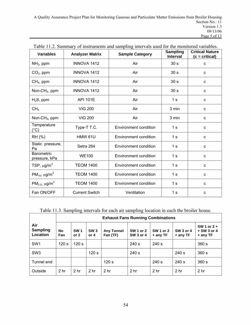
Table 11.2. Summary of instruments and sampling intervals used for the monitored variables. Variables Analyzer Matrix Sample Category Sampling
Interval Critical Nature
(c = critical) NH3, ppm INNOVA 1412 Air 30 s c
CO2, ppm INNOVA 1412 Air 30 s c
CH4, ppm INNOVA 1412 Air 30 s c
Non-CH4, ppm INNOVA 1412 Air 30 s c
H2S, ppm API 101E Air 1 s c
CH4 VIG 200 Air 3 min c
Non-CH4, ppm VIG 200 Air 3 min c Temperature (°C) Type-T T.C. Environment condition 1 s c
RH (%) HMW 61U Environment condition 1 s c Static pressure, Pa Setra 264 Environment condition 1 s c Barometric pressure, kPa WE100 Environment condition 1 s c
TSP, μg/m3 TEOM 1400 Environment condition 1 s c
PM10, μg/m3 TEOM 1400 Environment condition 1 s c
PM2.5, μg/m3 TEOM 1400 Environment condition 1 s c
Fan ON/OFF Current Switch Ventilation 1 s c
Table 11.3. Sampling intervals for each air sampling location in each the broiler house. Exhaust Fans Running Combinations
Air Sampling Location
No Fan
SW 1 or 2
SW 3 or 4
Any Tunnel Fan (TF)
SW 1 or 2SW 3 or 4
SW 1 or 2+ any TF
SW 3 or 4 + any TF
SW 1 or 2 + + SW 3 or 4 + any TF
SW1 120 s 120 s 240 s 240 s 360 s
SW3 120 s 240 s 240 s 360 s
Tunnel end 120 s 240 s 240 s 360 s
Outside 2 hr 2 hr 2 hr 2 hr 2 hr 2 hr 2 hr 2 hr
54
A Quality Assurance Project Plan for Monitoring Gaseous and Particulate Matter Emissions from Broiler Housing Section No.: 11
Version 1.3 09/13/06
Page 6 of 13
Figure 11.1. Schematic layout of Tyson 1-5 and Tyson 3-3.
22’-9” 24’-2”
Brood Curtain Evaporative Coolers
SW1 SW2 SW3 SW4
22’
12’
9 7 5 3 1 10 8 6 4 2
Fan Numbers
Feed Bin Trailer Gravel Pad
Tyson 1-5 Drawing not to scale
Ditch
T, RH T, RH
105’ 120’98’ 135’52’
5’
235’ 15’
Control Room
5’
8’
510’ (outside)
277’
52’
80’
Note: Curtain aligns with end of Feed Bin Pad.
T, RH, B
T
RH = Relative Humidity sample point
= Pressure Differential Sampling Point
= Air sampling point = 36” sidewall fan
= 48” fan
T = Temperature sample point = Ambient air sampling point
= TEOM sampling point B = Barometric pressure sample point
43’
Brood Curtain Evaporative Coolers
SW1 SW2 SW3 SW4
24’
12’
2 4 6 8 10 1 3 5 7 9
Fan Numbers
Feed Bin
Trailer
Extended gravel lane
Tyson 3-3 Drawing not to scale
ControlRoom
T, RH T, RH
T
120’ 58’
135’120’83’ 24’-7” 22’-5” 52’
5’
510’ (outside)
80’
235’-6”
Conc Pad
10’
15’
8’ 14’
284’-6”’
Note: Curtain aligns with end of Feed Bin Pad.
RH = Relative Humidity sample point
= Pressure Differential Sampling Point
= Air sampling point = 36” sidewall fan
= 48” fan
T = Temperature sample point = Ambient air sampling point
= TEOM sampling point
T, RH and B
B = Barometric pressure sample point
43’
55

A Quality Assurance Project Plan for Monitoring Gaseous and Particulate Matter Emissions from Broiler Housing Section No.: 11
Version 1.3 09/13/06
Page 7 of 13
Figure 11.2. Cross sectional view of the sidewall sampling points.
Location 3
Location 2
Location 1
Ambient air
P 4
P 3
P 2
P 1
M1
S1
S5
S2
S3
S4
S6
S7
S8
Exhaust
Compact Fieldpoint DAQ
Filter Filter
Red line: heated line
ExhaustM2
INNOVA 1412
API 101E
VIG 200
Flow meter
P: PumpM: Manifold S1- 4: Normal Closed
Location 3
Location 2
Location 1
Ambient air
P 4
P 3
P 2
P 1
M1
S1
S5
S2
S3
S4
S6
S7
S8
Exhaust
Compact Fieldpoint DAQ
Filter Filter
Red line: heated line
ExhaustM2
INNOVA 1412
API 101E
VIG 200
Flow meter
P: PumpM: Manifold S1- 4: Normal Closed
Figure 11.3. Schematic representation of the positive pressure GSS used in the MAEMU for measurement of broiler house air emissions. The GSS features continuous drawing of sample air
from all locations with individual pumps. The sample air is bypassed when not analyzed.
1.3 m (4.3 ft) 1.2 m (3.8 ft)
2.1m (7.0 ft)
0.9 m (3.0 ft Fan) 1.2 m
(4.0ft Fan)
Floor
Ceiling
= Sampling point
Cross-section View
0.9 m (3.0 ft)
1.2 m (4.0 ft)
0.9 m (3.0 ft)
Top View
2.3 m (7.5 ft)
1.2 m (4.0 ft)
56

A Quality Assurance Project Plan for Monitoring Gaseous and Particulate Matter Emissions from Broiler Housing Section No.: 11
Version 1.3 09/13/06
Page 8 of 13 11.2 Measurement of Ventilation Rate Ventilation rates of the houses are measured using the following procedure. First, all exhaust fans have been calibrated in situ, with a state-of-the-art Fan Assessment Numeration System (FANS) to obtain the actual ventilation curves (airflow rate versus static pressure). Guidelines for FANS calibration are presented in Appendix C. This calibration is essential for accurate measurement of the house ventilation rate because actual fan airflow rates can differ by 10-25% as compared with the default values provided by the fan manufacturer. The deviation arises from the field operational conditions that differ drastically from those under which the default values were established (for example a loose motor belt or dirty shutters or fan blades). Runtime of each fan is monitored continuously using an inductive current switch (with analog output) attached to the power supply cord of each fan motor (Figure 11.5) as described in Appendix R, and recorded by the compact Fieldpoint modules as described in Appendix G. Concurrent measurement of the house static pressure is made with two static pressure sensors (Model 264, Setra, Boxborough, MA), each for half of the house. While the pressure differential is not expected to differ at the two locations, two sensors are used to provide redundancy in this critical measurement. Summation of airflows from the individual fans during each monitoring cycle or sampling interval produces the overall house ventilation rate. This method of determining dynamic ventilation rates of mechanically ventilated animal confinement has been successfully used in recent AFO air emission studies in the United States.
Variation in airflow rates among 0.9-m (36 inch) and 1.2-m (48 inch) fans, as measured with the FANS
0
2000
4000
6000
8000
10000
12000
14000
16000
18000
0 0.02 0.04 0.06 0.08 0.1 0.12 0.14 0.16 0.18Static Pressure, inch WC
Fan
airf
low
rate
, cfm
48" fans
36" fans
1 cfm = 1.7 m3/hr
1 inch WC = 248.9 pa
Figure 11.4. Variation in the fan airflow rates among the 36-in and 48-in fans
in a Tyson broiler house. At the beginning of the project, all 14 ventilation fans in each house were calibrated and fan curves were developed. Afterward, three to four fans in each house (less than 20% of total fans) were randomly chosen and tested at the beginning of each flock. If airflow rates of the randomly selected fans deviate from the initial calibration values by 10% or greater, all fans will be
57
A Quality Assurance Project Plan for Monitoring Gaseous and Particulate Matter Emissions from Broiler Housing Section No.: 11
Version 1.3 09/13/06
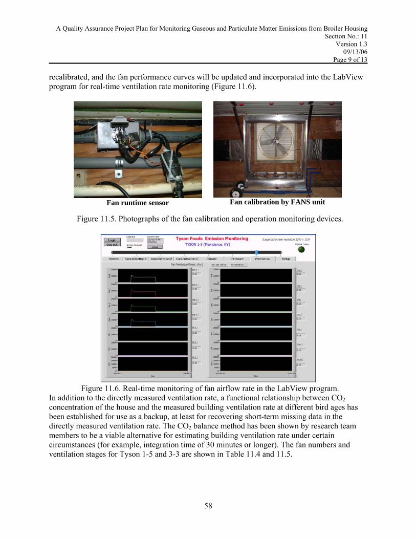
Page 9 of 13 recalibrated, and the fan performance curves will be updated and incorporated into the LabView program for real-time ventilation rate monitoring (Figure 11.6).
Fan runtime sensor
Fan calibration by FANS unit
Figure 11.5. Photographs of the fan calibration and operation monitoring devices.
Figure 11.6. Real-time monitoring of fan airflow rate in the LabView program.
In addition to the directly measured ventilation rate, a functional relationship between CO2 concentration of the house and the measured building ventilation rate at different bird ages has been established for use as a backup, at least for recovering short-term missing data in the directly measured ventilation rate. The CO2 balance method has been shown by research team members to be a viable alternative for estimating building ventilation rate under certain circumstances (for example, integration time of 30 minutes or longer). The fan numbers and ventilation stages for Tyson 1-5 and 3-3 are shown in Table 11.4 and 11.5.
58
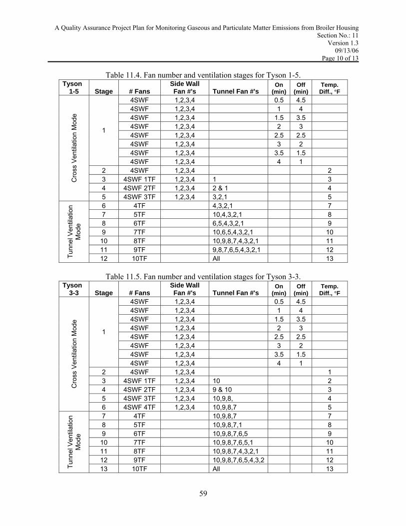
A Quality Assurance Project Plan for Monitoring Gaseous and Particulate Matter Emissions from Broiler Housing Section No.: 11
Version 1.3 09/13/06
Page 10 of 13
Table 11.4. Fan number and ventilation stages for Tyson 1-5. Tyson
1-5 Stage # Fans Side Wall Fan #'s Tunnel Fan #'s
On (min)
Off (min)
Temp. Diff., °F
4SWF 1,2,3,4 0.5 4.5 4SWF 1,2,3,4 1 4 4SWF 1,2,3,4 1.5 3.5 4SWF 1,2,3,4 2 3 4SWF 1,2,3,4 2.5 2.5 4SWF 1,2,3,4 3 2 4SWF 1,2,3,4 3.5 1.5
1
4SWF 1,2,3,4 4 1 2 4SWF 1,2,3,4 2 3 4SWF 1TF 1,2,3,4 1 3 4 4SWF 2TF 1,2,3,4 2 & 1 4
Cro
ss V
entil
atio
n M
ode
5 4SWF 3TF 1,2,3,4 3,2,1 5 6 4TF 4,3,2,1 7 7 5TF 10,4,3,2,1 8 8 6TF 6,5,4,3,2,1 9 9 7TF 10,6,5,4,3,2,1 10
10 8TF 10,9,8,7,4,3,2,1 11 11 9TF 9,8,7,6,5,4,3,2,1 12
Tunn
el V
entil
atio
n M
ode
12 10TF All 13
Table 11.5. Fan number and ventilation stages for Tyson 3-3. Tyson
3-3 Stage # Fans Side Wall Fan #'s Tunnel Fan #'s
On (min)
Off (min)
Temp. Diff., °F
4SWF 1,2,3,4 0.5 4.5 4SWF 1,2,3,4 1 4 4SWF 1,2,3,4 1.5 3.5 4SWF 1,2,3,4 2 3 4SWF 1,2,3,4 2.5 2.5 4SWF 1,2,3,4 3 2 4SWF 1,2,3,4 3.5 1.5
1
4SWF 1,2,3,4 4 1 2 4SWF 1,2,3,4 1 3 4SWF 1TF 1,2,3,4 10 2 4 4SWF 2TF 1,2,3,4 9 & 10 3 5 4SWF 3TF 1,2,3,4 10,9,8, 4
Cro
ss V
entil
atio
n M
ode
6 4SWF 4TF 1,2,3,4 10,9,8,7 5 7 4TF 10,9,8,7 7 8 5TF 10,9,8,7,1 8 9 6TF 10,9,8,7,6,5 9
10 7TF 10,9,8,7,6,5,1 10 11 8TF 10,9,8,7,4,3,2,1 11 12 9TF 10,9,8,7,6,5,4,3,2 12
Tunn
el V
entil
atio
n M
ode
13 10TF All 13
59
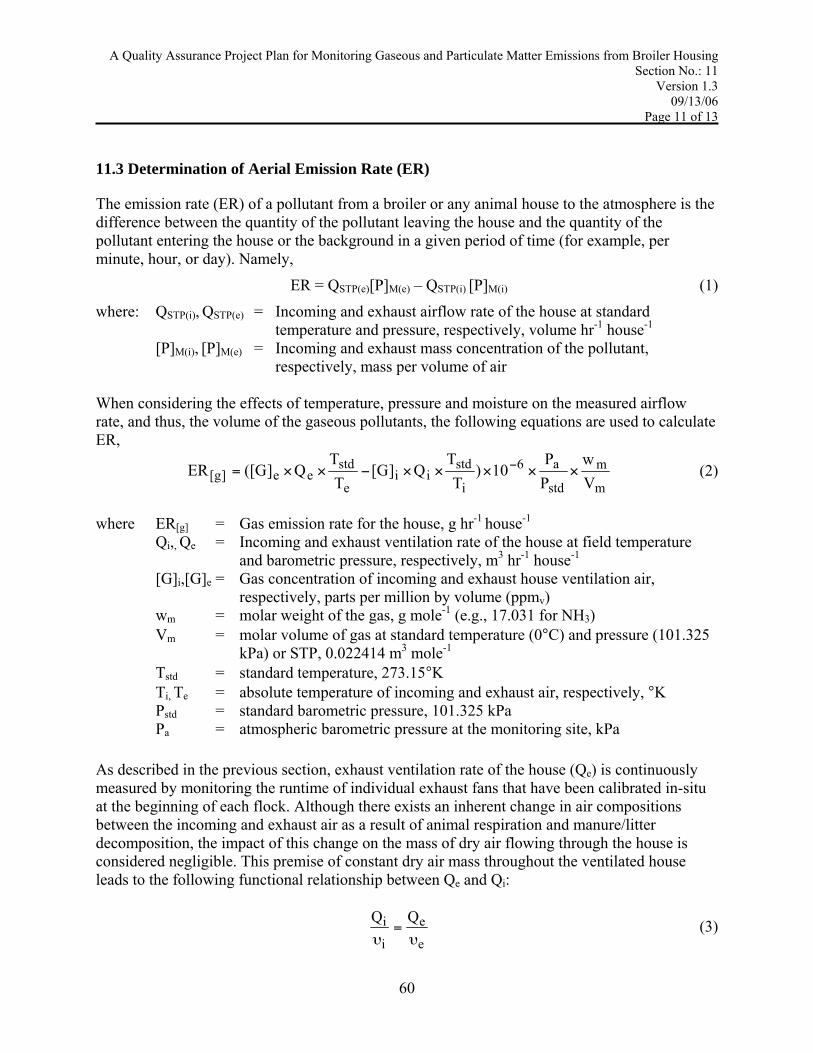
A Quality Assurance Project Plan for Monitoring Gaseous and Particulate Matter Emissions from Broiler Housing Section No.: 11
Version 1.3 09/13/06
Page 11 of 13 11.3 Determination of Aerial Emission Rate (ER) The emission rate (ER) of a pollutant from a broiler or any animal house to the atmosphere is the difference between the quantity of the pollutant leaving the house and the quantity of the pollutant entering the house or the background in a given period of time (for example, per minute, hour, or day). Namely,
ER = QSTP(e)[P]M(e) – QSTP(i) [P]M(i) (1)
where: QSTP(i), QSTP(e) = Incoming and exhaust airflow rate of the house at standard temperature and pressure, respectively, volume hr-1 house-1
[P]M(i), [P]M(e) = Incoming and exhaust mass concentration of the pollutant, respectively, mass per volume of air
When considering the effects of temperature, pressure and moisture on the measured airflow rate, and thus, the volume of the gaseous pollutants, the following equations are used to calculate ER,
m
m
std
a6
i
stdii
e
stdee]g[ V
wPP
10)T
TQ]G[
TT
Q]G([ER ×××××−××= − (2)
where ER[g] = Gas emission rate for the house, g hr-1 house-1 Qi,, Qe = Incoming and exhaust ventilation rate of the house at field temperature
and barometric pressure, respectively, m3 hr-1 house-1 [G]i,[G]e = Gas concentration of incoming and exhaust house ventilation air,
respectively, parts per million by volume (ppmv) wm = molar weight of the gas, g mole-1 (e.g., 17.031 for NH3) Vm = molar volume of gas at standard temperature (0°C) and pressure (101.325
kPa) or STP, 0.022414 m3 mole-1 Tstd = standard temperature, 273.15°K Ti, Te = absolute temperature of incoming and exhaust air, respectively, °K
Pstd = standard barometric pressure, 101.325 kPa Pa = atmospheric barometric pressure at the monitoring site, kPa As described in the previous section, exhaust ventilation rate of the house (Qe) is continuously measured by monitoring the runtime of individual exhaust fans that have been calibrated in-situ at the beginning of each flock. Although there exists an inherent change in air compositions between the incoming and exhaust air as a result of animal respiration and manure/litter decomposition, the impact of this change on the mass of dry air flowing through the house is considered negligible. This premise of constant dry air mass throughout the ventilated house leads to the following functional relationship between Qe and Qi:
e
e
i
i QQυ
=υ
(3)
60

A Quality Assurance Project Plan for Monitoring Gaseous and Particulate Matter Emissions from Broiler Housing Section No.: 11
Version 1.3 09/13/06
Page 12 of 13
where υi and υe are specific volumes of incoming and exhaust air, respectively, m3 moist air per kg dry air. Refer to Appendix J (SOP of Reporting and Calculation of Contaminant Concentrations, Ventilation and Emissions) for calculation of thermodynamic properties of the moist air. Submitting Qe into equation (2) yields the following equation for calculation of gaseous ER:
m
m
std
astd
6
i
i
e
i
e
ee]g[ V
wPP
T10)T
]G[T
]G[(QER ×××××
υ
υ−= − (4)
All the variables of pollutant concentration, fan runtime, static pressure, air temperature and relative humidity (RH) will be continuously measured and recorded at 30-second intervals throughout the one-year monitoring period. The 30-second interval of raw data will be processed to yield hourly emission rates by the following equation:
[ ]( )
( )
( )
( )
( )
( ) m
m
std
astd
6
l,ki
l,ki
l,ke
l,ki
l,ke
l,ken
1k
3
1ll,kg V
wPP
T10)T
]G[T
]G[(QER ×××××
υ
υ−= −
= =∑ ∑ (5)
where: k = number of valid concentration measurements per location within the hour l = number of sampling locations per house Qk,l = amount of airflow during the kth time period corresponding to the measured
gas concentration at lth location, m3 wm = molar weight of the gas, g mole-1 (e.g., 17.031 for NH3) Vm = molar volume of gas at standard temperature (0°C) and pressure (101.325
kPa) or STP, 0.022414 m3 mole-1 Tstd = standard temperature, 273.15°K Ti, Te = absolute temperature of incoming and exhaust air, respectively, °K Pstd = standard barometric pressure, 101.325 kPa Pa = atmospheric barometric pressure at the monitoring site, kPa υi, υe = specific volume of incoming and exhaust air, respectively, m3 moist air per kg
dry air Concentrations of the PM have the unit of μg⋅m-3. Consequently, ER of PM is calculated with the following equation:
std
astd
16.0
i
i
e
i
e
ee]PM[ P
PT10)
T]PM[
T]PM[
(QER ××××υ
υ−= − (6)
where: ER[PM] = PM (TSP, PM10, or PM2.5) emission rate for the house, kg hr-1
house-1 [PM]i, [PM]e = PM concentration of incoming and exhaust house ventilation air,
respectively, μg per m3 of air at standard temperature and pressure
61

A Quality Assurance Project Plan for Monitoring Gaseous and Particulate Matter Emissions from Broiler Housing Section No.: 11
Version 1.3 09/13/06
Page 13 of 13 11.4 Measurement of Air Temperature and Relative Humidity Indoor and outdoor temperature and RH are measured with robust and stable temperature (type T thermocouples) and RH probes (Vaisala HMW 61 units) that are connected to the PC-based data acquisition (DAQ) system (National Instruments Compact Field Point running LabView 7.1). Analog output of the static pressure sensor is connected to the DAQ system. 11.5 Litter Sampling Litter from the production houses is analyzed for nitrogen content. Litter is sampled after removal of each flock as described in Section 12.9: Litter Sampling Methods. Analyzed samples, in conjunction with litter mass removed during cleanout are used to estimate non-gaseous nitrogen movement in and out of the house. 11.6 Schedule of Peer Review Activities The sampling process design presented here incorporates extensive experience in air emission monitoring accumulated by the research team members over the years. Nonetheless, we have selected two nationally renowned experts (Dr. Jacobson and Dr. Parker) in air quality monitoring to serve as the external peer reviewers of the sampling system and protocols. Upon approval by the EPA, the on-site review by the peer experts will be conducted. The experts have been contacted and alerted about the time sensitive nature of the review, and they are prepared to perform the review in a timely manner once contacted. Prior to the site visit, the reviewers will be provided a copy of our QAPP and any additional information pertaining to the monitoring system that they may wish to have. Upon acceptance of the project QAPP by the EPA, Drs. Parker and Jacobson will be provided with the final version of the QAPP and the External Technical System Audit will be scheduled. The project team’s goal is to conduct this audit as soon as possible following the EPA approval of the QAPP. 11.7 Procedures for Coping with Sample Design Changes Any changes to the sampling system will be documented by the project team and full explanations of these changes will be included in reports to management. If any sample system design changes occur, the date and nature of the change will be documented in the notes section of the data spreadsheets so data users are aware that the change in question occurred. System design changes will also be documented in the following reports to management: On-site System Inspection Reports, Internal Technical System Audit Reports and Mid-Term Project Report. Any deviation in system maintenance or operation to ensure the integrity of the sampling system operation, and thus the data collected, will be reported to the entire research team and documented in the project logbooks in a timely and meticulous fashion. The QA Manager will be promptly notified about the changes as well.
62