7.04 Analytical Approaches to Mantle Dynamics · 7.04.4.3 Intermediate Asymptotics with Respect to Parameters: The R–T Instability 178 7.04.5 Slow Viscous Flow 179 7.04.5.1 Basic

7.04 Analytical Approaches to Mantle DynamicsN. M. Ribe, Institut de Physique du Globe, Paris, France

ª 2007 Elsevier B.V. All rights reserved.

7.04.1 Introduction 168

7.04.2 Formulating Geodynamical Model Problems: Three Case Studies 169

7.04.2.1 Heat Transfer from Mantle Diapirs 170

7.04.2.2 Plume Formation in TBLs 171

7.04.2.3 Plume–Lithosphere Interaction 172

7.04.3 Dimensional and Scaling Analysis 173

7.04.3.1 Buckingham’s �-Theorem and Dynamical Similarity 173

7.04.3.2 Nondimensionalization 174

7.04.3.3 Scaling Analysis 175

7.04.4 Self-Similarity and Intermediate Asymptotics 176

7.04.4.1 Conductive Heat Transfer 176

7.04.4.2 Classification of Self-Similar Solutions 177

7.04.4.3 Intermediate Asymptotics with Respect to Parameters: The R–T Instability 178

7.04.5 Slow Viscous Flow 179

7.04.5.1 Basic Equations and Theorems 179

7.04.5.2 Potential Representations for Incompressible Flow 181

7.04.5.2.1 2-D and axisymmetric flows 181

7.04.5.2.2 3-D flows 181

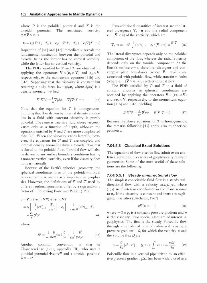
7.04.5.3 Classical Exact Solutions 182

7.04.5.3.1 Steady unidirectional flow 182

7.04.5.3.2 Stokes–Hadamard solution for a sphere 183

7.04.5.3.3 Models for subduction zones and ridges 183

7.04.5.3.4 Viscous eddies 184

7.04.5.4 Superposition and Eigenfunction Expansion Methods 185

7.04.5.4.1 2-D flow in Cartesian coordinates 185

7.04.5.4.2 Spherical coordinates 187

7.04.5.4.3 Bispherical coordinates 187

7.04.5.5 The Complex-Variable Method for 2-D Flows 188

7.04.5.6 Singular Solutions and the Boundary-Integral Representation 188

7.04.5.6.1 Flow due to point forces 188

7.04.5.6.2 Flows due to point sources 189

7.04.5.6.3 Singular solutions in the presence of a boundary 189

7.04.5.6.4 Boundary-integral representation 190

7.04.5.7 Slender-Body Theory 191

7.04.5.8 Flow Driven by Internal Loads 191

7.04.5.8.1 Wave-domain Green functions 192

7.04.5.8.2 The propagator-matrix method 194

7.04.6 Elasticity and Viscoelasticity 196

7.04.6.1 Correspondence Principles 196

7.04.6.2 Surface Loading of a Stratified Elastic Sphere 197

7.04.7 BL Theory 198

7.04.7.1 Solution of the BL Equations Using Variable Transformations 199

7.04.7.1.1 Von Mises’s transformation 199

7.04.7.1.2 Mangler’s transformation 200

7.04.7.2 The MMAE 200

7.04.7.3 BLs with Strongly Variable Viscosity 203

167

7.04.8 Long-Wave Theories 203

7.04.8.1 Lubrication Theory 204

7.04.8.2 Plume–Plate and Plume–Ridge Interaction Models 205

7.04.8.3 Long-Wave Analysis of Buoyant Instability 206

7.04.8.4 Theory of Thin Shells, Plates, and Sheets 207

7.04.8.5 Effective Boundary Conditions From Thin-Layer Flows 209

7.04.8.6 Solitary Waves 210

7.04.9 Hydrodynamic Stability and Thermal Convection 210

7.04.9.1 R–T Instability 211

7.04.9.2 Rayleigh–Benard Convection 212

7.04.9.2.1 Linear stability analysis 213

7.04.9.2.2 Order-parameter equations for finite-amplitude thermal convection 213

7.04.9.2.3 Amplitude equation for convection rolls 214

7.04.9.2.4 Finite-amplitude convection rolls and their stability 216

7.04.9.2.5 Envelope equation for modulated convection rolls 217

7.04.9.2.6 Phase diffusion equation for thermal convection 218

7.04.9.3 Convection at High Rayleigh Number 219

7.04.9.3.1 Scaling analysis 219

7.04.9.3.2 Flow in the isothermal core 219

7.04.9.3.3 TBLs and heat transfer 220

7.04.9.3.4 Structure of the flow near the corners 221

7.04.9.3.5 Howard’s scaling for high-Ra convection 221

7.04.9.4 Thermal Convection in More Realistic Systems 221

References 223

7.04.1 Introduction

Geodynamics is the study of how Earth materials

deform and flow over long (�102–103 years) time-

scales. It is thus a science with dual citizenship: at

once a central discipline within the Earth sciences

and a branch of fluid dynamics more generally.The basis of fluid dynamics is a set of general

conservation laws for mass, momentum, and energy,

which are usually formulated as partial differential

equations (PDEs) (Batchelor, 1967, chapter 3).

However, because these equations apply to all fluid

flows, they describe none in particular, and must

therefore be supplemented by material constitutive

relations and initial and/or boundary conditions that

are appropriate for a particular phenomenon of inter-

est. The result, often called a model problem, is the

ultimate object of study in fluid mechanics.Once posed, a model problem can be solved in one

of three ways. The first is to construct a physical

analog in the laboratory and let nature do the solving.

The experimental approach has long played a central

role in geodynamics, and is discussed in Chapter 1.03.

Another approach is to solve the model problem

numerically on a computer, using one of the methods

discussed in Chapter 1.05. The third possibility, thesubject of the present chapter, is to solve the problem

analytically.Admittedly, analytical approaches are most effec-

tive when the model problem at hand is relatively

simple, and lack some of the flexibility of the best

experimental and numerical methods. However, theycompensate for this by providing a degree of under-

standing and insight that no other method can match.

What is more, they also play a critical role in the

interpretation of experimental and numerical results.

For example, dimensional analysis is required to

ensure proper scaling of experimental and numericalresults to the Earth; and local scaling analysis of

numerical output can reveal underlying laws that

are obscured by numerical tables and graphical

images. For all these reasons, the central role that

analytical methods have always played in geody-namics is unlikely to diminish.

The purpose of this chapter is to survey the prin-cipal analytical methods of geodynamics and the

major results that have been obtained using them.

These methods are remarkably diverse, and require

a correspondingly broad and comprehensive treat-ment. However, it is equally important to highlight

168 Analytical Approaches to Mantle Dynamics

the common structures and styles of argumentationthat give analytical geodynamics an impressive unity.In this spirit, we begin with a discussion of the art offormulating geophysical model problems, focusingon three paradigmatic phenomena (heat transferfrom magma diapirs, gravitational instability of buoy-ant layers, and plume–lithosphere interaction (PLI))that will subsequently reappear in the course of thechapter treated by different methods. Thus, heattransfer from diapirs is treated using dimensionalanalysis (Sections 7.04.3.1 and 7.04.3.2), scaling ana-lysis (Section 7.04.3.3), and boundary-layer (BL)theory (Section 7.04.7.1.2); gravitational instabilityusing scaling analysis (Section 7.04.4.3), long-waveanalysis (Section 7.04.8.3), and linear stability analysis(Section 7.04.9.1); and PLI using lubrication theoryand scaling analysis (Sections 7.04.8.1 and 7.04.8.2).Moreover, the discussions of these and otherphenomena are organized as much as possible aroundthree recurrent themes. The first is the importance ofscaling arguments (and the scaling laws to which theylead) as tools for understanding physical mechanismsand applying model results to the Earth. Examples ofscaling arguments can be found in Sections 7.04.3.3,7.04.4.3, 7.04.7.2, 7.04.8.2, 7.04.9.2.5, 7.04.9.2.6,7.04.9.3.1, and 7.04.9.3.4. The second is the ubiquityof self-similar behavior in geophysical flows, whichtypically occurs in parts of the spatiotemporal flowdomain that are sufficiently far from the inhomoge-neous initial or boundary conditions that drive theflow to be uninfluenced by their structural details(Sections 7.04.4.1, 7.04.4.2, 7.04.5.3.3, 7.04.5.3.4,7.04.7.1.1, 7.04.7.3, 7.04.8.1, 7.04.8.2, and 7.04.9.3.4).The third theme is asymptotic analysis, in whichthe smallness of some crucial parameter in themodel problem is exploited to simplify the governingequations, often via a reduction of their dimension-ality (Sections 7.04.4.1, 7.04.5.7, 7.04.7, 7.04.7.2,7.04.8.1, 7.04.8.3, 7.04.8.4, 7.04.8.5, 7.04.8.6, 7.04.9.2.5,7.04.9.2.6, 7.04.9.3.2, 7.04.9.3.3, and 7.04.9.3.4). Whilethese themes by no means encompass everything thechapter contains, they can serve as threads to guidethe reader through what might otherwise appear atrackless labyrinth of miscellaneous methods.

A final aim of the chapter is to introduce some lessfamiliar methods, drawn from other areas of fluidmechanics, that deserve to be better known amonggeodynamicists. Examples include the use ofPapkovich–Fadle eigenfunction expansions (Section7.04.5.4.1) and complex variables (Section 7.04.5.5)for two-dimensional (2-D) Stokes flows, solutions inbispherical coordinates for 3-D Stokes flows (Section

7.04.5.4.3), and multiple-scale analysis of modulatedconvection rolls (Sections 7.04.9.2.5 and 7.04.9.2.6).

Throughout this chapter, unless otherwise stated,Greek indices range over the values 1 and 2; Latinindices range over 1, 2, and 3; and the standard sum-mation convention over repeated subscripts isassumed. Subscript notation (e.g., ui, eij) and vectornotation (e.g., u, e) are used interchangeably as conve-nience dictates, and the notations (x, y, z)¼ (x1, x2, x3)for Cartesian coordinates and (u, v, w)¼ (u1, u2, u3) forthe corresponding velocity components are equivalent.Unit vectors are denoted by symbols ex, er, etc. Partialderivatives are denoted either by subscripts or by thesymbol q, and qi¼ q/qxi. Thus, for example,

Tx ¼ qxT ¼ q1T ¼ qT

qx¼ qT

qx1½1�

The symbols R[. . .] and I[. . .] denote the real andimaginary parts, respectively, of the bracketed quanti-ties. Frequently used abbreviations are listed in Table 1.

7.04.2 Formulating GeodynamicalModel Problems: Three Case Studies

Ideally, a geodynamical model should respect two dis-tinct criteria: it should be sufficiently simple that theessential physics it embodies can be easily understood,yet sufficiently complex and realistic that it can be usedto draw inferences about the Earth. It is seldom easy tosatisfy both these desiderata in a single model; and somost geophysicists tend to emphasize one or the other,according to temperament and education.

Table 1 Frequently used abbreviations

Abbreviation Meaning

1-D One-dimensional

2-D Two-dimensional

3-D Three-dimensionalBL Boundary layer

BVP Boundary-value problem

CMB Core–mantle boundaryLHS Left-hand side

MEE Method of eigenfunction expansions

MMAE Method of matched asymptotic

expansionsODE Ordinary differential equation

PDE Partial differential equation

PLI Plume-lithosphere interaction

RHS Right-hand sideR-T Rayleigh–Taylor

SBT Slender-body theory

TBL Thermal boundary layer

Analytical Approaches to Mantle Dynamics 169

However, there is a way around this dilemma: toinvestigate not just a single model, but rather ahierarchical series of models of gradually increasingcomplexity and realism. Such an investigation –whether carried out by one individual or bymany – is a cumulative one in which the initialstudy of a highly simplified model provides thephysical understanding required to guide the formu-lation and investigation of more complex models. Toshow how this process works in practice, I havechosen three exemplary geophysical phenomena ascase studies: heat transfer from mantle diapirs;buoyant instability of thermal boundary layers(TBLs); and the interaction of mantle plumeswith the lithosphere. Mathematical detail and biblio-graphical references are kept to a minimum in orderto focus on the conceptual structure of the hierarch-ical approach.

7.04.2.1 Heat Transfer from Mantle Diapirs

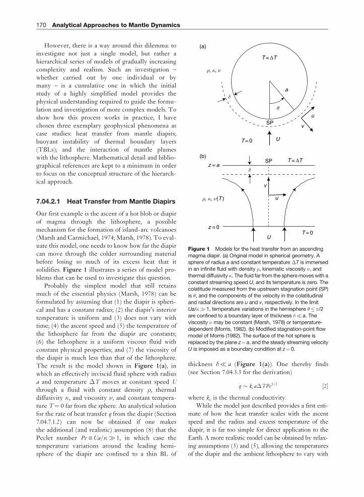
Our first example is the ascent of a hot blob or diapirof magma through the lithosphere, a possiblemechanism for the formation of island-arc volcanoes(Marsh and Carmichael, 1974; Marsh, 1978). To eval-uate this model, one needs to know how far the diapircan move through the colder surrounding materialbefore losing so much of its excess heat that itsolidifies. Figure 1 illustrates a series of model pro-blems that can be used to investigate this question.

Probably the simplest model that still retainsmuch of the essential physics (Marsh, 1978) can beformulated by assuming that (1) the diapir is spheri-cal and has a constant radius; (2) the diapir’s interiortemperature is uniform and (3) does not vary withtime; (4) the ascent speed and (5) the temperature ofthe lithosphere far from the diapir are constants;(6) the lithosphere is a uniform viscous fluid withconstant physical properties; and (7) the viscosity ofthe diapir is much less than that of the lithosphere.The result is the model shown in Figure 1(a), inwhich an effectively inviscid fluid sphere with radiusa and temperature �T moves at constant speed U

through a fluid with constant density �, thermaldiffusivity �, and viscosity �, and constant tempera-ture T¼ 0 far from the sphere. An analytical solutionfor the rate of heat transfer q from the diapir (Section7.04.7.1.2) can now be obtained if one makesthe additional (and realistic) assumption (8) that thePeclet number Pe XUa/�� 1, in which case thetemperature variations around the leading hemi-sphere of the diapir are confined to a thin BL of

thickness �� a (Figure 1(a)). One thereby finds(see Section 7.04.3.3 for the derivation)

q � kca�TPe1=2 ½2�

where kc is the thermal conductivity.While the model just described provides a first esti-

mate of how the heat transfer scales with the ascentspeed and the radius and excess temperature of thediapir, it is far too simple for direct application to theEarth. A more realistic model can be obtained by relax-ing assumptions (3) and (5), allowing the temperaturesof the diapir and the ambient lithosphere to vary with

(b)SP

SP

T = ΔT

T = ΔT

T = 0

T = 0

(a)

U

v

v

θ

δa

u

u

z = 0

z = a

U

δ

ρ, κ, ν (T )

ρ, κ, ν

Figure 1 Models for the heat transfer from an ascending

magma diapir. (a) Original model in spherical geometry. A

sphere of radius a and constant temperature �T is immersedin an infinite fluid with density �, kinematic viscosity �, and

thermal diffusivity�. The fluid far from the sphere moves with a

constant streaming speed U, and its temperature is zero. The

colatitude measured from the upstream stagnation point (SP)is �, and the components of the velocity in the colatitudinal

and radial directions are u and v, respectively. In the limit

Ua/�� 1, temperature variations in the hemisphere ��/2are confined to a boundary layer of thickness �� a. The

viscosity � may be constant (Marsh, 1978) or temperature-

dependent (Morris, 1982). (b) Modified stagnation-point flow

model of Morris (1982). The surface of the hot sphere isreplaced by the plane z¼ a, and the steady streaming velocity

U is imposed as a boundary condition at z¼0.


time. If these variations are slow enough, the heat trans-fer at each instant will be described by a law of the form[2], but with a time-dependent excess temperature�T(t). A model of this type was proposed by Marsh(1978), who obtained a solution in the form of a con-volution integral for the evolving temperature of adiapir ascending through a lithosphere with a prescribedfar-field temperature Tlith(t).

A different extension of the simple model ofFigure 1(a), also suggested by Marsh (1978), beginsfrom the observation that the viscosity of mantle mate-rials decreases strongly with increasing temperature. Ahot diapir will therefore be surrounded by a thin halo ofsoftened lithosphere, which will act as a lubricant andincrease the diapir’s ascent speed. The effectiveness ofthis mechanism depends on whether the halo is thickenough, and/or has a viscosity low enough, to carry asubstantial fraction of the volume flux ��a2U that thesphere must displace in order to move. Formally, thismodel is obtained by replacing the constant viscosity �in figure 1(a) by one that depends exponentially ontemperature as �¼ �0 exp(�T/�Tr).

While this new variable-viscosity model is morerealistic and dynamically richer than the originalmodel, its spherical geometry makes analytical solu-tion impossible except in certain limiting cases(Morris, 1982; Ansari and Morris, 1985). However,closer examination reveals that the spherical geome-try is not in fact essential: all that matters is that theflow outside the softened halo varies over a charac-teristic length scale a that greatly exceeds the halothickness. This recognition led Morris (1982) tostudy a simpler model in which the flow around thesphere is replaced by a stagnation-point flowbetween two planar boundaries z¼ 0 and z¼ a

(Figure 1(b)). The model equations now admit 1-Dsolutions T¼T(z) and �¼ �(z) for the temperatureand the vertical velocity, respectively, which can bedetermined using the method of matched asymptoticexpansions (MMAE) (Section 7.04.7.2) in the limit oflarge viscosity contrast �T/�Tr� 1 (Morris, 1982).

7.04.2.2 Plume Formation in TBLs

Our second example (Figure 2) is the formation ofplumes via the gravitational instability of a horizontalTBL. The first step in formulating a model for thisprocess is to choose a simple representation for therelevant physical properties (density, viscosity, andthermal diffusivity) of the fluid. Because these dependon pressure, temperature, and (possibly) chemical com-position, they will vary continuously with depth in the

TBL and with time (due to thermal diffusion). As a firstapproximation, however, one can model the depth dis-tribution of the fluid properties as a nondiffusing andspatially discontinuous two-fluid configuration in whicha dense layer with constant thickness h0, density�0þ��, and viscosity �1 overlies a half-space withdensity �0 and viscosity �0 (Figure 2(a)). The case of aless-dense BL beneath a denser fluid is obtained byturning the system upside down and switching the signof ��. Because both configurations are gravitationallyunstable, any small perturbation of the interfacebetween the two fluids will grow with time via theRayleigh–Taylor (R–T) instability. The growth rate ofan infinitesimal sinusoidal perturbation with arbitrarywave number k can be determined analytically (Selig,1965; Whitehead and Luther, 1975) via a standard linearstability analysis (Section 7.04.9.1).

While the simple RT model embodies some of theessential physics of plume formation, it is unable todescribe such crucial features as the characteristicperiodicity of TBL instabilities (Howard, 1964). Forthis purpose, a more realistic model that incorporatesa diffusing temperature field is required. Figure 2(b)shows such a model (Canright, 1987; Lemery et al.,

(a)

(b)

{

T = –ΔT

T = 0

z

h0

hx3

η(x3)

g

g

z = 0

x3 = 0

ρ0 + Δρ , η 1

ρ0(1 – g α T ),

ρ0, η0

ρ0, η0

W

U

ζ

û

^

Figure 2 Models for plume formation in a dense/coldthermal boundary layer. (a) Rayleigh–Taylor instability of a

layer of fluid with density �0þ�� and viscosity �1 above a

half-space of fluid with density �0 and viscosity �0. The initial

thickness of the dense layer is h0, and the deformation of theinterface is . The maximum values of the horizontal and

vertical velocities at the interface z¼ are U and W,

respectively, and u is the magnitude of the change inhorizontal velocity across the layer. (b) Buoyant instability of

a cold thermal boundary layer. The upper surface x3¼ 0 of a

fluid half-space is held at a fixed temperature ��T relative

to the interior. The density of the fluid varies withtemperature as �¼ �0(1�gT), where is the thermal

expansion coefficient. The thickness of the boundary layer

is h(x1, x2, t) and the viscosity within it is �(x3).


2000), in which a diffusive TBL grows away from acold surface and subsequently becomes unstable. Thedensity of the fluid varies linearly with temperature,and the viscosity � can vary as a function of the depthx3 within the TBL. The additional assumptions thatthe wavelength of the instability greatly exceeds thethickness of the TBL and that the horizontal compo-nents of the fluid velocity are constant across it thenpermit an analytical reduction of the full 3-D equa-tions to an equivalent set of 2-D equations for thehorizontal velocities and the first moment of thetemperature in the TBL (Section 7.04.8.3).

7.04.2.3 Plume–Lithosphere Interaction

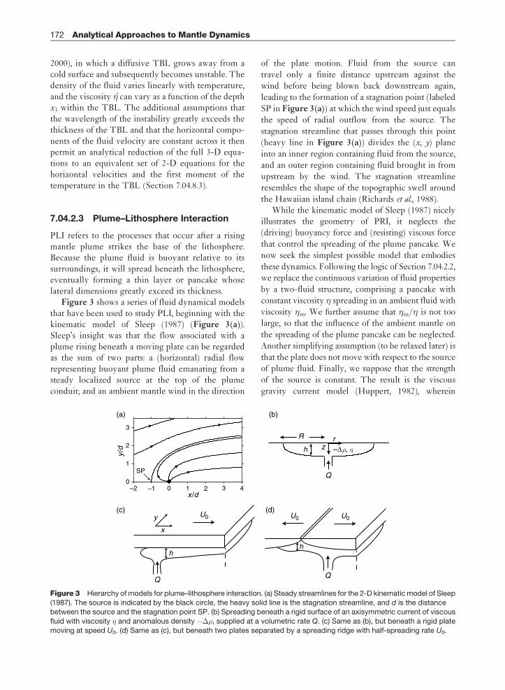
PLI refers to the processes that occur after a risingmantle plume strikes the base of the lithosphere.Because the plume fluid is buoyant relative to itssurroundings, it will spread beneath the lithosphere,eventually forming a thin layer or pancake whoselateral dimensions greatly exceed its thickness.

Figure 3 shows a series of fluid dynamical modelsthat have been used to study PLI, beginning with thekinematic model of Sleep (1987) (Figure 3(a)).Sleep’s insight was that the flow associated with aplume rising beneath a moving plate can be regardedas the sum of two parts: a (horizontal) radial flowrepresenting buoyant plume fluid emanating from asteady localized source at the top of the plumeconduit; and an ambient mantle wind in the direction

of the plate motion. Fluid from the source can

travel only a finite distance upstream against thewind before being blown back downstream again,

leading to the formation of a stagnation point (labeled

SP in Figure 3(a)) at which the wind speed just equals

the speed of radial outflow from the source. Thestagnation streamline that passes through this point

(heavy line in Figure 3(a)) divides the (x, y) plane

into an inner region containing fluid from the source,

and an outer region containing fluid brought in fromupstream by the wind. The stagnation streamline

resembles the shape of the topographic swell around

the Hawaiian island chain (Richards et al., 1988).While the kinematic model of Sleep (1987) nicely

illustrates the geometry of PRI, it neglects the(driving) buoyancy force and (resisting) viscous force

that control the spreading of the plume pancake. We

now seek the simplest possible model that embodies

these dynamics. Following the logic of Section 7.04.2.2,we replace the continuous variation of fluid properties

by a two-fluid structure, comprising a pancake with

constant viscosity � spreading in an ambient fluid with

viscosity �m. We further assume that �m/� is not toolarge, so that the influence of the ambient mantle on

the spreading of the plume pancake can be neglected.

Another simplifying assumption (to be relaxed later) is

that the plate does not move with respect to the sourceof plume fluid. Finally, we suppose that the strength

of the source is constant. The result is the viscous

gravity current model (Huppert, 1982), wherein

(c) (d)

(b)

0

1

2

3

–2 –1 0 1 2 3 4

(a)

SPQ

Q

rR

Q

U0U0U0

zh

y

x

x /d

y /d

hh

–Δ ρ, η

Figure 3 Hierarchy of models for plume–lithosphere interaction. (a) Steady streamlines for the 2-D kinematic model of Sleep

(1987). The source is indicated by the black circle, the heavy solid line is the stagnation streamline, and d is the distancebetween the source and the stagnation point SP. (b) Spreading beneath a rigid surface of an axisymmetric current of viscous

fluid with viscosity � and anomalous density ��, supplied at a volumetric rate Q. (c) Same as (b), but beneath a rigid plate

moving at speed U0. (d) Same as (c), but beneath two plates separated by a spreading ridge with half-spreading rate U0.


fluid with viscosity � and anomalous density ��relative to its surroundings is supplied at aconstant volumetric rate Q and spreads beneath astationary rigid surface (Figure 3(b)). The analyticalsolution for the closely related problem of acurrent with constant volume V is discussed inSection 7.04.8.1.

The next step is to generalize the gravity currentmodel by allowing the plate to move with a constantvelocity U0 relative to the source (Olson, 1990). Theresulting refracted plume model (Figure 3(c)) is inessence a dynamically self-consistent extension ofthe 2-D kinematic model of Sleep (1987), and isdiscussed further in Section 7.04.8.2.

As a final illustration, Figure 3(d) shows a furtherextension of the refracted plume model in which theuniform plate is replaced by two plates separated bya spreading ridge. Despite the increased complexity ofthis plume–ridge interaction model, analytical meth-ods can still profitably be applied to it (Ribe et al.,1995).

7.04.3 Dimensional and ScalingAnalysis

The goal of studying model problems in fluidmechanics is typically to determine functional rela-tions, or scaling laws, that obtain between certainparameters of interest and the various other para-meters on which they depend. Two simple yetpowerful methods that can be used for this purposeare dimensional analysis and scaling analysis.

7.04.3.1 Buckingham’s �-Theorem andDynamical Similarity

Dimensional analysis begins from the principle that thevalidity of physical laws cannot depend on the units inwhich they are expressed. An important consequence ofthis principle is the �-theorem of Buckingham (1914).

Suppose that there exists a (generally unknown)functional relationship among N-dimensional para-meters P1 P2, . . ., PN, such that

f1 P1; P2; . . . ; PNð Þ ¼ 0 ½3�

Let M < N be the number of the parameters Pn whichhave independent physical dimensions (note that adimensionally consistent functional relationshipamong the parameters Pn is impossible if M¼N ). Inmost (but not all!) cases, M is just the number of

independent units that enter into the problem, forexample, M¼ 3 for mechanical problems involvingunits of m, kg, and s and M¼ 4 for thermomechanicalproblems involving temperature (units K) in addi-tion. The �-theorem states that the functionalrelationship [3] is equivalent to a relation of the form

f2 �1; �2; . . . ; �N –Mð Þ ¼ 0 ½4�

where �1, �2, . . . , �N�M are N�M independentdimensionless combinations (or groups) of thedimensional parameters Pn. The fact that all systemsof units (SI, cgs, etc.) are equivalent requires that eachdimensionless group �i be a product of powers of thedimensional parameters Pn; no other functional formpreserves the value of the dimensionless group whenthe system of units is changed. The function f2, bycontrast, can have any form. While the total numberof independent groups �i is fixed (XN�M), thedefinitions of the individual groups are arbitraryand can be chosen as convenient. A more detaileddiscussion and proof of the �-theorem can be foundin Barenblatt (1996, chapter 1).

The �-theorem is the basis for the concept ofdynamical similarity, according to which two physicalsystems behave similarly (i.e., proportionally) if theyhave the same values of the dimensionless groups �i

that define them. The crucial point is that two systemsmay have identical values of �i even though they areof very different size, that is, even if the values of thedimensional parameters Pn are very different.Dynamical similarity is thus a natural generalizationof the concept of geometrical similarity, whereby, forexample, two triangles of different sizes are similar ifthey have the same values of the dimensionless para-meters (angles and ratios of sides) that define them.Geometrical similarity is a necessary, but not a suffi-cient, condition for dynamical similarity.

The importance of dynamical similarity for phy-sical modeling is that it allows results obtained in thelaboratory or on a computer to be applied to anothersystem with very different scales of length, time, etc.Its power derives from the fact that the function f2 in[4] has M fewer arguments than the original functionf1. Thus, an experimentalist or numerical analyst whoseeks to determine how a target dimensional para-meter P1 depends on the other N� 1 parametersneed not vary all of the latter individually; it sufficesto vary only N�M� 1 dimensionless parameters.Consequently, if the variation of a given dimensionalparameter requires 10 samplings, then use of the�-theorem reduces the effort involved in searching


the parameter space by a factor 10M (Barenblatt,1996; see also Chapter 7.02) By the same token, the�-theorem makes possible a far more economicalrepresentation of experimental or numerical data. Asan example, suppose that we have N¼ 5 dimensionalparameters P1–P5 from which N�M¼ 2 indepen-dent dimensionless groups �1 and �2 can beformed. To represent our data without the help ofthe �-theorem, we would need many shelves (onefor each value of P5), each containing many books(one for each value of P4), each containing manypages (one for each value of P3), each containing aplot of P2 versus P1. By using the �-theorem, how-ever, we can collapse the whole library onto a singleplot of �2 versus �1.

As a simple illustration of the �-theorem, consideragain the model for heat transfer from a hot sphere(Figure 1(a)). Suppose that we wish to determine theradial temperature gradient � (proportional to the localconductive heat flux) as a function of position on thesphere’s surface. A list of all the relevant parametersincludes the following eight (units in parentheses):�(K m�1), a(m), U(m s�1), �(kg m�3), �(m2 s�1),�(m2 s�1), �T(K), and � (dimensionless). However, �can be eliminated immediately because it is the onlyparameter that involves units of mass: no dimensionlessgroup containing it can be defined. The remainingparameters are N¼ 7 in number, M¼ 3 of which (e.g.,a, �T, and U ) have independent units, so N�M¼ 4independent dimensionless groups can be formed. It isusually good practice to start by defining a single groupcontaining the target parameter (� here.) While inspec-tion usually suffices, one can also proceed moreformally by writing the group (�1 say) as a product ofthe desired parameter (�) and unknown powers of anyset of M parameters with independent dimensions, forexample, �1¼ �an1�T n2U n3. The requirement that �1

be dimensionless then implies n1¼ 1, n2¼�1, andn3¼ 0. Additional groups are then obtained by applyingthe same procedure to the remaining dimensional para-meters in the list (� and � in this case.) Finally, anyremaining parameters in the list that are already dimen-sionless (� in this case) can be used as groups bythemselves. For the hot sphere, the result is

�a

�T¼ fct

Ua

�;

Ua

�; �

� �½5�

where fct is an unknown function. The groupsUa/� X Pe, Ua/� X Re, and �a/�T X N are tradition-ally called the Peclet number, the Reynolds number,and the (local) Nusselt number, respectively (the last

to be distinguished from the global Nusselt numberNu X

Rs

N dS that measures the total heat flux acrossthe sphere’s surface S.) As we remarked earlier, thedefinitions of the dimensionless groups in a relationlike [5] are not unique. Thus one can replace anygroup by the product of itself and arbitrary powers ofthe other groups, for example, Pe in [5] by the Prandtlnumber �/� X Pe/Re. Furthermore, it often (but notalways!) happens that the target parameter ceases todepend on a dimensionless group whose value is verylarge or very small. For example, in a very viscousfluid such as the mantle, Re << 1 because inertia isnegligible, and so Re no longer appears as an argu-ment in [5].

7.04.3.2 Nondimensionalization

When the equations governing the dynamics of theproblem at hand are known, another method ofdimensional analysis becomes available: nondimen-sionalization. We illustrate this using the sameexample of a hot sphere.

The first step is to write down the governingequations, together with all the relevant initial andboundary conditions. Because the problem is bothsteady and axisymmetric, the dependent variablesare the temperature T(r, �) and the velocity u(r, �),where r and � are the usual spherical coordinates. Ifviscous dissipation is negligible, the governing equa-tions and boundary conditions are (see Chapter 7.06)

� ? u ¼ 0; u ? �T ¼ �r2T ;u ? �u ¼ – � – 1�p þ �r2u

½6a�

T a; �ð Þ –�T ¼T 1; �ð Þ ¼ u a; �ð Þ¼ u 1; �ð Þ –Uez ¼ 0 ½6b�

where ez is a unit vector in the direction of the steadystream far from the sphere. The next step is to definedimensionless variables (denoted, e.g., by primes)using scales that appear in the equations and/or initialand boundary conditions. An obvious (but notunique) choice is r9¼ r/a, T9¼T/�T, u9¼ u/U,and p9¼ a(p� p0)/��U, where p0 is the (dynamicallyinsignificant) pressure far from the sphere.Substituting these definitions into [6] and immediatelydropping the primes to avoid notational overload, weobtain the dimensionless BVP:

� ? u ¼ 0; Pe u ? �T ¼ r2T ;Re u ? �u ¼ –�p þr2u

½7a�

T 1; �ð Þ–1¼ T 1; �ð Þ ¼ u 1; �ð Þ ¼ u 1; �ð Þ–ez ¼ 0 ½7b�


where Pe and Re are the Peclet and Reynolds num-bers defined in Section 7.04.3.1. Now because theseare the only dimensionless parameters appearing in[7a] and [7b], the dimensionless temperature musthave the form T¼T (r, �, Pe, Re). Differentiating thiswith respect to r and evaluating the result on thesurface r¼ 1 to obtain the quantity �a/�T, we findthe same result [5] as we did using the �-theorem.

Whether one chooses to do dimensional analysisusing the �-theorem or nondimensionalizationdepends on the problem at hand. The �-theorem isof course the only choice if the governing equationsare not known, but its effective use then requires agood intuition of what the relevant physical para-meters are. When the governing equations areknown, nondimensionalization is usually the bestchoice, as the relevant physical parameters appearexplicitly in the equations and initial/boundaryconditions.

7.04.3.3 Scaling Analysis

Except when N�M¼ 1, dimensional analysis yieldsa relation involving an unknown function of one ormore dimensionless arguments. To determine thefunctional dependence itself, methods that go beyonddimensional analysis are required. The most detailedinformation is provided by a full analytical or numer-ical solution of the problem, but finding suchsolutions is rarely easy. Scaling analysis is a powerfulintermediate method that provides more informationthan dimensional analysis while avoiding the labor ofa complete solution. It proceeds by estimating theorders of magnitude of the different terms in a set ofgoverning equations, using both known and unknownquantities, and then exploiting the fact that the termsmust balance (the definition of an equation!) to deter-mine how the unknown quantities depend on theknown.

To illustrate this, we consider once again theproblem of determining the local Nusselt numberN for the hot sphere, but now in the specific limitRe� 1 and Pe� 1. Recall that Re measures the ratioof advection to diffusion of gradients in velocity(Xvorticity), while Pe does the same for gradients intemperature. In the limit Re� 1, advection of velo-city gradients is negligible relative to diffusioneverywhere in the flow field, and u is given by theclassic Stokes–Hadamard solution for slow viscousflow around a sphere of another fluid (Section7.04.5.3.2). When Pe� 1, temperature gradients aretransported by advection with negligible diffusion

everywhere except in a thin TBL of thickness�(�)� a around the leading hemisphere whereadvection and diffusion are of the same order.Because radial temperature gradients greatly exceedsurface-tangential gradients within this layer, thetemperature distribution there is described by thesimplified BL forms of the continuity and energyequations (cf. Section 7.04.7)

a sin �vr þ u sin �ð Þ�¼ 0 ½8a�

a – 1uT� þ vTr ¼ �Trr ½8b�

where u(r, �) and v(r, �) are the tangential (�) andradial (r) components of the velocity, respectively,and subscripts indicate partial derivatives. Equations[8] are obtained from [145] by setting x¼ a� andr¼ a sin �.

We begin by determining the relative magnitudesof the velocity components u and v in the BL. Whilethese can be found directly from the Stokes–Hadamard solution, it is more instructive to do ascaling analysis of the continuity equation [8a].Now vr��v/�, where �v is the change in v acrossthe BL; but because v(a, �)¼ 0, �v¼ v. Similarly,u��u/��, where �u is the change in u over anangle �� of order unity from the forward stagnationpoint �¼ 0 toward the equator �¼ �/2. But becauseu(r, 0)¼ 0, �u¼ u. The continuity equation thereforeimplies

v � �=að Þu ½9�

We turn now to the left-hand side (LHS) of theenergy equation [8b], whose two terms representadvection of temperature gradients in the tangentialand radial directions, respectively. Now the radialtemperature gradient Tr��T/� greatly exceedsthe tangential gradient a�1T��T/a, but this dif-ference is compensated by the smallness of the radialvelocity v� (�/a)u, and so the terms representingtangential and radial advection are of the sameorder. The balance of advection and diffusion in theBL is therefore a�1uT��Tr r , which together withTrr��T/�2 implies

�2 � �a=u ½10�

It remains only to determine an expression for u,which depends on the ratio � of the viscosity of thesphere to that of the surrounding fluid. We considerthe limiting cases �� 1 (a traction-free sphere) and�� 1 (an effectively rigid sphere). Because the fluidoutside the sphere has constant viscosity, u variessmoothly over a length scale �a. Within the TBL,


therefore, u can be approximated by the first term ofits Taylor series expansion in the radial distancer� a X away from the sphere’s surface. If the sphereis traction free, uj¼0¼ 0, implying that u�U isconstant across the TBL to lowest order. If howeverthe sphere is rigid, uj¼0¼ 0 and u� (/a)U. Thetangential velocity u at the outer edge � � of theTBL is therefore

u � �=að ÞnU ½11�

where n¼ 0 for a traction-free sphere and n¼ 1 for arigid sphere. Substituting [11] into [10] and notingthat N � a/�, we obtain

N � Pe1=ðnþ2Þfn �ð Þ ½12�

where fn(�) (n¼ 1 or 2) are unknown functions. Thuswhen Pe� 1, N � Pe1/2 if the sphere is traction-freeand N � Pe1/3 if it is rigid. N is greater in the formercase because the tangential velocity u, which carriesthe heat away from the sphere, is �U across thewhole TBL.

7.04.4 Self-Similarity andIntermediate Asymptotics

In geophysics and in fluid dynamics more generally,one often encounters functions that exhibit the prop-erty of scale-invariance or self-similarity. As anillustration, consider a function f ( y, t) of two arbi-trary variables y and t. The function f is self-similar ifit has the form

f y; tð Þ ¼ G tð ÞF y

� tð Þ

� �½13�

where F, G, and � are arbitrary functions and� X y/�(t) is the similarity variable. Self-similaritysimply means that curves of f versus y for differentvalues of t can be obtained from a single universalcurve F(�) by stretching its abscissa and ordinate byfactors �(t) and G(t), respectively.

Self-similarity is closely connected with the con-cept of intermediate asympotics (Barenblatt, 1996). Inmany physical situations, one is interested in thebehavior of a system at intermediate times, longafter it has become insensitive to the details of theinitial conditions but long before it reaches a finalequilibrium state. The behavior of the system at theseintermediate times is often self-similar, as we nowillustrate using a simple example of conductive heattransfer (Barenblatt, 1996, Section 7.04.2.1).

7.04.4.1 Conductive Heat Transfer

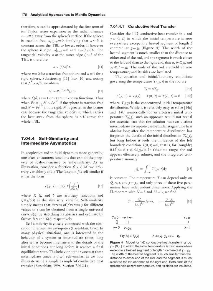
Consider the 1-D conductive heat transfer in a rod

y P [0, L] in which the initial temperature is zero

everywhere except in a heated segment of length h

centered at y¼ y0 (Figure 4). The width of the

heated segment is much smaller than the distance to

either end of the rod, and the segment is much closer

to the left end than to the right end, that is, h� y0 and

y0� L� y0. The ends of the rod are held at zero

temperature, and its sides are insulated.The equation and initial/boundary conditions

governing the temperature T ( y, t) in the rod are

Tt ¼ �Tyy ½14a�

T y; 0ð Þ ¼ T0ðyÞ; Tð0; tÞ ¼ T L; tð Þ ¼ 0 ½14b�

where T0( y) is the concentrated initial temperaturedistribution. While it is relatively easy to solve [14a]and [14b] numerically for an arbitrary initial tem-perature T0( y), such an approach would not revealthe essential fact that the solution has two distinctintermediate asymptotic, self-similar stages. The firstobtains long after the temperature distribution hasforgotten the details of the initial distribution T0( y),but long before it feels the influence of the leftboundary condition T(0, t)¼ 0, that is, for (roughly)0.1h2/�� t � 0.1y0

2/�. In this time range, the rodappears effectively infinite, and the integrated tem-perature anomaly

Q ¼Z 1–1

T y; tð Þdy ½15�

is constant. The temperature T can depend only onQ, �, t, and y� y0, and only three of these five para-meters have independent dimensions. Applying the�-theorem with N¼ 5 and M¼ 3, we find

T ¼ Q

�tð Þ1=2F1 �ð Þ; � ¼ y – y0

�tð Þ1=2½16�

T = 0 T = 0h

y = 0 y = Ly = y0

T (y, 0) = T0(y ) h << y0, y0 << L – y0

Figure 4 Model for 1-D conductive heat transfer in a rody P [0, L] in which the initial temperature is zero everywhere

except in a heated segment of length h centered at y¼ y0.

The width of the heated segment is much smaller than thedistance to either end of the rod, and the segment is much

closer to the left end than to the right end. Both ends of the

rod are held at zero temperature, and its sides are insulated.


which is of the general self-similar form [13].Substituting [16] into [14a] and [15], we find that F1

satisfies

2F 01 þ �F 91 þ F1 ¼ 0;

Z 1–1

F1 d� ¼ 1 ½17�

Upon solving [17] subject to F1(1)¼ 0, [16]becomes

T ¼ Q

2ffiffiffiffiffiffiffiffi��tp exp –

y – y0ð Þ2

4�t

� �½18�

The second intermediate asymptotic stage occurslong after the temperature distribution has begun tobe influenced by the left boundary conditionT(0, t)¼ 0, but long before the influence of theright boundary condition T(L, t)¼ 0 is felt, ory0

2/�� t� 0.1(L� y0)2/�. During this time interval,the rod is effectively semi-infinite, and the tempera-ture satisfies the boundary conditions

T 0; tð Þ ¼ T 1; tð Þ ¼ 0 ½19�

The essential step in determining the similarity solu-tion is to identify a conserved quantity. Multiplying[14a] by y, integrating from y¼ 0 to y¼1, and thentaking the time derivative outside the integral sign,we obtain

d

dt

Z 10

yT dy ¼ �Z 1

0

yTyydy ½20�

However, the RHS of [20] is zero, as can be shown byintegrating by parts, applying the conditions [19],and noting that yTyjy¼1¼ 0 because Ty! 0 morerapidly (typically exponentially) than y!1. Thetemperature moment

M ¼Z 1

0

yT dy ½21�

is therefore constant; and because the initial tempera-ture distribution is effectively a delta-functionconcentrated at y¼ y0, M¼Q y0. Now in the timeinterval in question, the influence of the temperaturedistribution that existed at the time 0.1y0

2/� whenthe heated region first reached the near end y¼ 0 ofthe rod will no longer be felt. The temperature willtherefore no longer depend on y0, but only on M, �, y,and t� t0, where t0 is the effective starting time forthe second stage, to be determined later. Applyingthe �-theorem as before, we find

T ¼ M

� t – t0ð Þ F2 �ð Þ; � ¼ yffiffiffiffiffiffiffiffiffiffiffiffiffiffiffiffi� t – t0ð Þ

p ½22�

Now substitute [22] into [14a] and [21], and solve theresulting equations subject to F2(0)¼ F2(1)¼ 0,whereupon [22] becomes

T ¼ My

2ffiffiffi�p

� t – t0ð Þ½ �3=2exp –

y2

4� t – t0ð Þ

� �½23�

The final step is to determine the starting timet0¼�y0

2/6� (Barenblatt, 1996, p. 74). Because t0 < 0,that is, before the rod was originally heated, it repre-sents a virtual starting time with respect to which thebehavior of the second stage is self-similar.

7.04.4.2 Classification of Self-SimilarSolutions

The solutions [18] and [23] are examples of whatBarenblatt (1996) calls self-similar solutions of thefirst kind, for which dimensional analysis (in somecases supplemented by scaling analysis of the govern-ing equations) suffices to find the similarity variable.They are distinguished from self-similar solutions ofthe second kind, for which the similarity variable canonly be found by solving an eigenvalue problem. Wewill meet some examples of these below, in thesections on viscous eddies in a corner (Section7.04.5.3.4) and the spreading of viscous gravitycurrents (Section 7.04.8.1).

An example of a self-similar solution that does notfit naturally into either class is the impulsive coolingof a half-space deforming in pure shear. Suppose thatthe half-space y� 0 has temperature T¼ 0 initially,and that at time t¼ 0 the temperature at its surfacey¼ 0 is suddenly decreased by an amount �T. The2-D velocity field in the half-space is u¼ _ (xex�yey), where _ is the constant rate of extension of thesurface y¼ 0 and ex and ey are unit vectors parallel toand normal to the surface, respectively. Given thisvelocity field, a temperature field T¼T( y, t) that isindependent of the lateral coordinate x is an allow-able solution of the governing advection–diffusionequation Ttþ u ? �T¼�r2T, which takes the form

Tt – _ yTy ¼ �Tyy ½24�

subject to the conditions Tðy; 0Þ ¼ T ð1; tÞ ¼T ð0; tÞ þ�T ¼ 0. The limit _ ¼ 0 corresponds to

the classic problem of the impulsive cooling of astatic half-space.

Neither dimensional analysis nor scaling analysis issufficient to determine the similarity variable, whichdoes not have the standard power-law monomial form.However, the solution can be found via a generalized


form of the familiar separation-of-variables procedureoften used to solve PDEs such as Laplace’s equation.Note first that the amplitude �T of the temperaturein the half-space is a constant. This implies that thefunction G(t) in the similarity transformation [13] mustbe independent of time, whence T(y, t)¼�TF(y/�(t)).Substituting this expression into [24] and bringing allterms involving �(t) to the LHS, we obtain

� _� þ _ ��

¼ –F 0

�F 9½25�

where dots and primes denote differentiation withrespect to t and � X y/�(t), respectively. Now theLHS of [25] is a function of t only, whereas theRHS depends on y through the similarity variable �.Equation [25] is therefore consistent only if bothsides are equal to a constant �2, which is positivebecause _�> 0. The solutions for � and F subject tothe conditions �(0)¼ F(1)¼ F(0)� 1¼ 0 are

F ¼ erfc�yffiffiffi2p�; � ¼ � �

_ 1 – exp – 2 _ tð Þ½ �

n o1=2

½26�

Evidently � cancels out when the solution for � issubstituted into the solution for F, because differentvalues of � merely correspond to different (arbitrary)definitions of the thermal layer thickness �. With _ ¼ 0and the conventional choice � ¼

ffiffiffi2p

, we recover thewell-known solution � ¼ 2

ffiffiffiffiffi�tp

for a static half-space.However, when _ > 0, the BL thickness approaches asteady-state value �¼ (2�/ _ )1/2 for which the down-ward diffusion of temperature gradients is balanced byupward advection, and the similarity variable involvesan exponential function of time. The only reliable wayto find such nonstandard self-similar solutions is theseparation-of-variables procedure outlined above. Butthe same procedure works just as well for problemswith similarity variables of standard form, and there-fore will be used throughout this chapter.

In conclusion, we note that similarity transforma-tions can also be powerful tools for reducing andinterpreting the output of numerical models. As asimple example, suppose that some such model yieldsvalues of a dimensionless parameter W as a functionof two dimensionless groups �1 and �2. Dependingon the physics of the problem, it may be possible toexpress the results in the self-similar form

W �1; �2ð Þ ¼ F1 �1ð ÞF2�1

F3 �2ð Þ

� �½27�

where F1–F3 are functions to be determined numeri-cally. A representation of the form [27] is not

guaranteed to exist, but when it does it provides acompact way of representing multidimensionalnumerical data by functions of a single variable thatcan be fit by simple analytical expressions. An exam-ple of the use of this technique for a probleminvolving five dimensionless groups is the lubricationtheory model for plume–ridge interaction of Ribeand Delattre (1998).

7.04.4.3 Intermediate Asymptotics withRespect to Parameters: The R–T Instability

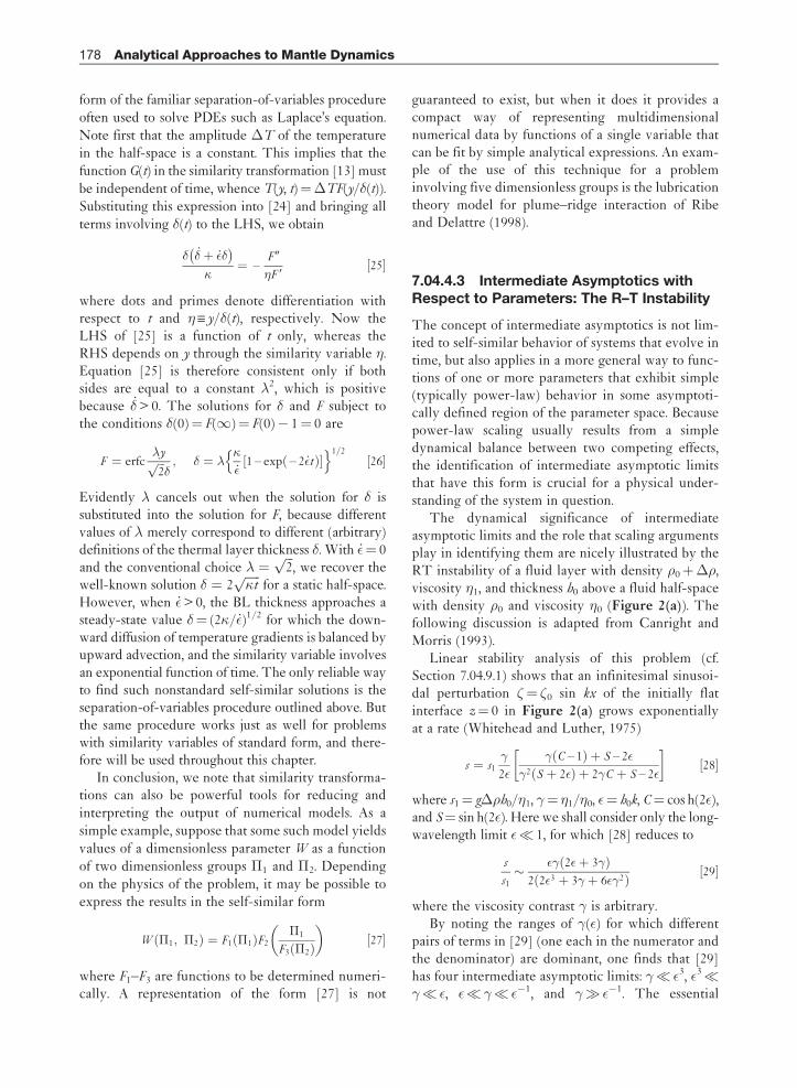
The concept of intermediate asymptotics is not lim-ited to self-similar behavior of systems that evolve intime, but also applies in a more general way to func-tions of one or more parameters that exhibit simple(typically power-law) behavior in some asymptoti-cally defined region of the parameter space. Becausepower-law scaling usually results from a simpledynamical balance between two competing effects,the identification of intermediate asymptotic limitsthat have this form is crucial for a physical under-standing of the system in question.

The dynamical significance of intermediateasymptotic limits and the role that scaling argumentsplay in identifying them are nicely illustrated by theRT instability of a fluid layer with density �0þ��,viscosity �1, and thickness h0 above a fluid half-spacewith density �0 and viscosity �0 (Figure 2(a)). Thefollowing discussion is adapted from Canright andMorris (1993).

Linear stability analysis of this problem (cf.Section 7.04.9.1) shows that an infinitesimal sinusoi-dal perturbation ¼ 0 sin kx of the initially flatinterface z¼ 0 in Figure 2(a) grows exponentiallyat a rate (Whitehead and Luther, 1975)

s ¼ s1�

2

� C – 1ð Þ þ S – 2

�2 S þ 2 ð Þ þ 2�C þ S – 2

� �½28�

where s1¼ g��h0/�1, �¼ �1/�0, ¼ h0k, C¼ cos h(2 ),and S¼ sin h(2 ). Here we shall consider only the long-wavelength limit � 1, for which [28] reduces to

s

s1� � 2 þ 3�ð Þ

2 2 3 þ 3� þ 6 �2ð Þ ½29�

where the viscosity contrast � is arbitrary.By noting the ranges of �( ) for which different

pairs of terms in [29] (one each in the numerator andthe denominator) are dominant, one finds that [29]has four intermediate asymptotic limits: �� 3, 3�� , � �� 1, and �� 1. The essential


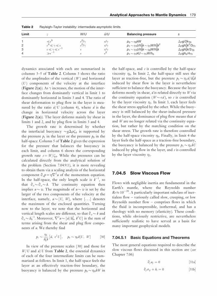
dynamics associated with each are summarized incolumns 3–5 of Table 2. Column 3 shows the ratioof the amplitudes of the vertical (W ) and horizontal(U ) components of the velocity at the interface(Figure 2(a)). As � increases, the motion of the inter-face changes from dominantly vertical in limit 1 todominantly horizontal in limits 3 and 4. The ratio ofshear deformation to plug flow in the layer is mea-sured by the ratio u/U (column 4), where u is thechange in horizontal velocity across the layer(Figure 2(a)). The layer deforms mainly by shear inlimits 1 and 2, and by plug flow in limits 3 and 4.

The growth rate is determined by whetherthe interfacial buoyancy �g��0 is supported bythe pressure p1 in the layer or the pressure p0 in thehalf-space. Column 5 of Table 2 gives the expressionfor the pressure that balances the buoyancy ineach limit, and column 6 shows the correspondinggrowth rate s¼W/0. While the pressures can becalculated directly from the analytical solution ofthe problem (Section 7.04.9.1), it is more revealingto obtain them via a scaling analysis of the horizontalcomponent qxp¼ �r2u of the momentum equation.In the half-space, the only length scale is k�1, sothat qx� qz� k. The continuity equation thenimplies u�w. The magnitude of u�w is set by thelarger of the two components of the velocity at theinterface, namely, u� [U, W], where [. . .] denotesthe maximum of the enclosed quantities. Turningnow to the layer, we note that the horizontal andvertical length scales are different, so that qx� k andqz� h0

�1. Moreover, r2u� [u/h02, k2U] is the sum of

terms arising from the shear and plug flow compo-nents of u. We thereby find

p1 ��1

h20k

u; 2U

; p0 � �0k U ; W½ � ½30�

In view of the pressure scales [30] and those forW/U and u/U from Table 2, the essential dynamicsof each of the four intermediate limits can be sum-marized as follows. In limit 1, the half-space feels thelayer as an effectively traction-free boundary, thebuoyancy is balanced by the pressure p0� �0kW in

the half-space, and s is controlled by the half-spaceviscosity �0. In limit 2, the half-space still sees thelayer as traction-free, but the pressure p1� �1u/h0

2k

induced by shear flow in the layer is neverthelesssufficient to balance the buoyancy. Because the layerdeforms mostly in shear, u is related directly to W viathe continuity equation (W� u ), so s is controlledby the layer viscosity �1. In limit 3, each layer feelsthe shear stress applied by the other. While the buoy-ancy is still balanced by the shear-induced pressurein the layer, the dominance of plug flow means that u

and W are no longer related via the continuity equa-tion, but rather by the matching condition on theshear stress. The growth rate is therefore controlledby the half-space viscosity �0. Finally, in limit 4 thelayer feels the half-space as a traction-free boundary,the buoyancy is balanced by the pressure p1� �1kU

induced by plug flow in the layer, and s is controlledby the layer viscosity �1.

7.04.5 Slow Viscous Flow

Flows with negligible inertia are fundamental in theEarth’s mantle, where the Reynolds numberRe 10�20. A particularly important subclass of iner-tialess flow – variously called slow, creeping, or lowReynolds number flow – comprises flows in whichthe fluid is incompressible, isothermal, and has arheology with no memory (elasticity). These condi-tions, while obviously restrictive, are neverthelesssufficiently realistic to have served as a basis formany important geophysical models.

7.04.5.1 Basic Equations and Theorems

The most general equations required to describe theslow viscous flows discussed in this section are (seeChapter 7.06)

qj uj ¼ 0 ½31a�

qj�ij þ bi ¼ 0 ½31b�

Table 2 Rayleigh–Taylor instability: intermediate asymptotic limits

Limit g W/U u/U Balancing pressure s

1 � 3 2/� /� p0� �0kW ��g/2k�0

2 3� �� 2/� /� p1� �1u/h02k� �1W/h0

3k2 ��gh03k2/3�1

3 � �� 1 /� p1� �1u/h02k� �0W/h0

2k ��gh02k/2�0

4 � �1 2 p1� �1kU� �1W/h0 ��gh0/4�1


bi ¼ – �qi� ½31c�

r2� ¼ 4�G� ½31d�

�ij ¼ – p þ 2�eij ; eij ¼1

2qi uj þ qj ui

� �½31e�

� ¼ �0 I=I0ð Þ – 1þ1=n; I ¼ eij eij

� �1=2 ½31f �

where ui is the velocity vector, �ij is the stress tensor, bi

is the gravitational body force per unit volume, � is thegravitational potential, � is the density, p is the pressure,� is the viscosity, and eij is the strain-rate tensor withsecond invariant I. Equation [31a] is the incompressi-bility condition. Equation [31b] expresses conservationof momentum in the absence of inertia, and states thatthe net force (viscous plus gravitational) acting on eachfluid element is zero. Equation [31d] is Poisson’s equa-tion for the gravitational potential. Equation [31e] is thestandard constitutive relation for a viscous fluid.Finally, [31f] is the strain-rate-dependent viscosityfor a power-law fluid (sometimes called a generalizedNewtonian fluid), where �0 is the viscosity at a refer-ence strain rate I¼ I0 and n is the power-law exponent.A Newtonian fluid has n¼ 1, while the rheology of dryolivine deforming by dislocation creep is welldescribed by [31f] with n 3.5 (Bai et al., 1991). Adiscussion of more complicated non-Newtonian fluidsis beyond the scope of this chapter; the interestedreader is referred to Bird et al. (1987).

Viscous flow described by [31] can be driveneither externally, by velocities and/or stresses

imposed at the boundaries of the flow domain, or

internally, by buoyancy forces (internal loads) arising

from lateral variations of the density �. On the scale

of the whole mantle, the influence of long-wave-

length lateral variations of � on the gravitational

potential � (self-gravitation) is significant and cannot

be neglected. In modeling flow on smaller scales,

however, one generally ignores Poisson’s equation

[31d] and replaces �� in [31c] by a constant gravita-

tional acceleration �g.Slow viscous flow exhibits the property of instan-

taneity: ui and �ij at each instant are determined

throughout the fluid solely by the distribution of

forcing (internal loads and/or boundary motions)

acting at that instant. Instantaneity requires that the

fluid have no memory (elasticity) and that accelera-

tion and inertia be negligible; there is then no time

lag between the forcing and the fluid’s response to it.

A corollary is that slow viscous flow is quasi-static,

any time-dependence being due entirely to the time-

dependence of the forcing.

The theory of slow viscous flow is most highlydeveloped for the special case of Newtonian fluids(Stokes flow), and several excellent monographs onthe subject exist (Ladyzhenskaya, 1963; Langlois,1964; Happel and Brenner, 1991; Kim and Karrila,1991; Pozrikidis, 1992). Relative to general slowviscous flow, Stokes flow exhibits the important addi-tional properties of linearity and reversibility.Linearity implies that for a given geometry, a sumof different solutions (e.g., for different forcing dis-tributions) is also a solution. It also implies that ui and�ij are directly proportional to the forcing that gen-erates them, and hence for example, that the forceacting on a body in Stokes flow is proportional to itsspeed. Reversibility refers to the fact that changingthe sign of the forcing terms reverses the signs of ui

and �ij for all material particles. The reversibilityprinciple is especially powerful when used in con-junction with symmetry arguments. It implies, forexample, that a body with fore-aft symmetry fallingfreely in any orientation in Stokes flow experiencesno torque, and that the lateral separation of twospherical diapirs with different radii is the samebefore and after their interaction (Manga, 1997).

An important theorem concerning Stokes flow isthe ‘Lorentz reciprocal theorem,’ which relates twodifferent Stokes flows (ui, �ij, bi) and (ui

�, �ij�, bi�). This

theorem is the starting point for the boundary-inte-gral representation of Stokes flow derived in Section7.04.5.6.4. Consider the scalar quantity ui

�qj�ij , whichwe manipulate as follows:

u�i qj�ij ¼ qj u�i �ij

� �– �ij qj u�i

¼ qj u�i �ij

� �– – p�ij þ 2�eij

� �qj u�i

¼ qj u�i �ij

� �– 2�eij e

�ij ½32�

By subtracting from [32] the analogous expression withthe starred and unstarred fields interchanged and set-ting qj �ij¼�bi and qj �ij

�¼�bij�, we obtain the

differential form of the Lorentz reciprocal theorem:

qj u�i �ij – ui��ij

� �¼ uj b�j – u�j bj ½33�

An integral form of the reciprocal theorem isobtained by integrating [33] over a volume V

bounded by a surface S and applying the divergencetheorem, yielding

ZS

u�i �ij nj dS þZ

V

bj u�j dV ¼

ZS

ui��ij nj dS

þZ

V

b�j uj dV ½34�

where nj is the outward unit normal to S.


Two additional theorems for Stokes flow concernthe total rate of energy dissipation

E ¼ 2�

ZV

eij eij dV ½35�

in a volume V. The first states that the solution of theStokes equations subject to given boundary condi-tions is unique, and is most easily proved by showingthat the energy dissipated by the difference of twosupposedly different solutions is zero (Kim andKarrila, 1991, p. 14.) The second is the minimumdissipation theorem, which states that a solution ofthe Stokes equations for given boundary conditionsdissipates less energy than any other solenoidal vec-tor field satisfying the same boundary conditions(Kim and Karrila, 1991, p. 15.) Note that this theoremmerely compares a Stokes flow with other flows thatdo not satisfy the Stokes equations. It says nothingabout the relative rates of dissipation of Stokes flowswith different geometries and/or boundary condi-tions, and therefore its use as a principle ofselection among such flows is not justified.

7.04.5.2 Potential Representations forIncompressible Flow

In an incompressible flow satisfying � ? u¼ 0, onlyN� 1 of the velocity components ui are independent,where N¼ 3 in general and N¼ 2 for 2-D andaxisymmetric flows. This fact allows one to expressall the velocity components in terms of derivatives ofN� 1 independent scalar potentials, thereby redu-cing the number of independent variables in thegoverning equations. The most commonly usedpotentials are the streamfunction (for N¼ 2) andthe poloidal potential P and the toroidal potential T(for N¼ 3). Below we give expressions for thecomponents of u in terms of these potentials inCartesian (x, y, z), cylindrical (�, �, z), and spherical(r, �, �) coordinates, together with the PDEs theysatisfy for the important special case of constantviscosity.

7.04.5.2.1 2-D and axisymmetric flows

A 2-D flow is one in which the velocity vector u iseverywhere perpendicular to a fixed direction (ez

say) in space. The velocity can then be representedin terms of a streamfunction by

u ¼ ez � � ¼ – ex y þ ey x ¼ – e� � þe�� ½36�

The PDE satisfied by is obtained by applying theoperator ez�� to the momentum equation [31b]with the constitutive law [31e]. If the viscosity isconstant and bi¼ 0, satisfies the biharmonicequation

r41 ¼ 0; r2

1 ¼ q2xx þ q2

yy ¼ �–1q� �q��

þ �–2q2�� ½37�

An axisymmetric flow (without swirl) is one inwhich u at any point lies in the plane containing the

point and some fixed axis (ez, say). For this case,

u ¼ e�� ¼ –

ez

� � þ

e�

� z ½38a�

u ¼ e�r sin�

� � ¼ e�r sin�

r –er

r 2sin� � ½38b�

where is referred to as the Stokes streamfunction.The PDE satisfied by the Stokes streamfunction isobtained by applying the operator e�� to themomentum equation. For a fluid with constant visc-osity and no body force, the result is

E4 ¼ 0;

E2 ¼ h3

h1h2

qqq1

h2

h1h3

qqq1

� �þ qqq2

h1

h2h3

qqq2

� �� ½39�

where (q1, q2) are orthogonal coordinates in any half-plane normal to e�, (h1, h2) are the correspondingscale factors, and h3 is the scale factor for theazimuthal coordinate �. Thus (q1, q2, h1, h2, h3)¼(z, �, 1, 1, �) in cylindrical coordinates and(q1; q2; h1; h2; h3Þ ¼ ðr ; �; 1; r ; r sin �Þ in sphericalcoordinates. The operator E 2 is in general differentfrom the Laplacian operator

r21 ¼

1

h1h2h3

qqq1

h2h3

h1

qqq1

� �þ qqq2

h1h3

h2

qqq2

� �� ½40�

the two being identical only for 2-D flows (h3¼ 1).

7.04.5.2.2 3-D flows

The most commonly used (but not the only) poten-

tial representation of 3-D flows in geophysics is a

decomposition of the velocity u into poloidal and

toroidal components (Backus, 1958; Chandrasekhar,

1981). This representation requires the choice of a

preferred direction, which is usually chosen to be an

upward vertical (ez) or radial (er) unit vector.

Relative to Cartesian coordinates, the poloidal/tor-

oidal decomposition has the form

u ¼ �� ez � �Pð Þ þ ez � �T¼ ex – P xz – T y

� �þ ey – P yz þ T x

� �þ ezr2

1P ½41�


where P is the poloidal potential and T is thetoroidal potential. The associated vorticityw X�� u is

w ¼ ex r2P y – T xz

� �þ ey –r2P x – T yz

� �þ ezr2

1T ½42�

Inspection of [41] and [42] immediately reveals thefundamental distinction between the poloidal andtoroidal fields: the former has no vertical vorticity,while the latter has no vertical velocity.

The PDEs satisfied by P and T are obtained byapplying the operators �� (ez��) and ez��,

respectively, to the momentum equation [31b] and

[31e]. Supposing that the viscosity is constant but

retaining a body force b X�g��ez where ��(x) is a

density anomaly, we find

r21r4P ¼ g

�r2

1��; r21r2T ¼ 0 ½43�

Note that the equation for T is homogeneous,implying that flow driven by internal density anoma-lies in a fluid with constant viscosity is purelypoloidal. The same is true in a fluid whose viscosityvaries only as a function of depth, although theequations satisfied by P and T are more complicatedthan [43]. When the viscosity varies laterally, how-ever, the equations for P and T are coupled, andinternal density anomalies drive a toroidal flow thatis slaved to the poloidal flow. Toroidal flow will alsobe driven by any surface boundary conditions havinga nonzero vertical vorticity, even if the viscosity doesnot vary laterally.

Because of the Earth’s spherical geometry, thespherical-coordinate form of the poloidal–toroidal

representation is particularly important in geophy-

sics. However, the definitions of P and T used by

different authors sometimes differ by a sign and/or a

factor of r. Following Forte and Peltier (1987)

u ¼�� rer � �Pð Þ þ rer � �T

¼ e� –1

rr Pð Þr� –

T �

sin �

� �þ e� –

1

r sin �r Pð Þr�þT �

� �

þ er

rB 2P ½44�

where

B 2 ¼ 1

sin �

qq�

sin �qq�þ 1

sin2 �

q2

q�2½45�

Another common convention is that ofChandresekhar (1981, appendix III), who uses apoloidal potential � X�rP and a toroidal potential� X�rT .

Two additional quantities of interest are the lat-eral divergence �1 ? u and the radial componenter ? (�� u) of the vorticity, which are

�1 ? u ¼ – B 2 1

r 2r Pð Þr

� �; er ? �� uð Þ ¼ B 2T

r½46�

The lateral divergence depends only on the poloidalcomponent of the flow, whereas the radial vorticitydepends only on the toroidal component. At theEarth’s surface r¼ a, therefore, divergent and con-vergent plate boundaries (where �1 ? u 6¼ 0) areassociated with poloidal flow, while transform faults(where er ? (�� u) 6¼ 0) reflect toroidal flow.

The PDEs satisfied by P and T in a fluid ofconstant viscosity in spherical coordinates areobtained by applying the operators �� (r er��)and r er��, respectively, to the momentum equa-tion [31b] and [31e], yielding

B 2r4P ¼ g

�rB 2��; B 2r2T ¼ 0 ½47�

Because the above equation for T is homogeneous,the remarks following [43] apply also to sphericalgeometry.

7.04.5.3 Classical Exact Solutions

The equations of slow viscous flow admit exact ana-lytical solutions in a variety of geophysically relevantgeometries. Some of the most useful of these solu-tions are the following:

7.04.5.3.1 Steady unidirectional flow

The simplest conceivable fluid flow is a steady uni-directional flow with a velocity w(x, y, t)ez, where(x, y) are Cartesian coordinates in the plane normalto ez. If the viscosity is constant and inertia is negli-gible, w satisfies (Batchelor, 1967)

�r21w ¼ –G ½48�

where �G X pz is a constant pressure gradient and �is the viscosity. Two special cases are of interest ingeophysics. The first is the steady Poiseuille flowthrough a cylindrical pipe of radius a driven by apressure gradient �G, for which the velocity w andthe volume flux Q are

w ¼ G

4�a2 – r 2� �

; Q X 2�

Z a

0

rw dr ¼ �Ga4

8�½49�

Poiseuille flow in a vertical pipe driven by an effec-tive pressure gradient g�� has been widely used as a


model for the ascent of buoyant fluid in the conduitor tail of a mantle plume (e.g., Whitehead and Luther,1975). The second case is that of a 2-D channel 0�y� d bounded by rigid walls in which flow is drivenby a combination of an applied pressure gradient �G

and motion of the boundary y¼ d with speed U0 in itsown plane. For this case,

w ¼ G

2�y d – yð Þ þ U0y

d½50�

An example of a geodynamical application of [50] isthe asthenosphere flow model of Yale and PhippsMorgan (1998).

7.04.5.3.2 Stokes–Hadamard solution for

a sphere

Another classical result that is useful in geophysics isthe Stokes–Hadamard solution for the flow in andaround a fluid sphere with radius a and viscosity �1 inan unbounded fluid with viscosity �0¼ �1/� andvelocity Uez far from the sphere (Batchelor, 1967,pp. 230–238). The outer (n¼ 0) and inner (n¼ 1)streamfunctions are n¼Ua2 sin2 �fn(r), where

f0 ¼2þ 3�ð Þr–�r–1 –2 1þ �ð Þr 2

4 1þ �ð Þ ; f1 ¼r 2 – r 4

4 1þ �ð Þ ½51�

and r¼ r/a. The drag on the sphere is

F ¼ 4��0U1þ 3�=2

1þ � ez ½52�

If the densities of the two fluids differ such that �1¼�0þ��, the steady velocity V of the sphere as itmoves freely under gravity is obtained by equating Fto the Archimedean buoyancy force, yielding

V ¼ a2g��

3�0

1þ �1þ 3�=2

½53�

where g is the gravitational acceleration. The speedof an effectively inviscid sphere (�¼ 0) is only 50%greater than that of a rigid sphere (�!1). Equation[53] has been widely used to estimate the ascentspeed of plume heads (e.g., Whitehead and Luther,1975) and isolated thermals (e.g., Griffiths, 1986) inthe mantle.

7.04.5.3.3 Models for subduction zones

and ridges

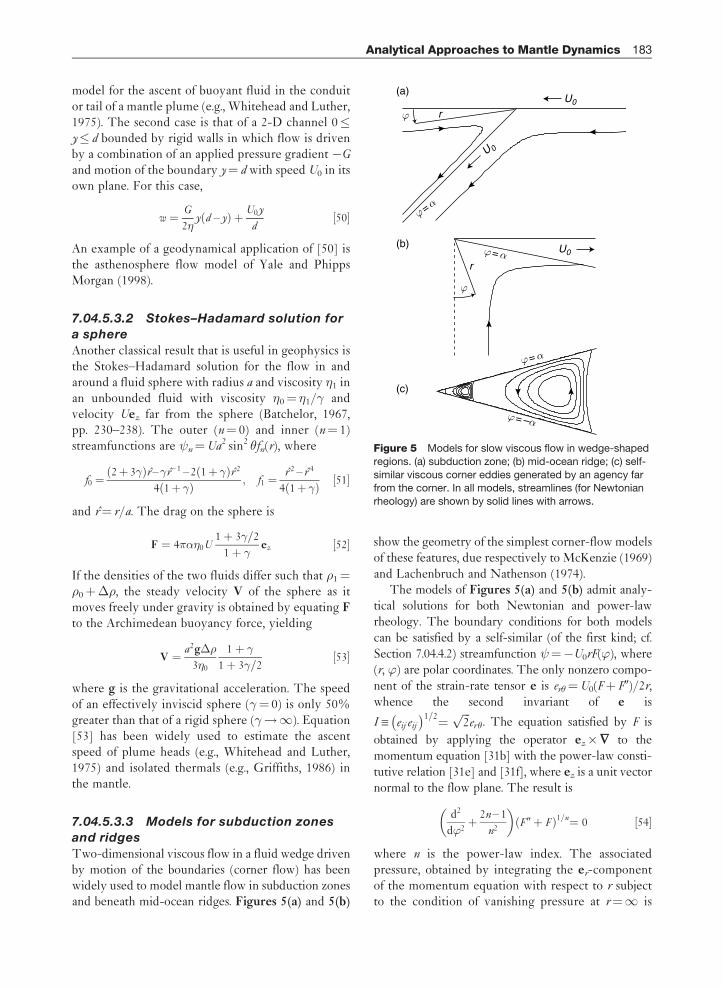
Two-dimensional viscous flow in a fluid wedge drivenby motion of the boundaries (corner flow) has beenwidely used to model mantle flow in subduction zonesand beneath mid-ocean ridges. Figures 5(a) and 5(b)

show the geometry of the simplest corner-flow modelsof these features, due respectively to McKenzie (1969)and Lachenbruch and Nathenson (1974).

The models of Figures 5(a) and 5(b) admit analy-tical solutions for both Newtonian and power-lawrheology. The boundary conditions for both modelscan be satisfied by a self-similar (of the first kind; cf.Section 7.04.4.2) streamfunction ¼�U0rF(’), where(r, ’) are polar coordinates. The only nonzero compo-nent of the strain-rate tensor e is er�¼U0(Fþ F0)/2r,whence the second invariant of e is

I X eij eij

� �1=2¼ffiffiffi2p

er�. The equation satisfied by F is

obtained by applying the operator ez�� to themomentum equation [31b] with the power-law consti-tutive relation [31e] and [31f], where ez is a unit vectornormal to the flow plane. The result is

d2

d’2þ 2n – 1

n2

� �F 0þ Fð Þ1=n¼ 0 ½54�

where n is the power-law index. The associatedpressure, obtained by integrating the er-componentof the momentum equation with respect to r subjectto the condition of vanishing pressure at r¼1 is

(a)

(b)

(c)

U0

U0

U 0

r

r

ϕ = α

ϕ = α

ϕ

ϕ

ϕ = α

ϕ = –α

Figure 5 Models for slow viscous flow in wedge-shaped

regions. (a) subduction zone; (b) mid-ocean ridge; (c) self-

similar viscous corner eddies generated by an agency farfrom the corner. In all models, streamlines (for Newtonian

rheology) are shown by solid lines with arrows.


p¼��U0r�1 (F9þ F-). Equation [54] can be solvedanalytically if n is any positive integer (Tovish et al.,1978). The values most relevant to geophysics (seeChapter 1.02) are n¼ 1 and n¼ 3, for which thegeneral solutions are

F1 ¼ A1sin’þ B1cos’þ C1’sin’þ D1’cos’ ½55�

F3 ¼ A3sin’þ B3cos’þ C3H ’; D3ð Þ ½56�

respectively, where

H ’; D3ð Þ ¼ 27 cos

ffiffiffi5p

3’þ D3ð Þ – cos

ffiffiffi5p

’þ D3ð Þ ½57�

and An�Dn are arbitrary constants for n¼ 1 andn¼ 3 that are determined by the boundary condi-tions. For the ridge model,

A1; B1; C1; D1f g ¼ c2; 0; 0; – 1f g – sc

½58�

A3; B3; C3; D3f g

¼ –C3 h1s þ h91cð Þ; 0;1

h91s – h1c;

3�

2ffiffiffi5p

�½59�

where s¼ sin, c¼ cos, h1¼H(, D3), andh91¼H’(, D3). For the Newtonian (n¼ 1) subduc-tion model in the wedge 0�’�,

A1; B1; C1; D1f g ¼ s; 0; c – s; –sf g2 – s2

½60�

For the power-law (n¼ 3) subduction model in0�’�, D3 satisfies h1� h0c� h90s¼ 0 and theother constants are

C3 ¼ h91 þ h0s – h90cð Þ – 1; B3 ¼ – h0C3;

A3 ¼ – h90C3 ½61�

where h0¼H (0, D3), and h90¼H’(0, D3). If needed,the solutions in the wedge �’� � can be obtainedfrom [55] and [56] by applying the boundary condi-tions shown in Figure 5(a). The solution [60]together with the corresponding one for the wedge�’� � was the basis for Stevenson and Turner’s(1977) hypothesis that the angle of subduction iscontrolled by the balance between the hydrodynamiclifting torque and the opposing gravitational torqueacting on the slab. Their results were extended topower-law fluids by Tovish et al. (1978).

7.04.5.3.4 Viscous eddies

Another important exact solution for slow viscousflow describes viscous eddies near a sharp corner(Moffatt, 1964). This solution is an example of aself-similar solution of the second kind (Section

7.04.4.2), the determination of which requires the

solution of an eigenvalue problem. Here we consider

only Newtonian fluids; for power-law fluids, see

Fenner (1975).The flow domain is a 2-D wedge j’j � bounded

by rigid walls (Figure 5(c)). Flow in the wedge is

driven by an agency (e.g., stirring) acting at a distance

�r0 from the corner. We seek to determine the

asymptotic character of the flow near the corner,

that is, in the limit r/r0! 0. Because the domain of

interest is far from the driving agency, we anticipate

that the flow will be self-similar.The streamfunction satisfies the biharmonic equa-

tion [37], which admits separable solutions of the

form

¼ r�F ’ð Þ ½62�

Substituting [62] into [37], we find that F satisfies

F 00þ �2 þ � – 2ð Þ2

F 0þ �2 � – 2ð Þ2¼ 0 ½63�

where primes denote d/d’. For all � except 0, 1, and2, the solution of [63] is

F ¼ A cos�’þ B sin�’þ C cos � – 2ð Þ’þ D sin � – 2ð Þ’ ½64�

where A–D are arbitrary constants. The solutions for�¼ 0, 1, and 2 do not exhibit eddies (the solutionwith �¼ 1 is the one used in the models of subduc-tion zones and ridges in Section 7.04.5.3.3).

The most interesting solutions are those for which (r, ’) is an even function of ’. Application of the

rigid-surface boundary conditions F()¼ F9()¼ 0

to [64] with B¼D¼ 0 yields two equations for A and C

that have a nontrivial solution only if

sin 2 � – 1ð Þþ � – 1ð Þsin 2 ¼ 0 ½65�

The only physically relevant roots of [65] are thosewith R(�) > 0, corresponding to solutions that arefinite at r¼ 0. When 2< 146 , these roots are allcomplex; let �1 X p1þ iq1 be the root with the smallestreal part, corresponding to the solution that decaysleast rapidly towards the corner. Figure 5(c) showsthe streamlines R(r�F)¼ cst for 2¼ 30 , for whichp1¼ 4.22 and q1¼ 2.20. The flow comprises an infi-nite sequence of self-similar eddies with alternatingsenses of rotation, whose successive intensitiesdecrease by a factor exp(�p1/q1) 414 towards thecorner. In the limit ¼ 0 corresponding to flowbetween parallel planes, p1¼ 4.21 and q1¼ 2.26,all the eddies have the same size (2.78 times thechannel width), and the intensity ratio 348.


In a geophysical context, corner eddies are signif-icant primarily as a simple model for the tendency offorced viscous flows in domains with large aspectratio to break up into separate cells. An example(Section 7.04.9.3), is steady 2-D cellular convectionat high Rayleigh number, in which Stokes flow in theisothermal core of a cell is driven by the shear stressesapplied to it by the thermal plumes at its ends. Whenthe aspect ratio (width/depth) �¼ 1, the core flowcomprises a single cell ; but when �¼ 2.5, the flowseparates into two distinct eddies (Jimenez andZufiria, 1987, Figure 2).

7.04.5.4 Superposition and EigenfunctionExpansion Methods

The linearity of the equations governing Stokes flowis the basis of two powerful methods for solvingStokes flow problems in regular domains: themethods of superposition and eigenfunction expan-sion. In both methods, a complicated flow isrepresented by infinite sums of elementary separablesolutions of the Stokes equations for the coordinatesystem in question, and the unknown coefficients inthe expansion are determined to satisfy the boundaryconditions. In the superposition method, theindividual separable solutions do not themselvessatisfy all the boundary conditions in any of thecoordinate directions. In the method of eigenfunctionexpansions (henceforth MEE), by contrast, the separ-able solutions are true eigenfunctions that satisfy allthe (homogeneous) boundary conditions at both endsof an interval in one of the coordinate directions, sothat the unknown constants are determined entirelyby the boundary conditions in the other direction(s).Let us turn now to some concrete illustrationsof these methods in three coordinate systems ofgeophysical interest: 2-D Cartesian, spherical, andbispherical.

7.04.5.4.1 2-D flow in Cartesian

coordinates

The streamfunction for 2-D Stokes flow satisfiesthe biharmonic equation [37], which has the generalsolution

¼ f1 x þ iyð Þ þ f2 x – iyð Þ þ y þ ixð Þf3 x þ iyð Þþ y – ixð Þf4 x – iyð Þ ½66�

where f1–f4 are arbitrary functions of their (complex)arguments. However, the most useful solutionsfor applications are the separable solutions that

vary periodically in one direction. Setting _ exp ikx and solving [37] by separation of vari-ables, we find

¼ ½ A1 þ A2yð Þexp – kyð Þþ A3 þ A4yð Þexp ky�exp ikx ½67�

where A1–A4 are arbitrary functions of k. Ananalogous solution is obtained by interchanging x

and y in [67], and both solutions remain valid if k iscomplex.

The solution [67] has been widely used in geody-namics to describe flows generated by loads that vary

sinusoidally in the horizontal direction (e.g., Fleitout

and Froidevaux, 1983.) The representation of more

general flows, however, typically requires the use of a

superposition or an eigenfunction expansion. To

illustrate the use of these two methods, we consider

the problem of driven cavity flow in a rectangular

domain x P [��/2, �/2], y P [�1/2, 1/2] with

impermeable ( ¼ 0) boundaries (Figure 6). The

sidewalls x¼�/2 and the bottom y¼�1/2 are

rigid and motionless, while the upper boundary

y¼ 1/2 moves in its own plane with velocity U(x)

(Figure 6, boundary conditions a).In the superposition method, the solution is repre-

sented as a sum of two ordinary Fourier series in

the two coordinate directions. The flow is the sum

of two parts that are even and odd functions of y,

(a) ψx = 0

(a) ψx = 0

(a) ψy = –U(x)

(b) ψy = 0 (rigid) or ψyy = 0 (free)

(b) ψy = 0 (rigid) or ψyy = 0 (free)

(a) ψy = 0

(b) ψx ψxx = – 1/2

(b) ψx ψxx = 1/2

–1/2

1/2

– β /2 β /2

x

y

Figure 6 Geometry and boundary conditions for (a) driven

cavity flow and (b) steady cellular convection in a rectanglex P[��/2, �/2], y P[�1/2, 1/2] with impermeable

boundaries. All lengths are nondimensionalized by the

height of the rectangle.


respectively, and the representation for the even partis (Meleshko, 1996)

¼X1m¼1

AmF y; pm; 1� �

cos pmx

þX1n¼1

BnF x; qn; �ð Þcos qny ½68a�

pm ¼2m – 1

��; qn ¼ 2n – 1ð Þ� ½68b�

F z; k; rð Þ ¼ r tanh rk=2ð Þcosh kz – 2z sinh kz

2 cosh rk=2ð Þ ½68c�

where Am and Bn are undetermined coefficients. Dueto the choice of the wave numbers pm and qn and thefunction F(z,k,r) (which vanishes at z¼r/2), each ofthe series in [68a] satisfies the impermeability condi-tion ¼ 0 on all boundaries. Moreover, because thetrigonometric systems cos pmx and cos qny are com-plete, the superposition [68] (with suitable choices ofAm and Bn) can represent arbitrary distributions oftangential velocity on y¼1/2 and x¼�/2.

Unlike the superposition method, the MEE makesuse of so-called Papkovich–Fadle eigenfunctions�(x) that satisfy all the homogeneous boundary con-ditions in the direction (x in this case) perpendicularto two motionless walls. For simplicity, suppose thatU(x)¼U (�x), so that is an even function of x. Theeven eigenfunctions on the canonical unit interval x

P [�1/2, 1/2] are obtained by substituting ¼�(x)exp(�y) into the biharmonic equation [37] and sol-ving the resulting equation for � subject to theconditions �(1/2)¼�x(1/2)¼ 0, yielding

�n xð Þ ¼ x sin�nx –1

2tan

�n

2cos�nx ½69�

where �n are the first-quadrant complex roots of sin�nþ�n¼ 0. The streamfunction for the flow in thecavity with x P [��/2,�/2] (Figure 6) can then bewritten as (Shankar, 1993)

¼X1n¼1

(An�n exp –�n y þ 1

2

� ��

þ �An��n exp – ��n y þ 1

2

� ��

þ Bn�n exp –�n

1

2– y

� ��

þ �Bn��n exp – ��n

1

2– y

� �� )½70�

where �n¼�n(x/�), overbars denote complex con-jugation, and the constants An and Bn are chosen to

satisfy the boundary conditions at y¼1/2. Thedifficulty, however, is that the reduced biharmonicequation (d2/dx2þ�2)2�¼ 0 satisfied by the eigen-functions �n is not self-adjoint, as can be seen byrewriting it in the form

d2

dx2

�

–� – 2�0

!¼ �2

0 – 1

1 – 2

!�

–� – 2�0

!½71�

and noting that the square matrix on the RHS is notHermitian. Consequently, the eigenfunctions �n arenot mutually orthogonal, which makes the determi-nation of An and Bn a nontrivial matter. One solutionis to use a complementary set of adjoint eigenfunc-tions �m which are biorthogonal to the set �n,although considerable care must then be taken toensure convergence of the expansion (seeKatopodes et al. (2000) for a discussion and referencesto the relevant literature). A cruder but very effectiveapproach is to determine An and Bn via a numericalleast-squares procedure that minimizes the misfit ofthe solution [70] to the boundary conditions(Shankar, 1993; Bloor and Wilson, 2006). Shankar(2005) showed how this approach can be extendedto an irregular domain by embedding the latter in alarger, regular domain on which a complete set ofeigenfunctions exists.

Another geophysically relevant 2-D Stokes pro-blem that can be solved using superposition andeigenfunction expansion methods is that of the flowwithin the isothermal core of a vigorous (highRayleigh number) convection cell. The boundaryconditions for this case (Figure 6, conditions b) com-prise either rigid ( y¼ 0) or traction-free ( yy¼ 0)conditions at y¼1/2 and nonlinear sidewall con-ditions x xx¼1/2 (derived in Section 7.04.9.3.2)that represent the shear stresses applied to the coreby the buoyant thermal plumes. If the boundariesy¼1/2 are traction free, the conditions ¼ yy¼ 0involve only even derivatives of , and are satisfiedidentically if _ cos qny where qn is defined by [68b].The streamfunction that also satisfies the sidewallimpermeability conditions (�/2, y)¼ 0 is(Roberts, 1979)

¼X1n¼0

AnF x; qn; �ð Þcos qny ½72�

where F(x, qn, �) is defined by [68c]. The constants An

are then determined iteratively to satisfy the bound-ary conditions x xx (�/2, y)¼1/2. Strictlyspeaking, [72] is an eigenfunction expansion, becausethe functions cosqny satisfy all the homogeneous


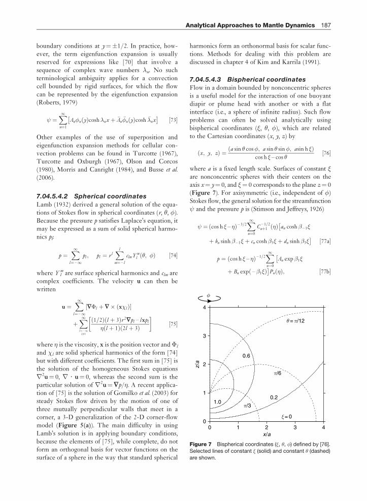
boundary conditions at y¼1/2. In practice, how-ever, the term eigenfunction expansion is usuallyreserved for expressions like [70] that involve asequence of complex wave numbers �n. No suchterminological ambiguity applies for a convectioncell bounded by rigid surfaces, for which the flowcan be represented by the eigenfunction expansion(Roberts, 1979)

¼X1n¼1

An�n yð Þcosh�nx þ �An��n yð Þcosh ��nx

½73�

Other examples of the use of superposition andeigenfunction expansion methods for cellular con-vection problems can be found in Turcotte (1967),Turcotte and Oxburgh (1967), Olson and Corcos(1980), Morris and Canright (1984), and Busse et al.

(2006).

7.04.5.4.2 Spherical coordinates

Lamb (1932) derived a general solution of the equa-tions of Stokes flow in spherical coordinates (r, �, �).Because the pressure p satisfies Laplace’s equation, itmay be expressed as a sum of solid spherical harmo-nics pl:

p ¼X1

l¼ –1pl ; pl ¼ r l

Xl

m¼ – l

clmY ml �; �ð Þ ½74�

where Y lm are surface spherical harmonics and clm are

complex coefficients. The velocity u can then bewritten

u ¼X1

l¼ –1��l þ �� x�lð Þ½ �

þX1l¼ –1

l 6¼1

1=2ð Þ l þ 3ð Þr 2�pl – lxpl

� l þ 1ð Þ 2l þ 3ð Þ

� �½75�

where � is the viscosity, x is the position vector and �l

and �l are solid spherical harmonics of the form [74]but with different coefficients. The first sum in [75] isthe solution of the homogeneous Stokes equationsr2u¼ 0, r ? u¼ 0, whereas the second sum is theparticular solution of r2u¼�p/�. A recent applica-tion of [75] is the solution of Gomilko et al. (2003) forsteady Stokes flow driven by the motion of one ofthree mutually perpendicular walls that meet in acorner, a 3-D generalization of the 2-D corner-flowmodel (Figure 5(a)). The main difficulty in usingLamb’s solution is in applying boundary conditions,because the elements of [75], while complete, do notform an orthogonal basis for vector functions on thesurface of a sphere in the way that standard spherical

harmonics form an orthonormal basis for scalar func-tions. Methods for dealing with this problem arediscussed in chapter 4 of Kim and Karrila (1991).

7.04.5.4.3 Bispherical coordinatesFlow in a domain bounded by nonconcentric spheresis a useful model for the interaction of one buoyantdiapir or plume head with another or with a flatinterface (i.e., a sphere of infinite radius). Such flowproblems can often be solved analytically usingbispherical coordinates (�, �, �), which are relatedto the Cartesian coordinates (x, y, z) by

x; y; zð Þ ¼ a sin � cos�; a sin � sin�; asin h �ð Þcos h � – cos �

½76�

where a is a fixed length scale. Surfaces of constant �are nonconcentric spheres with their centers on theaxis x¼ y¼ 0, and �¼ 0 corresponds to the plane z¼ 0(Figure 7). For axisymmetric (i.e., independent of �)Stokes flow, the general solution for the streamfunction and the pressure p is (Stimson and Jeffreys, 1926)

¼ cos h � – �ð Þ – 3=2X1n¼0

C– 1=2

nþ1 �ð Þan cosh� – 1�

þ bn sinh � – 1� þ cn cosh �3� þ dn sinh �3�½77a�

p ¼ cos h � – �ð Þ – 1=2X1n¼0

An exp�1�

þ Bn exp – �1�ð ÞPn �ð Þ; ½77b�

0

1

2

3

4

0 1 2 3 4

θ = π/12

x /a

z /a

π/6

φ

π/3

ξ = 0

1.0

0.6

0.2

Figure 7 Bispherical coordinates (�, �, �) defined by [76].

Selected lines of constant � (solid) and constant � (dashed)

are shown.


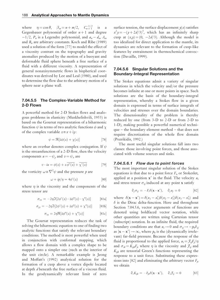
where �¼ cos �, �m¼ nþm/2, Cnþ 1�1/2 is a

Gegenbauer polynomial of order nþ 1 and degree�1/2, Pn is a Legendre polynomial, and an� dn, An,and Bn are arbitrary constants. Koch and Ribe (1989)used a solution of the form [77] to model the effect ofa viscosity contrast on the topography and gravityanomalies produced by the motion of a buoyant anddeformable fluid sphere beneath a free surface of afluid with a different viscosity. A representation ofgeneral nonaxisymmetric flows in bispherical coor-dinates was derived by Lee and Leal (1980), and usedto determine the flow due to the arbitrary motion of asphere near a plane wall.

7.04.5.5 The Complex-Variable Method for2-D Flows

A powerful method for 2-D Stokes flows and analo-gous problems in elasticity (Muskhelishvili, 1953) isbased on the Goursat representation of a biharmonicfunction in terms of two analytic functions � and �of the complex variable z X xþ iy :

¼ R �z� zð Þ þ � zð Þ½ � ½78�

where an overbar denotes complex conjugation. If is the streamfunction of a 2-D flow, then the velocitycomponents u¼� y and v¼ x are

v – iu ¼ � zð Þ þ z�9 zð Þ þ �9 zð Þ ½79�

the vorticity ! Xr2 and the pressure p are

!þ ip=� ¼ 4�9 zð Þ ½80�

where � is the viscosity and the components of thestress tensor are

�xx ¼ – 2�I 2�9 zð Þ – �z�0 zð Þ –�0 zð Þ½ � ½81a�

�yy ¼ – 2�I 2�9 zð Þ þ �z�0 zð Þ þ �0 zð Þ½ � ½81b�

�xy ¼ 2�R �z�0 zð Þ þ �0 zð Þ½ � ½81c�

The Goursat representation reduces the task ofsolving the biharmonic equation to one of finding twoanalytic functions that satisfy the relevant boundaryconditions. The method is most powerful when usedin conjunction with conformal mapping, whichallows a flow domain with a complex shape to bemapped onto a simpler one (such as the interior ofthe unit circle). A remarkable example is Jeongand Moffatt’s (1992) analytical solution for theformation of a cusp above a vortex dipole locatedat depth d beneath the free surface of a viscous fluid.In the geodynamically relevant limit of zero

surface tension, the surface displacement y(x) satisfiesx2y¼�(yþ 2d/3)3, which has an infinitely sharpcusp at (x,y)¼ (0, �2d/3). Although the model istoo idealized for direct application to the mantle, itsdynamics are relevant to the formation of cusp-likefeatures by entrainment in thermochemical convec-tion (Davaille, 1999).

7.04.5.6 Singular Solutions and theBoundary-Integral Representation

The Stokes equations admit a variety of singularsolutions in which the velocity and/or the pressurebecomes infinite at one or more points in space. Suchsolutions are the basis of the boundary-integralrepresentation, whereby a Stokes flow in a givendomain is expressed in terms of surface integrals ofvelocities and stresses over the domain boundaries.The dimensionality of the problem is therebyreduced by one (from 3-D to 2-D or from 2-D to1-D), making possible a powerful numerical techni-que – the boundary element method – that does notrequire discretization of the whole flow domain(Pozrikidis, 1992.)

The most useful singular solutions fall into twoclasses: those involving point forces, and those asso-ciated with volume sources and sinks.

7.04.5.6.1 Flow due to point forces

The most important singular solution of the Stokesequations is that due to a point force Fi, or Stokeslet,applied at a position x9 in the fluid. The velocity ui

and stress tensor �ij induced at any point x satisfy

qj�ij ¼ – Fi� x – x9ð Þ; qj uj ¼ 0 ½82�

where �(x� x9)¼ �(x1� x91)�(x2� x92)�(x3� x93) and� is the Dirac delta-function. Here and throughoutSection 7.04.5.6, vector arguments of functions aredenoted using boldfaced vector notation, whileother quantities are written using Cartesian tensor(subscript) notation. In an infinite fluid, the requiredboundary conditions are that ui! 0 and �ij!�p0�ij

as jx� x9j!1, where p0 is the (dynamically irrele-vant) far-field pressure. Because the response of thefluid is proportional to the applied force, ui¼ JijFj/�and �ik¼ KijkFj, where � is the viscosity and Jij andKijk are tensorial Green’s functions representing theresponse to a unit force. Substituting these expres-sions into [82] and eliminating the arbitrary vector Fj,we obtain

qiKijk ¼ – �jk� x – x9ð Þ; qi Jij ¼ 0 ½83�


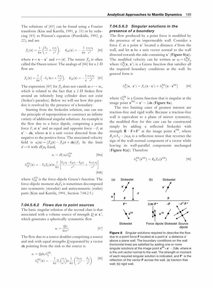
The solutions of [83] can be found using a Fouriertransform (Kim and Karrila, 1991, p. 33) or by redu-cing [83] to Poisson’s equation (Pozrikidis, 1992, p.22), and are

Jij rð Þ ¼ 1

8�

�ij

rþ ri rj

r 3

� �; Kijk rð Þ ¼ –

3

4�

ri rj rk

r 5½84�

where r¼ x� x9 and r¼ jrj. The tensor Jij is oftencalled the Oseen tensor. The analogs of [84] for a 2-Dflow are

Jij rð Þ ¼ 1

4�– �ij ln r þ ri rj

r 2

� �; Kijk rð Þ ¼ –

1

�

ri rj rk

r 4½85�

The expression [85] for Jij does not vanish as r!1,which is related to the fact that a 2-D Stokes flowaround an infinitely long cylinder does not exist(Stokes’s paradox). Below we will see how this para-dox is resolved by the presence of a boundary.

Starting from the Stokeslet solution, one can usethe principle of superposition to construct an infinitevariety of additional singular solutions. An example isthe flow due to a force dipole, comprising a pointforce Fi at x9 and an equal and opposite force �Fi atx9� dn, where n is a unit vector directed from thenegative to the positive force. The associated velocityfield is ui(x)¼ [Jij(r)� Jij(rþ dn)]Fj. In the limitd! 0 with dFjnk fixed,

ui ¼ dFj nkGFDijk ½86a�

GFDijk rð Þ ¼ – qkJij rð ÞX 1

8�

�ij rk – �ikrj – �jkri

r 3þ 3ri rj rk

r 5

� �

½86b�

where GijkFD is the force-dipole Green’s function. The

force-dipole moment dnjFk is sometimes decomposedinto symmetric (stresslet) and antisymmetric (rotlet)parts (Kim and Karrila, 1991, Section 7.04.2.5.)

7.04.5.6.2 Flows due to point sources

The basic singular solution of the second class is thatassociated with a volume source of strength Q at x9,which generates a spherically symmetric flow

ui ¼Qri

4�r 3½87�

The flow due to a source doublet comprising a sourceand sink with equal strengths Q separated by a vectordn pointing from the sink to the source is

ui ¼ Qdnj GSDij ;

GSDij rð Þ ¼ –

1

4�qj

ri

r 3

� �X

1

4�

3ri rj

r 5–�ij

r 3

� � ½88�

7.04.5.6.3 Singular solutions in the

presence of a boundary

The flow produced by a point force is modified by

the presence of an impermeable wall. Consider a

force Fi at a point x9 located a distance d from the

wall, and let n be a unit vector normal to the wall

directed towards the side containing x9 (Figure 8(a)).

The modified velocity can be written as ui¼GijBFj,

where GijB(x, x9) is a Green function that satisfies all

the required boundary conditions at the wall. Its

general form is

GBij x; x9ð Þ ¼ Jij x – x9ð Þ þ GIM

ij x – xIM� �

½89�

where GijIM is a Green function that is singular at the

image point xIM¼ x9� 2dn (Figure 8a).The two limiting cases of greatest interest are

traction-free and rigid walls. Because a traction-free

wall is equivalent to a plane of mirror symmetry,

the modified flow for this case can be constructed

simply by adding a reflected Stokeslet with

strength R ? F XF� at the image point xIM, where

Rij X �ij� 2ninj is a reflection tensor that reverses the

sign of the wall-normal component of a vector while

leaving its wall-parallel components unchanged

(Figure 8(a)). Therefore

GIMij rIM� �

¼ RjkJik rIM� �

½90�

(a) (b)

Source dipole

ForceStokeslet

Stokeslet Stokeslet

x ′

–d 2 F *

dn

F *

F F

–F2d n F *

x

IMxIM

x′

dipole Stokeslet

Figure 8 Singular solutions required to describe the flow

due to a point force F located at a point x9 a distance d

above a plane wall. The boundary conditions on the wall(horizontal lines) are satisfied by adding one or more

singular solutions at the image point xIMX x9�2dn, where n

is the unit vector normal to the wall. The strength or moment

of each required singular solution is indicated, and F� is thereflection of the vector F across the wall. (a) traction-free

wall; (b) rigid wall.


where rIM¼ x� xIM. If the surface is rigid, theboundary conditions can be satisfied by addingthree different singular solutions at xIM: a Stokesletwith strength �F, a force dipole with moment2dnF�, and a source dipole with strength �d2F�

(Figure 8(b)) The result is (Blake, 1971)

GIMij rIM� �

¼ – Jij rIM� �

þ 2dRjl nkGFDikl rIM� �

– d 2RjkGSDik rIM� �

½91�

where GijFD and Gij

SD are defined by [86b] and [88],respectively.

Expressions analogous to those above also applyto 2-D flow in the presence of a boundary. Thebasic idea is illustrated by the free-surface case, for

which both [89] and [90] remain valid if Jij has its

2-D form [85]. Now, however, the presence of the

image singularity GijIM cancels the logarithmic

divergence of Jij at large distances from the point

force, thereby resolving Stokes’s paradox and ren-

dering the problem well-posed. A rigid surface hasthe same effect, although the corresponding expres-

sions for the Green’s function are more

complicated.

7.04.5.6.4 Boundary-integral

representation

The boundary-integral representation for Stokes

flow expresses the velocity ui at any point in a fluidvolume V bounded by a surface S in terms of the

velocity and traction on S. The starting point is

the integral form [34] of the Lorentz reciprocal the-

orem. Let (ui, �ij) be the flow of interest in a fluidwith no distributed body forces (bi¼ 0), and let

ui�X Jij(x� x9)Fj/� and �ik

�XKijk(x� x9)Fj be the

flow produced by a point force bi�X Fi�(x� x9) at

the point x9. Substituting these expressions into [34]

and dropping the arbitrary vector Fi, we obtain

1

�

ZS

Jij x – x9ð Þ�ik xð Þnk xð ÞdS xð Þ –Z

V

uj xð Þ� x – x9ð ÞdV xð Þ

¼Z

S

Kijk x – x9ð Þui xð Þnk xð ÞdS xð Þ ½92�

where the normal n points out of V. Now

ZV

uj xð Þ� x – x9ð ÞdV ¼ � x9ð Þuj x9ð Þ ½93�

where �(x9)¼ 0, 1/2, or 1 depending on whether x9

lies outside V, right on S, or inside V, respectively.Substituting [93] into [92] and interchanging the

roles of x and x9, we obtain the boundary-integralrepresentation

1

�

ZS9

Jij�iknkdS9 –

ZS9

KijkuinkdS9 ¼ � xð Þuj xð Þ ½94�

where the arguments of the quantities in the integrands(x9 for nk, �ik, and ui ; x9� x for Jij and Kijk) have beensuppressed for brevity and dS9¼ dS(x9). The first inte-gral in [94] represents the velocity due to a surfacedistribution of point forces with density �iknk dS9. It iscalled the single-layer potential by analogy to theelectrostatic potential generated by a surface distribu-tion of electric charges. The second integral, called thedouble-layer potential, represents the velocity fieldgenerated by the sum of a distribution of sources andsinks and a symmetric distribution of force dipoles(Kim and Karrila, 1991, Section 7.04.2.4.2).

An important extension of the integral representa-tion [94] is to the buoyancy-driven motion of a fluiddrop with viscosity �2 X ��1 and density �2 X �1þ��in another fluid with viscosity �1 and density �1

(Pozrikidis, 1990; Manga and Stone, 1993.) Let S,V1, and V2 be the surface of the drop and the volumesoutside and inside it, respectively. We begin by writ-ing separate integral equations of the form [94] foreach fluid:

–1

�1

ZS9

Jij�1ð Þ

ik nkdS9þZ

S9

Kijku1ð Þ

i nkdS9

¼ �1 xð Þu 1ð Þj xð Þ ½95a�

1

�2

ZS9

Jij�2ð Þ

ik nkdS9 –

ZS9

Kijku2ð Þ

i nkdS9

¼ �2 xð Þu 2ð Þj xð Þ ½95b�

where n points out of the drop and the volume (V1 orV2) in which a given quantity is defined as indicatedby a superscript in parentheses. Here �1(x)¼ 0, 1/2,or 1 if x is in V2, right on S, or in V1, respectively, and�2(x) is defined similarly but with the subscripts 1and 2 interchanged. Now multiply [95b] by �, addthe result to [95a], and apply the matching conditionsuj

(1)¼ uj(2)¼ uj and (�ik

(1)� �ik(2))nk¼ ni��gkx9k on S,

where gk is the gravitational acceleration. The result is

�1 xð Þu 1ð Þj xð Þ þ ��2 xð Þu 2ð Þ

j xð Þ – 1 – �ð ÞZ

S9

Kijkui nkdS9

¼ –gk��

�1

ZS9

Jij ni x9kdS9 ½96�

For points x on S, [96] reduces to

1

2uj xð Þ – 1 – �

1þ �

ZS9

Kijkui nkdS9

¼ –gk��

�1 1þ �ð Þ

ZS9

Jij ni x9kdS9 x P Sð Þ ½97�


a Fredholm integral equation of the second kind forthe velocity u of the interface. Once u on S has beendetermined by solving [97], u at points in V1 and V2

can be determined if desired from [96]. A general-ization of [97] to N > 1 interacting drops was derivedby Manga and Stone (1993).

The integral equation [97], which must in generalbe solved numerically, has been used in geodynamicsto model systems comprising distinct fluids with dif-ferent viscosities. Manga and Stone (1993) solved theN-drop generalization of [97] using the boundaryelement method (Pozrikidis, 1992) to investigate thebuoyancy-driven interaction between two drops inan infinite fluid with a different viscosity. Manga et al.

(1993) used a similar method to study the interactionof plume heads with compositional discontinuities inthe Earth’s mantle. The deformation of viscous blobsin a 2-D cellular flow was investigated by Manga(1996), who concluded that geochemical reservoirscan persist undisturbed for relatively long times ifthey are 10–100 times more viscous than the sur-rounding mantle. Finally, Manga (1997) showedthat the deformation-induced mutual interactions ofdeformable diapirs in a rising cloud causes the diapirsprogressively to cluster, but that the rate of thisclustering is probably too slow to affect significantlythe lateral spacing of rising diapirs in the mantle.

7.04.5.7 Slender-Body Theory

Slender-body theory (SBT) is concerned with Stokesflow around thin rod-like bodies whose length greatlyexceeds their other two dimensions. The approachtakes its departure from Stokes’s paradox: the factthat a solution of the equations for Stokes flow aroundan infinitely long circular cylinder moving steadily inan unbounded viscous fluid does not exist, due to alogarithmic singularity that makes it impossible tosatisfy all the boundary conditions (Batchelor, 1967).However, the problem can be regularized in one ofthree ways: by including inertia, by making the lengthof the cylinder finite, or by making the domainbounded. SBT is concerned with the second (and byextension the third) of these possibilities.

The canonical problem of SBT is to determine theforce F on a rod of length 2, and radius a� , movingwith uniform velocity U in a viscous fluid. The solu-tion can be found using the MMAE, which exploitsthe fact that the flow field comprises two distinctregions characterized by very different length scales.The first or inner region includes points whose radialdistance � from the rod is small compared to their

distance from the rod’s nearer end. In this region, thefluid is not affected by the ends of the rod, and sees itas an infinite cylinder with radius a. The second, outerregion �� a is at distances from the rod that are largecompared to its radius. Here, the fluid is unaffected bythe rod’s finite radius, and sees it as a line distributionof point forces with effectively zero thickness. Thebasic idea of the MMAE is to obtain two differentasymptotic expansions for the velocity field that arevalid in the inner and outer regions, respectively, andthen to match them together in an intermediate oroverlap region where both expansions must coincide.

As the details of the matching are rather compli-cated, we defer our discussion of the method toSection 7.04.2, where it will be applied in the contextof BL theory. Here we simply quote the lowest-orderresult that the force on a cylinder whose axis isparallel to a unit vector ez is

F ¼ – 4��, 2U – U ? ezð Þez½ � ½98�

where ¼ (ln2,/a)�1. The force on a cylinder movingnormal to its axis (U ? ez¼ 0) is thus twice that on onemoving parallel to its axis. For further details andextensions of SBT, see Batchelor (1970), Cox (1970),Keller and Rubinow (1976), and Johnson (1980).Geophysically relevant applications of SBT includeOlson and Singer (1985), who used [98] to predict therise velocity of buoyant quasi-cylindrical (diapiric)plumes. Koch and Koch (1995) used an expressionanalogous to [98] for an expanding ring to model thebuoyant spreading of a viscous drop beneath the freesurface of a much more viscous fluid. Whittaker andLister (2006a) presented a model for a creeping plumeabove a planar boundary from a point source of buoy-ancy, in which they modeled the flow outside theplume as that due to a line distribution of Stokeslets.

7.04.5.8 Flow Driven by Internal Loads

Because inertia is negligible in the mantle, the flow ateach instant is determined entirely by the distribu-tion of internal density anomalies (loads) at thatinstant. This principle is the basis of a class of internalloading models in which an instantaneous mantleflow field is determined by convolving a load distri-bution with a Green function that represents themantle’s response to a unit load. However, it provesconvenient here to define the unit load not as a pointforce, but rather as a surface force concentrated at asingle radius and whose amplitude is proportional toa spherical harmonic Yl

m(�, �) of degree l and order m.


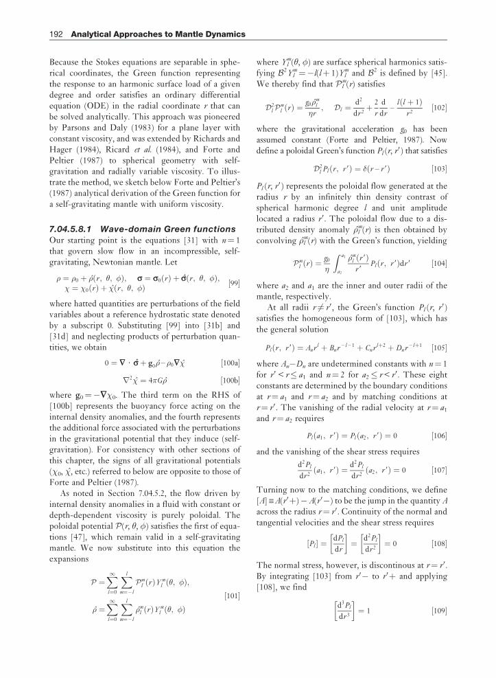
Because the Stokes equations are separable in sphe-rical coordinates, the Green function representingthe response to an harmonic surface load of a givendegree and order satisfies an ordinary differentialequation (ODE) in the radial coordinate r that canbe solved analytically. This approach was pioneeredby Parsons and Daly (1983) for a plane layer withconstant viscosity, and was extended by Richards andHager (1984), Ricard et al. (1984), and Forte andPeltier (1987) to spherical geometry with self-gravitation and radially variable viscosity. To illus-trate the method, we sketch below Forte and Peltier’s(1987) analytical derivation of the Green function fora self-gravitating mantle with uniform viscosity.

7.04.5.8.1 Wave-domain Green functionsOur starting point is the equations [31] with n¼ 1that govern slow flow in an incompressible, self-gravitating, Newtonian mantle. Let

� ¼ �0 þ � r ; �; �ð Þ; s ¼ s0 rð Þ þ s r ; �; �ð Þ;� ¼ �0 rð Þ þ � r ; �; �ð Þ ½99�

where hatted quantities are perturbations of the fieldvariables about a reference hydrostatic state denotedby a subscript 0. Substituting [99] into [31b] and[31d] and neglecting products of perturbation quan-tities, we obtain

0 ¼ � ? sþ g0� – �0�� ½100a�

r2� ¼ 4�G� ½100b�

where g0¼��0. The third term on the RHS of[100b] represents the buoyancy force acting on theinternal density anomalies, and the fourth representsthe additional force associated with the perturbationsin the gravitational potential that they induce (self-gravitation). For consistency with other sections ofthis chapter, the signs of all gravitational potentials(�0, �, etc.) referred to below are opposite to those ofForte and Peltier (1987).

As noted in Section 7.04.5.2, the flow driven byinternal density anomalies in a fluid with constant ordepth-dependent viscosity is purely poloidal. Thepoloidal potential P (r, �, �) satisfies the first of equa-tions [47], which remain valid in a self-gravitatingmantle. We now substitute into this equation theexpansions

P ¼X1l¼0

Xl

m¼ – l

P ml rð ÞY m

l �; �ð Þ;

� ¼X1l¼0

Xl

m¼ – l

�ml rð ÞY m

l �; �ð Þ½101�

where Ylm(�, �) are surface spherical harmonics satis-

fying B 2Ylm¼�l(lþ 1)Yl

m and B 2 is defined by [45].We thereby find that P l

m(r) satisfies

D 2l P m

l rð Þ ¼ g0�ml

�r; D l ¼

d2

dr 2þ 2

r

d

dr–

l l þ 1ð Þr 2

½102�

where the gravitational acceleration g0 has beenassumed constant (Forte and Peltier, 1987). Nowdefine a poloidal Green’s function Pl (r, r9) that satisfies

D 2l Pl r ; r 9ð Þ ¼ � r – r 9ð Þ ½103�

Pl (r, r9) represents the poloidal flow generated at theradius r by an infinitely thin density contrast ofspherical harmonic degree l and unit amplitudelocated a radius r9. The poloidal flow due to a dis-tributed density anomaly �l

m(r) is then obtained byconvolving �l

m(r) with the Green’s function, yielding

P ml rð Þ ¼ g0

�

Z a1

a2

�ml r 9ð Þr 9

Pl r ; r 9ð Þdr 9 ½104�

where a2 and a1 are the inner and outer radii of themantle, respectively.

At all radii r 6¼ r9, the Green’s function Pl (r, r9)satisfies the homogeneous form of [103], which has

the general solution

Pl r ; r 9ð Þ ¼ Anr l þ Bnr – l – 1 þ Cnr lþ2 þ Dnr – lþ1 ½105�

where An�Dn are undetermined constants with n¼ 1for r9 < r� a1 and n¼ 2 for a2� r < r9. These eightconstants are determined by the boundary conditionsat r¼ a1 and r¼ a2 and by matching conditions atr¼ r9. The vanishing of the radial velocity at r¼ a1

and r¼ a2 requires

Pl a1; r 9ð Þ ¼ Pl a2; r 9ð Þ ¼ 0 ½106�

and the vanishing of the shear stress requires

d2Pl

dr 2a1; r 9ð Þ ¼ d2Pl

dr 2a2; r 9ð Þ ¼ 0 ½107�

Turning now to the matching conditions, we define[A] X A(r9þ)� A(r9�) to be the jump in the quantity A

across the radius r¼ r9. Continuity of the normal andtangential velocities and the shear stress requires

Pl½ � ¼dPl

dr

� �¼ d2Pl

dr 2

� �¼ 0 ½108�

The normal stress, however, is discontinous at r¼ r9.By integrating [103] from r9� to r9þ and applying[108], we find

d3Pl

dr 3

� �¼ 1 ½109�


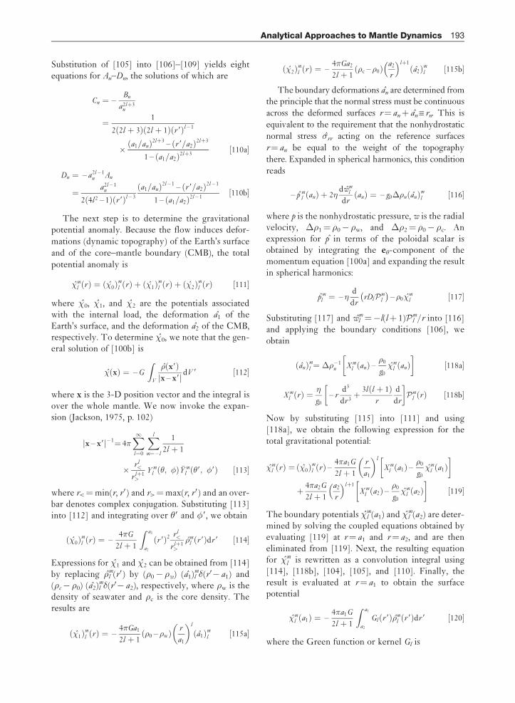
Substitution of [105] into [106]–[109] yields eightequations for An–Dn, the solutions of which are

Cn ¼ –Bn

a2lþ3n

¼ 1

2 2l þ 3ð Þ 2l þ 1ð Þ r 9ð Þl – 1

� a1=anð Þ2lþ3 – r 9=a2ð Þ2lþ3

1 – a1=a2ð Þ2lþ3½110a�

Dn ¼ – a2l – 1n An

¼ a2l – 1n

2 4l2 – 1ð Þ r 9ð Þl – 3

a1=anð Þ2l – 1 – r 9=a2ð Þ2l – 1

1 – a1=a2ð Þ2l – 1½110b�

The next step is to determine the gravitationalpotential anomaly. Because the flow induces defor-

mations (dynamic topography) of the Earth’s surface

and of the core–mantle boundary (CMB), the total

potential anomaly is

�ml rð Þ ¼ �0ð Þml rð Þ þ �1ð Þml rð Þ þ �2ð Þml rð Þ ½111�

where �0, �1, and �2 are the potentials associatedwith the internal load, the deformation a1 of theEarth’s surface, and the deformation a2 of the CMB,respectively. To determine �0, we note that the gen-eral solution of [100b] is

� xð Þ ¼ –G

ZV

� x9ð Þx – x9j j dV 9 ½112�

where x is the 3-D position vector and the integral isover the whole mantle. We now invoke the expan-sion (Jackson, 1975, p. 102)

x – x9j j – 1¼ 4�X1l¼0

Xl

m¼ – l

1

2l þ 1

� r l<

r lþ1>

Y ml �; �ð Þ �Y m

l �9; �9ð Þ ½113�

where r<¼min(r, r9) and r>¼max(r, r9) and an over-bar denotes complex conjugation. Substituting [113]into [112] and integrating over �9 and �9, we obtain

�0ð Þml rð Þ ¼ –4�G

2l þ 1

Z a1

a2

r 9ð Þ2 r l<

r lþ1>

�ml r 9ð Þdr 9 ½114�

Expressions for �1 and �2 can be obtained from [114]by replacing �l

m(r9) by (�0� �w) (a1)lm�(r9� a1) and

(�c� �0) (a2)lm�(r9� a2), respectively, where �w is the

density of seawater and �c is the core density. Theresults are

�1ð Þml rð Þ ¼ –4�Ga1

2l þ 1�0 – �wð Þ r

a1

� �l

a1ð Þml ½115a�

�2ð Þml rð Þ ¼ –4�Ga2

2l þ 1�c – �0ð Þ a2

r

� �lþ1

a2ð Þml ½115b�

The boundary deformations an are determined fromthe principle that the normal stress must be continuous

across the deformed surfaces r¼ anþ anX rn. This is

equivalent to the requirement that the nonhydrostatic

normal stress �rr acting on the reference surfaces

r¼ an be equal to the weight of the topography

there. Expanded in spherical harmonics, this condition

reads

– p ml anð Þ þ 2�

dwml

dranð Þ ¼ – g0��n anð Þml ½116�

where p is the nonhydrostatic pressure, w is the radialvelocity, ��1¼ �0� �w, and ��2¼ �0� �c. Anexpression for p in terms of the poloidal scalar isobtained by integrating the e�-component of themomentum equation [100a] and expanding the resultin spherical harmonics:

plm ¼ – �

d

drrDl P m

l

� �– �0�

ml ½117�

Substituting [117] and wlm¼�l(lþ 1)P l

m/r into [116]and applying the boundary conditions [106], weobtain

anð Þml ¼ �� – 1n X m

l anð Þ –�0

g0�m

l anð Þ� �

½118a�

X ml rð Þ ¼ �

g0– r

d3

dr 3þ 3l l þ 1ð Þ

r

d

dr

� �P m

l rð Þ ½118b�

Now by substituting [115] into [111] and using[118a], we obtain the following expression for thetotal gravitational potential:

�ml rð Þ ¼ �0ð Þml rð Þ – 4�a1G

2l þ 1

r

a1

� �l

X ml a1ð Þ –

�0

g0�m

l a1ð Þ� �

þ 4�a2G

2l þ 1

a2

r

� �lþ1

X ml a2ð Þ –

�0

g0�m

l a2ð Þ� �

½119�

The boundary potentials �lm(a1) and �l

m(a2) are deter-mined by solving the coupled equations obtained byevaluating [119] at r¼ a1 and r¼ a2, and are theneliminated from [119]. Next, the resulting equationfor �m

l is rewritten as a convolution integral using[114], [118b], [104], [105], and [110]. Finally, theresult is evaluated at r¼ a1 to obtain the surfacepotential

�ml a1ð Þ ¼ –

4�a1G

2l þ 1

Z a1

a2

Gl r 9ð Þ�ml r 9ð Þdr 9 ½120�

where the Green function or kernel Gl is


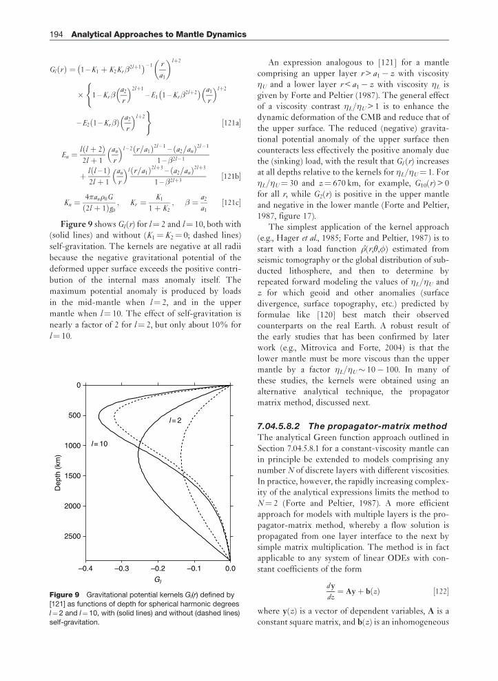
Gl rð Þ ¼ 1 –K1 þ K2Kr�2lþ1

� � – 1 r

a1

� �lþ2

�(

1 – Kr�a2

r

� �2lþ1

– E1 1 – Kr�2lþ2

� � a1

r

� �lþ2

– E2 1 –Kr�ð Þ a2

r

� �lþ2)

½121a�

En ¼l l þ 2ð Þ2l þ 1

an

r

� �l – 2 r=a1ð Þ2l – 1 – a2=anð Þ2l – 1

1 –�2l – 1

þ l l – 1ð Þ2l þ 1

an

r

� �l r=a1ð Þ2lþ3 – a2=anð Þ2lþ3

1 –�2lþ3½121b�

Kn ¼4�an�0G

2l þ 1ð Þg0; Kr ¼

K1

1þ K2; � ¼ a2

a1½121c�

Figure 9 shows Gl (r) for l¼ 2 and l¼ 10, both with(solid lines) and without (K1¼ K2¼ 0; dashed lines)

self-gravitation. The kernels are negative at all radii

because the negative gravitational potential of the

deformed upper surface exceeds the positive contri-

bution of the internal mass anomaly itself. The

maximum potential anomaly is produced by loads

in the mid-mantle when l¼ 2, and in the upper

mantle when l¼ 10. The effect of self-gravitation is

nearly a factor of 2 for l¼ 2, but only about 10% for

l¼ 10.

An expression analogous to [121] for a mantlecomprising an upper layer r > a1� z with viscosity�U and a lower layer r < a1� z with viscosity �L isgiven by Forte and Peltier (1987). The general effectof a viscosity contrast �L/�U > 1 is to enhance thedynamic deformation of the CMB and reduce that ofthe upper surface. The reduced (negative) gravita-tional potential anomaly of the upper surface thencounteracts less effectively the positive anomaly duethe (sinking) load, with the result that Gl (r) increasesat all depths relative to the kernels for �L/�U¼ 1. For�L/�U¼ 30 and z¼ 670 km, for example, G10(r) > 0for all r, while G2(r) is positive in the upper mantleand negative in the lower mantle (Forte and Peltier,1987, figure 17).

The simplest application of the kernel approach(e.g., Hager et al., 1985; Forte and Peltier, 1987) is tostart with a load function �(r,�,�) estimated fromseismic tomography or the global distribution of sub-ducted lithosphere, and then to determine byrepeated forward modeling the values of �L/�U andz for which geoid and other anomalies (surfacedivergence, surface topography, etc.) predicted byformulae like [120] best match their observedcounterparts on the real Earth. A robust result ofthe early studies that has been confirmed by laterwork (e.g., Mitrovica and Forte, 2004) is that thelower mantle must be more viscous than the uppermantle by a factor �L/�U� 10� 100. In many ofthese studies, the kernels were obtained using analternative analytical technique, the propagatormatrix method, discussed next.

7.04.5.8.2 The propagator-matrix method

The analytical Green function approach outlined inSection 7.04.5.8.1 for a constant-viscosity mantle canin principle be extended to models comprising anynumber N of discrete layers with different viscosities.In practice, however, the rapidly increasing complex-ity of the analytical expressions limits the method toN¼ 2 (Forte and Peltier, 1987). A more efficientapproach for models with multiple layers is the pro-pagator-matrix method, whereby a flow solution ispropagated from one layer interface to the next bysimple matrix multiplication. The method is in factapplicable to any system of linear ODEs with con-stant coefficients of the form

dy

dz¼ Ayþ b zð Þ ½122�

where y(z) is a vector of dependent variables, A is aconstant square matrix, and b(z) is an inhomogeneous

0

500

1000

1500

2000

2500

–0.4 –0.3 –0.2 –0.1 0.0

Dep

th (

km)

l = 2

l = 10

Gl

Figure 9 Gravitational potential kernels Gl(r) defined by

[121] as functions of depth for spherical harmonic degreesl¼2 and l¼10, with (solid lines) and without (dashed lines)

self-gravitation.


vector. The general solution of [122] is (Gantmacher,1960, I, p. 120, eqn [53])

y zð Þ ¼ P z; z0ð Þy z0ð Þ þZ z

z0

P z; ð Þb ð Þd ½123a�

P z; z0ð Þ ¼ exp A z – z0ð Þ½ � ½123b�

where y(z0) is the solution vector at the referencepoint z¼ z0 and P(z, z0) is the propagator matrix.The form of the solution [123] is identical to that fora scalar variable y(z), except that the argument of theexponential in [123b] is now a matrix rather than ascalar quantity. Analytical expressions for functionsof matrices such as [123b] are given by Gantmacher(1960, vol. I, pp. 95–110).

As an illustration, we determine the propagatormatrix for a poloidal flow driven by internal densityanomalies in a self-gravitating spherical shell withradially variable viscosity �(r) and laterally averageddensity �(r) (Hager and O’Connell, 1981; Richardsand Hager, 1984). As in Section 7.04.5.8.1, we supposethat the driving density anomaly is �l

m(r)Ylm(�,�),

where Ylm is a surface spherical harmonic.

The first step is to transform the equationsgoverning the flow in the mantle to the canonicalform [122], where A – to repeat – is a constantmatrix. The standard Stokes equations [31] for ourmodel mantle do not have this form for three rea-sons: (1) the fluid properties �(r) and �(r) vary withradius; (2) the expression for the differentialoperator � in spherical coordinates involves thescale factor r�1; and (3) a system of first-orderequations cannot be written in terms of theprimitive variables ui and p. Difficulty (1) is circum-vented by dividing the mantle into N discretelayers n¼ 1, 2,. . ., N, in each of which the viscosity�n and the density �n is constant. Difficulty (2) isovercome by using a transformed radial variablez¼ ln(r/a1), where a1 is the outer radius of themantle. Finally, one circumvents (3) by using theindependent variables

y ¼ u; v;r �rr

�0;

r �r�

�0;�0r �

�0;�0r 2qr �

�0

� �T

½124�

where u and v are the er- and e0-components of thevelocity, respectively, �0 and �0 are reference valuesof the viscosity and density, respectively, and thespherical harmonic dependence of each variable (u,�r r, �, and qr� _ Yl

m, v and �r� _ q�Ylm) has been

suppressed for clarity. The Stokes equations withineach layer n then takes the form [122] with

A ¼

– 2 L 0 0 0 0

– 1 1 0 1=�� 0 0

12�� – 6L�� 1 L 0 ��

– 6�� 2 2L – 1ð Þ�� – 1 – 2 �� 0

0 0 0 0 1 1

0 0 0 0 L 0

266666666664

377777777775

½125a�

b ¼0; 0; r 2g0 rð Þ� rð Þ=�0; 0; 0;

– 4�r 3G�0� rð Þ=�0

T ½125b�

where L¼ l (lþ 1), ��¼ �n/�0, and ��¼ �n/�0. Furthersimplification is achieved by recasting the densityanomaly �(r) as a sum of equivalent surface densitycontrasts �n (units kg m�2) localized at the midpoints rn

of the layers, according to

� rð Þ ¼X

n

� r – rnð Þ�n ½126�

In practice, �n is different in each layer, while �n and�n may be constant over several adjacent layers. For agroup of M such adjacent layers bounded by thedepths z and z0, the solution [123a] now takes theapproximate form

y zð Þ ¼ P z; z0ð Þy z0ð Þ þXMm¼1

P z; zmð Þbm ½127a�

bm ¼0; 0; rmg0 rmð Þ�m=�0; 0; 0;

– 4�r 2mG�0�m=�0

T ½127b�

where zm¼ ln(rm/a1). To use [127], one must applyboundary conditions at the CMB and at the Earth’ssurface, taking into account the dynamic topographyof these boundaries (Richards and Hager, 1984,Appendix 1).

An analytical expression for P(z, z0) can bewritten in terms of the minimal polynomial (�) ofA. For the matrix [125a], (�) is identical to thecharacteristic polynomial, and is

�ð Þ ¼Y4

i¼1

� –�ið Þmi ½128a�

�1 ¼ l þ 1; �2 ¼ – l ;

�3 ¼ l – 1; �4 ¼ – l – 2½128b�

m1 ¼ m2 ¼ 2; m3 ¼ m4 ¼ 1 ½128c�

where �1–�4 are the four distinct eigenvalues of A.Following Gantmacher (1960, I, pp. 95–102)

P z; z0ð Þ ¼X4

k¼1

Xmk

j¼1

kj A –�kIð Þj – 1�k ½129�


where

kj ¼1

j – 1ð Þ!dj – 1

d�j – 1

exp� z – z0ð Þ k �ð Þ

� ��¼�k

½130�

k �ð Þ ¼ �ð Þ� –�kð Þmk

; �k ¼Y4

i¼1i 6¼k

A –�iIð Þmi ½131�

and I is the identity matrix.

7.04.6 Elasticity and Viscoelasticity

Fluid convection with a period � � 1015 s is theextreme limit of a spectrum of deformational pro-cesses in the mantle spanning an enormous range oftimescales, including postglacial rebound (� � 1011 s),the Chandler wobble (� � 4� 107 s), and elastic freeoscillations (� � 10–103 s). All these processes can beunderstood by regarding the mantle as a viscoelasticbody that deforms as a fluid when �� M and as anelastic solid when �� M, where �M is the Maxwelltime of the material. �M is just the ratio of theviscosity of the material to its elastic shear modulus,and is of the order of a few hundred years (�1010 s) inthe mantle.

Because the theory of viscous flow is valid only atvery long-periods (�� M), other rheological mod-els are required to understand phenomena withshorter periods. The two most commonly used mod-els are the linear elastic solid (for short periods�� M) and the linear Maxwell solid (for intermedi-ate periods � � �M.) The reader is referred toChapter 7.06 for a more extensive discussion ofthese models. Here we focus on the mathematicalanalogies (correspondence principles) among the vis-cous, elastic, and viscoelastic models and thepowerful analytical techniques these analogies makepossible.

7.04.6.1 Correspondence Principles

Stokes (1845) and Rayleigh (1922) demonstrated theexistence of a mathematical correspondence (theStokes–Rayleigh analogy) between small incompres-sible deformations of an elastic solid and slow flowsof a viscous fluid. As discussed in Chapter 7.06, theconstitutive law for a linear (Hookean) elastic solid is

�ij ¼ Kvkk�ij þ 2� vij –1

3vkk�ij

� �½132�

where �ij is the stress tensor, vij X (qivjþ qjvi)/2 is thelinearized strain tensor, vi is the displacement vector,K is the bulk modulus, and � is the shear modulus.Alternatively, [132] can be written in terms of theYoung’s modulus E and Poisson’s ratio �, which arerelated to K and � by

E ¼ 9K�

3K þ � ; � ¼ 3K – 2�

2 3K þ �ð Þ ½133�

An incompressible elastic solid corresponds to thelimits K/E!1, �! 1/2, and an incompressibledeformation to the limit �! 0. As these limits areapproached, however, the product �K� tends to afinite value, the pressure p. Equation [132] thenbecomes

�ij ¼ – p�ij þ 2�vij ½134�

which is identical to the constitutive relation [31e]for a viscous fluid if the shear modulus � andthe displacement vi are replaced by the viscosity �and the velocity ui, respectively. Consequently,solutions of problems in linear elasticity and Stokesflow can be transformed into one another via thetransformations

vi ; E; �ð Þ ! ui ; 3�; 1=2ð Þ; ui ; �ð Þ ! vi ; �ð Þ ½135�

Examples of the use of [135] are described in Section7.04.8.4 on thin-shell theory.

A second useful correspondence principle relatesproblems in linear viscoelasticity and linear elasticity.

Although this principle is valid for any linear viscoe-

lastic body (Biot, 1954), its geophysical application is

usually limited to the special case of a linear Maxwell

solid, for which the constitutive relation is (e.g.,

Peltier, 1974)

_�ij þ�

��ij –

1

3�kk�ij

� �¼ 2� _vij –

1

3_vkk�ij

� �

þ K _vkk�ij ½136�

where dots denote time derivatives. Transforming[136] into the frequency domain using a Laplacetransform as described in Chapter 7.06, we obtain

��ij ¼ K �vkk�ij þ 2�� sð Þ �vij –1

3�vkk�ij

� �½137a�

�� sð Þ ¼ �s

s þ �=� ½137b�

where s is the complex frequency and overbars denoteLaplace transforms of the quantities beneath. Equation


[137] is identical in form to Hooke’s law [132] for anelastic solid, but with a frequency-dependent shearmodulus ��. Accordingly, any viscoelastic problemcan be reduced to an equivalent elastic problem,which can be solved and then inverse-Laplace trans-formed back into the time domain to yield the solutionof the original viscoelastic problem. We now turn toone of the principle geophysical applications of thisprocedure.

7.04.6.2 Surface Loading of a StratifiedElastic Sphere

The fundamental problem of postglacial rebound isto determine the response of a radially stratifiedMaxwell Earth to a time-dependent surface loadP(�,�, t) that represents the changing global distribu-tion of glacial ice and meltwater. Formally, thisproblem can be solved by convolving the loaddistribution with a Green function that describesthe Earth’s response to an impulsive point loadapplied at time t at a point r on the Earth’s surfaceand then immediately removed. Now an impulsefunction in the time domain corresponds to a con-stant in the frequency domain. According to thecorrespondence principle, therefore, our problemreduces to that of determining the deformation of astratified elastic sphere by a static point load(Longman, 1962; Farrell, 1972; Peltier, 1974). Thederivation below follows Peltier (1995).

The general equations governing the deformationof a self-gravitating elastic sphere are (Backus, 1967)

0 ¼ � ? sþ g0� – �0�� –� �0g0uð Þ ½138a�

r2� ¼ 4�G� ½138b�

where v X uerþ v e�þ we� is the displacement vectorand the other symbols are the same as in the analo-gous equations [100] for slow viscous flow.

The elastic equations [138b] differ from theirviscous analogs [100] in three ways. First, the stresstensor s in [138a] is related to the displacementvector v by the elastic constitutive law [137] with afrequency-dependent shear modulus. Second,because the deformation is driven by surface loadingrather than by internal density anomalies, the pertur-bation density � X�� ? (�0v) is determined entirelyby the requirement of mass conservation in thedeformed solid. Third, [138a] contains an additionalterm ��(�0g0u), that corrects for the fact that thestrain tensor that appears in the elastic constitutive

law is at a fixed material particle and not at a fixedpoint in space (Backus, 1967, p. 96).

The reduction of the governing equations [138] tosolvable form proceeds as for the viscous flow equa-tions in Section 7.04.5.8.2, but with a few significantdifferences. As in the viscous case, the goal is toreduce [138] to a sixth-order system of ODEs of theform

dy

dr¼ Ay ½139�

where y is the unknown vector and A is a 6� 6matrix. Equation [139] contains no inhomogeneousvector b like the one in the viscous equations [122],because the loads in the elastic problem are applied atthe boundaries rather than internally. Anotherimportant point is that the reference profiles of den-sity �0(r) and the elastic moduli �(r) and K(r) thatappear in the equations are essentially continuousfunctions, given a priori by a seismological referencemodel (e.g., PREM; Dziewonski and Anderson, 1981).Consequently, a discrete-layer solution method likethe propagator-matrix technique is not practical, andit is therefore superfluous to reduce [139] to con-stant-coefficient form via the transformationz¼ ln(r/a1).

We turn now to the definition of the variables y.By symmetry, the deformation of the sphere candepend only on the radius r and the angular distance� from the point load. The field variables can there-fore be expanded as

v¼X1l¼0

ul r ; sð ÞPl cos�ð Þer þ vl r ; sð Þq�Pl cos�ð Þe�½ �

½140a�

� ¼X1l¼0

�l r ; sð ÞPl cos �ð Þ ½140b�

where Pl (cos �) are the Legendre polynomials. Nowfor each angular degree l, let

y ¼u; v; �rr ; �r�; �; qr �

þ l þ 1ð Þ�=r þ 4�G�0uT ½141�

where the subscript l on each variable has beensuppressed for simplicity. Apart from factors of r,the definition of y6, and the replacement of velocitiesby displacements, [141] is identical to its viscousanalog [124]. With the choice [141], the matrix A in[139] is


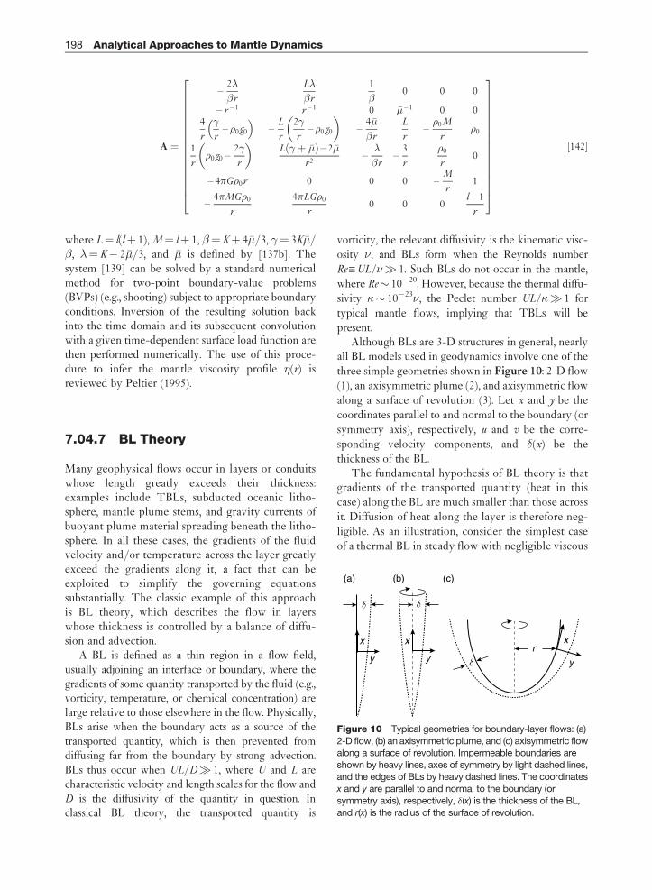
A ¼

–2�

�r

L�

�r

1

�0 0 0

– r – 1 r – 1 0 �� – 1 0 04

r

�

r– �0g0

� �–

L

r

2�

r– �0g0

� �–

4��

�r

L

r–�0M

r�0

1

r�0g0 –

2�

r

� �L � þ ��ð Þ – 2��

r 2–�

�r–

3

r

�0

r0

– 4�G�0r 0 0 0 –M

r1

–4�MG�0

r

4�LG�0

r0 0 0

l – 1

r

26666666666666664

37777777777777775

½142�

where L¼ l(lþ 1), M¼ lþ 1, �¼ Kþ 4��/3, �¼ 3K��/�, �¼ K� 2��/3, and �� is defined by [137b]. Thesystem [139] can be solved by a standard numericalmethod for two-point boundary-value problems(BVPs) (e.g., shooting) subject to appropriate boundaryconditions. Inversion of the resulting solution backinto the time domain and its subsequent convolutionwith a given time-dependent surface load function arethen performed numerically. The use of this proce-dure to infer the mantle viscosity profile �(r) isreviewed by Peltier (1995).

7.04.7 BL Theory

Many geophysical flows occur in layers or conduitswhose length greatly exceeds their thickness:examples include TBLs, subducted oceanic litho-sphere, mantle plume stems, and gravity currents ofbuoyant plume material spreading beneath the litho-sphere. In all these cases, the gradients of the fluidvelocity and/or temperature across the layer greatlyexceed the gradients along it, a fact that can beexploited to simplify the governing equationssubstantially. The classic example of this approachis BL theory, which describes the flow in layerswhose thickness is controlled by a balance of diffu-sion and advection.

A BL is defined as a thin region in a flow field,usually adjoining an interface or boundary, where thegradients of some quantity transported by the fluid (e.g.,vorticity, temperature, or chemical concentration) arelarge relative to those elsewhere in the flow. Physically,BLs arise when the boundary acts as a source of thetransported quantity, which is then prevented fromdiffusing far from the boundary by strong advection.BLs thus occur when UL/D� 1, where U and L arecharacteristic velocity and length scales for the flow andD is the diffusivity of the quantity in question. Inclassical BL theory, the transported quantity is

vorticity, the relevant diffusivity is the kinematic visc-

osity �, and BLs form when the Reynolds number

Re XUL/�� 1. Such BLs do not occur in the mantle,

where Re� 10�20. However, because the thermal diffu-

sivity �� 10�23�, the Peclet number UL/�� 1 for

typical mantle flows, implying that TBLs will be

present.Although BLs are 3-D structures in general, nearly

all BL models used in geodynamics involve one of the

three simple geometries shown in Figure 10: 2-D flow

(1), an axisymmetric plume (2), and axisymmetric flow

along a surface of revolution (3). Let x and y be the

coordinates parallel to and normal to the boundary (or

symmetry axis), respectively, u and v be the corre-

sponding velocity components, and �(x) be the

thickness of the BL.The fundamental hypothesis of BL theory is that

gradients of the transported quantity (heat in this

case) along the BL are much smaller than those across

it. Diffusion of heat along the layer is therefore neg-

ligible. As an illustration, consider the simplest case

of a thermal BL in steady flow with negligible viscous

(a) (b) (c)

δ

δ δ

x x x

y yr

y

Figure 10 Typical geometries for boundary-layer flows: (a)

2-D flow, (b) an axisymmetric plume, and (c) axisymmetric flowalong a surface of revolution. Impermeable boundaries are

shown by heavy lines, axes of symmetry by light dashed lines,

and the edges of BLs by heavy dashed lines. The coordinatesx and y are parallel to and normal to the boundary (or

symmetry axis), respectively, �(x) is the thickness of the BL,

and r(x) is the radius of the surface of revolution.


dissipation of energy. The BL forms of the continuityand energy equations are then

ux þ vy ¼ 0; ½143a�

uTx þ vTy ¼ �Tyy ½143b�

for 2-D flow,

ux þ y – 1 yvð Þy¼ 0 ½144a�

uTx þ vTy ¼ �y – 1 yTy

� �y

½144b�

for an axisymmetric plume, and

ruð Þxþrvy ¼ 0 ½145a�

uTx þ vTy ¼ �Tyy ½145b�

for a surface of revolution. As noted in Section7.04.3.3, the terms uTx and vTy are of the same order.

7.04.7.1 Solution of the BL Equations UsingVariable Transformations

A powerful technique for solving problems involvingBLs is the use of variable transformations to reducethe BL equations to equations of simpler form.One of the most important of these transformationsis that of Von Mises (1927), which transforms the 2-DBL equations into the classical heat conductionequation. A second useful transformation, due toMangler (1948), relates the structure of an axisym-metric BL on a surface of revolution to that of a2-D BL on a flat surface. After introducing bothtransformations, we will show how they can be usedtogether to obtain a solution for the heat transferfrom a hot sphere moving in a viscous fluid(Figure 1(a)).

7.04.7.1.1 Von Mises’s transformation

The essential trick involved in this transformation isto use the streamfunction instead of y as thetransverse coordinate in the BL. Denoting thestreamwise coordinate by a new symbol s X x forclarity, we transform the derivatives in [143b] usingthe chain rule as

qT

qx¼ qT

qs

qs

qxþ qT

q q qx

XqT

qs– v

qT

q ½146�

qT

qy¼ qT

qs

qs

qyþ qT

q q qy

X uqT

q ½147�

where the streamfunction is defined according to theconvention (u, v)¼ ( y, � x). Equation [143b] thenbecomes

qT

qs¼ � q

q uqT

q

� �½148�

Equation [148] takes still simpler forms if thesurface y¼ ¼ 0 is either traction-free or rigid.

Near a free surface, uU(s) is constant across the

BL. Upon introducing a new downstream coordinate

� such that d� ¼U(s)ds, [148] becomes

qT

q�¼ � q

2T

q 2½149�

which is just the classical equation for diffusion of heatin a medium with constant thermal diffusivity �. Theunits of the time-like variable � , however, are nowthose of diffusivity (m2 s�1) rather than of time. Neara rigid surface, u¼ yf (s) and ¼ y2f (s)/2, implyingu (2 f )1/2, where f (s) is arbitrary. Substituting thisresult into [148] and introducing a new downstreamvariable � such that d� ¼ (2f )1/2ds, we obtain

qT

q�¼ � q

q 1=2 qT

q

� �½150�

which describes the diffusion of heat in a mediumwith a position-dependent thermal diffusivity � 1/2

as a function of a time-like variable � having units ofm s�1/2.

Of special interest are the self-similar solutions of[149] and [150] that exist when the wall temperature T0

is constant (¼�T, say) and the upstream temperature

profile is T(0, )¼ 0. The solution of the free-surface

equation [149] has the form T¼�TF(�), where

�¼ /�(�). Separating variables, we obtain �F0/

�F9¼ � _�/�¼�2 (constant), which when solved subject

to the conditions F(0)� 1¼ F(1)¼ �(0)¼ 0 yields

T ¼ �Terfc

2ffiffiffiffiffiffi��p

� �½151�

The solution of the rigid-surface equation [150] hasthe form T¼�TF(�), where � ¼

ffiffiffiffi

p=� �ð Þ.

Separating variables, we find �F0/4�2F9¼ �2 _�/�¼�2 (constant), which when solved subject toF(0)� 1¼ F(1)¼ �(0)¼ 0 with �2¼ 1/3 for conve-nience gives

T

�T¼ 1 –

3

� 1=3ð Þ4

9

� �1=3 Z �

0

exp –4

9x3

� �dx;

� ¼ 1=2

��ð Þ1=3

½152�


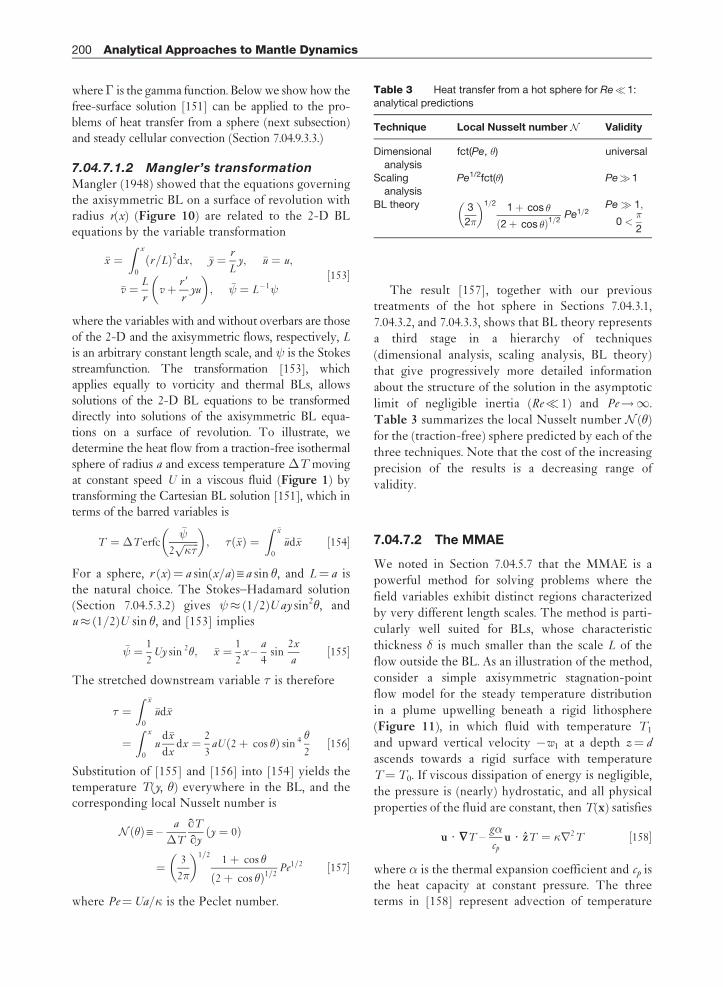
where � is the gamma function. Below we show how thefree-surface solution [151] can be applied to the pro-blems of heat transfer from a sphere (next subsection)and steady cellular convection (Section 7.04.9.3.3.)

7.04.7.1.2 Mangler’s transformation

Mangler (1948) showed that the equations governingthe axisymmetric BL on a surface of revolution withradius r(x) (Figure 10) are related to the 2-D BLequations by the variable transformation

�x ¼Z x

0

r=Lð Þ2dx; �y ¼ r

Ly; �u ¼ u;

�v ¼ L

rv þ r 9

ryu

� �; � ¼ L – 1

½153�

where the variables with and without overbars are thoseof the 2-D and the axisymmetric flows, respectively, L

is an arbitrary constant length scale, and is the Stokesstreamfunction. The transformation [153], whichapplies equally to vorticity and thermal BLs, allowssolutions of the 2-D BL equations to be transformeddirectly into solutions of the axisymmetric BL equa-tions on a surface of revolution. To illustrate, wedetermine the heat flow from a traction-free isothermalsphere of radius a and excess temperature �T movingat constant speed U in a viscous fluid (Figure 1) bytransforming the Cartesian BL solution [151], which interms of the barred variables is

T ¼ �T erfc�

2ffiffiffiffiffiffi��p

� �; � �xð Þ ¼

Z �x

0

�ud�x ½154�

For a sphere, r (x)¼ a sin(x/a) X a sin �, and L¼ a isthe natural choice. The Stokes–Hadamard solution(Section 7.04.5.3.2) gives (1/2)U ay sin2�, andu (1/2)U sin �, and [153] implies

� ¼ 1

2Uy sin 2�; �x ¼ 1

2x –

a

4sin

2x

a½155�

The stretched downstream variable � is therefore

� ¼Z �x

0

�ud�x

¼Z x

0

ud�x

dxdx ¼ 2

3aU 2þ cos �ð Þ sin 4 �

2½156�

Substitution of [155] and [156] into [154] yields thetemperature T(y, �) everywhere in the BL, and thecorresponding local Nusselt number is

N �ð Þ X –a

�T

qT

qyy ¼ 0ð Þ

¼ 3

2�

� �1=21þ cos �

2þ cos �ð Þ1=2Pe1=2 ½157�

where Pe¼Ua/� is the Peclet number.

The result [157], together with our previoustreatments of the hot sphere in Sections 7.04.3.1,

7.04.3.2, and 7.04.3.3, shows that BL theory represents

a third stage in a hierarchy of techniques

(dimensional analysis, scaling analysis, BL theory)

that give progressively more detailed information

about the structure of the solution in the asymptotic

limit of negligible inertia (Re� 1) and Pe!1.

Table 3 summarizes the local Nusselt number N (�)

for the (traction-free) sphere predicted by each of the

three techniques. Note that the cost of the increasing

precision of the results is a decreasing range of

validity.

7.04.7.2 The MMAE

We noted in Section 7.04.5.7 that the MMAE is a

powerful method for solving problems where the

field variables exhibit distinct regions characterized

by very different length scales. The method is parti-

cularly well suited for BLs, whose characteristic

thickness � is much smaller than the scale L of the

flow outside the BL. As an illustration of the method,

consider a simple axisymmetric stagnation-point

flow model for the steady temperature distribution

in a plume upwelling beneath a rigid lithosphere

(Figure 11), in which fluid with temperature T1

and upward vertical velocity �w1 at a depth z¼ d

ascends towards a rigid surface with temperature

T¼T0. If viscous dissipation of energy is negligible,

the pressure is (nearly) hydrostatic, and all physical

properties of the fluid are constant, then T(x) satisfies

u ? �T –g

cp

u ? zT ¼ �r2T ½158�

where is the thermal expansion coefficient and cp isthe heat capacity at constant pressure. The threeterms in [158] represent advection of temperature

Table 3 Heat transfer from a hot sphere for Re� 1:

analytical predictions

Technique Local Nusselt number N Validity

Dimensional

analysis

fct(Pe, �) universal

Scaling

analysis

Pe1/2fct(�) Pe�1

BL theory 3

2�

� �1=2 1þ cos �

2þ cos �ð Þ1=2Pe1=2

Pe� 1;

0 <�

2


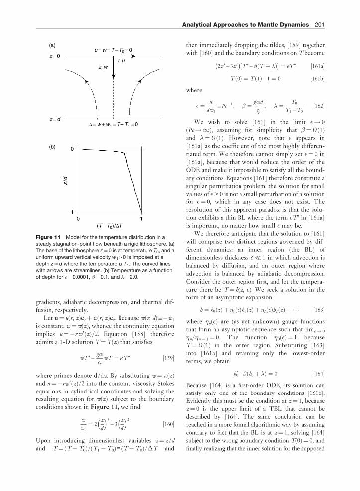
gradients, adiabatic decompression, and thermal dif-fusion, respectively.

Let u¼ u(r, z)erþw(r, z)ez. Because w(r, d) X�w1

is constant, w¼w(z), whence the continuity equationimplies u¼�r w9(z)/2. Equation [158] thereforeadmits a 1-D solution T¼T(z) that satisfies

wT 9 –g

cp

wT ¼ �T 0 ½159�

where primes denote d/dz. By substituting w¼w(z)and u¼�rw9(z)/2 into the constant-viscosity Stokesequations in cylindrical coordinates and solving theresulting equation for w(z) subject to the boundaryconditions shown in Figure 11, we find

w

w1¼ 2

z

d

� �3

– 3z

d

� �2

½160�

Upon introducing dimensionless variables z¼ z/d

and T¼ (T�T0)/(T1�T0) X (T�T0)/�T and

then immediately dropping the tildes, [159] togetherwith [160] and the boundary conditions on T become

2z3 – 3z2� �

T 9 –� T þ �ð Þ½ � ¼ T 0 ½161a�

T 0ð Þ ¼ T 1ð Þ – 1 ¼ 0 ½161b�

where

¼ �

dw1XPe – 1; � ¼ gd

cp

; � ¼ T0

T1 –T0½162�

We wish to solve [161] in the limit ! 0(Pe!1), assuming for simplicity that �¼O (1)and �¼O (1). However, note that appears in[161a] as the coefficient of the most highly differen-tiated term. We therefore cannot simply set ¼ 0 in[161a], because that would reduce the order of theODE and make it impossible to satisfy all the bound-ary conditions. Equations [161] therefore constitute asingular perturbation problem: the solution for smallvalues of > 0 is not a small perturbation of a solutionfor ¼ 0, which in any case does not exist. Theresolution of this apparent paradox is that the solu-tion exhibits a thin BL where the term T0 in [161a]is important, no matter how small may be.

We therefore anticipate that the solution to [161]will comprise two distinct regions governed by dif-ferent dynamics: an inner region (the BL) ofdimensionless thickness �� 1 in which advection isbalanced by diffusion, and an outer region whereadvection is balanced by adiabatic decompression.Consider the outer region first, and let the tempera-ture there be T¼ h(z, ). We seek a solution in theform of an asymptotic expansion

h ¼ h0 zð Þ þ �1 ð Þh1 zð Þ þ �2 ð Þh2 zð Þ þ � � � ½163�

where �n( ) are (as yet unknown) gauge functionsthat form an asymptotic sequence such that lim ! 0

�n/�n� 1¼ 0. The function �0( )¼ 1 becauseT¼O (1) in the outer region. Substituting [163]into [161a] and retaining only the lowest-orderterms, we obtain

h90 –� h0 þ �ð Þ ¼ 0 ½164�

Because [164] is a first-order ODE, its solution cansatisfy only one of the boundary conditions [161b].Evidently this must be the condition at z¼ 1, becausez¼ 0 is the upper limit of a TBL that cannot bedescribed by [164]. The same conclusion can bereached in a more formal algorithmic way by assumingcontrary to fact that the BL is at z¼ 1, solving [164]subject to the wrong boundary condition T(0)¼ 0, andfinally realizing that the inner solution for the supposed

0

10 1

(a)

(b)

z = 0r, u

z, wz

/d

z = du = w + w1 = T – T1 = 0

(T – T0) /ΔT

u = w = T – T0 = 0

Figure 11 Model for the temperature distribution in a

steady stagnation-point flow beneath a rigid lithosphere. (a)The base of the lithosphere z¼ 0 is at temperature T0, and a

uniform upward vertical velocity w1 > 0 is imposed at a

depth z¼d where the temperature is T1. The curved lines

with arrows are streamlines. (b) Temperature as a functionof depth for ¼ 0.0001, �¼ 0.1. and �¼ 2.0.


BL is unphysical because it increases exponentiallyupward. The lowest-order terms of the (correct)boundary condition are h0(1)¼ 1, and the solution of[164] that satisfies this is

h0 ¼ 1þ �ð Þ exp � z – 1ð Þ –� ½165�

Turning now to the inner region, the first task is todetermine which term on the LHS of [161a] balancesthe RHS. Suppose (contrary to fact, as will soonappear) that �(Tþ�)�T 9 (decompression�advection). Because z� � and z2� z3 in the BL, thebalance z2�(Tþ�)� T0 implies �� 1/4. But thenT 9��(Tþ�), which contradicts our original

assumption. The correct balance must therefore bez2T 9� T0 (advection� diffusion), which implies�� 1/3 and T 9��(Tþ�), consistent with ouroriginal assumption. A more physical argument thatleads to the same conclusion is to note that the

vertical scale length over which adiabatic decom-pression is significant in the mantle (�1000 km) ismuch greater than a typical BL thickness.

Now that we know the thickness of the BL, we canproceed to determine its structure. To discern thethin BL distinctly, we use a sort of mathematicalmagnifying glass: a new stretched depth coordinatez¼ z/� X z �1/3 that is of order unity in the BL.

Denoting the inner solution by f (z, ) and writing[161a] in terms of z, we find

2 z3 – 3 2=3z2� �

– 1=3f 9 – � f þ �ð Þh i

¼ 1=3f 0 ½166�

where primes denote differentiation with respect to z.We now seek a solution in the form

f ¼ f0 zð Þ þ �1 ð Þf1 zð Þ þ �2 ð Þf2 zð Þ þ � � � ½167�

where �n( ) are unknown gauge functions.Substituting [167] into [166] and retaining only thelowest-order terms, we obtain

f 00 þ 3z2f 90 ¼ 0 ½168�

The solution of [168] that satisfies the boundarycondition f0(0)¼ 0 is

f0 ¼ A

Z z

0

exp –x3� �

dx XA

3� 1=3; z3� �

½169�

where � a; xð Þ ¼R x

0 exp – tð Þt a – 1dt is the incom-plete Gamma function and A is an unknownconstant that must be determined by matching[169] to the outer solution [165].

The most rigorous way to do the matching is torewrite both the inner and outer expansions in terms

of an intermediate variable zint¼ �( )z such that �1/3� �� 1, and then to choose the values ofany unknown constants (A in this case) so that thetwo expressions agree. However, it is often possibleto use a simpler matching principle, due to Prandtl,which states that the inner limit of the outer expan-sion must be equal to the outer limit of the innerexpansion – roughly speaking, that the two expan-sions must match at the edge of the BL. For ourproblem, Prandtl’s principle is

limz!1

f0 zð Þ ¼ limz!0

h0 zð Þ; whence

A ¼ 3 1þ �ð Þ exp –�ð Þ –�½ �� 1=3ð Þ

½170�

where � is the Gamma function.The last step is to construct a composite expan-

sion that is valid both inside and outside the BL. Thisis just the sum of the inner and outer expansions lesstheir shared common part h0(z! 0), or

T ¼ h0 zð Þ þ 1þ �ð Þexp – �ð Þ –�½ � � 1=3; z3= ð Þ� 1=3ð Þ – 1

� �

½171�

The procedure described above is a first-ordermatching that retains only the first terms in the expan-sions [163] and [167]. If desired, the matching can becarried out to higher order by working back and forthbetween the inner and outer expansions, determiningthe gauge functions �n( ) and �n( ) and matching at eachstep. Higher-order matching often requires the use ofthe more rigorous intermediate matching principle; forexamples see Hinch (1991), Kevorkian and Cole (1996),or the somewhat less formal treatments of Nayfeh(1973) or Van Dyke (1975). For many problems, how-ever, first-order matching suffices to reveal the essentialstructure and physical significance of the solution.

The MMAE has been used to solve a variety ofgeophysically relevant problems involving BLs,mostly with constant viscosity. Umemura and Busse(1989) studied the axisymmetric convective flow in acylindrical container of height d with free-slipboundaries, using the MMAE to match the interiorflow to the central rising plume and the circumfer-ential downwelling. They found that the verticalvelocity in the plume is w� (�/d)(�ln )1/2Ra2/3,where the dimensionless plume radius X a/d satis-fies (�ln )1/4� Ra�1/6, Ra� 1 being the Rayleighnumber. Whittaker and Lister (2006a) studied creep-ing plumes from a point heat source with buoyancyflux B on an impermeable plane boundary by match-ing the BL flow to an outer flow that sees the plume


as a line distribution of Stokeslets. They found thatthe vertical velocity w� (B/�)1/2[ln(z/z0)]1/2, wherez is the height and z0¼ 32��2�/B. Whittaker andLister (2006b) studied the dynamics of a plumeabove a heated disk on a plane boundary, and usedthe MMAE to match the flow within the plume toboth an outer flow and a horizontal BL flow acrossthe disk. The results show that the Nusselt numberN� Ra1/5 for a rigid boundary and N� (Ra/ln Ra)1/3

for a free-slip boundary, where Ra� 1 is definedusing the disk radius. An application of the MMAEto a problem with variable viscosity (Morris, 1982)appears in the next subsection.

7.04.7.3 BLs with Strongly VariableViscosity

In a fluid with constant viscosity and infinite Prandtlnumber, thermal BLs are not accompanied by vorti-city BLs, because the velocity field varies on a lengthscale much larger than the thickness of the TBL. As aresult, the velocity field within the BL can be repre-sented by the first term of its Taylor series expansion(or its multipole expansion in the case of an axisym-metric plume; cf. Whittaker and Lister, 2006a), whichgreatly simplifies the task of solving the thermal BLequation. This happy state of affairs no longer obtainsif the viscosity of the fluid depends on temperature,because the velocity and temperature fields are thencoupled.

Most studies of variable-viscosity BLs in the geo-dynamics literature focus on mantle plumes in eitherplanar (Figure 10(a)) or axisymmetric (Figure 10(b))geometry. The basic procedure is to supplement theBL equations [143] or [144] with a simplified BL formof the vertical component of the momentum equationin which derivatives along the BL are neglected rela-tive to those normal to it. In physical terms, thisequation simply states that the buoyancy force in theplume is balanced by the lateral gradient of the ver-tical shear stress � , or

y – nqy yn�ð Þ þ �g T –T1ð Þ ¼ 0 ½172�

where T1 is the temperature far from the plume, y isthe coordinate normal to the plume, and n¼ 0 or 1for planar or axisymmetric geometries, respectively.

An important early study based on [172] in planargeometry was that of Yuen and Schubert (1976), whoinvestigated the buoyant upwelling adjacent to a ver-tical, isothermal, and traction-free plane of a fluidwith temperature-dependent Newtonian or power-

law rheology. The governing BL equations governingadmit a similarity transformation of the form

T ¼T1 þ f �ð Þ; ¼ x nþ2ð Þ= nþ3ð Þg �ð Þ;� ¼ yx – 1= nþ3ð Þ ½173�

where is the streamfunction and n is the power-lawexponent. The more realistic case of an axisymmetricplume from a point source of heat in a fluid withtemperature-dependent viscosity was studied byMorris (1980), Loper and Stacey (1983), and Olsonet al. (1993). Using a similarity transformation, Morris(1980) found that the temperature on the plume axisdecreases exponentially upward with a scale heightQ/12�kc�Tr, where Q is the total heat flux carried bythe plume, �Tr is the temperature change requiredto change the viscosity by a factor e, and kc is thethermal conductivity. Using a simpler approach inwhich the functional form of the temperature profileacross the plume is assumed, Olson et al. (1993) founda scale height equal to three times that determined byMorris (1980). Hauri et al. (1994) considered a similarproblem, but with an empirical superexponentialtemperature- and depth-dependent viscosity law.

While plumes involve free or buoyancy-driven con-vection, variable-viscosity BLs can also arise insituations where a large-scale background flow orwind is imposed externally (forced convection). Anexample is the previously introduced stagnation-pointflow model for the heat transfer from a hot spheremoving in a fluid with strongly temperature-dependentviscosity (Figure 1(b)). Using the MMAE, Morris(1982) showed that three distinct dynamical regimesoccur: a conduction limit; a Stokes limit in which theflow around the sphere resembles that in an isoviscousfluid; and a lubrication limit in which most of thevolume flux is carried by the low-viscosity BL adjoin-ing the hot plate. Solutions in spherical geometry wereobtained by Morris (1982) and Ansari and Morris(1985) for the lubrication limit and an intermediate(lubrication/Stokes) limit.

7.04.8 Long-Wave Theories

Long-wave theories comprise a variety of looselyrelated approaches whose goal is to describe theevolving thickness or shape of a thin layer. Thefundamental idea underlying these approaches isthe distinction between small amplitude and smallslope. To take a simple example, if a 2-D fluid layerhas thickness h0þ�h sin kx, its surface has small


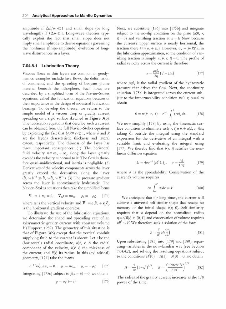
amplitude if �h/h0� 1 and small slope (or longwavelength) if k�h� 1. Long-wave theories typi-cally exploit the fact that small slope does notimply small amplitude to derive equations governingthe nonlinear (finite-amplitude) evolution of long-wave disturbances in a layer.

7.04.8.1 Lubrication Theory

Viscous flows in thin layers are common in geody-namics: examples include lava flows, the deformationof continents, and the spreading of buoyant plumematerial beneath the lithosphere. Such flows aredescribed by a simplified form of the Navier–Stokesequations, called the lubrication equations because oftheir importance in the design of industrial lubricationbearings. To develop the theory, we return to thesimple model of a viscous drop or gravity currentspreading on a rigid surface sketched in Figure 3(b).The lubrication equations that describe such a currentcan be obtained from the full Navier–Stokes equationsby exploiting the fact that h/RX � 1, where h and R

are the layer’s characteristic thickness and lateralextent, respectively. The thinness of the layer hasthree important consequences: (1) The horizontalfluid velocity u X uexþ vey along the layer greatlyexceeds the velocity w normal to it. The flow is there-fore quasi-unidirectional, and inertia is negligible. (2)Derivatives of the velocity components across the layergreatly exceed the derivatives along the layer(qz� h�1� qx� qy� R�1). (3) The pressure gradientacross the layer is approximately hydrostatic. TheNavier–Stokes equations then take the simplified forms

�1 ? uþ wz ¼ 0; �1p ¼ �uzz; pz ¼ – �g ½174�

where w is the vertical velocity and �1¼ exqxþ eyqy

is the horizontal gradient operator.To illustrate the use of the lubrication equations,

we determine the shape and spreading rate of anaxisymmetric gravity current with constant volumeV (Huppert, 1982). The geometry of this situation isthat of Figure 3(b) except that the vertical conduitsupplying fluid to the current is absent. Let r be the(horizontal) radial coordinate, u(z, r, t) the radialcomponent of the velocity, h(r, t) the thickness ofthe current, and R(t) its radius. In this (cylindrical)geometry, [174] take the forms

r – 1 ruð Þrþwz ¼ 0; pr ¼ �uzz; pz ¼ – �g ½175�

Integrating [175c] subject to p(z¼ h)¼ 0, we obtain

p ¼ �g h – zð Þ ½176�

Next, we substitute [176] into [175b] and integratesubject to the no-slip condition on the plate (u(0, r,t)¼ 0) and vanishing traction at z¼ h. Now becausethe current’s upper surface is nearly horizontal, thetraction there �(uzþwx). However, wx� (h/R)2uz inthe lubrication approximation, so the condition of van-ishing traction is simply uz(h, r, t)¼ 0. The profile ofradial velocity across the current is therefore

u ¼ �ghr

2�z2 – 2hz� �

½177�

where �ghr is the radial gradient of the hydrostaticpressure that drives the flow. Next, the continuityequation [175a] is integrated across the current sub-ject to the impermeability condition w(0, r, t)¼ 0 toobtain

0 ¼ w h; r ; tð Þ þ r – 1

Z h

0

ruð Þr dz ½178�

We now simplify [178] by using the kinematic sur-face condition to eliminate w(h, r, t) X htþ u(h, r, t)hr;taking qr outside the integral using the standardexpression for the derivative of an integral with avariable limit; and evaluating the integral using[177]. We thereby find that h(r, t) satisfies the non-linear diffusion equation

ht ¼ 4�r – 1 rh3hr

� �r; � ¼ �g

12�½179�

where � is the spreadability. Conservation of thecurrent’s volume requires

2�

Z R

0

rh dr ¼ V ½180�

We anticipate that for long times, the current willachieve a universal self-similar shape that retains no

memory of the initial shape h(r, 0). Self-similarityrequires that h depend on the normalized radius� X r/R(t) P [0, 1], and conservation of volume requireshR2�V. We therefore seek a solution of the form

h ¼ V

R2H

r

R

� �½181�

Upon substituting [181] into [179] and [180], separ-ating variables in the now-familiar way (see Section7.04.4.2), and solving the resulting equations subjectto the conditions H9(0)¼H(1)¼ R(0)¼ 0, we obtain

H ¼ 4

3�1 – �2� �1=3

; R ¼ 4096�V 3t

81�3

� �1=8

½182�

The radius of the gravity current increases as the 1/8power of the time.


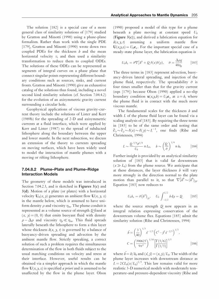
The solution [182] is a special case of a moregeneral class of similarity solutions of [179] studiedby Gratton and Minotti (1990) using a phase-planeformalism. Rather than work with the single PDE[179], Gratton and Minotti (1990) wrote down twocoupled PDEs for the thickness h and the meanhorizontal velocity v, and then used a similaritytransformation to reduce them to coupled ODEs.The solutions of these ODEs can be represented assegments of integral curves on a phase plane thatconnect singular points representing different bound-ary conditions such as sources, sinks, and currentfronts. Gratton and Minotti (1990) give an exhaustivecatalog of the solutions thus found, including a novelsecond kind similarity solution (cf. Section 7.04.4.2)for the evolution of an axisymmetric gravity currentsurrounding a circular hole.

Geophysical applications of viscous gravity-cur-rent theory include the solutions of Lister and Kerr(1989b) for the spreading of 2-D and axisymmetriccurrents at a fluid interface, which were applied byKerr and Lister (1987) to the spread of subductedlithosphere along the boundary between the upperand lower mantle. In the next subsection, we discussan extension of the theory to currents spreadingon moving surfaces, which have been widely usedto model the interaction of mantle plumes with amoving or rifting lithosphere.

7.04.8.2 Plume–Plate and Plume–RidgeInteraction Models

The geometry of these models was introduced inSection 7.04.2.3, and is sketched in Figures 3(c) and3(d). Motion of a plate (or plates) with a horizontalvelocity U0(x, y) generates an ambient flow U(x, y, z)in the mantle below, which is assumed to have uni-form density � and viscosity �m. The plume conduit isrepresented as a volume source of strength Q fixed at(x, y)¼ (0, 0) that emits buoyant fluid with density�� and viscosity �p� �m. This fluid spreadslaterally beneath the lithosphere to form a thin layerwhose thickness h(x, y, t) is governed by a balance ofbuoyancy-driven spreading and advection by theambient mantle flow. Strictly spreaking, a correctsolution of such a problem requires the simultaneousdetermination of the flow in both fluids subject to theusual matching conditions on velocity and stress attheir interface. However, useful results can beobtained via a simpler approach in which the mantleflow U(x, y, z) is specified a priori and is assumed to beunaffected by the flow in the plume layer. Olson

(1990) proposed a model of this type for a plumebeneath a plate moving at constant speed U0

(Figure 3(c)), and derived a lubrication equation forh(x, y, t) assuming a uniform mantle flowU(x,y,z)¼U0ex . For the important special case of asteady-state plume layer, the lubrication equation is

U0hx ¼ ��r21h4 þ Q � xð Þ� yð Þ; �� ¼ ��g

48�p½183�

The three terms in [183] represent advection, buoy-ancy-driven lateral spreading, and injection of theplume fluid, respectively. The spreadability �� isfour times smaller than that for the gravity current(eqn [179]) because Olson (1990) applied a no-slipboundary condition u(x,y,h)¼U0ex at z¼ h, wherethe plume fluid is in contact with the much moreviscous mantle.

The fundamental scales for the thickness h andwidth L of the plume fluid layer can be found via ascaling analysis of [183]. By requiring the three termsin [183] to be of the same order and noting thatqx� qy� �(x)� �( y)� L�1, one finds (Ribe andChristensen, 1994)

L � Q 3=4 ��1=4

U0XL0; h � Q

��

� �1=4

X h0 ½184�

Further insight is provided by an analytical similaritysolution of [183] that is valid far downstream(x� L0) from the plume source. We anticipate thatat these distances, the layer thickness h will varymore strongly in the direction normal to the platemotion than parallel to it, so that r1

2h4� (h4)yy.Equation [183] now reduces to

U0hx ¼ �� h4� �

yy; U0

Z L=2

– L=2

h dy ¼ Q ½185�

where the source strength Q now appears in anintegral relation expressing conservation of thedownstream volume flux. Equations [185] admit thesimilarity solution (Ribe and Christensen, 1994)

h ¼ 3

40

� �1=3

x – 1=5 C2 – y2x – 2=5� �1=3

;

C ¼ 390625

9�3

� �1=10 � 5=6ð Þ� 1=3ð Þ

� �3=5

½186�

where h¼ h/h0 and (x, y)¼ (x, y)/L0. The width of theplume layer increases with downstream distance asL¼ 2CL0(x/L0)1/5. This law remains valid for morerealistic 3-D numerical models with moderately tem-perature-and pressure-dependent viscosity (Ribe and


Christensen, 1994, 1999), but must eventually breakdown if the mantle/plume viscosity contrast becomestoo large.

The interaction of a plume with an oceanicspreading ridge has been studied using a modifiedversion of Olson’s (1990) model in which the uniformmantle flow U¼U0ex is replaced by a cornerflow driven by surface plates diverging with a half-spreading rate U0 (Figure 3(d); Ribe et al., 1995). Thebalance of the source term Q�(x)�( y) with verticaladvection directly beneath the ridge yields a newlength scale L1� (Q/U0)1/2, which agrees well withthe along-strike extent of the plume fluid beneath theridge (waist width) determined by laboratory experi-ments (Feighner and Richards, 1995) and numericalmodels (Ribe et al., 1995.)

An important extension of the theory for geody-namical applications is to currents in which both thebuoyancy and viscosity depend on temperature. Sucha theory was developed by Bercovici (1994) andBercovici and Lin (1996), who supplemented theusual lubrication theory equations with an energyequation describing the temperature distributioninside the current. They found that variable viscosityand buoyancy strongly influence the current’s shapeand spreading rate, which typically no longer exhibitthe self-similar behavior typical of currents with con-stant properties.

7.04.8.3 Long-Wave Analysis of BuoyantInstability

In convecting systems such as the Earth’s mantle,plumes arise as instabilities of horizontal TBLs. Along-wave model for this process has been proposedby Lemery et al. (2000; henceforth LRS00), based ontwo assumptions: that the wavelength of the initialinstability greatly exceeds the BL thickness, and thatthe horizontal velocity of the fluid is approximatelyconstant across the BL. These assumptions allow thecoupled 3-D dynamics of the BL and the fluid out-side it to be reduced to 2-D equations for the lateralvelocity at the edge of the BL and a temperaturemoment that describes the distribution of buoyancywithin it.

The domain of the model is a fluid half-spacebounded by a cold traction-free surface x3¼ 0 heldat temperature ��T relative to the fluid far from it(Figure 2(b)) The BL occupies the depth intervalx3 < h(x1, x2, t), where x are Cartesian coordinatesparallel to the BL and t is time. In the following,hatted and unhatted variables are those in the BL

and in the interior, respectively, and an argument in

parentheses indicates a value of x3. The (constant)

viscosity of the outer fluid is �0, and the viscosity

within the BL is �(x3).The starting point is the momentum equation

within the BL, namely, �qipþ qj�ij¼ �0gT�i3,

where �ij is the deviatoric part of the stress tensor.

Taking the curl of this equation, applying the con-

tinuity equation �33¼��, and noting that (q112 �3,

q122 �3, q22

2 �3)� q33�3 in the long-wavelength

approximation, we obtain

q233�3þ q3A ¼ –�0gqT; A ¼ q�� þ q� �� ½187�

Physically, [187] are the lateral (¼ 1 or 2) compo-nents of the vorticity equation. Now multiply [187]by x3, integrate across the BL from x3¼ 0 to x3¼ h,and take lateral derivatives outside the integral signsby neglecting the small lateral variation of the upperlimit h(x1, x2, t). The result is

– �3 hð Þ þ hq3�3 hð Þ þ hA hð Þ – A� �

¼ �0gqM

½188�

where hi ¼R h

0 dx3 and

M ¼ – x3T� �

½189�

is the temperature moment. Now h q3�3(h)� �3(h)in the long-wave limit, and continuity of shear stressat x3¼ h requires �3(h)¼ �3(h). But because theinterior fluid sees the BL as a skin with zero thick-ness, �3(h) �3(0) �0q3u(0). Moreover, thelateral velocity components are constant across thelayer to lowest order and must match those in theinterior fluid, requiring u¼ u(0) and ��¼�(x3)[qu�(0)þ q�u(0)]. Substituting these expres-sions into [188], we find

–q3u–� ? � 2e– I� ? uð Þ½ �–� 3�� ? uð Þ ¼ �0g

�0�M ½190�

where

� ¼ � x3ð Þ – �0

�0

� �½191�

is a relative excess surface viscosity, u is the horizon-tal velocity vector, e is the 2-D strain-rate tensor, � isthe 2-D gradient operator, I is the identity tensor,and all terms are evaluated at x3¼ 0. Equation [191]is an effective boundary condition that representsthe influence of the BL on the interior fluid. Itshows that the BL acts like an extensible skin withshear viscosity ��0 and compressional viscosity 3��0

that applies a shear stress proportional to �M to theouter fluid.


The next step is to determine explicitly the flowin the outer fluid that is driven by lateral variations inM by solving the Stokes equations in the half-spacex3� 0 subject to [190]. Evaluating the resulting solu-tion at x3¼ 0, we obtain the closure relationship(LRS00, eqn [2.41])

�u kð Þ ¼ ik

2k 1þ 2�kð Þ�0g

�0

�M kð Þ ½192�

where k is the horizontal wave vector, k¼ jkj, andoverbars denote the Fourier transform. Equation [192]is only valid if � does not vary laterally. Finally, anevolution equation for M is obtained by taking the firstmoment of the energy equation, yielding

qt M þ u ? �M þ 2M� ? u ¼ � r2M þ�T� �

½193�

Equations [192] and [193] are three equations foru(x1, x2, t) and M(x1, x2, t) that can be solved numeri-cally subject to periodic boundary conditions in thelateral directions for a specified initial conditionM(x1, x2, 0).

An important special case of the aboveequations is the R–T instability of a layer with den-sity �0þ�� and viscosity �1¼ ��0, obtained by thetransformation

M ! h2��=2�0; �! h � – 1ð Þ; �! 0 ½194�

A linear stability analysis of [192] and [193] can nowbe performed by setting h¼ h0þ h exp(ik ? x) exp(st)and u¼ u exp(ik ? x) exp (st) and linearizing in theperturbations h and u. The resulting growth rateis s/s1¼ �/2[1þ 2 (�� 1)], where ¼ h0k ands1 ¼ g��h0=�1, which agrees with the exact analy-

tical expression [29] if �� . Equations [190]–[193]are therefore valid as long as the BL is not too muchless viscous than the outer fluid.

The above equations also describe the finite-amplitude evolution of the R–T instability of adense viscous layer over a passive half-space(Canright and Morris, 1993 XCM93). Because thehalf-space is effectively inviscid (�!1), the closurelaw (192) is not meaningful, and the relevant equa-tions are [190] and [193]. Rewriting these using [194]and noting that the first term in [190] (shear stressapplied by the inviscid fluid) is negligible, we obtain

�g��

4�1h2 þ h� ? u

� �þ � ? heð Þ ¼ 0 ½195�

qt h þ � ? huð Þ ¼ 0 ½196�

which are just the dimensional forms of eqns [3.8] and[3.7], respectively, of CM93.

A remarkable feature of the eqns [192]–[193] and[195]–[196] is the existence of similarity solutions inwhich M or h becomes infinite at a finite time ts,corresponding to the runaway escape of the plumefrom its source layer. The general form of the solu-tion for h or M1/2 is

h or M1=2 ¼ ts – tð Þafctx

ts – tð Þb

!½197�

where x is the lateral or radial distance from the peakof the instability and a and b are exponents. CM93’ssolution of [195]–[196] gives a¼�1 for a Newtonianfluid, whereas LRS00 solved [192]–[193] in the limit�� 1 to find a¼�1/2. The discrepancy appears tobe due to the fact that LRS00 treated � as a constant,whereas � _ h in the problem studied by CM93.

7.04.8.4 Theory of Thin Shells, Plates, andSheets

A central problem in geodynamics is to determinethe response of the lithosphere to applied loads suchas seamounts, plate boundary forces (ridge push, slabpull, etc.), and tractions imposed by underlyingmantle convection. Such problems can be solvedeffectively using thin-shell theory, a branch ofapplied mechanics concerned with the behavior ofsheet-like objects whose thickness h is much smallerthan their typical radius of curvature R. This condi-tion is evidently satisfied for the Earth’s lithosphere,for which h 100 km and R 6300 km. A furtherassumption of thin-shell theory is that the stresseswithin the shell vary laterally on a length scale L� h.Thin-shell theory therefore properly belongs to thegeneral class of long-wave theories.

The basic idea of thin-shell theory is to exploit thesmallness of h/R to reduce the full 3-D dynamicalequations to equivalent 2-D equations for thedynamics of the shell’s mid-surface. Let the 3-DCartesian coordinates of any point on this surfacebe x0(�1, �2), where � are coordinates on the mid-surface itself. In the most general formulations ofshell theory (e.g., Niordson, 1985), � are allowed tobe arbitrary and nonorthogonal. Such a formulation isuseful for problems involving large finite deforma-tion, because � can be treated as Lagrangiancoordinates. If the deformation is small, however, itmakes sense to define � as orthogonal lines-of-curvature coordinates whose isolines are parallel tothe two directions of principal curvature of the mid-surface at each point. This less elegant but more


readily understandable formulation is the one used inmost geodynamical applications of shell theory.

Relative to lines-of-curvature coordinates, thefundamental quantities that describe the shape ofthe mid-surface are the principal radii ofcurvature R and the Lame parameters A¼ jqx0j,where q¼ q/q�. For notational convenience, letB¼ 1/A and K¼ 1/R. All vector and tensorquantities defined on the mid-surface are expressedrelative to a local orthonormal basis comprising twosurface-parallel unit vectors d1, d2 and a normalvector d3 defined by

d1 ¼ B1q1x0; d2 ¼ B2q2x0; d3 ¼ d1 � d2 ½198�

In the following, z is a coordinate normal to the mid-surface z¼ 0. Moreover, the repeated subscript isnot summed unless explicitly indicated, and �¼ 2when ¼ 1 and vice versa.

The general equilibrium equations for a shellwithout inertia are (Novozhilov, 1959, p. 39)

q A�T

� �þ q� ASð Þ þ Sq�A –T�qA�

þ Kq A�M

� �–M�qA�

þ 2q� AHð Þ þ 2RK�Hq�A¼ – A1A2P ½199a�

X2

¼1

�B1B2q

B�q A�M

� �–M�qA�

þ q� AHð Þ þ Hq�A�

–KT

�¼ – P3 ½199b�

where

T ¼Z h=2

– h=2

1þ K�z� �

�dz;

S ¼Z h=2

– h=2

1 –K1K2z2� �

�12dz ½200a�

M ¼Z h=2

– h=2

z 1þ K�z� �

�dz;

H ¼Z h=2

– h=2

z 1þ K1 þ K2ð Þz=2½ ��12dz ½200b�

Pi is the total load vector (per unit midsurface area),and �� is the usual Cauchy stress tensor. The essen-tial content of [199] is that a loaded shell can deformin two distinct ways: by in-plane stretching and shear,the intensity of which is measured by the stressresultants T and S, and by bending, which is mea-sured by the bending moments M and H. In generalboth modes are present, in a proportion that dependsin a complicated way on the mid-surface shape.Shells that deform only by extension and in-planeshear (M¼H¼ 0) are called membranes.

Equations [199] are valid for a shell of any mate-rial. To solve them, we need constitutive relationsthat link T, S, M, and H to the displacement vi (foran elastic shell) or the velocity ui (for a fluid shell) ofthe mid-surface. For an elastic shell with Young’smodulus E and Poisson’s ratio �, these are(Novozhilov, 1959, pp. 24, 48)

T ¼Eh

1 – �2 þ � ��

;

MEh3

12 1 –�2ð Þ � þ ��

½201a�

S ¼ Eh

2 1þ �ð Þ!; H ¼ Eh3

12 1þ �ð Þ � ½201b�

where

¼ Bqva þ B1B2v�q�A þ Kv3 ½202a�

! ¼X2

¼1

A�Bq B�v��

½202b�

� ¼ – Bq Bqv3 –Kvð Þ– B1B2q�A B�q�v3 –K�v�

� �½202c�

� ¼ – B1B2q212u3 þ

X2

¼1

B1B2B q�A� �

qv3

�

þK B�q�v – B1B2u3q�A� ��

½202d�

are the six independent quantities that describethe deformation of the mid-surface: the elongations and the changes of curvature � in the twocoordinate directions, the in-plane shear deformation!, and the torsional (twist) deformation � . Theanalogous expressions for a fluid shell are obtainedby applying the transformation [135] to [201] and[202].

The above equations include all the special casescommonly considered in geodynamics. The first isthat of a flat (R1¼ R2¼1, A1¼ A2¼ 1) elastic platewith constant thickness h. The (uncoupled) equationsgoverning the flexural and membrane modes are(Landau and Lifshitz, 1986)

Eh3

12 1 – �2ð Þr41v3 ¼ P3 ½203a�

Eh

2 1 – �2ð Þ 1 – �ð Þr2vþ 1þ �ð Þ� � ? vð Þ

¼ –P1e1 –P2e2

½203b�

where r2, �, and v are the 2D (in-plane) Laplacianoperator, gradient operator, and displacement vector,


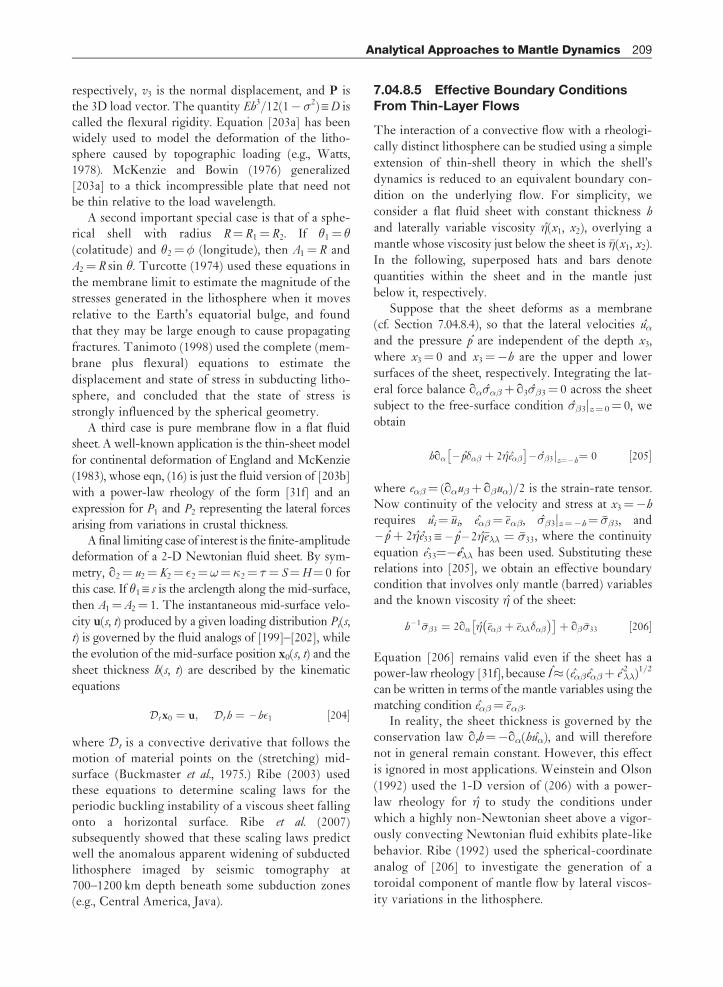
respectively, v3 is the normal displacement, and P isthe 3D load vector. The quantity Eh3/12(1� �2) XD iscalled the flexural rigidity. Equation [203a] has beenwidely used to model the deformation of the litho-sphere caused by topographic loading (e.g., Watts,1978). McKenzie and Bowin (1976) generalized[203a] to a thick incompressible plate that need notbe thin relative to the load wavelength.

A second important special case is that of a sphe-rical shell with radius R¼ R1¼ R2. If �1¼ �(colatitude) and �2¼� (longitude), then A1¼ R and

A2¼ R sin �. Turcotte (1974) used these equations in

the membrane limit to estimate the magnitude of thestresses generated in the lithosphere when it moves

relative to the Earth’s equatorial bulge, and found

that they may be large enough to cause propagating

fractures. Tanimoto (1998) used the complete (mem-

brane plus flexural) equations to estimate the

displacement and state of stress in subducting litho-

sphere, and concluded that the state of stress is

strongly influenced by the spherical geometry.A third case is pure membrane flow in a flat fluid

sheet. A well-known application is the thin-sheet model

for continental deformation of England and McKenzie

(1983), whose eqn, (16) is just the fluid version of [203b]

with a power-law rheology of the form [31f] and an

expression for P1 and P2 representing the lateral forcesarising from variations in crustal thickness.

A final limiting case of interest is the finite-amplitudedeformation of a 2-D Newtonian fluid sheet. By sym-

metry, q2¼ u2¼ K2¼ 2¼!¼�2¼ � ¼ S¼H¼ 0 for

this case. If �1X s is the arclength along the mid-surface,

then A1¼ A2¼ 1. The instantaneous mid-surface velo-

city u(s, t) produced by a given loading distribution Pi(s,

t) is governed by the fluid analogs of [199]–[202], while

the evolution of the mid-surface position x0(s, t) and the

sheet thickness h(s, t) are described by the kinematic

equations

D t x0 ¼ u; D t h ¼ – h 1 ½204�

where D t is a convective derivative that follows themotion of material points on the (stretching) mid-surface (Buckmaster et al., 1975.) Ribe (2003) usedthese equations to determine scaling laws for theperiodic buckling instability of a viscous sheet fallingonto a horizontal surface. Ribe et al. (2007)subsequently showed that these scaling laws predictwell the anomalous apparent widening of subductedlithosphere imaged by seismic tomography at700–1200 km depth beneath some subduction zones(e.g., Central America, Java).

7.04.8.5 Effective Boundary ConditionsFrom Thin-Layer Flows

The interaction of a convective flow with a rheologi-

cally distinct lithosphere can be studied using a simple

extension of thin-shell theory in which the shell’s

dynamics is reduced to an equivalent boundary con-

dition on the underlying flow. For simplicity, we

consider a flat fluid sheet with constant thickness h

and laterally variable viscosity �(x1, x2), overlying a

mantle whose viscosity just below the sheet is ��(x1, x2).

In the following, superposed hats and bars denote

quantities within the sheet and in the mantle just

below it, respectively.Suppose that the sheet deforms as a membrane

(cf. Section 7.04.8.4), so that the lateral velocities uand the pressure p are independent of the depth x3,

where x3¼ 0 and x3¼�h are the upper and lower

surfaces of the sheet, respectively. Integrating the lat-

eral force balance q��þ q3��3¼ 0 across the sheet

subject to the free-surface condition ��3jz¼ 0¼ 0, we

obtain

hq – p�� þ 2�e�

– ��3jz¼ – h¼ 0 ½205�

where e�¼ (qu�þ q�u)/2 is the strain-rate tensor.Now continuity of the velocity and stress at x3¼�h

requires ui¼ �ui, e�¼ �e�, ��3jz¼�h¼ ��3, and– pþ 2�e33 X – p – 2��e�� ¼ ��33, where the continuity

equation e33¼�e�� has been used. Substituting theserelations into [205], we obtain an effective boundarycondition that involves only mantle (barred) variablesand the known viscosity � of the sheet:

h – 1 ��3 ¼ 2q � �e� þ �e��

þ q� ��33 ½206�

Equation [206] remains valid even if the sheet has apower-law rheology [31f], because I (e�e�þ e 2

��)1/2

can be written in terms of the mantle variables using thematching condition e�¼ �e�.

In reality, the sheet thickness is governed by theconservation law qth¼�q(hu), and will therefore

not in general remain constant. However, this effect

is ignored in most applications. Weinstein and Olson

(1992) used the 1-D version of (206) with a power-

law rheology for � to study the conditions under

which a highly non-Newtonian sheet above a vigor-

ously convecting Newtonian fluid exhibits plate-like

behavior. Ribe (1992) used the spherical-coordinate

analog of [206] to investigate the generation of a

toroidal component of mantle flow by lateral viscos-

ity variations in the lithosphere.


7.04.8.6 Solitary Waves

Another flow that can be studied using a long-wave

approximation is the motion of finite-amplitude soli-

tary waves in a two-fluid system. The potential

importance of such waves in geodynamics was first

demonstrated theoretically using equations describing

the migration of a low-viscosity melt phase in a vis-

cous porous matrix (Richter and McKenzie, 1984;

Scott and Stevenson, 1984; see also Chapter 7.06)

Scott et al. (1986) and Olson and Christensen (1986)

subsequently showed that similar waves can exist in a

cylindrical conduit of low-viscosity fluid embedded in

a fluid of higher viscosity. These waves are examples

of kinematic waves (Whitham, 1974), which occur

when there is a functional relation between the density

or amplitude of the medium and the flux of a con-

served quantity like mass; other examples include the

propagation of a pulse of wastewater down a gutter

and the flow of traffic on a crowded highway.To illustrate the basic principles, we follow here

the derivation of Olson and Christensen (1986) for

solitary waves in viscous conduits. Consider an infi-

nite vertical conduit with a circular cross-section of

radius R(z, t) and area A(z, t), where z is the height

and t is time. The conduit contains fluid with density

�L and viscosity �L, and is embedded in an infinite

fluid with density �M X �Lþ�� and viscosity

�M� �L. Conservation of mass in the conduit

requires

At þ Qz ¼ 0 ½207�

where Q(z, t) is the volume flux and subscripts indi-cate partial derivatives. Because �M� �L, the fluid inthe conduit sees the wall as rigid. The volume flux istherefore given by Poiseuille’s law

Q ¼ –A2

8��LPz ½208�

where the nonhydrostatic pressure P in the conduit isdetermined by the requirement that the normal stress�rr in the radial (r) direction be continuous at r¼ R.Now the pressure in the matrix is hydrostatic, andthe deviatoric component of �rr in the conduit isnegligible relative to that in the matrix because�M� �L. Continuity of �rr therefore requires�Lgz� P¼ �Mgzþ 2�M ur(R). However, because theflow in the matrix is dominantly radial, the continu-ity equation requires u _ r�1, whence ur(R)¼�u(R)/R¼�At/2A and

P ¼ –��gzþ �MA – 1At ½209�

Substituting [209] into [208] and using [207], weobtain

Q ¼ A2

8��L��g þ �M A – 1Qz

� �z

h i½210�

The nonlinear coupled equations [207] and [210]admit finite-amplitude traveling wave solutionswherein A¼ A(z� ct) and Q¼Q(z� ct), where c isthe wave speed. Substitution of these forms into [207]and [210] yields a dispersion relation for c as a func-tion of the minimum and maximum amplitudes of thewave (Olson and Christensen, 1986, eqn, (22)). Themost interesting case is that of an isolated solitarywave that propagates without change of shape alongan otherwise uniform conduit with A¼ A0 andQ¼��gA0

2/ 8��L XQ0. In the limit of large ampli-tude, the velocity of such a wave is

c ¼ 2c0ln Amax=A0ð Þ ½211�

where c0 XQ0/A0 is the average Poiseuille velocity inthe conduit far from the wave and Amax is the max-imum cross-sectional area of the wave. The speed ofthe wave thus increases with its amplitude.

The mathematical properties of solitary waves indeformable porous media were further investigated byBarcilon and Richter (1986), who concluded that suchwaves are probably not solitons, that is, that they donot possess an infinite number of conservation laws.Whitehead and Helfrich (1986) showed that the equa-tions describing solitary waves in both porous mediaand fluid conduits reduce to the Korteweg–de Vriesequation in the limit of small amplitude. Geophysicalapplications of conduit solitary waves includeWhitehead and Helfrich’s (1988) suggestion thatsuch waves might transport deep-mantle materialrapidly to the surface with little diffusion or contam-ination. Schubert et al. (1989) subsequently showednumerically that solitary waves can also propagatealong the conduits of thermal plumes in a fluid withtemperature-dependent viscosity. Such solitary waveshave been invoked to explain the origin of the ‘V-shaped’ topographic ridges on the ocean floor south ofIceland (Albers and Christensen, 2001; Ito, 2001).

7.04.9 Hydrodynamic Stability andThermal Convection

Not every correct solution of the governing equa-tions of fluid mechanics can exist in nature or in thelaboratory. To be observable, the solution must also


be stable, that is, able to maintain itself against the

small disturbances or perturbations that are ubiqui-

tous in any physical environment. Whether this is the

case can be determined by linear stability analysis,

wherein one solves the linearized equations that gov-

ern infinitesimal perturbations of a solution of

interest (the basic state) to determine the conditions

under which these perturbations grow (instability) or

decay (stability). Typically, one expands the pertur-

bations in normal modes that satisfy the equations

and boundary conditions, and then determines which

modes have a rate of exponential growth with a

positive real part. However, linear stability analysis

describes only the initial growth of perturbations, and

is no longer valid when their amplitude is sufficiently

large that nonlinear interactions between the modes

become important. Various nonlinear stability meth-

ods have been developed to describe the dynamics of

this stage.Here we illustrate these methods for two geody-

namically important instabilities: the R–T instability

of a buoyant layer, and Rayleigh–Benard convection

between isothermal surfaces. The Section concludes

with a discussion of how similar methods have been

applied to thermal convection in more complex and

realistic systems.

7.04.9.1 R–T Instability

We have already encountered the R–T instability in

Section 7.04.4.3, where it served as an example of

how intermediate asympotic limits of a function

can be identified and interpreted. We now outline

the linear stability analysis that leads to the expres-

sion [28] for the growth rate of infinitesimal

perturbations.The model geometry is shown in Figure 2(a).

The flow in both fluids satisfies the Stokes equations

�p¼ ��2u, which must be solved subject to the

appropriate boundary and matching conditions. Let

the velocities in the two layers be un X (un,vn, wn). The

vanishing of the normal velocity and the shear stress

at z¼�h0 requires

w1 – h0ð Þ ¼ qzu1 – h0ð Þ ¼ qzv1 – h0ð Þ ¼ 0 ½212�

where the arguments x1, x2, and t of the variableshave been suppressed. The velocity must vanish atz¼1, which requires

u2 1ð Þ ¼ v2 1ð Þ ¼ w2 1ð Þ ¼ 0 ½213�

Finally, continuity of the velocity and traction at theinterface requires

u ? t½ � ¼ u ? n½ � ¼ t ? s ? n½ � ¼ n ? s ? n½ � þ g�� ¼ 0

½214�

where [. . .] denotes the jump in the enclosed quan-tity from fluid 1 to fluid 2 across the interface z¼ , �is the nonhydrostatic stress tensor,

n ¼ 1þ �1j j2� � – 1=2

ez –�1ð Þ ½215�

is the unit vector normal to the interface, and t is anyunit vector tangent to the interface. Because thehydrostatic pressure gradients �ezg�n in the twofluids are different, the nonhydrostatic part of thenormal stress jumps by an amount �g�� acrossthe interface even though the total normal stress iscontinuous there. The final relation required is thekinematic condition

qt þ u ð Þ ? �1 ¼ w ð Þ ½216�

which expresses the fact that the interface z¼ is amaterial surface.

Because the Stokes equations are linear, the non-linearity of the problem resides entirely in theconditions [214] and [216]. To linearize them, weexpand all field variables in Taylor series about theundisturbed position z¼ 0 of the interface and elim-inate all terms of order 2 and higher, noting thatu _ because the flow is driven entirely by the buoy-ancy associated with the disturbance of the interface.The resulting linearized matching and kinematicconditions are

u½ � ¼ v½ � ¼ w½ � ¼ �xz½ � ¼ �yz

¼ �zz½ � þ g�� ¼ 0 ½217�

qt ¼ w 0ð Þ ½218�

To lowest order in �, the flow is purely poloidal(Ribe, 1998) and can be described by two poloidalpotentials P n (one for each of the layers n¼ 0 and 1)that satisfyr1

2r4P n¼ 0 (see Section 7.04.5.2). Let the(exponentially growing) deformation of the interfacebe ¼ 0f (x, y)est, where s is the growth rate and f is aplanform function satisfyingr1

2f¼�k2f, where k X jkjis the magnitude of the horizontal wave vector k.Then the solutions for P n must have the form

P n ¼ Pn zð Þf x; yð Þest ½219�

Substitution of [219] into [43], [212], [213], and [217]yields the two-point BVP

D2 – k2� �2

Pn ¼ 0 ½220a�


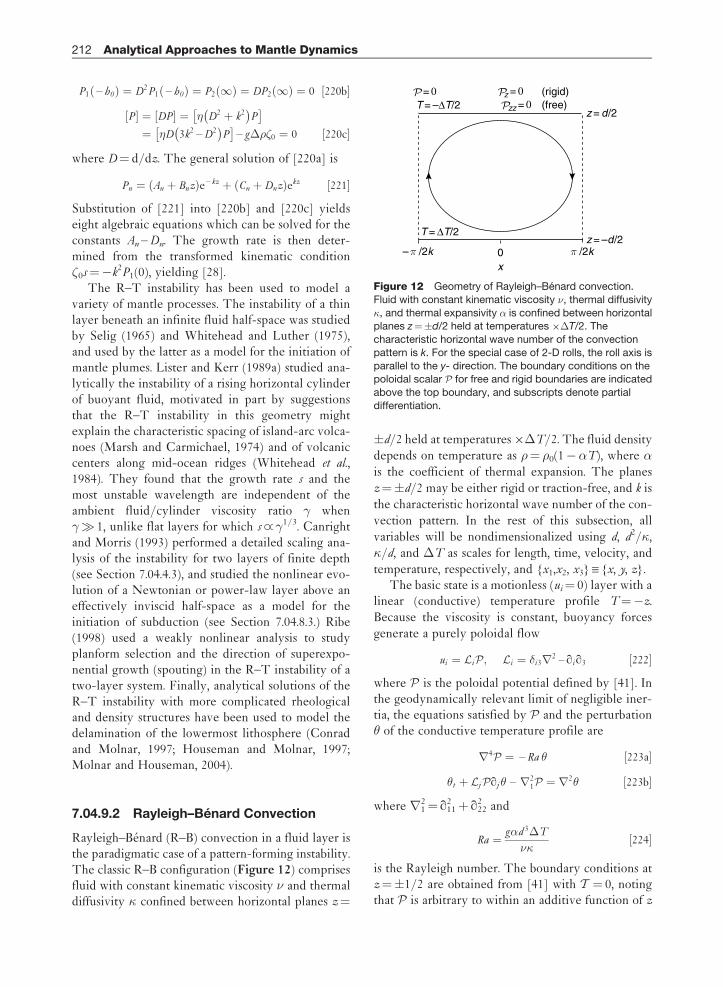
P1 – h0ð Þ ¼ D2P1 – h0ð Þ ¼ P2 1ð Þ ¼ DP2 1ð Þ ¼ 0 ½220b�

P½ � ¼ DP½ � ¼ � D2 þ k2� �

P

¼ �D 3k2 –D2� �

P

– g��0 ¼ 0 ½220c�

where D¼ d/dz. The general solution of [220a] is

Pn ¼ An þ Bnzð Þe – kz þ Cn þ Dnzð Þekz ½221�

Substitution of [221] into [220b] and [220c] yieldseight algebraic equations which can be solved for theconstants An – Dn. The growth rate is then deter-mined from the transformed kinematic condition0s¼�k2P1(0), yielding [28].

The R–T instability has been used to model avariety of mantle processes. The instability of a thinlayer beneath an infinite fluid half-space was studiedby Selig (1965) and Whitehead and Luther (1975),and used by the latter as a model for the initiation ofmantle plumes. Lister and Kerr (1989a) studied ana-lytically the instability of a rising horizontal cylinderof buoyant fluid, motivated in part by suggestionsthat the R–T instability in this geometry mightexplain the characteristic spacing of island-arc volca-noes (Marsh and Carmichael, 1974) and of volcaniccenters along mid-ocean ridges (Whitehead et al.,1984). They found that the growth rate s and themost unstable wavelength are independent of theambient fluid/cylinder viscosity ratio � when�� 1, unlike flat layers for which s _ �1/3. Canrightand Morris (1993) performed a detailed scaling ana-lysis of the instability for two layers of finite depth(see Section 7.04.4.3), and studied the nonlinear evo-lution of a Newtonian or power-law layer above aneffectively inviscid half-space as a model for theinitiation of subduction (see Section 7.04.8.3.) Ribe(1998) used a weakly nonlinear analysis to studyplanform selection and the direction of superexpo-nential growth (spouting) in the R–T instability of atwo-layer system. Finally, analytical solutions of theR–T instability with more complicated rheologicaland density structures have been used to model thedelamination of the lowermost lithosphere (Conradand Molnar, 1997; Houseman and Molnar, 1997;Molnar and Houseman, 2004).

7.04.9.2 Rayleigh–Benard Convection

Rayleigh–Benard (R–B) convection in a fluid layer isthe paradigmatic case of a pattern-forming instability.The classic R–B configuration (Figure 12) comprisesfluid with constant kinematic viscosity � and thermaldiffusivity � confined between horizontal planes z¼

d/2 held at temperatures��T/2. The fluid density

depends on temperature as �¼ �0(1�T), where is the coefficient of thermal expansion. The planes

z¼d/2 may be either rigid or traction-free, and k is

the characteristic horizontal wave number of the con-

vection pattern. In the rest of this subsection, all

variables will be nondimensionalized using d, d2/�,

�/d, and �T as scales for length, time, velocity, and

temperature, respectively, and {x1,x2, x3} X {x, y, z}.The basic state is a motionless (ui¼ 0) layer with a

linear (conductive) temperature profile T¼�z.

Because the viscosity is constant, buoyancy forces

generate a purely poloidal flow

ui ¼ L i P ; L i ¼ �i3r2 – qiq3 ½222�

where P is the poloidal potential defined by [41]. Inthe geodynamically relevant limit of negligible iner-tia, the equations satisfied by P and the perturbation� of the conductive temperature profile are

r4P ¼ –Ra � ½223a�

�t þ L j P qj � – r21P ¼ r2� ½223b�

where r12¼ q11

2 þ q222 and

Ra ¼ gd 3�T

��½224�

is the Rayleigh number. The boundary conditions atz¼1/2 are obtained from [41] with T ¼ 0, notingthat P is arbitrary to within an additive function of z

(rigid)(free)

T = ΔT/2

T = –ΔT/2 z = 0

π /2k– π /2k

z = d /2

z = –d /2

x0

= 0 zz = 0

Figure 12 Geometry of Rayleigh–Benard convection.

Fluid with constant kinematic viscosity �, thermal diffusivity

�, and thermal expansivity is confined between horizontalplanes z¼d/2 held at temperatures ��T/2. The

characteristic horizontal wave number of the convection

pattern is k. For the special case of 2-D rolls, the roll axis is

parallel to the y- direction. The boundary conditions on thepoloidal scalar P for free and rigid boundaries are indicated

above the top boundary, and subscripts denote partial

differentiation.


and/or an additive function f (x, y) satisfying r12f¼ 0.

Impermeability requires r12P ¼ 0, which can be

replaced by the simpler condition P ¼ 0. The no-slip condition at a rigid surface requires q13

2 P ¼ q232 P

¼ 0, which can be replaced by q3P ¼ 0. Finally, thevanishing of the tangential stress at a free surfacerequires q1 r2

1 – q233

� �P ¼ q2 r2

1 – q233

� �P ¼ 0, which

can be replaced by q332 P ¼ 0. In summary, the bound-

ary conditions are

� ¼ P ¼ q233P ¼ 0 freeð Þ ½225a�

or

� ¼ P ¼ q3P ¼ 0 rigidð Þ ½225b�

7.04.9.2.1 Linear stability analysis

The initial/BVP describing the evolution of smallperturbations to the basic state is obtained by linear-izing [223] about (P , �)¼ (0, 0), reducing theresulting equations to a single equation for P bycross-differentiation, and recasting the boundaryconditions �(1/2)¼ 0 in terms of P with the helpof [223a]. For the (analytically simpler) free-bound-ary case, the result is

r4 r2 – qt

� �–Rar2

1

P ¼ 0 ½226a�

P ¼ q233P ¼ q4

3333P ¼ 0 at z ¼ 1=2 ½226b�

Equations [226] admit normal mode solutions of theform

P ¼ P zð Þf x; yð Þest ½227�

where � is the growth rate and f (x,y) is the planformfunction satisfying r1

2f¼�k2f. Substituting [227]into [226], we obtain

D2 – k2� �2

D2 – k2 – s� �

þ Rak2h i

P ¼ 0 ½228a�

P ¼ D2P ¼ D4P ¼ 0 at z ¼ 1=2 ½228b�

where D¼ d/dz. Equations [228] define an eigenva-lue problem whose solution is

P ¼ sin n� zþ 1

2

� �; s ¼ Ra k2

n2�2 þ k2ð Þ2–n2�2 – k2 ½229�

where the index n defines the vertical wavelength ofthe mode. The growth rate s becomes positive when Ra

exceeds a value Ra0(k) that corresponds to marginalstability. This occurs first for the mode n¼ 1, for which

Ra0 ¼�2 þ k2ð Þ3

k2½230�

The most unstable wave number kc and the corre-sponding critical Rayleigh number Rac are found byminimizing Ra0(k), yielding

Rac ¼27�4

4 657:5; kc ¼

�ffiffiffi2p 2:22 ½231�

The corresponding results for convection between rigidsurfaces must be obtained numerically (Chandrasekhar,1981, pp. 36–42), and are Rac 1707.8, kc 3.117. Themarginally stable Rayleigh number Ra0(k) is shown forboth free and rigid surfaces in Figure 13(a). For futurereference, we note that [229] can be written

s ¼ �2 þ k2� � Ra – Ra0

Ra0½232�

7.04.9.2.2 Order-parameter equations for

finite-amplitude thermal convectionLinear stability analysis predicts the initial growthrate of a normal mode with wave number k.Typically, however, many different modes have thesame or nearly the same growth rate: examplesinclude convection rolls with the same wave numberbut different orientations, and rolls with the sameorientation but slightly different wave numberswithin a narrow band around the most unstablewave number kc. The question therefore arises:among a set of modes with equal (or nearly equal)growth rates, which mode or combination of modes isactually realized for a given (supercritical) Rayleighnumber? The answer depends on a combination oftwo factors: the nonlinear coupling between differentmodes due to the nonlinear terms in the governingequations, and external biases imposed by the initialand/or boundary conditions. Linear stability analysisis powerless to help us here, and more complicatednonlinear theories are required.

An especially powerful method of this type is toreduce the full 3-D equations governing convection to2-D equations for one or more order parameters thatdescribe the degree of order or patterning in thesystem. Newell et al. (1993) identified four distinctclasses of such equations, depending on whether thedegree of supercriticality X [(Ra� Rac)/Rac]

1/2 issmall or of order unity, and whether the horizontalspectrum of the allowable modes is discrete or (quasi-)continuous (Table 4). The spectrum is discrete forconvection in an infinite layer with a periodic plan-form characterized by a single fundamental wavenumber k, and also for a layer of finite extentL¼O (d ) when only a few of the allowable wave


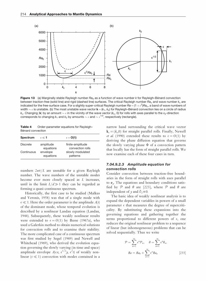
numbers 2n�/L are unstable for a given Rayleighnumber. The wave numbers of the unstable modesbecome ever more closely spaced as L increases,until in the limit L/d� 1 they can be regarded asforming a quasi-continuous spectrum.

Historically, the first case to be studied (Malkusand Veronis, 1958) was that of a single mode with � 1. Here the order parameter is the amplitude A(t)of the dominant mode, whose temporal evolution isdescribed by a nonlinear Landau equation (Landau,1944). Subsequently, these weakly nonlinear resultswere extended to ¼O (1) by Busse (1967a), whoused a Galerkin method to obtain numerical solutionsfor convection rolls and to examine their stability.The more complicated case of a continuous spectrumwas first studied by Segel (1969) and Newell andWhitehead (1969), who derived the evolution equa-tion governing the slowly varying (in time and space)amplitude envelope A( x, 1/2y, 2t) of weakly non-linear ( � 1) convection with modes contained in a

narrow band surrounding the critical wave vectorkc¼ (kc,0) for straight parallel rolls. Finally, Newellet al. (1990) extended these results to ¼O (1) byderiving the phase diffusion equation that governsthe slowly varying phase � of a convection patternthat locally has the form of straight parallel rolls. Wenow examine each of these four cases in turn.

7.04.9.2.3 Amplitude equation for

convection rolls

Consider convection between traction-free bound-aries in the form of straight rolls with axes parallelto ey. The equations and boundary conditions satis-fied by P and � are [223], where P and � areindependent of y and q2 X 0.

The basic idea of weakly nonlinear analysis is toexpand the dependent variables in powers of a smallparameter that measures the degree of supercriti-cality. By substituting these expansions into thegoverning equations and gathering together theterms proportional to different powers of , onereduces the original nonlinear problem to a sequenceof linear (but inhomogeneous) problems that can besolved sequentially. Thus we write

P ¼X1n¼1

nP n; � ¼X1n¼1

n�n;

Ra ¼ Ra0 þX1n¼1

nRan ½233�

Table 4 Order-parameter equations for Rayleigh–

Benard convection

Spectrum �1 ¼O(1)

Discrete amplitude

equations

finite-amplitude

convection rolls

Continuous envelope

equations

slowly modulated

patterns

0

1000

2000

4000

5000

6000

0 4 6 8

(a) (b)

Ra0

kc

k

Rac

kc

k1

k2

2Rac Ra

1/2∋

∋

∋

∋

Figure 13 (a) Marginally stable Rayleigh number Ra0 as a function of wave number k for Rayleigh–Benard convection

between traction-free (solid line) and rigid (dashed line) surfaces. The critical Rayleigh number Rac and wave number kc are

indicated for the free-surface case. For a slightly super-critical Rayleigh number Ra¼ (1þ 2)Rac, a band of wave numbers ofwidth � is unstable. (b) The most unstable wave vector k¼ (k1, k2) for Rayleigh–Benard convection lies on a circle of radius

kc. Changing jkj by an amount � in the vicinity of the wave vector (kc, 0) for rolls with axes parallel to the x2-direction

corresponds to changing k1 and k2 by amounts � and � 1/2, respectively (rectangle).


where the last expansion can be regarded as animplicit definition of the supercriticality (Ra). Nowbecause the boundary conditions are the same onboth surfaces, the hot and cold portions of the floware mirror images of each other. The problem istherefore invariant under the transformation {P !�P , �!��} or (equivalently) !� . Applicationof the latter transformation to the expanded form of[223a] shows that Ran¼ 0 for all odd n. To lowestorder, therefore,

Ra –Ra0 2Ra2 ½234�

where Ra2¼O (1) is to be determined. Now compar-ison of [234] with [232] shows that s _ 2. Wetherefore introduce a slow time T X 2t which is oforder unity during the initial stage of exponentialgrowth, whence

qt ¼ 2qT ½235�

Substituting [233], [234], and [235] into [223] andcollecting terms proportional to , we obtain

r4P 1 þ Ra0�1 ¼ 0; r2�1 þ q211P 1 ¼ 0 ½236�

subject to the boundary conditions P 1¼ q332 P 1¼ �1

¼ 0 at z¼1/2. This is just the linear stability pro-blem, for which the solution is

P 1 ¼ –C

k2cos�z cos kx; �1 ¼

C

�2 þ k2cos �z cos kx;

Ra0 ¼�2 þ k2ð Þ3

k2½237�

where the amplitude C(T) of the vertical velocityw1 X q11

2 P 1 remains to be determined. Next, we col-lect terms proportional to 2 to obtain

r4P 2 þ Ra0�2 ¼ –Ra1�1 X 0 ½238a�

r2�2 þ q211P 2 ¼ L j P 1qj �1 X –

C2�

2 �2 þ k2ð Þ sin 2�z ½238b�

Now because the inhomogeneous term in [238b]depends only on z, we must seek solutions of [238]of the forms

P 2 ¼ P 2 x; zð Þ; �2 ¼ �2 x; zð Þ þ ��2 zð Þ ½239�

where P~2 and �2 are the fluctuating (periodic in x)parts of the solution and ��2 is the mean (x-indepen-dent) part. The mean part of P 2 is set to zero becausethe poloidal scalar is arbitrary to within an additivefunction of z, as can be verified by inspection of [41].Now the equations satisfied by P~2 and �2 are just thehomogeneous forms of [238], which are identical tothe order equations [236]. We may therefore set

P~2¼ �2¼ 0 with no loss of generality. The solutionfor ��2 is then obtained by integrating [238b] subjectto the boundary conditions ��2(1/2)¼ 0. Wethereby find

P 2 ¼ 0; �2 X��2 ¼

C2

8� �2 þ k2ð Þ sin 2�z ½240�

Physically, ��2(z) describes the average heating (cool-ing) of the upper (lower) half of the layer that isinduced by the convection. Despite appearances,[240] is consistent with [238a] because P 2 is arbitraryto within an additive function of z.

The parameter Ra2 is still not determined, so wemust proceed to order 3, for which the equations are

r4P 3 þ Ra0�3 ¼ – Ra2�1 ½241a�

r2�3 þ q211P 3 ¼ qT�1 þ L j P 1qj �2 ½241b�

We now evaluate the RHSs of [241], set P 3¼ P~3(z,T )coskx and �3¼ �~3(z, T ) coskx, and reduce the resul-ting equations to a single equation for P~3, obtaining

D2 – k2� �3þk2Ra0

h iP~3

¼ –Ra0 C3 cos 2�zþ 4 _C� �

4 �2 þ k2ð Þ – Ra2C

" #cos �z ½242�

where D¼ d/dz and a superposed dot denotes d/dT.Now the homogeneous form of [242] is identical tothe eigenvalue problem at order , and thus has asolution _ cos �z that satisfies the boundary condi-tions. The Fredholm alternative theorem thenimplies that the inhomogeneous equation [242] willhave a solution only if the RHS satisfies a solvabilitycondition. In the general case, this condition is foundby multiplying the inhomogeneous equation by thesolution of the homogeneous adjoint problem andthen integrating over the domain of the dependentvariable. For our (self-adjoint) problem, the homo-geneous adjoint solution is _ cos �z, and theprocedure just described yieldsZ 1=2

– 1=2

��D2 – k2

�3

þ k2Ra0

�P 3 cos �z dz

¼ –

Ra0

�C3 þ 8 _C

�– 8��2 þ k2

�Ra2C

16��2 þ k2

� ½243�

Now the LHS of [243] is identically zero, as one caneasily show by integrating repeatedly by partsand applying the boundary conditions on P~3. TheRHS of [243] must therefore vanish. Now by [233]and [237], the amplitude of the vertical velocity is C XW. Because only the product of and C is phy-sically meaningful, the definition of itself – or,


equivalently, of Ra2 – is arbitrary. Making the mostconvenient choice Ra2¼ Ra0, we find that the vanish-ing of the RHS of [243] yields the followingevolution equation for the physical amplitude W:

dW

dT¼ �2 þ k2� �

W –Ra0

8 Ra –Ra0ð ÞW 3 ½244�

Initially, W grows exponentially with a growth rateW�1 _W ¼ �2þ k2. At long times, however, _W ! 0 andthe amplitude approaches a steady value

W T !1ð Þ ¼ 8 �2 þ k2ð Þ Ra – Ra0ð ÞRa0

� �1=2

½245�

7.04.9.2.4 Finite-amplitude convection

rolls and their stability

The extension of the above results to strongly non-linear rolls ( ¼O (1)) between rigid surfaces is due toBusse (1967a), whose development we follow herewith some changes of notation. The first step is todetermine steady roll solutions of [223] using aGalerkin method (Fletcher, 1984) whereby � and Pare expanded in orthogonal functions that satisfy theboundary conditions and the coefficients are thenchosen to satisfy approximately the governingequations.

We begin by expanding � into a complete set ofFourier modes that satisfy the boundary conditions�(x, 1/2)¼ 0:

� ¼Xm;n

cmneimkx fn zð Þ; fn zð Þ ¼ sin n� zþ 1

2

� �½246�

where 2�/k is the wavelength of the convection rolls,cmn¼ �cn�m, where the overbar denotes complex con-jugation, and the summations are over �1�m�1and 1� n�1. Now substitute [246] into [223a] andsolve the resulting equation to obtain

P ¼ –RaXm;n

cmneimkxQn mk; zð Þ ½247a�

Qn r ; zð Þ ¼ fn zð Þ þ n�hn rð Þr 2 þ n2�2ð Þ2

½247b�

hn rð Þ ¼2SC þ rð Þ – 1 2zC sin h rz – Scosh rzð Þ n oddð Þ

2SC – rð Þ – 1C sin h rz – 2zScosh rzð Þ n evenð Þ

(

½247c�

S ¼ sinhr

2; C ¼ cosh

r

2½247d�

To determine the coefficients cmn, we substitute [247]into [223b], multiply the result by fq(z)e�ipkx, andintegrate over the fluid layer. By using for p and q

all integers in the ranges of m and n, respectively, weobtain an infinite set of nonlinear algebraic equationsfor cmn(Ra) that can be truncated and solved numeri-cally (Busse, 1967a.)

Another advantage of the Galerkin method is thata stability analysis of the solution can easily be per-formed. The linearized equations governinginfinitesimal perturbations (P~, �) to the steady rollsolution (P 0, �0) are

r4P~¼ –Ra� ½248a�

�t þ L j P 0qj � þ qj �0L j P~–r21P~¼ r2� ½248b�

subject to �¼ P~¼ q3P~¼ 0 at z¼1/2. Now [248]are linear PDEs with coefficients that are periodic inthe x-direction but independent of both z and t. Thegeneral solution can be written as a sum of solutionswhich depend exponentially on x, y, and t, multipliedby a function of x having the same periodicity as thestationary solution (Busse, 1967a.) We therefore write

� ¼Xm;n

cmneimkxfn zð Þ( )

ei axþbyð Þþst ½249�

and note further that [248a] and the boundary con-ditions on P

˜are satisfied exactly if

P~¼ –RaXm; n

cmneimkxQn

ffiffiffiffiffiffiffiffiffiffiffiffiffiffiffiffiffiffiffiffiffiffiffiffiffiffiffimk þ að Þ2þb2

q; z

� �( )

� ei axþbyð Þþst ½250�

Substituting [249] and [250] into [248b], multiplyingby fq(z)e�i(pkxþ axþ by)�st, and averaging over the fluidlayer, we obtain an infinite system of linear equationsfor the coefficients cmn. The system is then truncatedand the largest eigenvalue s(Ra, k, a, b) is determinednumerically, assuming that s is real in view of the factthat I(s)¼ 0 at the onset of convection (Busse,1967a).

The results show that convection rolls are stable(s < 0) in an elongate region of the (Ra, k) space oftencalled the Busse balloon (Figure 14). AboveRa 22600, convection rolls of any wave numberare unstable. The lower left edge of the balloon(denoted by Z in Figure 14) represents the onset ofa zigzag instability in the form of rolls oblique to theoriginal ones. Around the rest of the balloon (denotedby C), the stability of rolls is limited by the crossrollinstability, which grows in the form of perpendicu-larly aligned rolls. The results of Busse (1967a) wereextended to the case of traction-free boundaries byStraus (1972), Busse and Bolton (1984), and Boltonand Busse (1985).


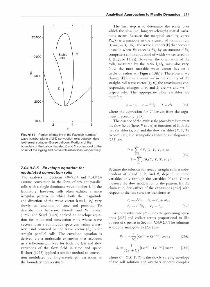
7.04.9.2.5 Envelope equation for

modulated convection rolls

The analyses in Sections 7.04.9.2.3 and 7.04.9.2.4

assume convection in the form of straight parallel

rolls with a single dominant wave number k. In the

laboratory, however, rolls often exhibit a more

irregular pattern in which both the magnitude

and direction of the wave vector k¼ (k1, k2) vary

slowly as functions of time and position. To

describe this behavior, Newell and Whitehead

(1969) and Segel (1969) derived an envelope equa-

tion for modulated convection rolls whose wave

vectors form a continuous spectrum within a nar-

row band centered on the wave vector (kc, 0) for

straight parallel rolls. The envelope equation is

derived via a multiscale expansion that accounts

in a self-consistent way for both the fast and slow

variations of the flow field in time and space.

Richter (1973) applied a similar method to convec-

tion modulated by long-wavelength variations in

the boundary temperatures.

The first step is to determine the scales overwhich the slow (i.e., long-wavelength) spatial varia-

tions occur. Because the marginal stability curve

Ra0(k) is a parabola in the vicinity of its minimum

(k, Ra0)¼ (kc, Rac), the wave numbers jkj that become

unstable when Ra exceeds Rac by an amount 2Rac

comprise a continuous band of width � centered on

kc (Figure 13(a)). However, the orientation of the

rolls, measured by the ratio k2/k1, may also vary.

Now the most unstable wave vector lies on a

circle of radius kc (Figure 13(b)). Therefore if we

change jkj by an amount � in the vicinity of the

straight-roll wave vector (kc, 0), the (maximum) cor-

responding changes of k1 and k2 are � and � 1/2,

respectively. The appropriate slow variables are

therefore

X ¼ x; Y ¼ 1=2y; T ¼ 2t ½251�

where the expression for T derives from the argu-ment preceeding [235].

The essence of the multiscale procedure is to treatthe flow fields (here, P and �) as functions of both the

fast variables (x, y, t) and the slow variables (X, Y, T).

Accordingly, the asympotic expansions analogous to

[233] are

P ¼X1n¼1

nP n X ; Y ; T ; x; zð Þ

� ¼X1n¼1

n�n X ; Y ; T ; x; zð Þ½252�

Because the solution for steady straight rolls is inde-pendent of y and t, P n and �n depend on thesevariables only through the variables Y and T thatmeasure the slow modulation of the pattern. By thechain rule, derivatives of the expansions [252] withrespect to the fast variables transform as

qt ! 2qT ; qx ! qx þ qX ;

qy ! 1=2qY ; qz ! qz ½253�

We now substitute [252] into the governing equa-tions [223] and collect terms proportional to like

powers of , just as in Section 7.04.9.2.3. The solutions

at order analogous to [237] are

P 1 ¼ –1

2k2c

Ceikcx þ �Ce – ikcx

cos �z ½254a�

�1 ¼1

2 �2 þ k2c

� � Ceikcx þ �Ce – ikcx

cos�z ½254b�

where C¼C(X, Y, T) is the slowly varying envelopeof the roll solution and overbars denotes complex

1000

2000

5000

10 000

20 000

2 4 6

Z

CStable rolls

Ra

k

Figure 14 Region of stability in the Rayleigh number/

wave number plane of 2-D convection rolls between rigidisothermal surfaces (Busse balloon). Portions of the

boundary of the balloon labeled Z and C correspond to the

onset of the zigzag and cross-roll instabilities, respectively.


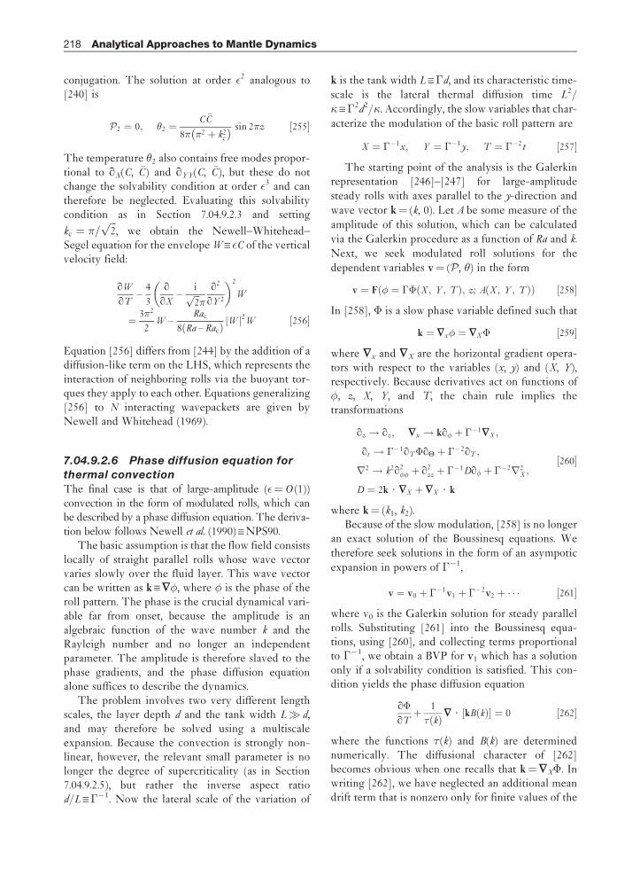
conjugation. The solution at order 2 analogous to[240] is

P 2 ¼ 0; �2 ¼C �C

8� �2 þ k2c

� � sin 2�z ½255�

The temperature �2 also contains free modes propor-tional to qX(C, �C) and qYY(C, �C), but these do notchange the solvability condition at order 3 and cantherefore be neglected. Evaluating this solvabilitycondition as in Section 7.04.9.2.3 and setting

kc ¼ �=ffiffiffi2p

, we obtain the Newell–Whitehead–Segel equation for the envelope W X C of the verticalvelocity field:

qW

qT–

4

3

qqX

–iffiffiffi2p�

q2

qY 2

� �2

W

¼ 3�2

2W –

Rac

8 Ra – Racð Þ Wj j2W ½256�

Equation [256] differs from [244] by the addition of adiffusion-like term on the LHS, which represents theinteraction of neighboring rolls via the buoyant tor-ques they apply to each other. Equations generalizing[256] to N interacting wavepackets are given byNewell and Whitehead (1969).

7.04.9.2.6 Phase diffusion equation for

thermal convection

The final case is that of large-amplitude ( ¼O (1))convection in the form of modulated rolls, which canbe described by a phase diffusion equation. The deriva-tion below follows Newell et al. (1990)XNPS90.

The basic assumption is that the flow field consistslocally of straight parallel rolls whose wave vectorvaries slowly over the fluid layer. This wave vectorcan be written as k X��, where � is the phase of theroll pattern. The phase is the crucial dynamical vari-able far from onset, because the amplitude is analgebraic function of the wave number k and theRayleigh number and no longer an independentparameter. The amplitude is therefore slaved to thephase gradients, and the phase diffusion equationalone suffices to describe the dynamics.

The problem involves two very different lengthscales, the layer depth d and the tank width L� d,and may therefore be solved using a multiscaleexpansion. Because the convection is strongly non-linear, however, the relevant small parameter is nolonger the degree of supercriticality (as in Section7.04.9.2.5), but rather the inverse aspect ratiod/L X��1. Now the lateral scale of the variation of

k is the tank width L X�d, and its characteristic time-

scale is the lateral thermal diffusion time L2/

� X�2d2/�. Accordingly, the slow variables that char-

acterize the modulation of the basic roll pattern are

X ¼ � – 1x; Y ¼ � – 1y; T ¼ � – 2t ½257�

The starting point of the analysis is the Galerkinrepresentation [246]–[247] for large-amplitude

steady rolls with axes parallel to the y-direction and

wave vector k¼ (k, 0). Let A be some measure of the

amplitude of this solution, which can be calculated

via the Galerkin procedure as a function of Ra and k.

Next, we seek modulated roll solutions for the

dependent variables v¼ (P , �) in the form

v ¼ F � ¼ �� X ; Y ; Tð Þ; z; A X ; Y ; Tð Þð Þ ½258�

In [258], � is a slow phase variable defined such that

k ¼ �x� ¼ �X � ½259�

where �x and �X are the horizontal gradient opera-tors with respect to the variables (x, y) and (X, Y),respectively. Because derivatives act on functions of�, z, X, Y, and T, the chain rule implies thetransformations

qz ! qz; �x ! kq� þ � – 1�X ;

qt ! � – 1qT �qY þ � – 2qT ;

r2 ! k2q2�� þ q2

zz þ � – 1Dq� þ � – 2r2X ;

D ¼ 2k ? �X þ �X ? k

½260�

where k¼ (k1, k2).Because of the slow modulation, [258] is no longer

an exact solution of the Boussinesq equations. We

therefore seek solutions in the form of an asympotic

expansion in powers of ��1,

v ¼ v0 þ � – 1v1 þ � – 2v2 þ � � � ½261�

where v0 is the Galerkin solution for steady parallelrolls. Substituting [261] into the Boussinesq equa-tions, using [260], and collecting terms proportionalto ��1, we obtain a BVP for v1 which has a solutiononly if a solvability condition is satisfied. This con-dition yields the phase diffusion equation

q�

qTþ 1

� kð Þ� ? kB kð Þ½ � ¼ 0 ½262�

where the functions � (k) and B(k) are determinednumerically. The diffusional character of [262]becomes obvious when one recalls that k¼�X�. Inwriting [262], we have neglected an additional meandrift term that is nonzero only for finite values of the


Prandtl number (NPS90, eqn. (1.1)). NPS90 showthat a linear stability analysis of [262] reproducesclosely all the portions of the boundary of the Busseballoon for which the wavelength of the instability islong relative to the layer depth.

7.04.9.3 Convection at High RayleighNumber

Even though convection in the form of steady 2-Drolls is unstable when Ra > 22 600 (Section 7.04.9.2.4),much can be learned by studying the structure ofsuch rolls in the limit Ra!1. Because temperaturevariations are now confined to thin TBLs around theedges of the cells, scaling analysis and BL theory areparticularly effective tools for this purpose.

7.04.9.3.1 Scaling analysis

The essential scalings for cellular convection at highRayleigh number can be determined by a scalinganalysis of the governing equations. The followingderivation (for the cell geometry shown in Figure 6)generalizes the analysis of McKenzie et al. (1974) toinclude both traction-free and rigid-surface bound-ary conditions. For simplicity, we assume in thissubsection only that the aspect ratio � does not differmuch from unity.

The analysis proceeds by determining six equa-tions relating six unknown quantities: the thicknesses�p of the thermal plumes and �h of the horizontalTBLs, the maximum vertical velocity vp and thevorticity ! in the plumes, the vertical velocity v(�h)in the plume at the edge of the horizontal BLs, andthe heat flux q across the layer (per unit length alongthe roll axes). The heat flux carried by an upwellingplume is

q � �cpvp�T�p ½263�

where cp is the heat capacity at constant pressure.Because the convection is steady, the flux [263]must equal that lost by conduction through the tophorizontal BL, implying

q � kcd�T=�h ½264�

where kc is the thermal conductivity. The thickness�h of the horizontal BLs is controlled by the balancevTy��Tyy of advection and diffusion, which implies

v �hð Þ�T=�h � ��T=�2h ½265�

Now u(�h) depends on whether the horizontal sur-faces are free or rigid. Because the velocity parallel to

the boundary is constant to lowest order across aTBL at a free surface (n¼ 0 say) and varies linearlyacross a TBL at a rigid surface (n¼ 1),

v �hð Þ � vp �h=dð Þnþ1 ½266�

The force balance in the plumes is scaled using thevorticity equation �r2!¼ gTx, which implies

! � g�T�p=� ½267�

Finally, the vorticity ! in the plumes is of the sameorder as the rotation rate of the isothermal core, or

! � vp=d ½268�

The simultaneous solution of [263]–[268] yieldsscaling laws for each of the six unknown quantities asa function of R. Table 5 shows the results for vp, �p,and the Nusselt number Nu X d/�h. The free-surfaceheat transfer law Nu� Ra1/3 corresponds to a dimen-sional heat flux q X kc�TNu/d that is independent ofthe layer depth d, whereas q _ d�2/5 for rigid surfaces.A revealing check of the results is to note that vpd/�(column 2) is just the effective Peclet number Pe forthe flow. The scaling laws for Nu (column 4) thenimply Nu� Pe1/(nþ 2), in agreement with our pre-vious expression [12] for the heat transfer from ahot sphere moving in a viscous fluid.

7.04.9.3.2 Flow in the isothermal core

Given the fundamental scales of Table 5, we cannow carry out a more detailed analysis based on BLtheory. This approach, pioneered by Turcotte (1967)and Turcotte and Oxburgh (1967) and extended byRoberts (1979), Olson and Corcos (1980), andJimenez and Zufiria (1987) (henceforth JZ87), isapplicable to convection in a layer bounded by eitherfree or rigid surfaces. Here we consider only theformer case, following JZ87 with some changes ofnotation.

The dimensional equations governing the flow are

�r4 ¼ – gTx ½269a�

u�x þ v�y ¼ �r2T ½269b�

Table 5 Scaling laws for vigorous Rayleigh–Benard

convection

Boundaries vpd/� �p/d Nu Xd/�h

Free Ra2/3 Ra�1/3 Ra1/3

Rigid Ra3/5 Ra�2/5 Ra1/5


where T is the temperature, u¼ uexþ vey X� yexþ xey is the velocity, and is the streamfunction. Inthe limit Ra!1, each cell comprises a nearly iso-thermal core surrounded by thin vertical plumes andhorizontal BLs. Because temperature gradients arenegligible in the core, the principal agency drivingthe flow within it is the shear stresses applied to itsvertical boundaries by the plumes. Our first task istherefore to derive a boundary condition on the coreflow that represents this agency.

Consider for definiteness the upwelling plume at theleft boundary x¼��d/2 X x� of the cell (Figure 6),

and let its half-width be �p. The (upward) buoyancy

force acting on the right half of this plume must

be balanced by a downward shear stress at its edge

x¼ x�þ �p (the shear stress on x¼ x� is zero by

symmetry). This requires

�vx jx¼x –þ�p¼ – g

Z x –þ�p

x –

T –Tcð Þdx ½270�

where Tc (X 0) is the temperature in the core.Multiplying [270] by vp, we obtain

vpvx jx¼x –þ�p¼ –

g

��cp�cp

Z x –þ�p

x –

vp T –Tcð Þdx

� �½271�

where we have used the fact that vp X x is constant tofirst order across the plumes to take it inside theintegral on the RHS. Now the quantity [. . .] in[270] is just the heat flux carried by the right half ofthe plume, which is kc�TNu/2. Moreover, becausethe plume is thin, vx X xx can be evaluated at x¼ x�rather than at x¼ x�þ �p. Equation [271] thenbecomes

x xx jx¼x –¼ –

1

2

g��T

�Nu ½272�

which is a nonlinear and inhomogeneous boundarycondition on the core flow. The corresponding con-dition at x¼þ�d/2 is obtained from [272] byreversing the sign of the RHS.

We now invoke the results of the scaling analysis(Table 5) to nondimensionalize the equations and

boundary conditions for the core flow. We first write

the scaling law for Nu as

Nu ¼ C �ð ÞRa1=3 ½273�

where C(�) (to be determined) measures the depen-dence of the heat transfer on the aspect ratio.Rewriting the equations and boundary conditions interms of the dimensionless variables (x9, z9)¼ (x, z)/d

and 9¼ /�C(�)1/2Ra2/3 and then dropping theprimes, we obtain

r4 ¼ 0 ½274a�

x; 1=2ð Þ ¼ yy x; 1=2ð Þ ¼ 0 ½274b�

�=2; yð Þ ¼ x �=2; yð Þ� xx �=2; yð Þ�1=2 ¼ 0 ½274c�

The problem [274] can be solved either numerically(JZ87) or using a superposition method (Section7.04.5.4.1).

7.04.9.3.3 TBLs and heat transfer

The next step is to determine the temperature in theplumes and the horizontal TBLs using BL theory. Thetemperature in all these layers is governed by thetransformed BL equation [149]. Turcotte andOxburgh (1967) solved this equation assuming self-similarity, obtaining solutions of the form [151].However, Roberts (1979) pointed out that this is notcorrect, because the fluid traveling around the marginsof the cell sees a periodic boundary condition which isalternatingly isothermal (along the horizontal bound-aries) and insulating (in the plumes). Now because[149] is parabolic, its solution can be written in con-volution-integral form in terms of an arbitraryboundary temperature Tb(�) and an initial tempera-ture profile T( , 0) at � ¼ 0, where � ¼

RU(s)ds is the

time-like variable introduced in Section 7.04.7.1.1 andthe velocity U(s) parallel to the boundary is deter-mined (to within the unknown scale factor C(�))from the core flow streamfunction that satisfies[274]. However, in the limit �!1 correspondingto an infinite number of transits around the cell, theconvolution integral describing the evolution of theinitial profile vanishes, and the solution is (JZ87)

T ; �ð Þ ¼ –

2 ��ð Þ1=2

�Z 1

0

Tb � – tð Þt 3=2

exp – 2

4�t

� �dt ½275�

where all variables are dimensional. Now Tb isknown only on the top and bottom surfaces. Alongthe (insulating) plume centerlines, it can be found bysetting to zero the temperature gradient q T j ¼ 0

calculated from [275] and solving numerically theresulting integral equation. The temperature every-where in the plumes and horizontal BLs can then bedetermined from [275]. The final step is to determinethe unknown scale factor C(�) by matching the heatflow advected vertically by the plumes to the


conductive heat flux across the upper boundary(JZ87, eqn [23]).

The solution of JZ87 shows that the scale factorC(�) (and hence the Nusselt number Nu¼CRa1/3) ismaximum for � 0.75, which may therefore be thepreferred cell aspect ratio (Malkus and Veronis,1958). A particularly interesting result from a geo-physical perspective is that the temperature profile inthe TBL beneath the cold upper surface exhibits ahot asthenosphere, that is, a range of depths wherethe temperature exceeds that of the cell’s interior.

7.04.9.3.4 Structure of the flow near the

corners

The solutions described above break down near thecorners of the cell, where the vorticity of the coreflow solution becomes infinite and the BL approxi-mation is no longer valid. The (dimensional)characteristic radius rc of this corner region can bedetermined using a scaling argument. Consider fordefiniteness the corner above the upwelling plume,and let (r, ’) be polar coordinates with origin at thecorner such that ’¼ 0 on the upper surface and’¼ �/2 on the plume centerline. Close to the corner,the streamfunction has the self-similar form (r,’)¼ r�F(’) for some �, where F is given by [64].Near the corner, the dimensional forms of the bound-ary conditions [274b] and [274c] are

r ; 0ð Þ ¼ r ; �=2ð Þ ¼ ’’ r ; 0ð Þ ¼ 0 ½276a�

r – 3 ’ r ; �=2ð Þ ’’ r ; �=2ð Þ ¼ 1

2

g��T

�Nu ½276b�

Equation [276b] immediately implies �¼ 3/2, andthe streamfunction which satisfies all the conditions[276] is

¼ �2

r

d

� �3=2

C �ð Þ1=2Ra2=3 sin

3

2’ – sin

1

2’

� �½277�

Note that the vorticity !��(�/d2)Ra2/3(r/d)�1/2

becomes infinite at the corner. Now the balancebetween viscous forces and buoyancy in the cornerregion requires �r4 ��gTx, or

� �Ra rc=dð Þ3 ½278�

Equating [278] with the scale ��Ra2/3(rc/d)3/2

implied by [277], we find (Roberts, 1979)

rc � Ra – 2=9d ½279�

A corrected solution for the flow in the corner regionthat removes the vorticity singularity was proposedby JZ87.

7.04.9.3.5 Howard’s scaling for high-Ra

convection

While the above solution for cellular convection isilluminating, we know that rolls between rigidboundaries with R > 22 600 are not stable to smallperturbations (Section 7.04.9.2.4). In reality, convec-tion at high Rayleigh number Ra > 106 is a quasi-periodic process in which the TBLs grow by thermaldiffusion, become unstable, and then empty rapidlyinto plumes, at which point the cycle begins again.The characteristic timescale of this process can beestimated via a simple scaling argument (Howard,1964). The thickness � of both TBLs initiallyincreases by thermal diffusion as � (��t)1/2.Instability sets in when the growth rate of R–Tinstabilities in the layers (see Section 7.04.9.1)becomes comparable to the thickening rate _�/�,or (equivalently) when the Rayleigh numberRa(�) X g�T�3/�� based on the TBL thicknessattains a critical value Rac 103. This occurs after atime

tc 1

��

��Rac

g�T

� �2=3

½280�

that is independent of the layer depth. The scalinglaw [280] has been amply confirmed by laboratoryexperiments (e.g., Sparrow et al., 1970.)

7.04.9.4 Thermal Convection in MoreRealistic Systems

As the simplest and most widely studied example ofthermal convection, the R–B configuration is thesource of most of what has been learned aboutthermal convection during the past century. Froma geophysical point of view, however, it lacksmany crucial features that are important in theEarth’s mantle: the variation of viscosity as a functionof pressure, temperature, and stress; the presence ofsolid-state phase changes; internal production of heatby radioactive decay; density variations associatedwith differences in chemical composition; and ahost of other factors such as rheological anisotropy,the effect of volatile content, etc. Because analyticalmethods thrive on simple model problems, the addi-tion of each new complexity reduces their room formanoeuvre; but many important analytical resultshave been obtained nevertheless. Here we reviewbriefly some of these, focussing on the effects ofvariable viscosity, phase transitions, and chemicalheterogeneity.


A variety of important analytical results have beenobtained for fluids with temperature-dependent visc-osity. Stengel et al. (1982) performed a linear stabilityanalysis of convection in a fluid whose viscosity �(T)varies strongly (by up to a factor of 2� 104) withtemperature. For fluids for which �(T) is an expo-nential function, the critical Rayleigh number (basedon the viscosity at the mean of the boundary tem-peratures) first increases and then decreases as thetotal viscosity contrast across the layer increases,reflecting the fact that convection begins first in alow-viscosity sublayer near the hot bottom boundary.A nonlinear stability analysis of convection in a fluidwith a weak linear dependence of viscosity on tem-perature was carried out by Palm (1960), using amethod like that described in Section 7.04.9.2.3.Because the variation of the viscosity breaks thesymmetry between upwelling and downwellingmotions, the amplitude equation analogous to [244]contains a quadratic term that permits transcriticalbifurcation. Subsequent work (e.g., Busse, 1967b,Palm et al., 1967) showed that the stable planformsare hexagons, hexagons and 2D rolls, or 2D rollsalone, depending on the Rayleigh number. Busseand Frick (1985) used a Galerkin method (Section7.04.9.2.4) to study convection in a fluid whose visc-osity depends strongly (but linearly) on temperature,and found that a square planform becomes stablewhen the viscosity contrast is sufficiently large.

Convection at high Rayleigh number in fluidswith strongly variable viscosity is a particularly diffi-cult analytical challenge, but some noteworthyresults have been obtained. Morris and Canright(1984) and Fowler (1985) used BL analyses similarto that described in Section 7.04.9.3 to determinethe Nusselt number in the stagnant lid limit�T/�Tr!1 for convection in a fluid whoseviscosity depends on temperature as� ¼ �0exp – T –T0ð Þ=�Tr½ �. Both studies find theNusselt number to be Nu � �T=�Trð Þ – 1

Ra1=5r

where Ra�¼g�Trd3/�0� is the Rayleigh number

based on the rheological temperature scale �Tr andthe viscosity �0 at the hot bottom boundary.Solomatov (1995) presented a comprehensive scalinganalysis for convection in fluids with temperature-and stress-dependent viscosity. He found that threedifferent dynamical regimes occur as the total visc-osity contrast across the layer increases: quasi-isoviscous convection, a transitional regime with amobile cold upper BL, and a stagnant-lid regime inwhich the upper BL is motionless and convection isconfined beneath it. Busse et al. (2006) generalized

Turcotte and Oxburgh’s (1967) BL analysis of steadycellular convection to include thin low-viscositylayers adjoining the top and bottom boundaries,whose presence increases the cell aspect ratio thatmaximizes the heat transport.

The influence of a phase transition on the stabilityof convection in a fluid with constant viscosity wasanalyzed by Schubert and Turcotte (1971). Thenovel elements here are two matching conditions atthe depth of the phase change: one of these equatesthe energy released by the transformation to thedifference in the perturbation heat flux into and outof the phase boundary, while the second requires thephase boundary to lie on the Clapeyron slope. Theresulting eigenvalue problem yields the criticalRayleigh number Rac(S, RaQ), where

S ¼ ��=�

d �g=� –�ð Þ ; RaQ ¼gd 3Q

8cp��½281�

�� is the density difference between the phases, Q isthe energy per unit mass required to change thedenser phase into the lighter, � is the Clapeyronslope, and � is the magnitude of the temperaturegradient in the basic state. Rac is a decreasing functionof S (which measures the destabilizing effect of thedensity change) but an increasing function of RaQ

(which measures the stabilizing influence of latentheat). These results were extended to a divariantphase change by Schubert et al. (1972).

Convection in a chemically layered mantle wasfirst studied by Richter and Johnson (1974), whoperformed a linear stability analysis of a system com-prising two superposed fluid layers of equal depthand viscosity but different densities. The criticalRayleigh number Rac depends on the value of asecond Rayleigh number Ra�¼ g��d3/�� propor-tional to the magnitude of the stabilizing densitydifference �� between the layers. Three distinctmodes of instability are possible: convection overthe entire depth of the fluid with advection of theinterface; separate convection within each layer; andstanding waves on the interface, corresponding to animaginary growth rate at marginal stability. Busse(1981) extended these results to layers of differentthicknesses. Rasenat et al. (1989) examined a stilllarger region of the parameter space, and demon-strated the possibility of an oscillatory two-layerregime with no interface deformation, in which thecoupling between the layers oscillates between ther-mal and mechanical. Le Bars and Davaille (2002)mapped out the linear stability of two-layer


convection as a function of the interlayer viscositycontrast � and the layer depth ratio r, and showedthat the transition from oscillatory to stratified con-vection occurs at a critical value of the buoyancyratio B X Ra�/Ra that depends on � and r.

For the time being, studies like those discussedabove represent the limit of what can be learnedabout convection in complex systems using analyticalmethods alone. The impressive additional progressthat has been made using experimental and numer-ical approaches is discussed in Chapters 7.02 and 7.04of this volume.

Acknowledgment

This is IPGP contribution number 2202.

References

Albers M and Christensen UR (2001) Channeling of plume flowbeneath mid-ocean ridges. Earth and Planetary ScienceLetters 187: 207–220.

Ansari A and Morris S (1985) The effects of a stronglytemperature-dependent viscosity on Stokes’s drag law:Experiments and theory. Journal of Fluid Mechanics159: 459–476.

Backus GE (1958) A class of self-sustaining dissipativespherical dynamos. Annals of Physics 4: 372–447.

Bai Q, Mackwell SJ, and Kohlstedt DL (1991) High-temperaturecreep of olivine single crystals. Part 1: Mechanical results forbuffered samples. Journal of Geophysical Research96: 2441–2463.

Backus GE (1967) Converting vector and tensor equations toscalar equations in spherical co-ordinates. GeophysicalJournal of the Royal Astronomical Society 13: 71–101.

Barcilon V and Richter FM (1986) Nonlinear waves incompacting media. Journal of Fluid Mechanics164: 429–448.

Barenblatt GI (1996) Scaling, Self-Similarity, and IntermediateAsymptotics. Cambridge: Cambridge University Press.

Batchelor GK (1967) An Introduction to Fluid Dynamics.Cambridge: Cambridge University Press.

Batchelor GK (1970) Slender-body theory for particles ofarbitrary crosssection in Stokes flow. Journal of FluidMechanics 44: 419–440.

Bercovici D (1994) A theoretical model of cooling viscous gravitycurrents with temperature-dependent viscosity. GeophysicalResearch Letters 21: 1177–1180.

Bercovici D and Lin J (1996) A gravity current model of coolingmantle plume heads with temperature-dependent buoyancyand viscosity. Journal of Geophysical Research101: 3291–3309.

Biot MA (1954) Theory of stress-strain relations in anisotropicviscoelasticity and relaxation phenomena. Journal of AppliedPhysics 25: 1385–1391.

Bird RB, Armstrong RC, and Hassager O (1987) Dynamics ofPolymeric Liquids, Vol 1: Fluid Mechanics, 2nd edn. NewYork, NY: John Wiley & Sons.

Blake JR (1971) A note on the image system for a Stokeslet in ano-slip boundary. Proceedings of the CambridgePhilosophical Society 70: 303–310.

Bloor MIG and Wilson MJ (2006) An approximate analyticsolution method for the biharmonic problem. Proceedings ofthe Royal Society of London A 462: 1107–1121.

Bolton EW and Busse FH (1985) Stability of convection rolls in alayer with stress-free boundaries. Journal of Fluid Mechanics150: 487–498.

Buckingham E (1914) On physically similar systems; illustrationsof the use of dimensional equations. Physical Review4: 345–376.

Buckmaster JD, Nachman A, and Ting L (1975) The buckling andstretching of a viscida. Journal of Fluid Mechanics 69: 1–20.

Busse FH (1967a) On the stability of two-dimensionalconvection in a layer heated from below. Journal ofMathematical Physics 46: 140–150.

Busse FH (1967b) The stability of finite amplitude cellularconvection and its relation to an extremum principle. Journalof Fluid Mechanics 30: 625–649.

Busse FH (1981) On the aspect ratio of two-layer mantleconvection. Physics of the Earth and Planetary Interiors24: 320–324.

Busse FH and Bolton EW (1984) Instabilities of convection rollswith stress-free boundaries near threshold. Journal of FluidMechanics 146: 115–125.

Busse FH and Frick H (1985) Square-pattern convection influids with strongly temperature-dependent viscosity.Journal of Fluid Mechanics 150: 451–465.

Busse FH, Richards MA, and Lenardic A (2006) A simple modelof high Prandtl and high Rayleigh number convectionbounded by thin low-viscosity layers. Geophysical JournalInternational 164: 160–167.

Canright DR (1987) A Finite-Amplitude Analysis of the BuoyantInstability of a Highly Viscous Film over a Less Viscous Half-Space. PhD Thesis, University of California, Berkeley.

Canright D and Morris S (1993) Buoyant instability of a viscousfilm over a passive fluid. Journal of Fluid Mechanics255: 349–372.

Chandrasekhar S (1981) Hydrodynamic and HydromagneticStability. New York, NY: Dover.

Conrad CP and Molnar P (1997) The growth of Rayleigh–Taylor-type instabilities in the lithosphere for variousrheological and density structures. Geophysical JournalInternational 129: 95–112.

Cox RG (1970) The motion of long slender bodies in a viscousfluid. Part 1: General theory. Journal of Fluid Mechanics44: 791–810.

Davaille A (1999) Two-layer thermal convection in miscibleviscous fluids. Journal of Fluid Mechanics 379: 223–253.

Dziewonski AM and Anderson DL (1981) Preliminary referenceEarth model. Physics of the Earth and Planetary Interiors25: 297–356.

England P and McKenzie D (1983) Correction to: A thin viscoussheet model for continental deformation. GeophysicalJournal of the Royal Astronomical Society 73: 523–532.

Farrell WE (1972) Deformation of the Earth by surface loads.Review of Geophysics and Space Physics 10: 761–797.

Feighner M and Richards MA (1995) The fluid dynamics ofplume-ridge and plume-plate interactions: An experimentalinvestigation. Earth and Planetary Science Letters129: 171–182.

Fenner RT (1975) On local solutions to non-Newtonian slowviscous flows. International Journal of Non-Linear Mechanics10: 207–214.

Fleitout L and Froidevaux C (1983) Tectonic stresses in thelithosphere. Tectonics 2: 315–324.

Fletcher CAJ (1984) Computational Galerkin Methods. NewYork, NY: Springer Verlag.


Forte AM and Peltier WR (1987) Plate tectonics and asphericalEarth structure: The importance of poloidal-toroidalcoupling. Journal of Geophysical Research 92: 3645–3679.

Fowler AC (1985) Fast thermoviscous convection. Studies inApplied Mathematics 72: 189–219.

Gantmacher FR (1960) Matrix Theory, 2 vols. Providence, RI:AMS Chelsea Publishing.

Gomilko AM, Malyuga VS, and Meleshko VV (2003) On steadyStokes flow in a trihedral rectangular corner. Journal of FluidMechanics 476: 159–177.

Gratton J and Minotti F (1990) Self-similar viscous gravitycurrents: Phase-plane formalism. Journal of Fluid Mechanics210: 155–182.

Griffiths RW (1986) Thermals in extremely viscous fluids,including the effects of temperature-dependent viscosity.Journal of Fluid Mechanics 166: 115–138.

Hager BH and O’Connell RJ (1981) A simple global model ofplate tectonics and mantle convection. Journal ofGeophysical Research 86: 4843–4867.

Hager BH, Clayton RW, Richards MA, Comer RP, andDziewonski AM (1985) Lower mantle heterogeneity, dynamictopography and the geoid. Nature 313: 541–545.

Happel J and Brenner H (1991) Low Reynolds NumberHydrodynamics, 2nd rev. edn. Dordrecht: Kluwer Academic.

Hauri EH, Whitehead JA, Jr., and Hart SR (1994) Fluid dynamicand geochemical aspects of entrainment in mantle plumes.Journal of Geophysical Research 99: 24275–24300.

Hinch EJ (1991) Perturbation Methods. Cambridge: CambridgeUniversity Press.

Houseman GA and Molnar P (1997) Gravitational (Rayleigh–Taylor) instability of a layer with non-linear viscosity andconvective thinning of continental lithosphere. GeophysicalJournal International 128: 125–150.

Howard LN (1964) Convection at high Rayleigh number.In: Gortler H (ed.) Proceedings of the 11th InternationalCongress in Applied Mechanics, pp. 1109–1115. Berlin:Springer.

Huppert HE (1982) The propagation of two-dimensional andaxisymmetric viscous gravity currents over a rigid horizontalsurface. Journal of Fluid Mechanics 121: 43–58.

Ito G (2001) Reykjanes ‘V’-shaped ridges originating from apulsing and dehydrating mantle plume. Nature411: 681–684.

Jackson JD (1975) Classical Electrodynamics. New York, NY:John Wiley & Sons.

Jimenez J and Zufiria JA (1987) A boundary-layer analysis ofRayleigh–Benard convection at large Rayleigh number.Journal of Fluid Mechanics 178: 53–71.

Jeong J-T and Moffatt HK (1992) Free-surface cuspsassociated with flow at low Reynolds number. Journal ofFluid Mechanics 241: 1–22.

Johnson RE (1980) Slender-body theory for slow viscous flow.Journal of Fluid Mechanics 75: 705–714.

Katopodes FV, Davis AMJ, and Stone HA (2000) Piston flow in atwo-dimensional channel. Physics of Fluids 12: 1240–1243.

Keller JB and Rubinow SI (1976) An improved slender-bodytheory for Stokes flow. Journal of Fluid Mechanics99: 411–431.

Kerr RC and Lister JR (1987) The spread of subductedlithospheric material along the mid-mantle boundary. Earthand Planetary Science Letters 85: 241–247.

Kevorkian J and Cole JD (1996) Multiple Scale and SingularPerturbation Methods. New York, NY: Springer.

Kim S and Karrila SJ (1991) Microhydrodynamics: Principlesand Selected Applications. Boston, MA: Butterworth-Heinemann.

Koch DM and Koch DL (1995) Numerical and theoreticalsolutions for a drop spreading below a free fluid surface.Journal of Fluid Mechanics 287: 251–278.

Koch DM and Ribe NM (1989) The effect of lateral viscosityvariations on surface observables. Geophysical ResearchLetters 16: 535–538.

Lachenbruch AH and Nathenson M (1974) Rise of a variableviscosity fluid in a steadily spreading wedge-shaped conduitwith accreting walls. Open File Report. 74–251, 27 pp. USGeological Survey, Menlo Park, CA.

Ladyzhenskaya OA (1963) The Mathematical Theory ofViscous Incompressible Flow. New York, NY: Gordon andBreach.

Lamb H (1932) Hydrodynamics. Cambridge: CambridgeUniversity Press.

Landau LD (1944) On the problem of turbulence. ComptesRendus de l’Academie des Sciences URSS 44: 311–314.

Landau LD and Lifshitz EM (1986) Theory of Elasticity, 3rd edn.Oxford: Pergamon.

Langlois WE (1964) Slow Viscous Flow. New York, NY:Macmillan.

Le Bars M and Davaille A (2002) Stability of thermal convectionin two superposed miscible viscous fluids. Journal of FluidMechanics 471: 339–363.

Lee SH and Leal LG (1980) Motion of a sphere in the presence ofa plane interface. Part 2: An exact solution in bipolar co-ordinates. Journal of Fluid Mechanics 98: 193–224.

Lemery C, Ricard Y, and Sommeria J (2000) A model for theemergence of thermal plumes in Rayleigh-Benardconvection at infinite Prandtl number. Journal of FluidMechanics 414: 225–250.

Lister JR and Kerr RC (1989a) The effect of geometry on thegravitiational instability of a region of viscous fluid. Journal ofFluid Mechanics 202: 577–594.

Lister JR and Kerr RC (1989b) The propagation of two-dimensional and axisymmetric viscous gravity currents at afluid interface. Journal of Fluid Mechanics 203: 215–249.

Longman IM (1962) A Green’s function for determining thedeformation of the Earth under surface mass loads. Journalof Geophysical Research 67: 845–850.

Loper DE and Stacey FD (1983) The dynamical and thermalstructure of deep mantle plumes. Physics of the Earth andPlanetary Interiors 33: 305–317.

Malkus WVR and Veronis G (1958) Finite amplitude cellularconvection. Journal of Fluid Mechanics 4: 225–260.

Manga M (1996) Mixing of heterogeneities in the mantle: Effectof viscosity differences. Geophysical Research Letters23: 403–406.

Manga M (1997) Interactions between mantle diapirs.Geophysical Research Letters 24: 1871–1874.

Manga M and Stone HA (1993) Buoyancy-driven interactionbetween two deformable viscous drops. Journal of FluidMechanics 256: 647–683.

Manga M, Stone HA, and O’Connell RJ (1993) The interaction ofplume heads with compositional discontinuities in theEarth’s mantle. Journal of Geophysical Research98: 19979–19990.

Mangler W (1948) Zusammenhang zwischen ebenen undrotationssymmetrischen Grenzschichten in kompressiblenFlussigkeiten. Zeitschrift fur Angewandte Mathematik undMechanik 28: 97–103.

Marsh BD (1978) On the coolling of ascending andesiticmagma. Philosophical Transactions of the Royal Society ofLondon 288: 611–625.

Marsh BD and Carmichael ISE (1974) Benioff zone magmatism.Journal of Geophysical Research 79: 1196–1206.

McKenzie DP (1969) Speculations on the consequences andcauses of plate motions. Geophysical Journal of the RoyalAstronomical Society 18: 1–32.

McKenzie DP and Bowin C (1976) The relationship betweenbathymetry and gravity in the Atlantic ocean. Journal ofGeophysical Research 81: 1903–1915.


McKenzie DP, Roberts JM, and Weiss NO (1974) Convection inthe Earth’s mantle: Towards a numerical simulation. Journalof Fluid Mechanics 62: 465–538.

Meleshko VV (1996) Steady Stokes flow in a rectangular cavity.Proceedings of the Royal Society of London A 452: 1999–2022.

Mitrovica JX and Forte AM (2004) A new inference of mantleviscosity based upon joint inversion of convection andglacial isostatic adjustment data. Earth and PlanetaryScience Letters 225: 177–189.

Moffatt HK (1964) Viscous and resistive eddies near a sharpcorner. Journal of Fluid Mechanics 18: 1–18.

Molnar P and Houseman GA (2004) The effects of buoyant cruston the gravitational instability of thickened mantlelithosphere at zones of intracontinental convergence.Geophysical Journal International 158: 1134–1150.

Morris S (1980) An Asymptotic Method for Determining theTransport of Heat and Matter by Creeping Flows withStrongly Variable Viscosity; Fluid Dynamic ProblemsMotivated by Island Arc Volcanism. PhD Thesis, The JohnsHopkins University

Morris S (1982) The effects of a strongly temperature-dependent viscosity on slow flow past a hot sphere. Journalof Fluid Mechanics 124: 1–26.

Morris S and Canright D (1984) A boundary-layer analysis ofBenard convection in a fluid of strongly temperature-dependent viscosity. Physics of the Earth and PlanetaryInteriors 36: 355–373.

Muskhelishvili NI (1953) Some Basic Problems in theMathematical Theory of Elasticity. Groningen: P. Noordhoff.

Nayfeh A (1973) Perturbation Methods. New York, NY:John Wiley & Sons.

Newell A C, Passot T, and Lega J (1993) Order parameterequations for patterns. Annual Reviews of Fluid Mechanics25: 399–453.

Newell AC, Passot T, and Souli M (1990) The phase diffusionand mean drift equations for convection at finite Rayleighnumbers in large containers. Journal of Fluid Mechanics220: 187–252.

Newell AC and Whitehead JA, Jr. (1969) Finite bandwidth, finiteamplitude convection. Journal of Fluid Mechanics38: 279–303.

Niordson FI (1985) Shell Theory. Amsterdam: North-Holland.Novozhilov VV (1959) Theory of Thin Shells. Groningen:

P. Noordhoff.Olson P (1990) Hot spots, swells and mantle plumes.

In: Ryan MP (ed.) Magma Transport and Storage, pp. 33–51.New York, NY: John Wiley.

Olson P and Christensen U (1986) Solitary wave propagation ina fluid conduit within a viscous matrix. Journal ofGeophysical Research 91: 6367–6374.

Olson P and Corcos GM (1980) A boundary-layer model formantle convection with surface plates. Geophysical Journalof the Royal Astronomical Society 62: 195–219.

Olson P, Schubert G, and Anderson C (1993) Structure ofaxisymmetric mantle plumes. Journal of GeophysicalResearch 98: 6829–6844.

Olson P and Singer H (1985) Creeping plumes. Journal of FluidMechanics 158: 511–531.

Palm E (1960) On the tendency towards hexagonal cells insteady convection. Journal of Fluid Mechanics 8: 183–192.

Palm E, Ellingsen T, and Gjevik B (1967) On the occurrence ofcellular motion in Benard convection. Journal of FluidMechanics 30: 651–661.

Parsons B and Daly S (1983) The relationship between surfacetopography, gravity anomalies, and the temperaturestructure of convection. Journal of Geophysical Research88: 1129–1144.

Peltier WR (1974) The impulse response of a Maxwell Earth.Reviews of Geophysics and Space Physics 12: 649–669.

Peltier WR (1995) Mantle viscosity. In: Peltier WR (ed.) MantleConvection: Plate Tectonics and Global Dynamics,pp. 389–478. New York, NY: Gordon and Breach SciencePublishers.

Pozrikidis C (1990) The deformation of a liquid drop movingnormal to a plane wall. Journal of Fluid Mechanics215: 331–363.

Pozrikidis C (1992) Boundary Integral and Singularity Methodsfor Linearized Viscous Flow. Cambridge: CambridgeUniversity Press.

Rasenat S, Busse FH, and Rehberg I (1989) A theoretical andexperimental study of double-layer convection. Journal ofFluid Mechanics 199: 519–540.

Rayleigh L (1922) Theory of Sound, vol. II, 313 pp. New York,NY: Dover.

Ribe NM (1992) The dynamics of thin shells with variableviscosity and the origin of toroidal flow in the mantle.Geophysical Journal International 110: 537–552.

Ribe NM (1998) Spouting and planform selection in theRayleigh–Taylor instability of miscible viscous fluids. Journalof Fluid Mechanics 234: 315–336.

Ribe NM (2003) Periodic folding of viscous sheets. PhysicalReview E 68: 036305.

Ribe NM and Christensen U (1994) Three-dimensional modelingof plume-lithosphere interaction. Journal of GeophysicalResearch 99: 669–682.

Ribe NM and Christensen U (1999) The dynamical origin ofHawaiian volcanism. Earth and Planetary Science Letters171: 517–531.

Ribe NM, Christensen UR, and Theissing J (1995) The dynamicsof plume-ridge interaction. Part 1: Ridge-centered plumes.Earth and Planetary Science Letters 134: 155–168.

Ribe NM and Delattre WL (1998) The dynamics of plume-ridgeinteraction-III. The effects of ridge migration. GeophysicalJournal International 133: 511–518.

Ribe NM, Stutzmann E, Ren Y, and van der Hilst R (2007)Buckling instabilities of subducted lithosphere beneath thetransition zone. Earth and Planetary Science Letters254: 173–179.

Ricard Y, Fleitout L, and Froidevaux C (1984) Geoid heights andlithospheric stresses for a dynamic earth. Annals ofGeophysics 2: 267–286.

Richards MA and Hager BH (1984) Geoid anomalies in adynamic Earth. Journal of Geophysical Research89: 5987–6002.

Richards MA, Hager BH, and Sleep NH (1988) Dynamicallysupported geoid highs over hotspots: Observation andtheory. Journal of Geophysical Research 893: 7690–7708.

Richter FM (1973) Dynamical models for sea floor spreading.Reviews of Geophysics and Space Physics 11: 223–287.

Richter FM and Johnson CE (1974) Stability of a chemicallylayered mantle. Journal of Geophysical Research79: 1635–1639.

Richter FM and McKenzie DP (1984) Dynamical models for meltsegregation from a deformable matrix. Journal of Geology92: 729–740.

Roberts GO (1979) Fast viscous Benard convection.Geophysical and Astrophysical Fluid Dynamics 12: 235–272.

Schubert G, Olson P, Anderson C, and Goldman P (1989)Solitary waves in mantle plumes. Journal of GeophysicalResearch 94: 9523–9532.

Schubert G and Turcotte DL (1971) Phase changes and mantleconvection. Journal of Geophysical Research76: 1424–1432.

Schubert G, Yuen DA, and Turcotte DL (1972) Role of phasetransitions in a dynamic mantle. Geophysical Journal of theRoyal Astronomical Society 42: 705–735.

Scott DR and Stevenson DJ (1984) Magma solitons.Geophysical Research Letters 11: 1161–1164.


Scott DR, Stevenson DJ, and Whitehead JA, Jr. (1986)Observations of solitary waves in a deformable pipe. Nature319: 759–761.

Segel L (1969) Distant side-walls cause slow amplitudemodulation of cellular convection. Journal of FluidMechanics 38: 203–224.

Selig F (1965) A theoretical prediction of salt dome patterns.Geophysics 30: 633–643.

Shankar PN (1993) The eddy structure in Stokes flow in a cavity.Journal of Fluid Mechanics 250: 371–383.

Shankar PN (2005) Eigenfunction expansions onarbitrary domains. Proceedings of the Royal Society ofLondon A 461: 2121–2133.

Sleep NH (1987) Lithospheric heating by mantle plumes.Geophysical Journal of the Royal Astronomical Society91: 1–11.

Solomatov VS (1995) Scaling of temperature- and stress-dependent viscosity convection. Physics of Fluids 7: 266–274.

Sparrow EM, Husar RB, and Goldstein RJ (1970) Observationsand other characteristics of thermals. Journal of FluidMechanics 41: 793–800.

Stengel KC, Oliver DS, and Booker JR (1982) Onset ofconvection in a variable-viscosity fluid. Journal of FluidMechanics 120: 411–431.

Stevenson DJ and Turner JS (1977) Angle of subduction. Nature270: 334–336.

Stimson M and Jeffrey GB (1926) The motion of two spheres in aviscous fluid. Proceedings of the Royal Society of London A111: 110–116.

Stokes GG (1845) On the theories of the internal friction of fluidsand of the equilibrium and motion of elastic solids.Transactions of the Cambridge Philosophical Society8: 287–347.

Straus JM (1972) Finite amplitude doubly diffusive convection.Journal of Fluid Mechanics 56: 353–374.

Tanimoto T (1998) State of stress within a bending sphericalshell and its implications for subducting lithosphere.Geophysical Journal International 134: 199–206.

Tovish A, Schubert G, and Luyendyk BP (1978) Mantle flowpressure and the angle of subduction: Non-Newtoniancorner flows. Journal of Geophysical Research83: 5892–5898.

Turcotte DL (1967) A boundary-layer theory for cellularconvection. International Journal of Heat and Mass Transfer10: 1065–1074.

Turcotte DL (1974) Membrane tectonics. Geophysical Journal ofthe Royal Astronomical Society 36: 33–42.

Turcotte DL and Oxburgh ER (1967) Finite amplitude convectioncells and continental drift. Journal of Fluid Mechanics28: 29–42.

Umemura A and Busse FH (1989) Axisymmetric convection atlarge Rayleigh number and infinite Prandtl number. Journalof Fluid Mechanics 208: 459–478.

Van Dyke M (1975) Perturbation Methods in Fluid Mechanics.Stanford, CA: Parabolic Press.

Von Mises R (1927) Bemerkungen zur Hydrodynamik.Zeitschrift fur Angewandte Mathematik und Mechanik7: 425–431.

Watts AB (1978) An analysis of isostasy in the world’s oceans.Part 1: Hawaiian-Emperor Seamount chain. Journal ofGeophysical Research 83: 5989–6004.

Weinstein SA and Olson PL (1992) Thermal convection withnon-Newtonian plates. Geophysical Journal International111: 515–530.

Whitehead JA, Jr., Dick HBJ, and Schouten H (1984)A mechanism for magmatic accretion under spreadingcenters. Nature 312: 146–148.

Whitehead JA, Jr. and Helfrich KR (1986) The Korteweg-deVries equation from laboratory conduit and magma migrationequations. Geophysical Research Letters 13: 545–546.

Whitehead JA, Jr. and Helfrich KR (1988) Wave transport ofdeep mantle material. Nature 335: 59–61.

Whitehead JA, Jr. and Luther DS (1975) Dynamics of laboratorydiapir and plume models. Journal of Geophysical Research80: 705–717.

Whitham GB (1974) Linear and Non-Linear Waves. Sydney:Wiley-Interscience.

Whittaker RJ and Lister JR (2006a) Steady axisymmetriccreeping plumes above a planar boundary. Part I: A pointsource. Journal of Fluid Mechanics 567: 361–378.

Whittaker RJ and Lister JR (2006b) Steady axisymmetric creepingplumes above a planar boundary. Part II: A distributed source.Journal of Fluid Mechanics 567: 379–397.

Yale MM and Phipps Morgan J (1998) Asthenosphere flowmodel of hotspot-ridge interactions: A comparison of Icelandand Kerguelen. Earth and Planetary Science Letters161: 45–56.

Yuen DA and Peltier WR (1980) Mantle plumes and the thermalstability of the D0 layer. Geophysical Research Letters7: 625–628.

Yuen DA and Schubert G (1976) Mantle plumes: a boundary-layer approach for Newtonian and non-Newtoniantemperature-dependent rheologies. Journal of GeophysicalResearch 81: 2499–2510.


Documents

7.04 Analytical Approaches to Mantle Dynamics · 7.04.4.3 Intermediate Asymptotics with Respect to Parameters: The R–T Instability 178 7.04.5 Slow Viscous Flow 179 7.04.5.1 Basic