Embed Size (px)
Citation preview
04/19/23 Intelligent Systems and Soft Computing 1
Lecture 9Lecture 9
Evolutionary Computation:Evolutionary Computation: Genetic algorithms Genetic algorithms Introduction, or can evolution be Introduction, or can evolution be
intelligent?intelligent?
SimulationSimulation of natural evolution of natural evolution
Genetic algorithmsGenetic algorithms
CaseCase study: maintenance scheduling with study: maintenance scheduling with genetic algorithms genetic algorithms
SummarySummary
04/19/23 Intelligent Systems and Soft Computing 2
CanCan evolutionevolution bebe intelligent?intelligent? Intelligence can be defined as the capability of a Intelligence can be defined as the capability of a
system to adapt its behavior to ever-changing system to adapt its behavior to ever-changing environment. According to Alan environment. According to Alan Turing, the form or appearance Turing, the form or appearance of a system is irrelevant to its intelligence. of a system is irrelevant to its intelligence.
Evolutionary computation simulates evolution on a Evolutionary computation simulates evolution on a computer. The result of such a simulation is a computer. The result of such a simulation is a series of optimization algorithms, series of optimization algorithms, usually based on a simple set of usually based on a simple set of rules. Optimizationrules. Optimization iteratively iteratively improves the quality of solutions until an optimal, improves the quality of solutions until an optimal, or at least feasible, solution is found. or at least feasible, solution is found.
04/19/23 Intelligent Systems and Soft Computing 3
The behavior of an individual organism is an The behavior of an individual organism is an inductive inference about some yet inductive inference about some yet unknown aspects of its unknown aspects of its environment. If, over successive environment. If, over successive generations, the organism survives, we can say generations, the organism survives, we can say that this organism is capable that this organism is capable of learning to predict changes in of learning to predict changes in its environment.its environment.
The evolutionary approach is based on The evolutionary approach is based on computational models of natural selection and computational models of natural selection and genetics. We call them genetics. We call them evolutionary evolutionary computationcomputation, an umbrella term that combines , an umbrella term that combines genetic algorithmsgenetic algorithms, , evolution strategies evolution strategies and and genetic programminggenetic programming..
04/19/23 Intelligent Systems and Soft Computing 4
Simulation of natural evolutionSimulation of natural evolution On 1 July 1858, On 1 July 1858, Charles Darwin Charles Darwin presented his presented his
theory of evolution before the Linnean Society theory of evolution before the Linnean Society of London. This day marks the beginning of of London. This day marks the beginning of a revolution in biology.a revolution in biology.
Darwin’s classical Darwin’s classical theory of evolutiontheory of evolution, together , together with Weismann’s with Weismann’s theory of natural theory of natural selection selection and Mendel’s concept of and Mendel’s concept of geneticsgenetics, now represent the neo-, now represent the neo-Darwinian paradigm.Darwinian paradigm.

04/19/23 Intelligent Systems and Soft Computing 5
Neo-Darwinism Neo-Darwinism is based on processes of is based on processes of reproduction, mutation, competition and selection. reproduction, mutation, competition and selection. The power to reproduce appears to be an The power to reproduce appears to be an essential property of life. The power to mutate essential property of life. The power to mutate is also guaranteed in any living organism is also guaranteed in any living organism that reproduces itself in a continuously that reproduces itself in a continuously changing environment. Processes of changing environment. Processes of competition and selection normally take competition and selection normally take place in the natural world, where expanding place in the natural world, where expanding populations of different species are limited by a populations of different species are limited by a finite space. finite space.
04/19/23 Intelligent Systems and Soft Computing 6
Evolution can be seen as a process leading to the Evolution can be seen as a process leading to the maintenance of a population’s ability to survive maintenance of a population’s ability to survive and reproduce in a specific and reproduce in a specific environment. This ability is environment. This ability is called called evolutionary fitnessevolutionary fitness..
Evolutionary fitness can also be viewed as a Evolutionary fitness can also be viewed as a measure of the organism’s ability to measure of the organism’s ability to anticipate changes in its anticipate changes in its environment.environment.
The fitness, or the quantitative measure of the The fitness, or the quantitative measure of the ability to predict environmental changes ability to predict environmental changes and respond adequately, can be and respond adequately, can be considered as the quality that is considered as the quality that is optimizedoptimized in natural life.in natural life.
04/19/23 Intelligent Systems and Soft Computing 7
Let us consider a population of rabbits. Some Let us consider a population of rabbits. Some rabbits are faster than others, and we may rabbits are faster than others, and we may say that these rabbits possess say that these rabbits possess superior fitness, because they superior fitness, because they have a greater chance of avoiding foxes, surviving have a greater chance of avoiding foxes, surviving and then breeding. and then breeding.
If two parents have superior fitness, there is a good If two parents have superior fitness, there is a good chance that a combination of their chance that a combination of their genes will produce an genes will produce an offspring with even higher fitness. offspring with even higher fitness. Over time the entire population of rabbits Over time the entire population of rabbits becomes faster to meet their becomes faster to meet their environmental challenges in the face environmental challenges in the face of foxes.of foxes.
How is a population with increasing How is a population with increasing fitness generated? fitness generated?
04/19/23 Intelligent Systems and Soft Computing 8
Simulation of natural evolutionSimulation of natural evolution
All methods of evolutionary computation simulate All methods of evolutionary computation simulate natural evolution by creating a population of natural evolution by creating a population of individuals, evaluating their fitness, individuals, evaluating their fitness, generating a new population through generating a new population through genetic operations, and repeating this genetic operations, and repeating this process a number of times.process a number of times. We will start with We will start with Genetic Algorithms Genetic Algorithms (GAs) as (GAs) as most of the other evolutionary algorithms most of the other evolutionary algorithms can be viewed as variations of can be viewed as variations of genetic algorithms.genetic algorithms.
04/19/23 Intelligent Systems and Soft Computing 9
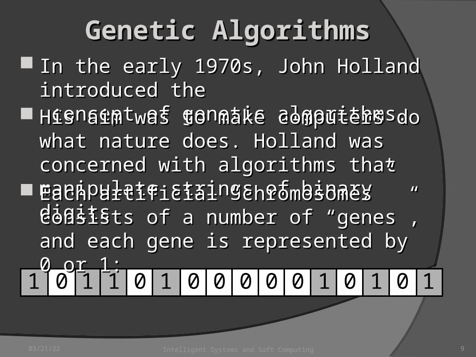
Genetic AlgorithmsGenetic Algorithms In the early 1970s, John Holland introduced the In the early 1970s, John Holland introduced the
concept of genetic algorithms. concept of genetic algorithms.
1 10 1 0 1 0 0 0 0 0 1 0 1 10
His aim was to make computers do what nature His aim was to make computers do what nature does. Holland was concerned with algorithms does. Holland was concerned with algorithms that manipulate strings of binary digits.that manipulate strings of binary digits.
Each artificial “chromosomes” consists of a Each artificial “chromosomes” consists of a number of “genes”, and each gene is represented number of “genes”, and each gene is represented by 0 or 1:by 0 or 1:
04/19/23 Intelligent Systems and Soft Computing 10
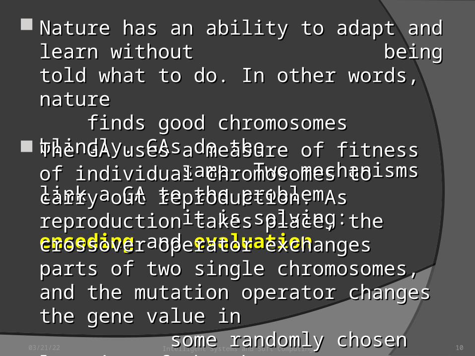
Nature has an ability to adapt and learn without Nature has an ability to adapt and learn without being told what to do. In other words, nature being told what to do. In other words, nature finds good chromosomes finds good chromosomes blindly. GAs do the same. Two blindly. GAs do the same. Two mechanisms link a GA to the problem mechanisms link a GA to the problem it is solving: it is solving: encoding encoding and and evaluationevaluation.. The GA uses a measure of fitness of individual The GA uses a measure of fitness of individual chromosomes to carry out reproduction. As chromosomes to carry out reproduction. As reproduction takes place, the crossover operator reproduction takes place, the crossover operator exchanges parts of two single chromosomes, and exchanges parts of two single chromosomes, and the mutation operator changes the gene value in the mutation operator changes the gene value in some randomly chosen location of some randomly chosen location of the chromosome.the chromosome.

04/19/23 Intelligent Systems and Soft Computing 11
Basic genetic algorithmsBasic genetic algorithms
Step 1Step 1: : Represent the problem variable domain as Represent the problem variable domain as a chromosome of a fixed length, choose a chromosome of a fixed length, choose the size of a chromosome population the size of a chromosome population NN, the crossover probability , the crossover probability ppcc and and the mutation probability the mutation probability ppmm..
Step 2Step 2: : Define a fitness function to measure the Define a fitness function to measure the performance, or fitness, of an individual performance, or fitness, of an individual chromosome in the problem domain. The fitness chromosome in the problem domain. The fitness function establishes the basis for selecting function establishes the basis for selecting chromosomes that will be mated during chromosomes that will be mated during reproduction. reproduction.
04/19/23 Intelligent Systems and Soft Computing 12
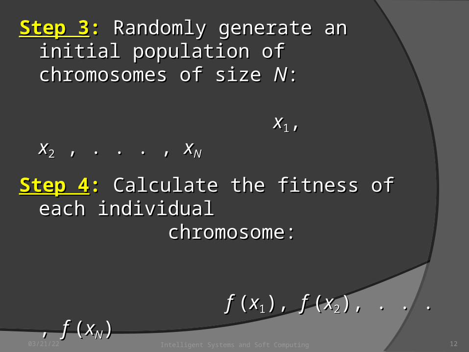
Step 3Step 3: : Randomly generate an initial population of Randomly generate an initial population of chromosomes of size chromosomes of size NN: : xx11, , xx22 , . . . , , . . . , xxNN
Step 4Step 4: : Calculate the fitness of each individual Calculate the fitness of each individual chromosome: chromosome: f f ((xx11), ), f f ((xx22), . . ), . . . , . , f f ((xxNN))
Step 5Step 5: : Select a pair of chromosomes for mating Select a pair of chromosomes for mating from the current population. from the current population. Parent chromosomes are Parent chromosomes are selected with a probability selected with a probability related to their fitness.related to their fitness.
04/19/23 Intelligent Systems and Soft Computing 13
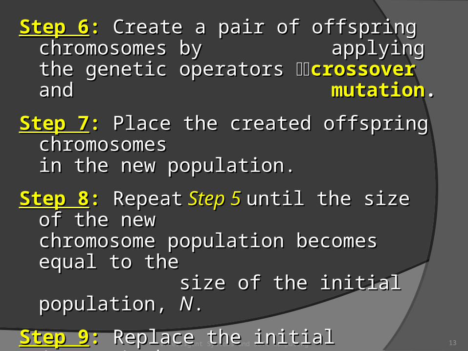
Step 6Step 6:: Create a pair of offspring chromosomes by Create a pair of offspring chromosomes by applying the genetic operators applying the genetic operators crossovercrossover and and mutationmutation..
Step 7Step 7:: Place the created offspring chromosomes Place the created offspring chromosomes in the new population. in the new population.
Step 8Step 8:: RepeatRepeat Step 5 Step 5 until the size of the new until the size of the new chromosome population becomes equal to the chromosome population becomes equal to the size of the initial population, size of the initial population, NN..
Step 9Step 9:: Replace the initial (parent) chromosome Replace the initial (parent) chromosome population with the new (offspring) population with the new (offspring) population.population.
Step 10Step 10:: Go to Go to Step 4Step 4, and repeat the process until , and repeat the process until the termination criterion is satisfied.the termination criterion is satisfied.
04/19/23 Intelligent Systems and Soft Computing 14
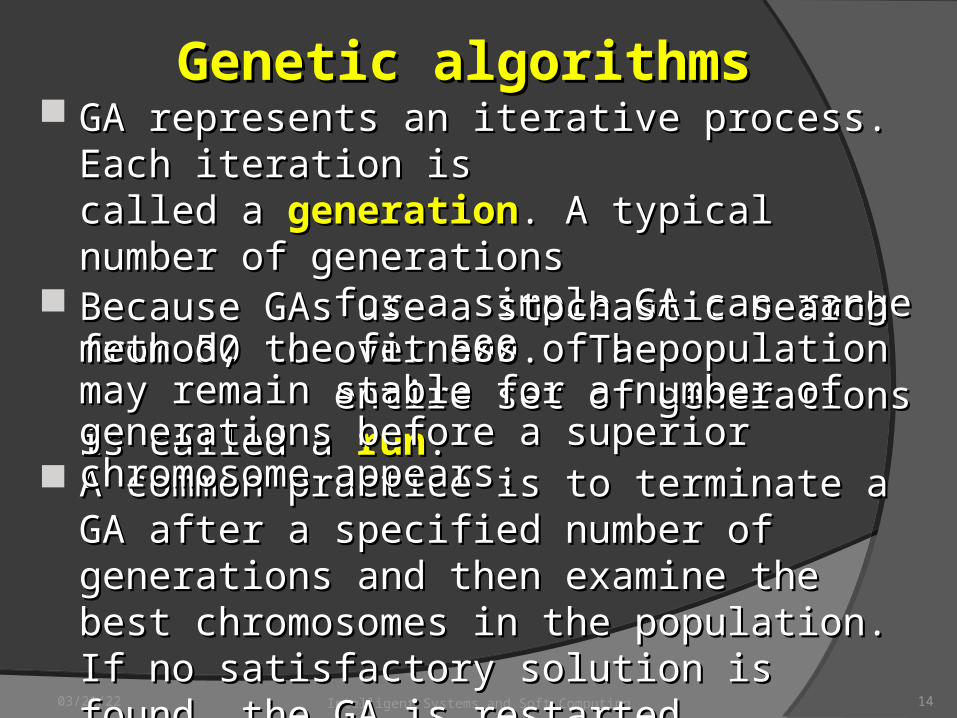
Genetic algorithmsGenetic algorithms GA represents an iterative process. Each iteration is GA represents an iterative process. Each iteration is
called a called a generationgeneration. A typical number of . A typical number of generations for a simple GA can generations for a simple GA can range from 50 to over 500. The entire range from 50 to over 500. The entire setset of generations is called a of generations is called a runrun..
A common practice is to terminate a GA after a A common practice is to terminate a GA after a specified number of generations and then examine specified number of generations and then examine the best chromosomes in the population. If no the best chromosomes in the population. If no satisfactory solution is found, the GA is restarted.satisfactory solution is found, the GA is restarted.
Because GAs use a stochastic search method, the Because GAs use a stochastic search method, the fitness of a population may remain stable for a fitness of a population may remain stable for a number of generations before a superior chromosome number of generations before a superior chromosome appears.appears.
04/19/23 Intelligent Systems and Soft Computing 15
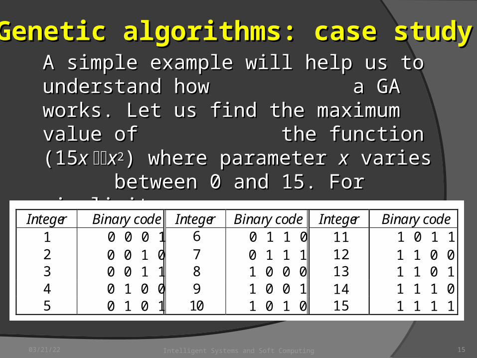
Genetic algorithms: case studyGenetic algorithms: case studyA simple example will help us to understand how A simple example will help us to understand how a GA works. Let us find the maximum value of a GA works. Let us find the maximum value of the function (15 the function (15x x xx22) where parameter ) where parameter xx varies varies between 0 and 15. For simplicity, we may between 0 and 15. For simplicity, we may assume that assume that x x takes only integer values. Thus, takes only integer values. Thus, chromosomes can be built with only four genes: chromosomes can be built with only four genes:
Integer Binary code Integer Binary code Integer Binary code1 112 7 123 8 134 9 145 10 15
6 1 0 1 11 1 0 01 1 0 11 1 1 01 1 1 1
0 1 1 00 1 1 11 0 0 01 0 0 11 0 1 0
0 0 0 10 0 1 00 0 1 10 1 0 00 1 0 1
04/19/23 Intelligent Systems and Soft Computing 16
Suppose that the size of the chromosome population Suppose that the size of the chromosome population NN is 6, the crossover probability is 6, the crossover probability ppcc equals equals 0.7, and the mutation probability 0.7, and the mutation probability ppmm equals 0.001. The fitness function in equals 0.001. The fitness function in our example is definedour example is defined byby
ff((xx) = ) = 15 15 x x – – xx22
04/19/23 Intelligent Systems and Soft Computing 17
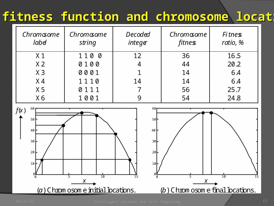
The fitness function and chromosome locationsThe fitness function and chromosome locationsChromosome
labelChromosome
stringDecodedinteger
Chromosomefitness
Fitnessratio, %
X1 1 1 0 0 12 36 16.5X2 0 1 0 0 4 44 20.2X3 0 0 0 1 1 14 6.4X4 1 1 1 0 14 14 6.4X5 0 1 1 1 7 56 25.7X6 1 0 0 1 9 54 24.8
x
50
40
30
20
60
10
00 5 10 15
f(x)
(a) Chromosome initial locations.x
50
40
30
20
60
10
00 5 10 15
(b) Chromosome final locations.
04/19/23 Intelligent Systems and Soft Computing 18
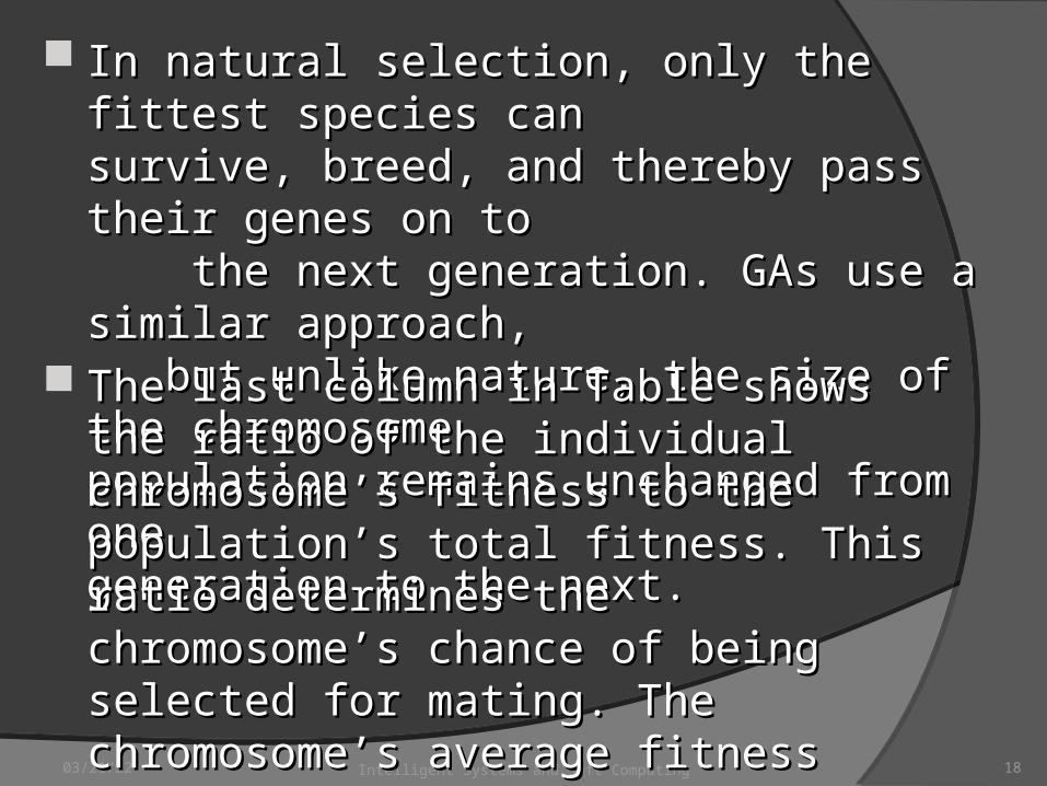
In natural selection, only the fittest species can In natural selection, only the fittest species can survive, breed, and thereby pass their genes survive, breed, and thereby pass their genes on to the next generation.on to the next generation. GAs use a GAs use a similar approach, but unlike nature, similar approach, but unlike nature, the size of the chromosome population the size of the chromosome population remains unchanged from one remains unchanged from one generation to the next.generation to the next. The last column in Table shows the ratio of the The last column in Table shows the ratio of the individual chromosome’s fitness to the individual chromosome’s fitness to the population’s total fitness. This ratio determines population’s total fitness. This ratio determines the chromosome’s chance of being selected for the chromosome’s chance of being selected for mating. The chromosome’s average fitness mating. The chromosome’s average fitness improves from one generation to the next.improves from one generation to the next.
04/19/23 Intelligent Systems and Soft Computing 19
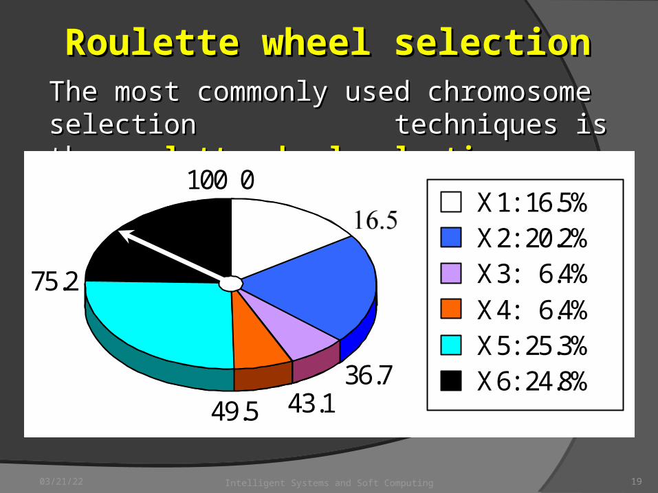
Roulette wheel selectionRoulette wheel selectionThe most commonly used chromosome selection The most commonly used chromosome selection techniques is the techniques is the roulette wheel selectionroulette wheel selection..
100 0
36.743.149.5
75.2
X1: 16.5%X2: 20.2%X3: 6.4%X4: 6.4%X5: 25.3%X6: 24.8%
04/19/23 Intelligent Systems and Soft Computing 20
CrossoverCrossover operatoroperator In our example, we have an initial population of 6 In our example, we have an initial population of 6
chromosomes. Thus, to establish the same chromosomes. Thus, to establish the same population in the next generation, the population in the next generation, the roulette wheel would be roulette wheel would be spun six times. spun six times. Once a pair of parent chromosomes is selected, Once a pair of parent chromosomes is selected, the the crossovercrossover operator is applied.operator is applied.
04/19/23 Intelligent Systems and Soft Computing 21
First, the crossover operator randomly chooses a First, the crossover operator randomly chooses a crossover point where two parent crossover point where two parent chromosomes “break”, and then chromosomes “break”, and then exchanges the chromosome exchanges the chromosome parts after that point. As a result, two new parts after that point. As a result, two new offspring are created. offspring are created. If a pair of chromosomes does not cross over, If a pair of chromosomes does not cross over, then the chromosome cloning takes place, and the then the chromosome cloning takes place, and the offspring are created as exact copies of each offspring are created as exact copies of each parent.parent.
04/19/23 Intelligent Systems and Soft Computing 22
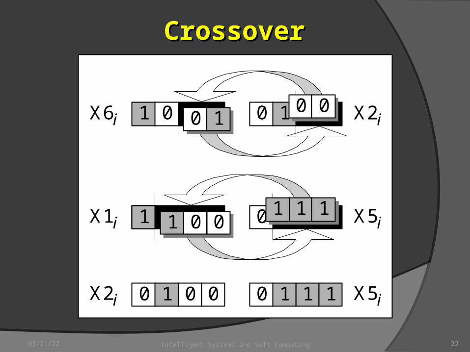
CrossoverCrossover
X6i 1 00 0 01 0 X2i
0 01 0X2i 0 11 1 X5i
0X1i 0 11 1 X5i1 01 0
0 10 0
11 101 0
04/19/23 Intelligent Systems and Soft Computing 23
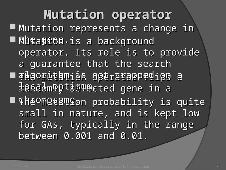
Mutation operatorMutation operator Mutation represents a change inMutation represents a change in the gene.the gene.
The mutation probability is quite small in nature, The mutation probability is quite small in nature, and is kept low for GAs, typically in the range and is kept low for GAs, typically in the range between 0.001 and 0.01.between 0.001 and 0.01.
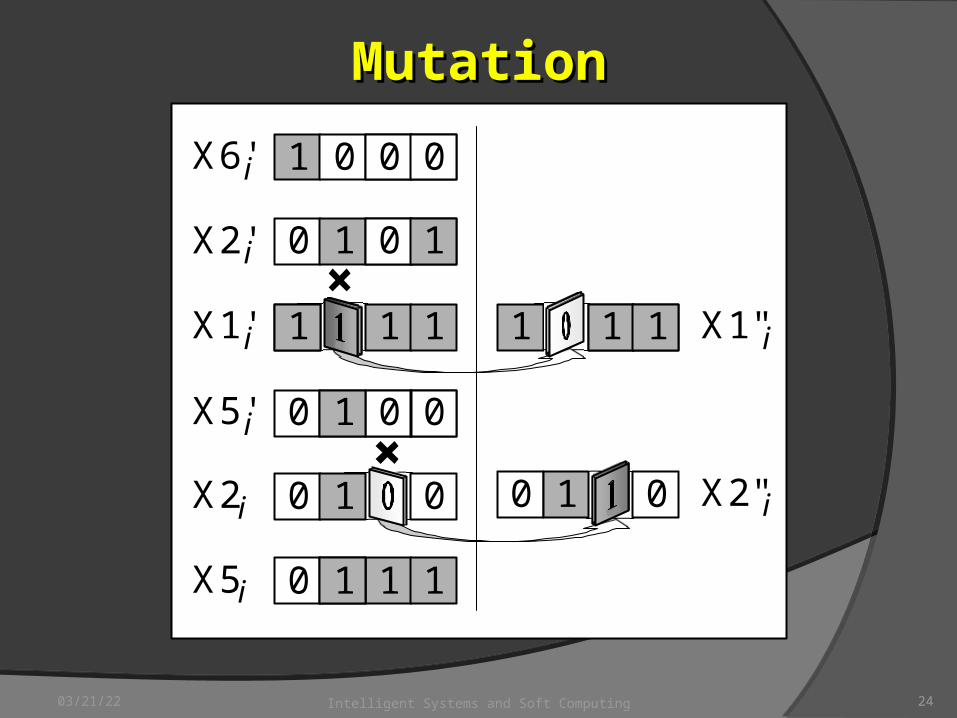
The mutation operator flips a randomly selected The mutation operator flips a randomly selected gene in a chromosome.gene in a chromosome.
Mutation is a background operator. Its role is to Mutation is a background operator. Its role is to provide a guarantee that the search algorithm is provide a guarantee that the search algorithm is not trapped on a local optimum.not trapped on a local optimum.
04/19/23 Intelligent Systems and Soft Computing 24
MutationMutation
0 11 1X5'i 01 0
X6'i 1 00
0 01 0X2'i 0 1
0 0
0 1 111X5i
1 1 1 X1"i1 1
X2"i0 1 0
0X1'i 1 1 1
0 1 0X2i
04/19/23 Intelligent Systems and Soft Computing 25
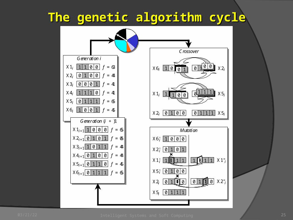
The genetic algorithm cycleThe genetic algorithm cycle
1 01 0X1i
Generation i
0 01 0X2i
0 00 1X3i
1 11 0X4i
0 11 1X5i f = 56
1 00 1X6i f = 54
f = 36
f = 44
f = 14
f = 14
1 00 0X1i+1
Generation (i + 1)
0 01 1X2i+1
1 10 1X3i+1
0 01 0X4i+1
0 11 0X5i+1 f = 54
0 11 1X6i+1 f = 56
f = 56
f = 50
f = 44
f = 44
Crossover
X6i 1 00 0 01 0 X2i
0 01 0X2i 0 11 1 X5i
0X1i 0 11 1 X5i1 01 0
0 10 0
11 101 0
Mutation
0 11 1X5'i 01 0
X6'i 1 00
0 01 0X2'i 0 1
0 0
0 1 111X5i
1 1 1 X1"i1 1
X2"i0 1 0
0X1'i 1 1 1
0 1 0X2i
04/19/23 Intelligent Systems and Soft Computing 26
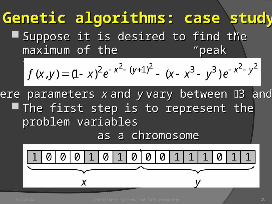
Genetic algorithms: case studyGenetic algorithms: case study Suppose it is desired to find the maximum of the Suppose it is desired to find the maximum of the
“peak” function of two variables: “peak” function of two variables:
The first step is to represent the problem variables The first step is to represent the problem variables as a chromosome as a chromosome parameters parameters x x and and y y as a concatenated as a concatenated binary string:binary string:
2222)()1(),( 33)1(2 yxyx eyxxexyxf
1 00 0 1 10 0 0 10 1 1 10 1
yx
where parameters where parameters x x and and y y vary between vary between 3 and 3.3 and 3.
04/19/23 Intelligent Systems and Soft Computing 27
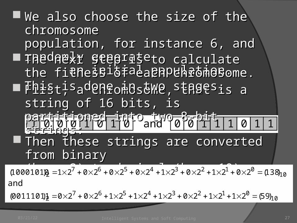
We also choose the size of the chromosome We also choose the size of the chromosome population, for instance 6, and randomly population, for instance 6, and randomly generate an initial population.generate an initial population.
Then these strings are converted from binary Then these strings are converted from binary (base 2) to decimal (base 10): (base 2) to decimal (base 10):
1 00 0 1 10 0 0 10 1 1 10 1and
1001234567
2 )138(2021202120202021)10001010( and
1001234567
2 )59(2121202121212020)00111011(
First, a chromosome, that is a string of 16 bits, is First, a chromosome, that is a string of 16 bits, is partitioned into two 8-bit strings:partitioned into two 8-bit strings:
The next step is to calculate the fitness of each The next step is to calculate the fitness of each chromosome. This is done in two stages.chromosome. This is done in two stages.
04/19/23 Intelligent Systems and Soft Computing 28
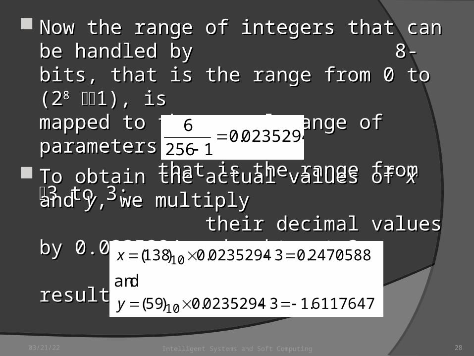
Now the range of integers that can be handled by Now the range of integers that can be handled by 8-bits, that is the range from 0 to (2 8-bits, that is the range from 0 to (288 1), 1), is mapped to the actual range of is mapped to the actual range of parameters parameters x x and and yy, that is the , that is the range from range from 3 to 3:3 to 3:
To obtain the actual values of To obtain the actual values of x x and and yy, we multiply , we multiply their decimal values by their decimal values by 0.0235294 and subtract 3 from 0.0235294 and subtract 3 from the results:the results:
0235294.01256
6
2470588.030235294.0)138( 10 x
and6117647.130235294.0)59( 10 y
04/19/23 Intelligent Systems and Soft Computing 29
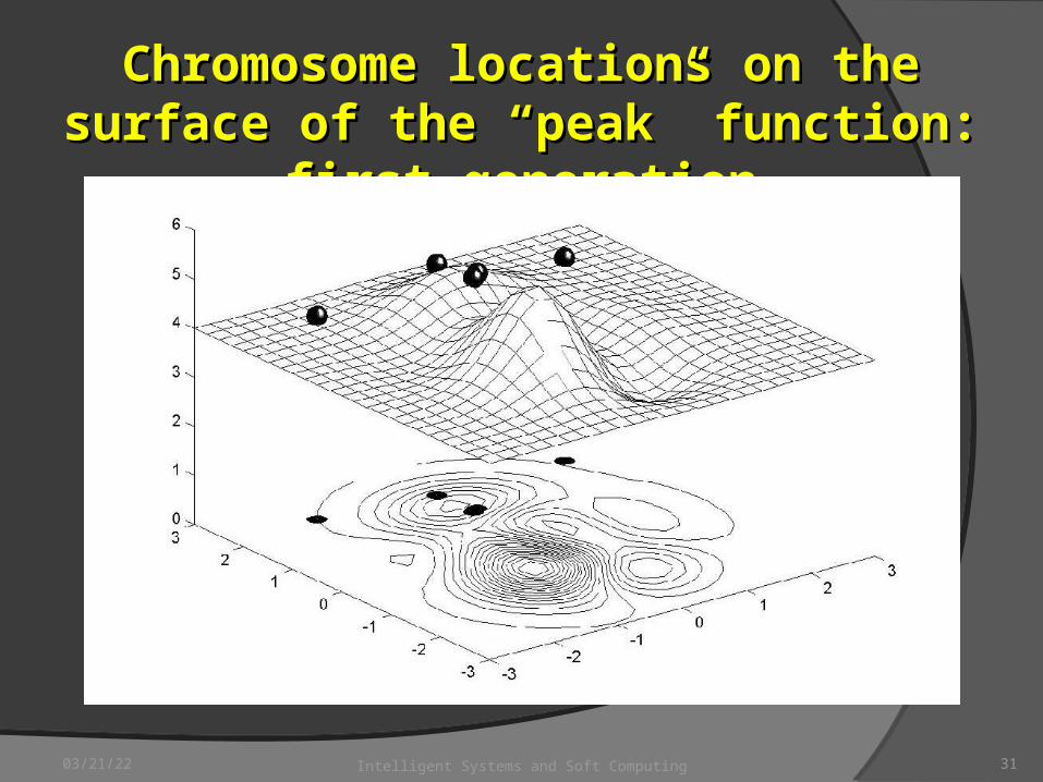
Using decoded values of Using decoded values of x x and and y y as inputs in the as inputs in the mathematical function, the GA calculates mathematical function, the GA calculates the fitness of each the fitness of each chromosome.chromosome. To find the maximum of the “peak” function, we To find the maximum of the “peak” function, we will use crossover with the probability equal to 0.7 will use crossover with the probability equal to 0.7 and mutation with the probability equal to 0.001. and mutation with the probability equal to 0.001. As we mentioned earlier, a common practice in As we mentioned earlier, a common practice in GAs is to specify the number of generations. GAs is to specify the number of generations. Suppose the desired number of generations is 100. Suppose the desired number of generations is 100. That is, the GA will create 100 generations of 6 That is, the GA will create 100 generations of 6 chromosomes before stopping. chromosomes before stopping.
04/19/23 Intelligent Systems and Soft Computing 30
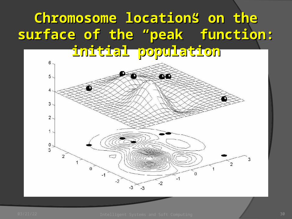
Chromosome locations on the surface of the Chromosome locations on the surface of the “peak”“peak” function: initial populationfunction: initial population
04/19/23 Intelligent Systems and Soft Computing 31
Chromosome locations on the surface of the Chromosome locations on the surface of the “peak”“peak” function: first generationfunction: first generation
04/19/23 Intelligent Systems and Soft Computing 32
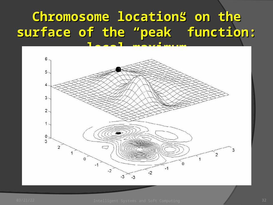
Chromosome locations on the surface of the Chromosome locations on the surface of the “peak” function: local maximum“peak” function: local maximum
04/19/23 Intelligent Systems and Soft Computing 33
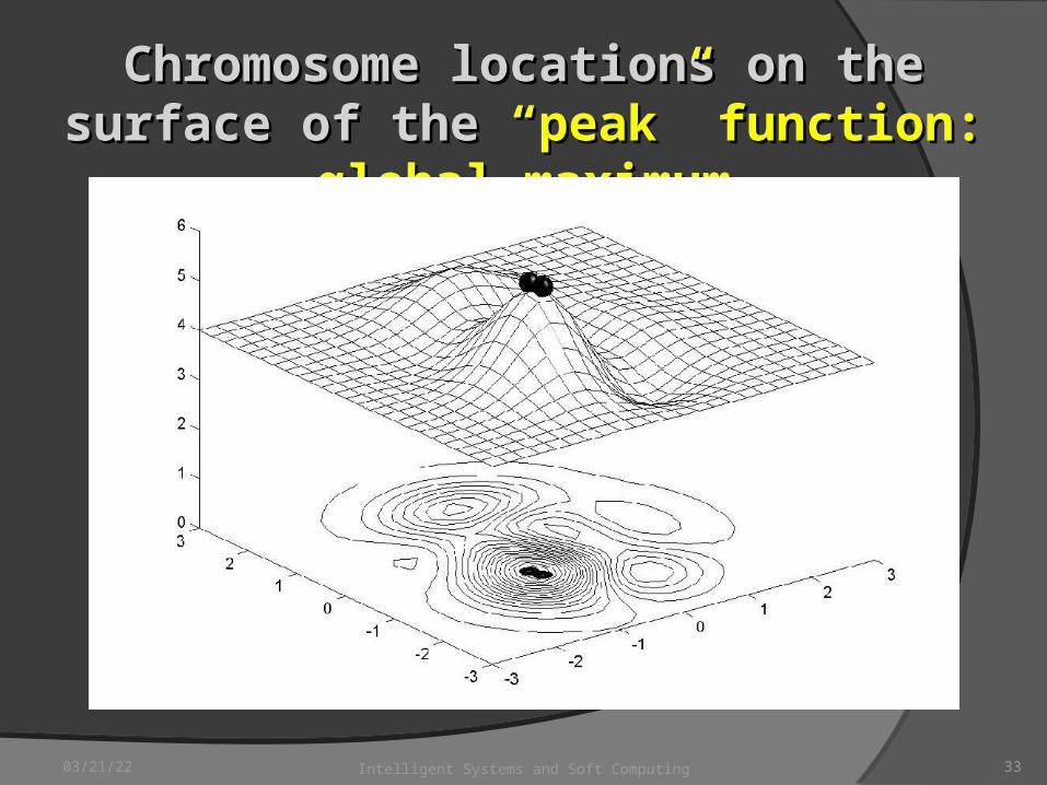
Chromosome locations on the surface of the Chromosome locations on the surface of the “peak” function: global maximum“peak” function: global maximum
04/19/23 Intelligent Systems and Soft Computing 34
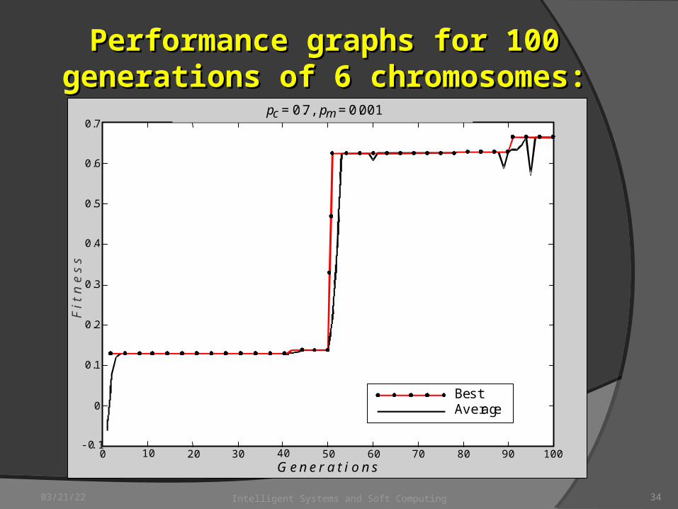
Performance graphs for 100 generations of 6 Performance graphs for 100 generations of 6 chromosomes: local maximumchromosomes: local maximum
pc = 0.7, pm = 0.001
G e n e r a t i o n s
BestAverage
80 90 10060 7040 5020 30100-0.1
0.5
0.6
0.7
0
0.1
0.2
0.3
0.4
F i
t n e
s s
04/19/23 Intelligent Systems and Soft Computing 35
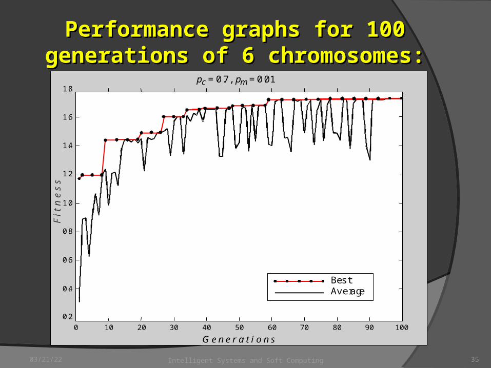
Performance graphs for 100 generations of 6 Performance graphs for 100 generations of 6 chromosomes: global maximumchromosomes: global maximum
BestAverage
100
G e n e r a t i o n s80 9060 7040 5020 3010
pc = 0.7, pm = 0.011.8
0
0.2
0.4
0.6
0.8
1.0
1.2
1.4
1.6
F i
t n e
s s
04/19/23 Intelligent Systems and Soft Computing 36
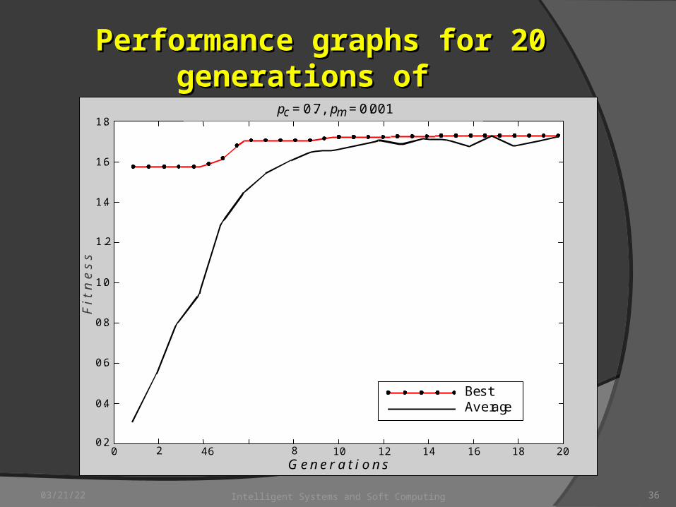
Performance graphs for 20 generations of Performance graphs for 20 generations of 60 chromosomes60 chromosomes
pc = 0.7, pm = 0.001
BestAverage
20G e n e r a t i o n s
16 1812 148 1046200.2
0.4
0.6
0.8
1.0
1.2
1.4
1.6
1.8
F i
t n e
s s
04/19/23 Intelligent Systems and Soft Computing 37
Case study: maintenance schedulingCase study: maintenance scheduling Maintenance scheduling problems are usually Maintenance scheduling problems are usually
solved using a combination of search solved using a combination of search techniques and heuristics.techniques and heuristics.
These problems are complex and difficult to These problems are complex and difficult to solve. solve.
They are NP-complete and cannot be solved by They are NP-complete and cannot be solved by combinatorial search techniques. combinatorial search techniques.
Scheduling involves competition for limited Scheduling involves competition for limited resources, and is complicated by a great resources, and is complicated by a great number of badly formalised number of badly formalised constraints.constraints.
04/19/23 Intelligent Systems and Soft Computing 38
1. Specify the problem, define constraints and 1. Specify the problem, define constraints and
optimum criteria; optimum criteria;
2. Represent the problem domain as a 2. Represent the problem domain as a
chromosome; chromosome;
3.3. Define a fitness function to evaluate the Define a fitness function to evaluate the
chromosome performance;chromosome performance;
4. Construct the genetic operators;4. Construct the genetic operators;
5. Run the GA and tune its parameters.5. Run the GA and tune its parameters.
Steps in the GA developmentSteps in the GA development
04/19/23 Intelligent Systems and Soft Computing 39
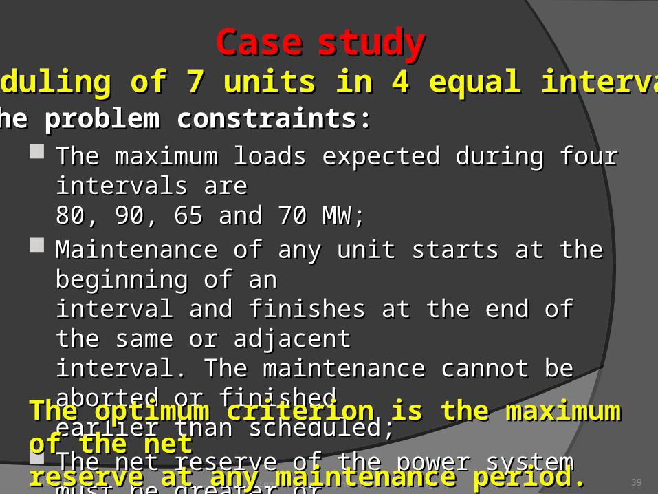
CaseCase studystudyScheduling of 7 units in 4 equal intervalsScheduling of 7 units in 4 equal intervals
The maximum loads expected during four intervals are The maximum loads expected during four intervals are 80, 90, 65 and 70 MW; 80, 90, 65 and 70 MW;
Maintenance of any unit starts at the beginning of an Maintenance of any unit starts at the beginning of an interval and finishes at the end of the same or interval and finishes at the end of the same or adjacent interval. The maintenance cannot be adjacent interval. The maintenance cannot be aborted or finished earlier than scheduled;aborted or finished earlier than scheduled;
The net reserve of the power system must be greater or The net reserve of the power system must be greater or equal to zero at any interval. equal to zero at any interval.
The optimum criterion is the maximum of the net The optimum criterion is the maximum of the net reserve at any maintenance period. reserve at any maintenance period.
The problem constraints:The problem constraints:
04/19/23 Intelligent Systems and Soft Computing 40
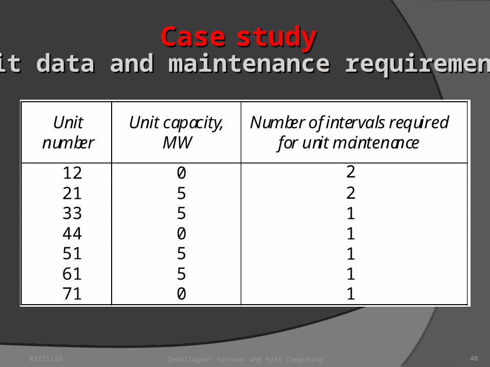
Unit data and maintenance requirementsUnit data and maintenance requirements
Unitnumber
Unit capacity,MW
Number of intervals requiredfor unit maintenance
12 0 221111
21 533 544 051 561 571 0 1
CaseCase studystudy
04/19/23 Intelligent Systems and Soft Computing 41
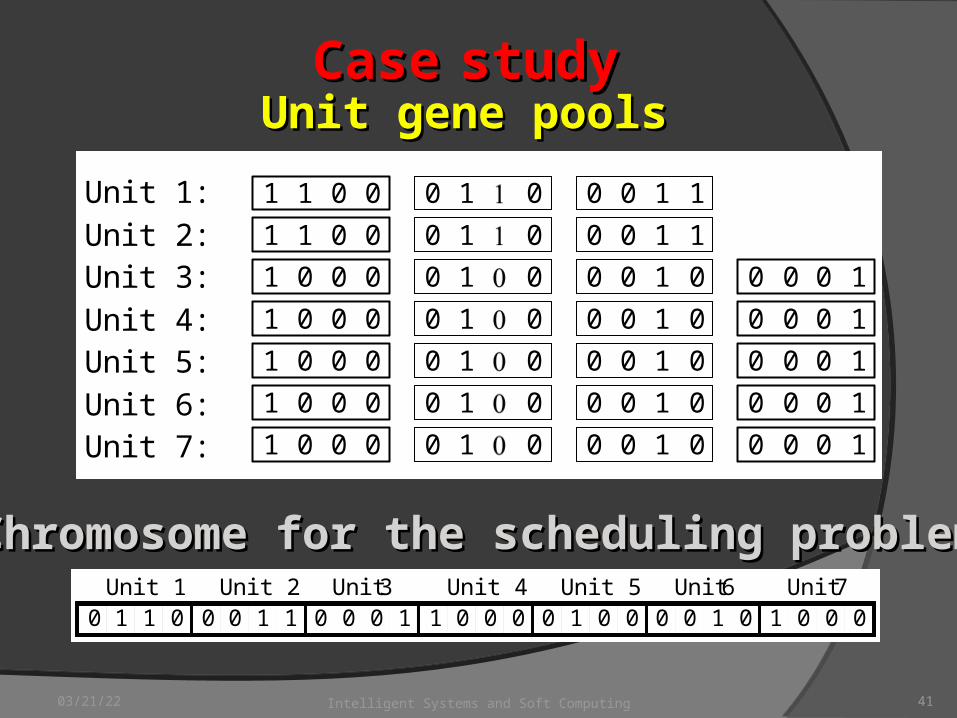
Unit gene poolsUnit gene pools
Chromosome for the scheduling problemChromosome for the scheduling problem
Unit 1: 1 01 0 0 1 0 0 10 1
Unit 2: 1 01 0 0 1 0 0 10 1
Unit 3: 1 00 0 0 1 0 0 10 0 0 00 1
Unit 4: 1 00 0 0 1 0 0 10 0 0 00 1
Unit 5: 1 00 0 0 1 0 0 10 0 0 00 1
Unit 6: 1 00 0 0 1 0 0 10 0 0 00 1
Unit 7: 1 00 0 0 1 0 0 10 0 0 00 1
0 11 0 0 10 1 0 00 1 1 00 0 0 01 0 0 10 0 1 00 0Unit 1 Unit 3Unit 2 Unit 4 Unit 6Unit 5 Unit 7
CaseCase studystudy
04/19/23 Intelligent Systems and Soft Computing 42
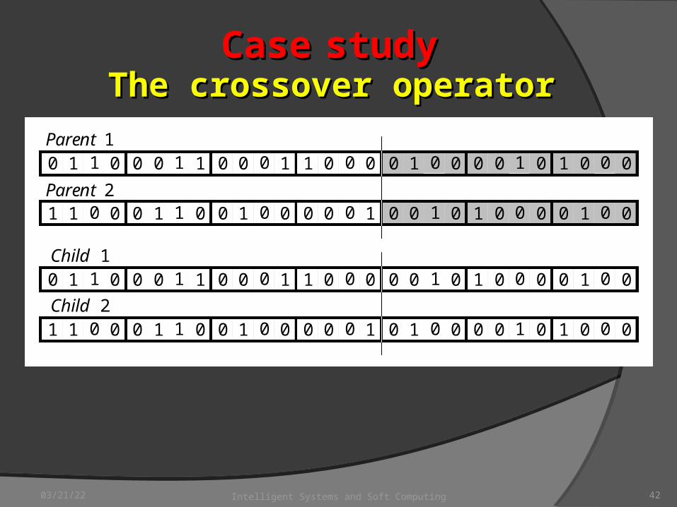
The crossover operatorThe crossover operator
0 11 0 0 10 1 0 00 1 1 00 0 0 01 0 0 10 0 1 00 0Parent 1
1 01 0 0 11 0 0 01 0 0 00 1 0 10 0 1 00 0 0 01 0Parent 2
0 11 0 0 10 1 0 00 1 1 00 0 0 10 0 1 00 0 0 01 0Child 1
1 01 0 0 11 0 0 01 0 0 00 1 0 01 0 0 10 0 1 00 0Child 2
CaseCase studystudy
04/19/23 Intelligent Systems and Soft Computing 43
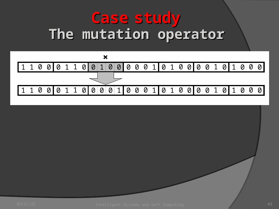
The mutation operatorThe mutation operator
1 01 0 0 11 0 0 010 0 00 1 0 01 0 0 10 0 1 00 00 01 0
1 01 0 0 11 0 0 010 0 00 1 0 01 0 0 10 0 1 00 00 00 1
CaseCase studystudy
04/19/23 Intelligent Systems and Soft Computing 44
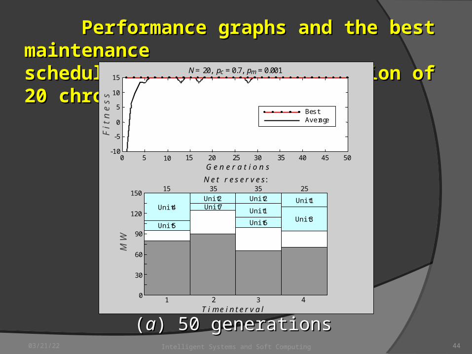
Performance graphs and the best maintenance Performance graphs and the best maintenance schedules created in a population of 20 schedules created in a population of 20 chromosomeschromosomes
((aa) 50 generations) 50 generations
0
30
60
90
120
150Unit 2 Unit 2Unit 7
Unit 1
Unit 6
Unit 1
Unit 3Unit 5
Unit 4
1 2 3 4T i m e i n t e r v a l
N e t r e s e r v e s:15 35 35 25
N = 20, pc = 0.7, pm = 0.001
BestAverage
5 15 25 3510 3020 40 45 500-10
-5
0
5
10
15
G e n e r a t i o n s
F i
t n e
s s
M W
04/19/23 Intelligent Systems and Soft Computing 45
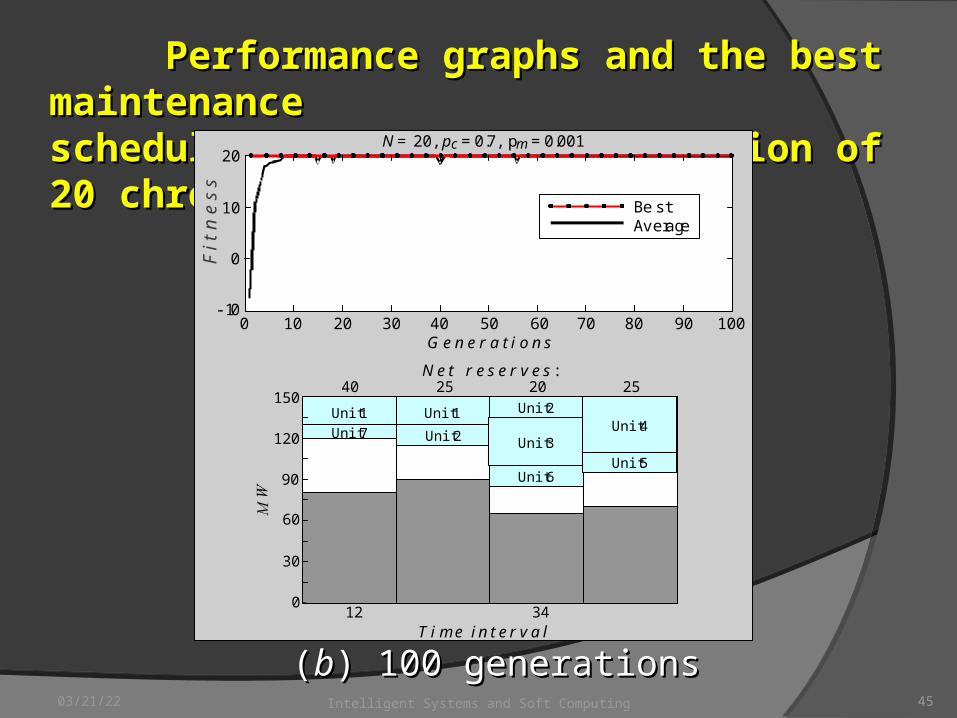
((bb) 100) 100 generationsgenerations
Performance graphs and the best maintenance Performance graphs and the best maintenance schedules created in a population of 20 schedules created in a population of 20 chromosomeschromosomes
G e n e r a t i o n s
0
30
60
12 34T i m e i n t e r v a l
N e t r e s e r v e s :40 25 20 25
Unit 2
Unit 2
Unit 7
Unit 1
Unit 6
Unit 1
Unit 3
Unit 5
Unit 4
90
120
150
N = 20, pc = 0.7, pm = 0.001
Be stAverage
10 30 50 70200 6040 80 90 100-10
0
10
20
G e n e r a t i o n s
F i
t n e
s s
04/19/23 Intelligent Systems and Soft Computing 46
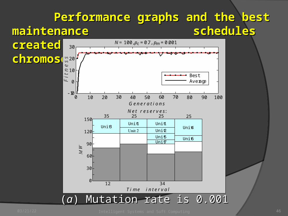
Performance graphs and the best maintenance Performance graphs and the best maintenance schedules created in a population of 100 schedules created in a population of 100 chromosomeschromosomes
((aa) Mutation rate is 0.001) Mutation rate is 0.001
12 34T i m e i n t e r v a l
35 25 25 25
Unit 2
Unit 7
Unit 1
Unit 6
Unit 1Unit 3
Unit 5
Unit 4
0
30
60
90
120
150
N = 100, pc = 0.7, pm = 0.001
G e n e r a t i o n s
N e t r e s e r v e s:
BestAverage
10 30 50 70200 6040 80 90 100-10
0
10
20
30
F i
t n e
s s
04/19/23 Intelligent Systems and Soft Computing 47
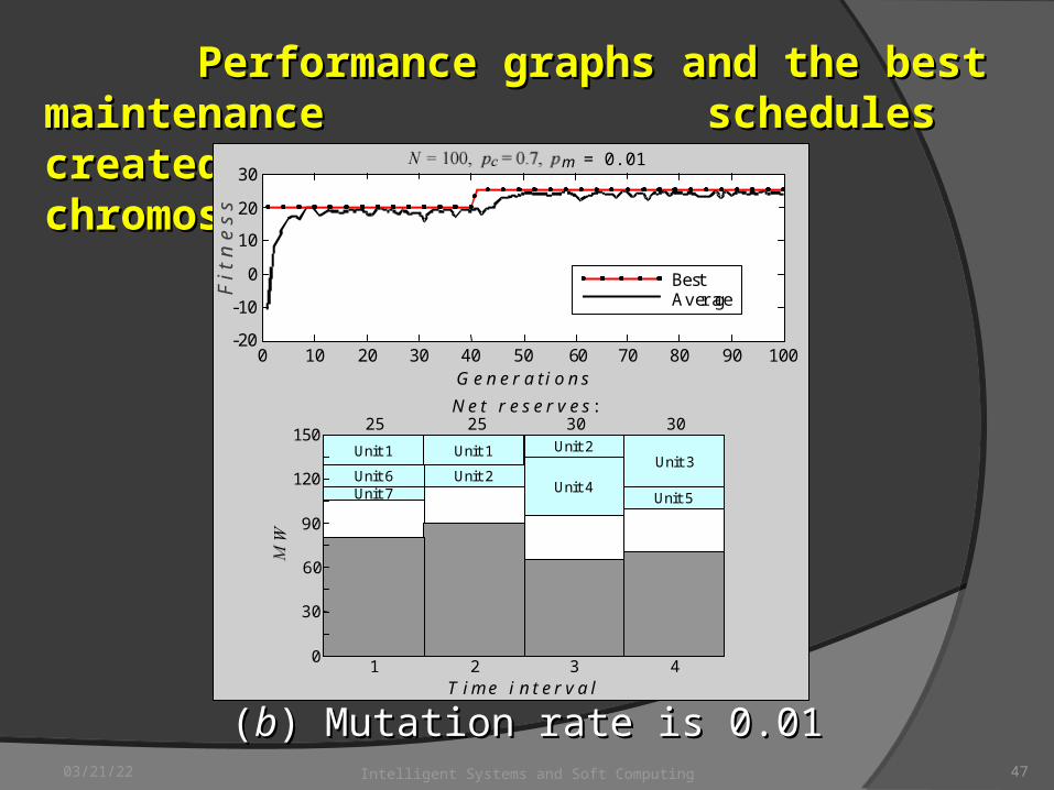
((bb) Mutation rate is 0.01) Mutation rate is 0.01
Performance graphs and the best maintenance Performance graphs and the best maintenance schedules created in a population of 100 schedules created in a population of 100 chromosomeschromosomes
1 2 3 4T i m e i n t e r v a l
N e t r e s e r v e s :25 25 30 30
Unit 2
Unit 2
Unit 7Unit 6
Unit 1Unit 3
Unit 5Unit 4
0
30
60
90
120
150Unit 1
N = 100, c = 0.7, m = 0.01
G e n e r a t i o n s10 30 50 70200 6040 80 90 100
BestAverage
-20
-10
0
10
30
20F
i t n
e s
s