Embed Size (px)
Citation preview

DESIGN, CONSTRUCTION AND YIELD
ANALYSIS OF A 1.2KW STANDALONE
PHOTOVOLTAIC SYSTEM
by
Rajneel S. Prasad
A thesis submitted in partial fulfilment of the
requirements for the degree of Master of Science in Physics
Copyright © 2013 by Rajneel S. Prasad
School of Engineering and Physics
Faculty of Science, Technology and Environment
The University of the South Pacific
Fiji
August 2013

Declaration of Originality
I, Rajneel S. Prasad, hereby declare that this thesis is my original work and wherever
the work of others has been used, it has been clearly referenced.
Signature
Date 24th May, 2013
Name Rajneel S. Prasad
Student ID S11023961
Statement by Principal Supervisor
The research in this thesis was performed under my supervision and to my
knowledge is the sole work of Mr Rajneel S. Prasad.
Signature
Date 24th May, 2013
Name Dr. Atul Raturi
Designation Principal Supervisor
Statement by Co Supervisor
The research in this thesis was performed under my supervision and to my
knowledge is the sole work of Mr Rajneel S. Prasad.
Signature
Date 24th May, 2013
Name Dr. R. Corkish
Designation Co Supervisor

i
Acknowledgments The successful compilation of this thesis would not have been possible through the
assistance, support and guidance of many individuals who have helped me
throughout my research work. Therefore, I would like to take this opportunity to
express my sincere gratitude and heartfelt appreciation to the following individuals
whose help has been very much appreciated.
Firstly, I would like to express profound gratitude to my supervisor, Dr. Atul Raturi,
for his invaluable support, encouragement, supervision and useful suggestions
throughout this research work. My sincere gratitude is also due to Dr. R. Corkish, my
co-supervisor, for providing his help wherever needed. My sincere appreciation also
goes to the technical staff of School of Engineering and Physics; Mr. Amit Deo, Mr.
Abhinay Shandil, Mr. Joape Cawanibuka, Mr. Neil Singh, Mr. Rohit Lal, Mr. Shanil
Deo and Mr. Viti Buadromo for helping me during the experimental stages of my
thesis especially the technical assistance with operation of the instruments. My
special thanks also go to Mr. Adish Naidu, Mr. Kalivati Artack and the technical and
maintenance team from USP Properties and Maintenance Division for providing me
with the necessary equipment and instruments. Special thanks also go to my dear
friends; Mr. Shivneel Prasad, Ms. Pritika, Mr. Naveendra Reddy, Ms Monishka
Narayan, Mr. Pranil Singh, Ms Priti Maharaj, Ms Esha Chetty, Ms. Pritika Reddy,
Mr. Malvin Nadan, Mr. Atesh Gosai, Mr. Aman Deo, Mr. Sunil Chand, Mr Ravin
Prasad and Ms Bianca Kumar and Mr. Imraan Jannif for the words of encouragement
and support during every stage of my thesis. My sincere thanks also goes to the staff
of Fiji Meteorological service specially to Mr and Mrs Funaki, Mr Alipate
Waqaniculua, Mr Shalvin Singh, Mr Sanjay Prakash, Mr Amit Singh, Mr Rajneel
Prasad, Mr Steven Meke, Mr Samisoni Waqavakatonga, Mr Saki Rabitu, Ms Aditi
Sharan and Mr Leonard Bale.
Finally, I would like to thank my mum, for her continuous support throughout my
life and always encouraging me to further my knowledge and studies. Thanks also to
my sisters, Shariya, Komal and Asnita and my brother Roneel.

ii
The funding for construction of the PV system studied in this work was provided to
the Principal supervisor by the US government through the Regional Environment
Office, US Embassy, Suva.
iii
Abstract
Photovoltaic (PV) energy generation is in continuous increase round the globe due to
fossil fuel depletion, fuel price hikes and the need for energy generation from cleaner
sources. Moreover, sometimes PV energy generation is the only feasible alternative
to supply electricity in remote areas which are separated by long distances and ocean.
The main objective of the study is to design, construct and monitor two optimum
stand-alone photovoltaic (SAPV) systems that can satisfy lighting and laptop
charging demands of the student fales1. The study aims to verify the actual
performance of the designed SAPV systems with the simulated performance results.
This study also intends to provide SAPV system performance data for Fiji and
develop a pathway for future SAPV systems by providing SAPV system
performance data under field conditions. Furthermore, a sensitivity analysis was
carried out to determine the future prospects of SAPV system under varying
economical, environment and operating conditions.
The SAPV system was designed using HOMERTM, Solar Design Studio 6.0TM and
PV systTM, and the SAPV component performance data of inverter, charge controller,
battery and PV module was obtained by using standard SAPV component testing
procedures. In designing an optimum SAPV system, a complete solar resource
assessment was carried out using 10 years meteorological data and the shading
patterns within the vicinity of the fales. The performance of the SAPV system was
monitored by a DELL computer and CR23X datalogger at the project site.
The optimal orientation of the SAPV system are 15-20° tilt and 330-350° azimuth
from true north with annual solar access of 90.3% to direct radiation on a clear day.
For both the SAPV systems, the monthly average daily final yield (Yf) and
performance ratio (PR) range from 3.5-4.2 kWh/kWp and 65.4-81.3% respectively.
1 A fale or a bure is a traditional Fijian meeting place. At USP a numbers of fales to had been built to
serve as student study areas.
iv
The internal rate of return (IRR) of the lighting system is 1.5% and for the laptop
charging system is 1.3%. Based on 2010 pricing of PV components, the levelized
costs of energy (LCOE) are $0.96/kWh and $1.05/kWh for light and laptop system
respectively. The payback times for the two systems are 22.4 and 22.7 years
considering the relatively low cost of electricity in Fiji. The actual performance
analysis of SAPV system (each 625Wp) shows that the normalized annual energy
delivered to the load from light and laptop systems are 761.1 kWh/year and 779.4
kWh/year respectively.
Eight dimensional sensitivity analysis of economic feasibility based on initial system
cost and environmental parameters that drive the energy generation delineates that
LCOE is a strong function of initial capital cost and global radiation at the project
site. The sensitivity analysis shows the pathways that would make SAPV system
competitive in the energy generation market in Fiji.

v
List of Abbreviations, Units and Nomenclature
LIST OF ABBREVIATIONS
3D Three dimension
AGM Absorption Glass Mat
AM Air mass
AS/NZS Australia and New Zealand Standard
ASTM American Society of Testing and Materials
CPV concentrated photovoltaic cell
DOE Department of Energy
DOD Depth Of Discharge
Ec conduction band
EE Energy Efficiency
EMA Environment Management Act
ENSO El’Nino Southern Oscillation
EV valence band
FDoE Fiji Department of Energy
FEA Fiji Electricity Authority
FSM Federated States of Micronesia
GIS Geographic Information System
GPS Global Positioning System
HIT Heterojunction with Intrinsic Thin layer
IOD Indian Ocean Dipole
IEC International Energy Centre
IEEE Institute of Electrical and Electronics Engineers
IRR Internal Rate of Return
LOCE Levelized Cost of Energy
LOLP Loss of Load Probability
MAD mean-absolute-difference
MPP Maximum Power Point

vi
MPPT Maximum Powers Point Tracker
NASA National Aeronautics and Space Administration
NEP National Energy Planning
NPC Net Present Cost
NREL National Renewable Energy Laboratory
PIC Pacific Island Countries
PNG Papua New Guinea
PV Photovoltaic
REP Renewable Energy Program
RESCO Renewable Energy Service Companies
RMSD Root-mean-square-difference
SAPV Stand-alone Photovoltaic system
SCADA Supervisory Control And Data Acquisition
SOC State Of Charge
SOI Southern Oscillation Index
SPCZ South Pacific Convergence Zone
SRC Standard Reporting Condition
STC Standard Reporting Condition
THD Total Harmonic Distortion
TDR Transmission, Distribution and Retail
USP University of the South Pacific
VRLA Valve Regulated Lead Acid
LIST OF UNITS
A Ampere
Ah Amp Hour
cm Centimetres
GW Gigawatt
GWh Gigawatt-Hour
hrs Hours
J Joule
km Kilometre

vii
kV Kilovolt
kW Kilowatt
kWp Kilowatt Peak
K Kelvin
m Meter
m/s Meters per Second
MW Megawatt
nm Nanometres
TW Terawatt
TWh Terawatt-Hour
V Volts
W Watt
Wm-2 Watts per Meter Squared
% Percent
$ Dollars
μs Microsecond
° Degree
°C Degrees Celcius
μm Micrometre
LIST OF NOMENCLATURE
EIn Energy In
EOut Energy Out
EStored Energy Stored
Gb Beam radiation
Gd Diffuse radiation
GT Global radiation
f Horizon factor
fPV PV derating factor
FF Fill Factor
G Radiation
I Current
viii
Impp Maximum Power Point Current
Isc Short circuit current
Lu Unused energy
Ls System loss
P Power
PAC AC power
PDC DC power
PL Power lost
Pmpp Maximum Power Point Power
Pown DC loss in inverter
rohm Ohmic loss in the coils and wires
T Temperature
Tc Cell temperature.
Vmpp Maximum Power Point Voltage
Voc Open circuit voltage
Ya PV Array Production
Yf Final yield
YPV PV array rated capacity
Yu Normalized potential PV production
νSwitch Semiconductor switch loss
αp Temperature coefficient of power
β Surface slope
ρg Ground reflectance or albedo
τA Aerosol optical depth � Efficiency
ix
Table of Contents
Acknowledgments i
Abstract iii
List of abbreviations, units and nomenclature v
Table of contents ix
List of Figures xiv
List of tables xix
Chapter 1 21
1.0 Introduction and Literature Review 21
1.1 Fiji Islands 21
1.2 Energy Situation in the Pacific 22
1.3 Fijis Energy Situation 24
1.4 Renewable Energy and Fiji Government 26
1.5 FEA 27
1.6 Motivation of this project 29
1.7 Review of SAPV System Design Method 30
1.8 Review of SAPV System Performance 32
CHAPTER 2 34
2.0 Background 34
2.1 Sun 34
2.2 Solar spectrum. 35
2.3 PV module technology 36
2.4 Operation of PV modules P-N junction 38
2.5 Efficiency 41
x
2.6 Photovoltaic array interconnections 42
2.7 SAPV and Grid PV system. 43
2.8 Photovoltaic market status 45
2.9 Existing Photovoltaic System. 47
CHAPTER 3 50
3.0 Solar resource Assessment 50
3.1 Solar resource 50
3.2 Solar radiation variability 52
3.3 Solar resource assessment 53
3.4 Solar resource assessment method. 55
3.4.1 Instrumentation 55
3. 4.1 Solar Radiation Data Correction. 56
3.4.2 Site Specific Solar resource assessment. 57
3.4.3 Optimum tilt and azimuth 58
3.5. Results and Discussions 59
3.5.1 Solar radiation data correction 59
3.5.2 Site selection and resource assessment 64
3.5.3 Optimum tilt and azimuth 66
3.6 Conclusion 69
CHAPTER 4 70
4.0 Performance testing and monitoring. 70
4.1 Introduction 70
4.2 Inverters 71
4.2.1 Inverter Testing 72
4.22 Calculation of inverter efficiency. 74
4.23 Inverter performance monitoring and control. 76
4.24 Component Results and discussion 78
4.3 Battery 80
4.31 Battery testing 82
4.32 Calculation of battery efficiency 85
4.33 Battery performance monitoring and control. 85
4.34 Battery Monitoring System. 87
xi
4.35 Results and Discussion 88
4.351 Calibrating battery SOC with voltage. 91
4.4 Charge controller 93
4.41 Testing procedure 94
4.42 OUTBACK MX60 Charge Controller 95
4.43 Calculation of controller efficiency. 98
4.44 Monitoring And Flex Max 60 MPPT Algorithm. 99
4.5 Solar Module 101
4.51 Standards of solar module Testing 102
4.52 Sandia Module Performance Model 103
4.53 Module Testing Procedure 104
4.531 Part 1 I-V curve of Conergy solar panels. 104
4.532 Temperature Coefficients 104
4.54 The effect of shading on power output 105
4.55 Results of solar module Testing 105
4.551 I-V curve of Conergy solar panels. 105
4.6 Conclusion 113
CHAPTER 5 114
5.0 Design & Simulation 114
5.1 SAPV System Design & Simulation 114
5.2 PV systTM Software. 115
5.3 HOMERTM Software. 116
5.4 Solar Design StudioTM Software. 117
5.5 Modeling 117
5.5.1 Solar Irradiance and Shading. 117
5.5.2 Shading 119
5.5.3 Solar Panels 121
5.5.4 Inverter 124
5.5.5 Charge Controller 124
5.5.6 Battery 125
5.5.7 Load 125
5.6 Prefeasibility Study. 126
xii
5.7 Comprehensive Analysis of SAPV System. 130
5.7.1 Battery 134
5.7.2 Charge Controller 135
5.8 Economic Analysis 137
5.9 Sensitivity Analysis 139
5.10 Installation & Construction 141
CHAPTER 6 144
6.0 SAPV System Performance Analysis 144
6.1 Introduction. 144
6.2 Solar irradiance. 144
6.2 PV Module Performance 147
6.3 Battery Performance Analysis 149
6.4 Inverter Performance Analysis 151
6. 5 Summary 154
6.6 Conclusion 157
CHAPTER 7 158
7.0 Conclusion and Recommendations 158
7.1 Solar resource 158
7.2 Performance testing and monitoring. 159
7.3 Design & Simulation. 160
7.4 SAPV System Performance Analysis. 162
7.5 Future Work and Recommendations. 163
8.0 Reference 165
Appendix 4 A 184
Appendix 4B 185
Appendix 4C 186
Appendix 4D 187
Appendix 4E 188
Meteorological station 188
Anemometer 189
Pyranometer 189
xiii
Temperature sensor 191
Data logger 192
Appendix 4F 193
Appendix 4G 195
CR23X Software Program. 195
Appendix 4H 201
PVK mini I-V curve plotter 201
Appendix 4I 202
Conergy Q125PI Photovoltaic modules technical data 202
xiv
List of Figures
Table 1
CHAPTER 1
Figure 1.1: Map of Fiji Islands 21
Figure 1.2: Oil Price fluction with time over Fiji and United states 25
Figure 1.3: Fiji grid electricity distribution map 28
Figure 1.4: The population density distribution in Fiji 30
CHAPTER 2
Figure 2.1: Surface of sun consisting of the core, radiative and the
convective zone
34
Figure 2.2: ASTM G-173-03 Solar Spectrum 35
Figure 2.3: Schematic representation of N-type and P-type semiconductor 39
Figure 2.4: Schematic of a P-N junction 40
Figure 2.5: Schematic of energy profile in a P-N junction 42
Figure 2.6: Solar cell efficiencies over the years. 42
Figure 2.7: Solar cell Configuration. a) Series-Parallel (SP), (b) Total-Cross
Tied (TCT), c) Bridge-Linked(BL) and d) Honey Comb (HC)
43
Figure 2.8 Schematic of stand-alone and grid tied PV system 44
Figure 2.9: Existing world PV capacity 46
Figure 2.10: World energy consumption in million tonnes oil equivalent 47
Figure 2.11: Top 10 countries with highest installed PV operating capacity
in 2011
49
CHAPTER 3
Figure 3.1 Annual solar energy reaching the earth’s surface in comparison
with world energy consumption, fossil and nuclear energy
resource
50
Figure 3.2: Course resource solar resource map 51
Figure 3.3: Physics division meteorological station at the University of the 54
xv
South Pacific, Laucala Campus
Figure 3.4: The Solemetric Sun Eye 210 used for analysis of sun path, solar
access and shading
55
Figure 3.5: Area around the project site at the University of the South
Pacific, Laucala Campus
58
Figure 3.6: Sun path diagram at the pyronometer height showing
obstructions in solar radiation measurement at the Physics
division meteorological station
60
Figure 3.7: Obstruction elevation map at the meteorological station 60
Figure 3.8: Monthly solar access at the meteorological station 61
Figure 3.9: Five years averaged monthly measured, corrected and software
synthesized radiation data
61
Figure 3.10: Aerosol optical depth over Fiji Islands 63
Figure 3.11: Synthesized and observed radiation data on January 26th 2009
with clearness index 0.862
64
Figure 3.12: Annual Solar access map at the vicinity of the fales. Number
represent the points of solar access measurement
65
Figure 3.13: Monthly solar access at highest solar access (point 16) 65
Figure 3.14: A 3D spatial plot of annual solar access variation with tilt and
azimuth at the proposed site
66
Figure 3.15: A contour plot of winter solar access variation with tilt and
azimuth
67
Figure 3.16: A contour plot summer solar access variation with tilt and
azimuth
67
CHAPTER 4
Figure 4.1: Experimental setup for inverter testing 73
Figure 4.2: Details of PS1000-12 inverter monitoring setup 77
Figure 4.3: Graph of PS 1000-12 inverter efficiency against ratio of load
power to inverter rated power
78
Figure 4.4: Modified IEC 62093 battery efficiency Test Procedure 84
Figure 4.5: Details of battery monitor wiring diagram 89
Figure 4.6: Voltage and current output variation form the battery for a 89
xvi
resistive of 225W
Figure 4.7: Voltage and current output variation form the battery for a
resistive of 850W
89
Figure 4.8: Voltage variation with time for a constant charge voltage of
12.5 V
91
Figure 4.9: The graph of Battery SOC against open circuit voltage 91
Figure 4.10: Schematic of experimental setup for charge controller testing 98
Figure 4.11: Battery voltage, Charge controller mode and efficiency
variation with time
99
Figure 4.12: Power input, battery voltage and charge controller mode of
operation variation with time
100
Figure 4.13: I-V curve at constant temperature of 25 degrees 106
Figure 4.14: I-V curve at constant radiation of 550 ± 25 Wm-2 106
Figure 4.15: Conergy solar modules under different shading patterns 107
Figure 4.16: I-V curve at different shading patterns shown in Figure 4.15 108
Figure 4.17: P-V curve at different shading patterns shown in Figure 4.15 108
Figure 4.18: Conergy solar modules under different shading patterns 111
Figure 4.19: I-V curve at different shading patterns shown in Figure 4.18 111
Figure 4.20: P-V curve at different shading patterns shown in Figure 4.18 112
CHAPTER 5
Figure 5.1: Block diagram used in PV systTM software to analysis the
performance of PV system
115
Figure 5.2 : Block diagram of SAPV and grid connected hybrid system
respectively
116
Figure 5.3: Time series modelling of radiation in HOMERTM software 118
Figure 5.4: Modelling of far shading effects on horizontal line drawing as
used in PV syst TM software at a plane tilt of 17o and azimuth of
20o
120
Figure 5.5: The University plan was used to construct the near shading
diagram
120
Figure 5.6: Obstruction elevation map at the site of installation 121
Figure 5.7: Shockley’s one diode model of PV module 122
xvii
Figure 5.8 Hourly light and laptop load model 126
Figure 5.9: Laptop and light charging systems as modelled in HOMERTM
respectively
127
Figure 5.10: D-map showing the power generation from the 625W PV array 127
Figure 5.11: Monthly average PV array power Output 128
Figure 5.12: Battery input and output power for lighting system 128
Figure 5.13: Battery input and output power for laptop charging system 129
Figure 5.14: Annual time series operation of light inverter 129
Figure 5.15: Annual time series operation of laptop charging inverter 129
Figure 5.16: Capacity shortage for the light charging system 130
Figure 5.17: 2Capacity shortage for the Laptop charging system 130
Figure 5.18: Normalized average monthly production and loss factor for
light charging system
131
Figure 5.19: Normalized average monthly production and loss factor for
laptop charging system
132
Figure 5.20: Energy flow diagram for laptop charging system 133
Figure 5.21: Energy flow diagram for lighting system 134
Figure 5.22: Maximum, minimum and average battery SOC in percent by
Month for lighting system
135
Figure 5.23: Maximum, minimum and average battery SOC in percent by
month for laptop charging system
135
Figure 5.24: Spider graph of LCOE for SAPV system 140
Figure 5.25: Spider graph for total capital cost 140
Figure 5.26: Spider graph of total net present cost (NPC) 140
Figure 5.27: Proposed floor and roof plan for the SAPV system 141
Figure 5.28: Proposed Side elevation of the SAPV system 142
Figure 5.29: The Constructed SAPV system near the fales. 143
CHAPTER 6
Figure 6.13: Daily 5-year corrected average solar radiation and measured
daily solar radiation on monthly bases
145
Figure 6.2: Time series analysis of the available solar energy and the
amount of energy produced by the light SAPV system
145
xviii
Figure 6.3: Time series analysis of the available solar energy and the
amount of energy produced by the laptop SAPV system
146
Figure 6.4: Time series analysis of energy produced by the light system,
light load variation and the light battery SOC. Marked points A
and B represent failure of light bulbs
147
Figure 6.5: Time series analysis of energy produced by the laptop system,
laptop load variation and the laptop battery SOC
148
Figure 6.6: Observed battery SOC for the light and Laptop system
respectively
149
Figure 6.7: Simulated battery SOC for the light and Laptop system
respectively
149
Figure 6.8: Battery bank efficiency analysis for the light and laptop system 150
Figure 6.9: Observed Annual time series operation of light inverter 151
Figure 6.10: Observed Annual time series operation of laptop charging
inverter
152
Figure 6.11: Simulated annual time series operation of light inverter
performance
152
Figure 6.12: Simulated annual time series operation of laptop charging
inverter performance
152
xix
List of Tables
CHAPTER 3
Table 3.1: Cumulative statistics between synthesized and corrected
radiation data
63
Table 3.2: ANOVA results for morning and afternoon cloudiness 69
CHAPTER 4
Table 4.1: Specifications of TBS PS 1000-12 and PS 600-12 inverters 72
Table 4.2: The control program setting of the TBS PS 1000-12 inverter 76
Table 4.3: Measured efficiency variation with load and SOC 78
Table 4.4: Specifications of Tudor 1000Ah Exide battery 83
Table 4.5: The control program setting of the TBS E-xpert battery
monitor
88
Table 4.6: Specifications of Flex max 60 maximum power point tracking
charge controller
97
Table 4.7: The charge controller voltage set point 99
Table 4.8: Temperature coefficients obtained at 11:00-11:20AM, wind
speed of 0.57m/s and 550Wm-2 radiation
107
Table 4.9: Analyzed results of I-V curve parameters under different
shading pattern as in Figure 4.15
109
Table 4.10: Analyzed results of I-V curve parameters under different
shading pattern as in Figure 4.18
112
CHAPTER 5
Table 5.1: Monthly average normalized performance coefficients for
lighting system
136
Table 5.2: Monthly average normalized performance coefficients for
laptop charging system
137
Table 5.3: The cost breakdown for the SAPV system 138
CHAPTER 6
Table 6.1: Battery SOC for Light and Laptop system 150
Table 6.2: The normalized results for light and laptop system 156

xx
21
Chapter 1 1.0 Introduction
1.1 Fiji Islands
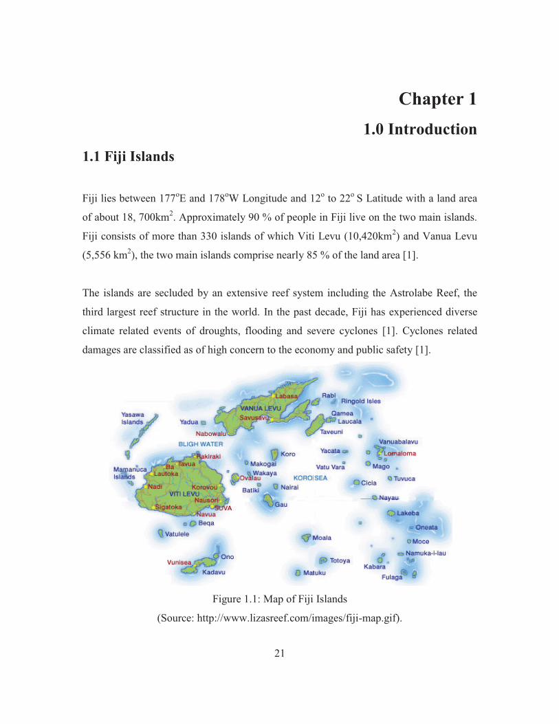
Fiji lies between 177oE and 178oW Longitude and 12o to 22o S Latitude with a land area
of about 18, 700km2. Approximately 90 % of people in Fiji live on the two main islands.
Fiji consists of more than 330 islands of which Viti Levu (10,420km2) and Vanua Levu
(5,556 km2), the two main islands comprise nearly 85 % of the land area [1].
The islands are secluded by an extensive reef system including the Astrolabe Reef, the
third largest reef structure in the world. In the past decade, Fiji has experienced diverse
climate related events of droughts, flooding and severe cyclones [1]. Cyclones related
damages are classified as of high concern to the economy and public safety [1].
Figure 1.1: Map of Fiji Islands
(Source: http://www.lizasreef.com/images/fiji-map.gif).
22
In order to involve private sector in renewable energy generation in rural areas the
government has a rural electrification policy and a charter for “Renewable Energy Based
Rural Electrification with Participation of Private Enterprise” to guide the Renewable
Energy Service Companies (RESCOs) for development of infrastructure and
accelerations of investment in rural areas. Furthermore, the government provides fiscal
incentives, accelerated depreciation of renewable assets, tax holiday and custom duty
exemption on imports and use renewable energy equipments [2].
1.2 Energy Situation in the Pacific
Threats to energy security, global warming and risk associated with climate change in
pacific island countries (PICs) have boosted the interest in sustainable, cleaner and
modern alternatives in energy generation [3]. The use of renewable resources in energy
generation increases long term energy security and provides a method of mitigating the
impact of climate change for the fragile economies in the PICs where a bulk of the
revenue is spent on importing fuel for energy generation [4].
In 2008, Marshall Islands electric utility had a major financial and economical crisis due
to increase in global fuel price on the government of Marshall Islands to declare a state of
national emergency and to bailout the exiting electric utility [5]. Countries like Kiribati
have faced oil shortages in the past, severely affecting their electricity generation.
The Asian Development Bank has listed PICs amongst the 10 economies most
susceptible to oil price volatility in the Asia-Pacific region [3]. PICs have the highest
petroleum fuel dependency than any region in the world where approximately 85% of
energy generations are based on petroleum fuel.
PICs have been known for their excellent solar resource, which increases slightly toward
the equator [3]. Studies in Tuvalu and Kiribati have shown that photovoltaic energy
generation is the least cost option for energy generation with low operational and
23
maintenance costs [6]. Tokelau has recently installed 1MW PV solar systems to generate
90% of their energy demand using solar energy. Tuvalu, Tonga, Fiji also have 40kW [7],
1,300kW and 57kW installed grid connected PV systems respectively. Grid connected
systems have also been implemented in FSM, Niue, Palau, Nauru and Marshall Islands
under the REP-5 Programme [8]. In addition, thousands of Solar Home Systems( SHS)
are operational in Tuvalu, Papa New-Guinea (PNG), Fiji, Solomon islands Kiribati and
Republic of Marshal Islands (RMI) to provide basic electrification to remote island
communities strengthening energy security and off-setting the use of fossil fuels.
Besides solar energy, other renewable energy sources are also being investigated for
their potential in the Pacific region. Wind based electricity generation systems are
installed in Cook Islands, Fiji, Vanuatu, New Caledonia and French Polynesia [9]. The
wind resource tends to decrease towards the equator and many of the islands with good
wind power potential lie in the paths of cyclones. These factors make wind energy
development more challenging.
Fiji, PNG, Solomon Islands, Samoa and Vanuatu have sufficient land area and hydro
resources to support hydropower generation. In Fiji, on average hydropower contributes
approximately 48% of all electricity generation while in French Polynesia, New
Caledonia, Samoa, the Solomon Islands and Vanuatu there are small hydro power plants
for provincial centres or villages [9]. The region along the ring of fire is always of
interest for geothermal energy generation. To date, only PNG has a 70 MW system on
east coast of Lihir Island. While, geothermal power development has been proposed for
Fiji and Vanuatu [10].
Although PICs are surrounded by large ocean areas, to date there are no installed ocean
energy systems. There are plans for a wave energy generation system in Kosrae
(Federated States of Micronesia) and feasibility studies for the exploitation of this
resource are been carried out in Tonga [3].
24
Biofuel production in the Pacific has been looked at as an option for replacement of
diesel in Combustion-Ignition (CI) engines. Coconut oil blends are used in Fiji and
Vanuatu as a replacement of diesel in motor vehicles and diesel generators. Currently,
Fiji and PNG have 9,300 kW and 300 kW system biomass based power plants which use
chip wood and bagasse to produce electricity [11-12].
In addition to exploitation of sustainable resources in energy generation to strengthen
energy security in the Pacific, energy efficiency (EE) programs have been also
implemented by many countries and the national energy policy plans in eleven PICs have
energy efficiency as a major focus [13].
1.3 Fiji’s Energy Situation
Electricity demand in Fiji has increased rapidly from 203 kWh in 1980 to 786 GWh in
2009, and with a projected increase of 7% at an annual growth rate of 0.23%, the
electricity demand is expected to be 1150 GWh in 2015 [7]. Converting to oil equivalent,
these figures range from 85.3 million litres in 1980 to 91.4 million litres in 2009 and is
expected to be 134 million litres in 2015. In terms of money, Fiji’s fuel imports have
increased 3 folds from $400 million in 2004 to 1.2 billion in 2008. Energy is the basic
ingredient for all household and industrial growth, thus an increase in the cost of
generation has adverse impact on individuals as well as operation of businesses in Fiji
[2].
In 2010, around 66.8% of electricity demand in Fiji is met by renewable sources
including 62.1% hydro, 4.1% biomass and 0.6% from wind and other renewable sources.
Preliminarily assessments by Fiji commerce commission show that Fiji is capable of
generating 54% of its total energy needs through renewable sources in the near future (no
including transport) [14].
25
Based on assessment of the primary data by commerce commission of Fiji in 2010, the
unit (per kWh) cost of electricity generation from diesel fuel and hydro system were 48
and 11.5 cents per kWh respectively. The transmission, distribution and retail (TDR)
costs of electricity were 13 cents per kWh, making the final unit costs for electricity
generation stands at 61 and 24.5 cents per kWh respectively [4]. Furthermore, at a 60/40
and 40/60 hydro/diesel ratio, the unit cost of electricity approximates to 39.1 and 46.4
cents respectively. The cost of electricity will be 40.78 and 59.91 cents per kWh with an
additional 25% return on equity for FEA. These Figures are subject to change in the near
future with increase in fuel price, inflation, natural disasters (drought) and increase in
demand. [4] Thus, Fiji needs to develop other alternative sources of energy to meet its
increasing demand and to stabilize the energy market from increasing fuel price
variability, inflation, natural disasters (drought/cyclones).
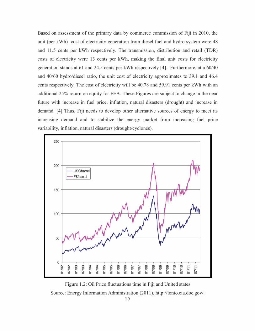
Figure 1.2: Oil Price fluctuations time in Fiji and United states
Source: Energy Information Administration (2011), http://tonto.eia.doe.gov/.
26
Fig 1.2 shows the variation in oil price for the period 2001-11. As discussed above, Fiji
and other pacific island countries generate most of their electricity from fossil fuel based
systems. The fuel price fluctuation has a significant impact on cost of electricity
generation and pose financial and energy security risk to Fiji and its pacific island
country partners which spend a significant amount of their revenue on purchase of fuel
[5].
1.4 Renewable Energy and Fiji Government
Energy generation and utilization in Fiji is governed by the energy act of Fiji. There are nine
energy acts in place to deal with supply, generation, use, exploitation, storage, carriage, price
control, transmission and distribution in Fiji. There is also an Environment Management Act
(EMA) that is based on the legislative framework for sustainable development of land and
water resource management for energy generation in Fiji [15].
To promote energy security, the Government of Fiji, through the Fiji Department of Energy
(FDoE) is encouraging the development and use of renewable energy sources such as
biomass, bio-fuels, hydro, solar, geothermal, tidal, wave and wind in transportation and
energy generation sector. FDoE is also promoting the use of energy efficient appliance and
transportation vehicles to reduce importation of petroleum products [16].
Imported fuel such as diesel, gasoline and benzene are the major source of energy in the
transportation and non-renewable electricity generation sector in Fiji. Rising energy demand
has a direct adverse effect on the cost of living, basic food items and services in Fiji [16].
According to the 2012 budget, factors that continue to affect the provision of energy
services in Fiji are: “… limited internal markets, lack of economies of scale, high
transportation costs, remoteness of islands, vulnerability to natural disasters, significant
difficulties in attracting foreign investments, and limited human and institutional capacity.”
[16].
27
In 2006, the government developed a National Energy Policy (NEP) to “reduce fuel imports,
strengthen energy security and build up a cost effective, resource efficient and
environmentally sustainable energy sector.” The NEP policy focuses on energy security,
national energy planning, renewable energy and power sector. The policy provides a structure
for all stakeholders to optimize the utilization of energy resources [16]. This policy is
currently being revised.
In 2012, FDoE allocated $FJD 2.7 million for Bio-Diesel fuel implementation Project. The
current projects in progress involve production of bio-fuel using copra and jatropha.
Furthermore, FDoE is also pursuing the production of ethanol form molasses in the near
future. Under its rural electrification programme, in 2012 FDoE with donor assistance
directed $4.0 million toward installation of 500 diesel generators, 1400 Solar Home Systems
and 3 mini hydro power plant in rural communities and schools around the country [16].
Currently, FDoE is developing an energy legislation that will regulate the production, supply
and use of energy. In addition, the legislation ensures to lessen the impacts of energy
production, supply and use on the environment [16].
1.5 FEA
Fiji Electricity Authority (FEA) is the only electricity utility in Fiji and serves over 147,
000 customers. FEA has a peak annual demand of over 138MW and supplies about
740GWh of energy per year. The grid network consists of 140km of 132kV transmission
lines and 8,300 km of medium & low voltage distribution lines, which are monitored by
Supervisory Control and Data Acquisition (SCADA) system as shown in Figure1.3 [15].
28
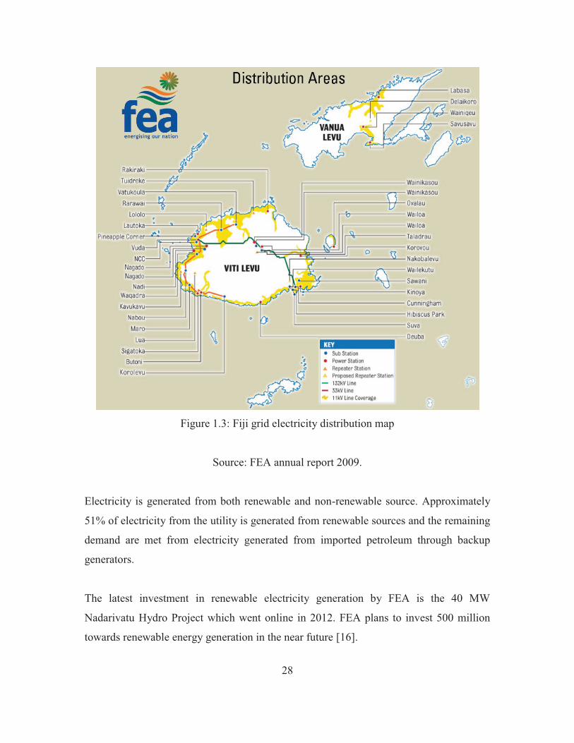
Figure 1.3: Fiji grid electricity distribution map
Source: FEA annual report 2009.
Electricity is generated from both renewable and non-renewable source. Approximately
51% of electricity from the utility is generated from renewable sources and the remaining
demand are met from electricity generated from imported petroleum through backup
generators.
The latest investment in renewable electricity generation by FEA is the 40 MW
Nadarivatu Hydro Project which went online in 2012. FEA plans to invest 500 million
towards renewable energy generation in the near future [16].

29
1.6 Motivation of this project
Energy is the basic prerequisite for economic and sustainable development of human
society, which is associated with fundamental aspects of economic growth, education and
social development [17]. Ever increasing world population together with rising living
standards have boosted the world energy demand significantly [14]. On the other hand,
more than 50% of pacific island countries (PICs) population lack basic access to
electricity [6].
Investment in renewable energy in Fiji will provide a sustainable path to energy security
and economic development. Cyclones, drought and flood are the three most common
weather hazards experienced in Fiji and have caused the country over 700 million dollars
in losses over the past 10 year [15]. These events also adversely affect the energy
security, for example reduced rainfall quickly increases the fossil fuel usage in electricity
production [18]. PV systems and other renewable energy technologies will help Fiji to
diversify its energy options greatly reduce the dependence on fossil fuel based energy
generation.
The unique geographical characteristics and sparsely populated islands separated by large
distances in Pacific island countries provide a challenge for extension of main grids and
rural electrification [6]. The FEA grid network in Fiji is small and is mostly limited to
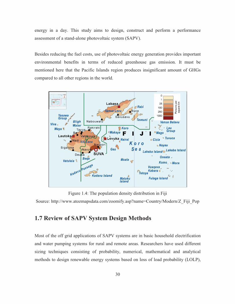
people in larger islands and close to the network. The FEA grid distribution (Fig 1.3) and
the population density map for Fiji (Fig 1.4) show that most of the inland areas in Fiji are
without electricity and grid extension to these is also not economically feasible.
Preliminary assessments by Fiji Department of Energy (FDoE) show that cost of
petroleum fuel in outer islands and inland areas is 10 to 40% higher than the fuel price in
central mainland areas. Stand-alone renewable energy based systems are economically
and technically attractive options for electricity generation in these areas. In Fiji, the
initial capital cost of a photovoltaic system is much lower than for most of the other
alternative renewable energy systems and on average Fiji receives 5 kWhm-2 of solar
30
energy in a day. This study aims to design, construct and perform a performance
assessment of a stand-alone photovoltaic system (SAPV).
Besides reducing the fuel costs, use of photovoltaic energy generation provides important
environmental benefits in terms of reduced greenhouse gas emission. It must be
mentioned here that the Pacific Islands region produces insignificant amount of GHGs
compared to all other regions in the world.
Figure 1.4: The population density distribution in Fiji
Source: http://www.atozmapsdata.com/zoomify.asp?name=Country/Modern/Z_Fiji_Pop
1.7 Review of SAPV System Design Methods
Most of the off grid applications of SAPV systems are in basic household electrification
and water pumping systems for rural and remote areas. Researchers have used different
sizing techniques consisting of probability, numerical, mathematical and analytical
methods to design renewable energy systems based on loss of load probability (LOLP),
31
energy balance, reliability of supply, optimization of energy output and life cycle cost
analysis [19-33].
Hybrid computational techniques combining two or more methods in sizing have been
used successfully [20, 26, 29-33] to achieve solutions to meet complex system
requirements. Sizing based on loss of load probability in combination with life cycle cost
optimization [21, 27], neural network [30], capacity & generation shortage [31], and
individual component simulation [32] techniques have been used to effectively size
SAPV systems. The choice of sizing and design techniques are dictated by the
complexity of input data, system purpose, the accuracy and reliability needed in the
simulating the energy output of the designed system. These techniques have been used to
size solar PV, wind and hybrid systems (solar-wind-hyrdo-diesel) among others.
Hontoria et al [30] presented a sizing approach based on neural network technique
utilizing Multilayer Perceptron (MLP) with LOLP and radiation data in designing SAPV
system for a hypothetical site in Spain. While, Lucio et al designed and assessed the
performance of PV system design using three probabilistic methods [31]. The first
method consisted of fixed number of battery backup and recharge while the second is
based on LOLP and the third is based on utilizing Markov Chain in modelling the PV
system.
Kaldellis et al [29] utilized energy balance technique to design SAPV systems including
variable system reliability for remote consumers in Greek territories. A detailed SAPV
system energy balance analysis was carried out on hourly bases using long term
measurements. Whilst, Posadillo et al [33] presented an analytical method based on
LOLP for sizing and evaluating SAPV systems with varying load demand and plane
inclination on hourly bases.
Chakrabarti et al [34] detailed the feasibility of SAPV system for remote islands from
environmental and socio-economic point of view. Notton et al [35] presented a detailed
32
evaluation of sensitivity on sizing methods using numerical methods and hourly load
profiles.
Kaushika et al [36] investigated a computational scheme for optimal sizing of SAPV
system with interconnected PV array and battery bank.
Cabral et al [31] presented a stochastic sizing methods for SAPV system based on loss of
power supply probability (LPSP) and performed simulation of PV system at individual
input parameter level consisting of solar radiation, photovoltaic array, energy storage,
loss of load calculation and component sizing based on economical and reliability
aspects. Another study by Cabral et al [32] also entails simulation and actual component
performance.
1.8 Review of SAPV System Performance studies
An essential part of performance evaluation is to understand the energy loss in PV system
and develop methods to minimize these losses and provide recommendations for
improvements in future system design. Energy losses in PV system can be detected by
monitoring and analyzing performance data [37]. Performance monitoring has been used
in the past to develop guides for PV performance [38] and to provide data for future
installation of PV system. Reliable SAPV performance knowledge under field conditions
is essential in selecting, designing and predicting SAPV system reliability and energy
output from a wide combination of SAPV systems and components [39] [40].
Chel et al [41] presented a 2.32kWp SAPV system performance consisting of PV array,
battery and inverter for four weather conditions in India. The performance of SAPV
system shows that the daily SAPV system efficiency range from 3.2% to 5.9%. Whilst,
Tripathy et al [42] evaluated the performance of 20 kWp PV system for a sports school in
India consisting of 4 subarray and found that the overall conversion efficiency of PV
system is 3.48%.
33
Sasitharanuwat et al [40] evaluated the performance of 10kWp PV system for a isolated
building in Thailand consisting of three subarrays of 3.672 kW p of amorphous thin film,
3.6 kWp of polycrystalline silicon and 2.88 kWp of hybrid a-Si solar cells. The efficiency
of the respective arrays were found to be 6.26%, 10.48 and 13.78%.
Pratt R.G [43] presented a two year performance evaluation of 4kW amorphous-silicon
photovoltaic system in Michigan on the durability and reliability of PV system
performance on seasonal bases. Whilst, Jumie Yuventi [44] presented a method for
evaluating the influence of wiring in photovoltaic system design on the performance of
SAPV components. The paper illustrates the use of the outline method to show the
influence of wiring on the direct current operating voltage needed to achieve maximum
power performance for the system.
Muñoz et al [45] evaluated the performance of SAPV system without maximum power
point tracker. (MPPT) for Mediterranean climate and concluded that SAPV systems
without MPPT have lower efficiencies than systems with MPPT and suggested
consideration of such system in regions with high solar irradiances.
Sadok et al [46] studied the performance and the representative parameters that influence
the performance of SAPV system in south Algeria. While, Rehman et al [47] carried out
performance evaluation analysis of 5.28kW SAPV system in Saudi Arabia and found that
PV array efficiency varies from 4.1% to 11.9%. Shrama et al [39] investigated the
technical performance of SAPV array under field condition in New Delhi for two
individual 1.2 kWp and 1.12kWp subarrays on daily, monthly and annual basis. The result
shows that PV array efficiency varies from 3.9% to 9.5%.
The main objective of this study was to design and construct an optimum SAPV system
based on both LOLP and reliability of supply and generate PV system components
performance data for this part of the world under field operating conditions that assist in
prediction of electricity prediction from similar SAPV and even larger PV systems
installed in the future.
34
Chapter 2 2.0 Background
2.1 Sun
Sun is the ultimate source of energy and plays a important role in a wide spectrum of
physical and biological process which drives the earth’s energy circulation. The total
power output of the sun is approximately 3.8 x1026 W. Energy in the sun results from the
fusion of hydrogen atom in the solar interiors of four hydrogen nuclei having masses
nearly 1% larger than the helium nucleus. The Hydrogen nuclei fuse to form helium and
the mass deficit results into energy. The energy resulting from fusion are emitted in the
form of electromagnetic radiation.
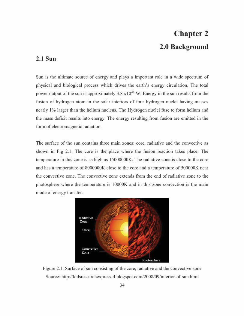
The surface of the sun contains three main zones: core, radiative and the convective as
shown in Fig 2.1. The core is the place where the fusion reaction takes place. The
temperature in this zone is as high as 15000000K. The radiative zone is close to the core
and has a temperature of 8000000K close to the core and a temperature of 500000K near
the convective zone. The convective zone extends from the end of radiative zone to the
photosphere where the temperature is 10000K and in this zone convection is the main
mode of energy transfer.
Figure 2.1: Surface of sun consisting of the core, radiative and the convective zone
Source: http://kidsresearchexpress-4.blogspot.com/2008/09/interior-of-sun.html
35
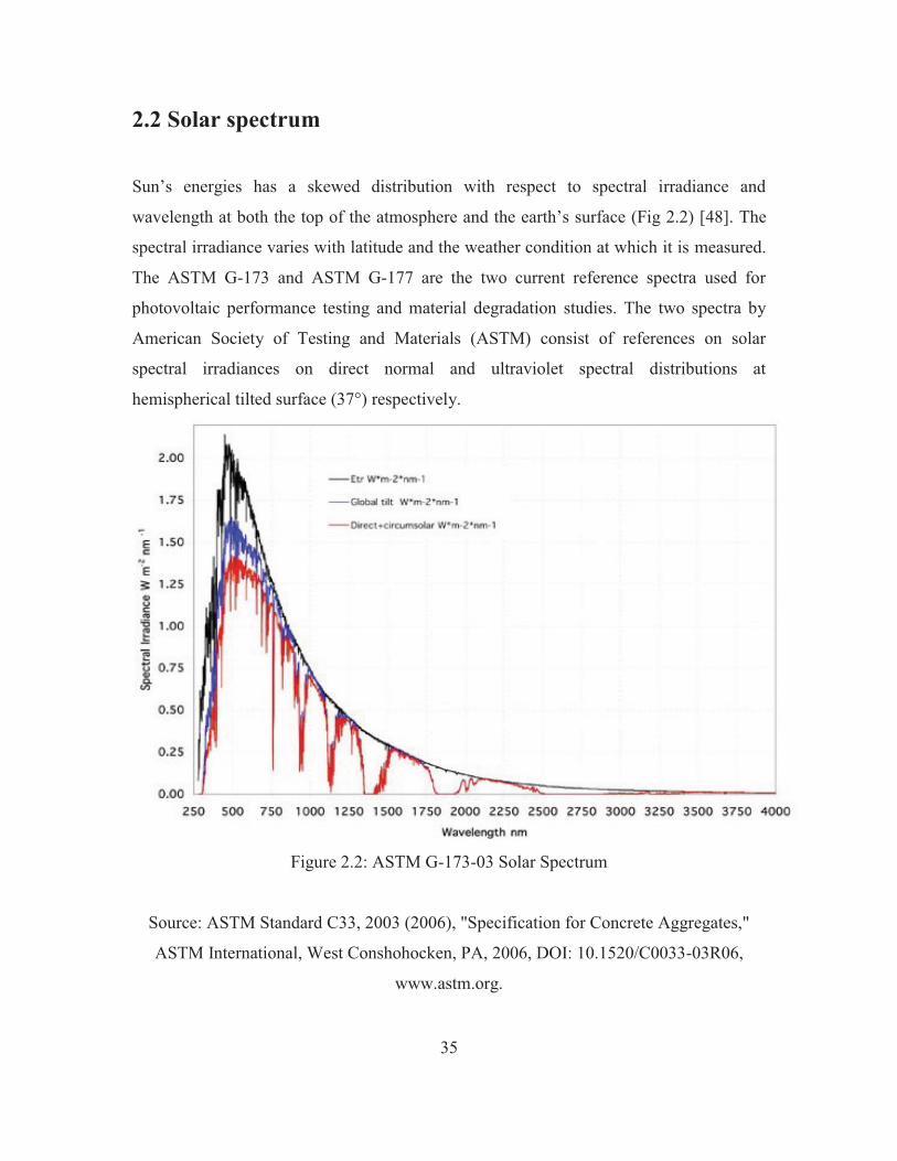
2.2 Solar spectrum
Sun’s energies has a skewed distribution with respect to spectral irradiance and
wavelength at both the top of the atmosphere and the earth’s surface (Fig 2.2) [48]. The
spectral irradiance varies with latitude and the weather condition at which it is measured.
The ASTM G-173 and ASTM G-177 are the two current reference spectra used for
photovoltaic performance testing and material degradation studies. The two spectra by
American Society of Testing and Materials (ASTM) consist of references on solar
spectral irradiances on direct normal and ultraviolet spectral distributions at
hemispherical tilted surface (37°) respectively.
Figure 2.2: ASTM G-173-03 Solar Spectrum
Source: ASTM Standard C33, 2003 (2006), "Specification for Concrete Aggregates,"
ASTM International, West Conshohocken, PA, 2006, DOI: 10.1520/C0033-03R06,
www.astm.org.
36
The current standard reference for terrestrial solar spectra in photovoltaic testing is
ASTM G-173-03. The solar spectra used in ASTM G-173 consist of G159 and ISO9845-
1 standards, which have now been superseded by ASTM G-173-03 for PV performance
evaluation [48]. The ASTM G-173-03 represents spectral terrestrial solar irradiance on
direct normal and hemispherical surface tilted at 37° at specified atmospheric conditions.
The specified atmospheric conditions are:
a) Absolute Air Mass of 1.5
b) Total column ozone content of 0.34 cm
c) Total integrated column water vapor content of 1.42 cm
d) Angstrom turbidity of 0.084 at 500 nm
e) Pressure, temperature, air density, aerosol density and molecular species density
as specified in 33 layers and documented in U.S. Standard Atmosphere [49].
f) Surface spectral reflectivity of light Soil as documented in ASTER Spectral
Reflectance Database [50].
2.3 PV module technology
Over the last 20 years, solar photovoltaic (PV) technology has evolved into a mature,
sustainable and adaptive technology. This technology is continually improving as solar
cells efficiencies increase by the use of materials that absorbing energies of all
frequencies in the solar energy spectrum and convert them into electrical energy. Bulk
manufacturing and increased raw material supply has edged photovoltaic power
generation in becoming a cost-effective alternative to conventional energy sources [51].
PV technology is divided in a number of distinct categories based on manufacturing
technology, active layer material, glazing materials, electrical connections and the energy

37
band gap of the materials. Over 80% of the photovoltaic industry is based on crystalline
silicon cells [52]. Mono-crystalline and the polycrystalline silicon solar cells are the two
major categories of crystalline solar cells. The monocrystalline solar cells have high
efficiency than the polycrystalline cells. However, low cost production of polycrystalline
solar cell has edged them to secure more of the installed photovoltaic market share based
on cost per watt.
The amorphous thin film, ribbon, boule and the microcrystalline cells are amongst the
other types of silicon based solar cells that have been projected to decrease the cost of
solar cells in the near future [53]. The low cost deposition techniques and approximately
1um thickness have paved the way for producing thin film solar cells modules at very
low cost. Other main thin film solar cell types consist of C(IG)S/CdS and CdTe/Cds cells.
To date, the highest solar cell efficiencies have been demonstrated by the group III-IV
solar cells. To increase cell and module efficiency by capturing most of the energy form
the broad solar electromagnetic spectrum multijunction solar cells consisting of GaAs,
InP and (TiO2, ZnO, Fe2O3, ZrO2, Nb2O5, Al2O3, and CeO2) are used [54]. Multijunction
solar cells consisting of GaAs, InP and the alloys has shown to increases the efficiency of
the cells with their high light absorption coefficient. The high stability against light
induced degradation and reduced weight of modules has ensured such modules to be
utilized in the satellite and space navigation applications [55].
The Hybrid heterojunction with Intrinsic Thin layer (HIT) solar cell is a combination of
crystalline and thin film solar cells. HIT solar cell and the quantum dot cells have a low
band gap semiconductor material incorporated into the cells to absorbed light of low
energy. HIT consists of an N-doped mono-crystalline layer sandwiched between the
intrinsic amorphous layer. The intermediate intrinsic thin layer forms a contact on both
sides of the mono-crystalline wafer. The P-doped a-Si layer is deposited on the front side
to form a P-N junction with the N-doped mono-crystalline wafer. To prevent free charge
carriers recombining on the back electrode the back contact amorphous layer are formed
with a highly N-doped wafer. HIT performance is highly stable against high temperatures
and light degradation than ordinary silicon solar cells. This method of hosting a small

38
bandgap material into a high band gap photovoltaic cell increases the current output
while retaining a large portion of the high voltage output characteristics.
The search of low cost active layer with low energy input has smoothened the path for
organic solar cell in becoming a key player in the photovoltaic industry. Research in the
area of organic solar cell has advanced the organic cell technology into a prospective
member of photovoltaic industry. Organic solar cell research is headed with two major
approaches, the first approach deals with the full organic approach of solar cells while the
second approach consists of the hybrid approach in which the cells retain part of the
organic material together with part of organic components to make a PV cell [56].
2.4 Operation of PV modules P-N junction
Most of the solar cells are made up of silicon and have a P-N junction to separate charge
carries, thus it is better to understand the operation of P-N junction in PV cell. The basic
working principles of all PV cells are essentially based on the photovoltaic effect. The
main processes of photovoltaic effect are a) generation of the charge carriers at the
junction on absorption of photons. b) separation of the charge carriers at the junction and
(c) collection of charge carriers at the ends of the junction. In general, photon induced
electron- hole pairs generated near the P-N junction are easily separated without much
recombination.
P-N junction is made up of two different types of semiconductor (N-type and P type). A
N-type semiconductor layer consist of a high concentration of free electrons which is
compensated by positively charged donor atoms whilst, P-type semiconductor layer has a
high concentration of holes as the major charge carrier and is compensated by negatively
charged acceptor atoms as shown in Fig 2.3.

39
Figure 2.3: Schematic representation of N-type and P-type semiconductor
A N-type material has a high affinity to electrons and allows electrons to diffuse through
the junction towards N-type material. Whilst, the P-type layer has high affinity to holes
thus allows holes to diffuse through the junction into the P-type semiconductor. To
minimize recombination near the junction a high bandgap semiconductor is chosen to
develop a energy barrier between either side of P-N junction is formed as shown in Fig
2.5.
Upon contact the free charge carriers from N-type (electrons) and P-type (holes)
semiconductor diffuse at the junction. At the contact point the electrons and holes
recombine to form a charge depleted region. The recombination of charge carriers at the
junction sets up a electric field between the two sides of the layer which averts any
further migration of charge carriers from each layer At equilibrium. The P-N junction has
a schematic as shown in Fig 2.4 and an energy profile as shown in 2.5. Charge carries are
generated upon photons strike at the solar cell. In general electron hole pairs generated
near the depleted region are easily separated without much recombination due to the
induced electric field between the N and P type materials.
40
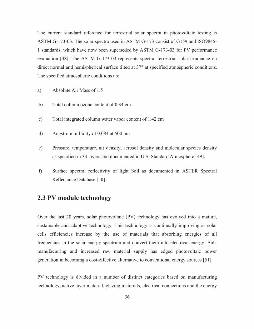
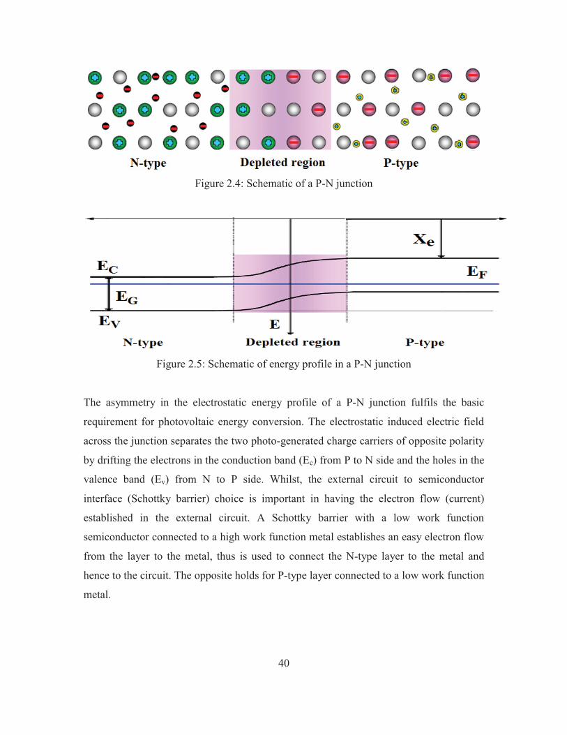
Figure 2.4: Schematic of a P-N junction
Figure 2.5: Schematic of energy profile in a P-N junction
The asymmetry in the electrostatic energy profile of a P-N junction fulfils the basic
requirement for photovoltaic energy conversion. The electrostatic induced electric field
across the junction separates the two photo-generated charge carriers of opposite polarity
by drifting the electrons in the conduction band (Ec) from P to N side and the holes in the
valence band (Ev) from N to P side. Whilst, the external circuit to semiconductor
interface (Schottky barrier) choice is important in having the electron flow (current)
established in the external circuit. A Schottky barrier with a low work function
semiconductor connected to a high work function metal establishes an easy electron flow
from the layer to the metal, thus is used to connect the N-type layer to the metal and
hence to the circuit. The opposite holds for P-type layer connected to a low work function
metal.
41
2.5 Efficiency
Photovoltaic (PV) effect was first discovered in 1839 by Alexandre-Edmond Becquerel
and in 1883 Charles Fritts introduced the 1% efficient solar cell [57]. To date most of the
PV cells are made up of either direct or a indirect bandgap semiconductors.
Shockley and Queisser did the seminal calculation on the limit of PV efficiency in 1961
and many researchers have extensively studied factors that reduce PV cell performance
and the way to mitigate the fundamental physical limit in Shockley and Queisser
calculation [58]. The Shockley and Queisser assumption on the efficiency of PV modules
is based on the fundamentals of blackbody radiation, recombination and spectral loss
within a PV cell. The peak theoretical efficiency of single junction PV cell has been
found to be 33.7% whilst for multi-junction and concentrated PV cells the Shockley and
Queisser theoretical limit has been determined to be 68 and 86% respectively. [59] Newer
methods of increasing the efficiency comes from concentrating solar radiation, hot
electron capture, down conversion of solar radiation to a common frequency, infrared
capture and lowering reflective with honeycomb surface texture.
To-date the highest efficient (43.5%) PV cell is a multi-junction concentrated
photovoltaic cell (CPV) developed by Solar Junction [60]. Crystalline silicon and thin
film cell technologies have emerged a long way since its first introduction and have
achieved 27.6% and 20.3% efficiency in 2012 respectively. Dye sensitized (DSSC) and
quantum dot cells are the emerging types of PV cell and have achieved efficiencies of
10% or more while Quantum dot cell have a highest recorded efficiency of 5.1%. Fig 2.6
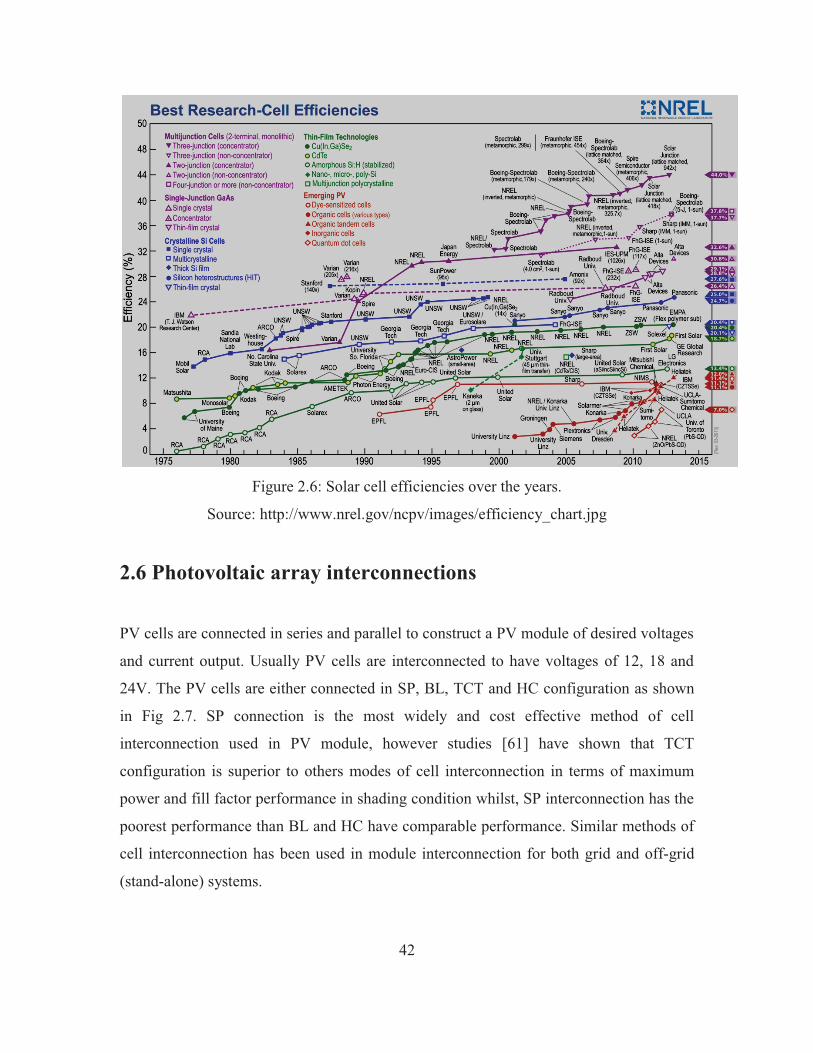
shows the highest archived solar cell efficiency as of 2012.
42
Figure 2.6: Solar cell efficiencies over the years.
Source: http://www.nrel.gov/ncpv/images/efficiency_chart.jpg
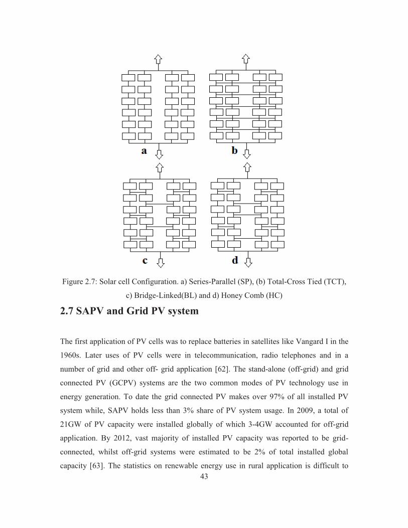
2.6 Photovoltaic array interconnections
PV cells are connected in series and parallel to construct a PV module of desired voltages
and current output. Usually PV cells are interconnected to have voltages of 12, 18 and
24V. The PV cells are either connected in SP, BL, TCT and HC configuration as shown
in Fig 2.7. SP connection is the most widely and cost effective method of cell
interconnection used in PV module, however studies [61] have shown that TCT
configuration is superior to others modes of cell interconnection in terms of maximum
power and fill factor performance in shading condition whilst, SP interconnection has the
poorest performance than BL and HC have comparable performance. Similar methods of
cell interconnection has been used in module interconnection for both grid and off-grid
(stand-alone) systems.
43
Figure 2.7: Solar cell Configuration. a) Series-Parallel (SP), (b) Total-Cross Tied (TCT),
c) Bridge-Linked(BL) and d) Honey Comb (HC)
2.7 SAPV and Grid PV system
The first application of PV cells was to replace batteries in satellites like Vangard I in the
1960s. Later uses of PV cells were in telecommunication, radio telephones and in a
number of grid and other off- grid application [62]. The stand-alone (off-grid) and grid
connected PV (GCPV) systems are the two common modes of PV technology use in
energy generation. To date the grid connected PV makes over 97% of all installed PV
system while, SAPV holds less than 3% share of PV system usage. In 2009, a total of
21GW of PV capacity were installed globally of which 3-4GW accounted for off-grid
application. By 2012, vast majority of installed PV capacity was reported to be grid-
connected, whilst off-grid systems were estimated to be 2% of total installed global
capacity [63]. The statistics on renewable energy use in rural application is difficult to
44
detail in developing countries due to installation data not collected systematically by any
international organization in these countries [64].
For majority of remote and isolated users, off-grid PV electricity is less expensive than
extending the power grid. Off grid and mini grid application of PV systems provides
modern energy access to billions of people in Africa, China, India and Latin America for
lighting and communication needs [64]. The incentive driven approach of PV system
with high feed in tariffs has boosted the use of PV in grid connected system over the off-
grid systems [63]. Grid connected PV system mainly consists of large solar farms and
roof top systems connected to the grid via a two-way meter (net-metering).
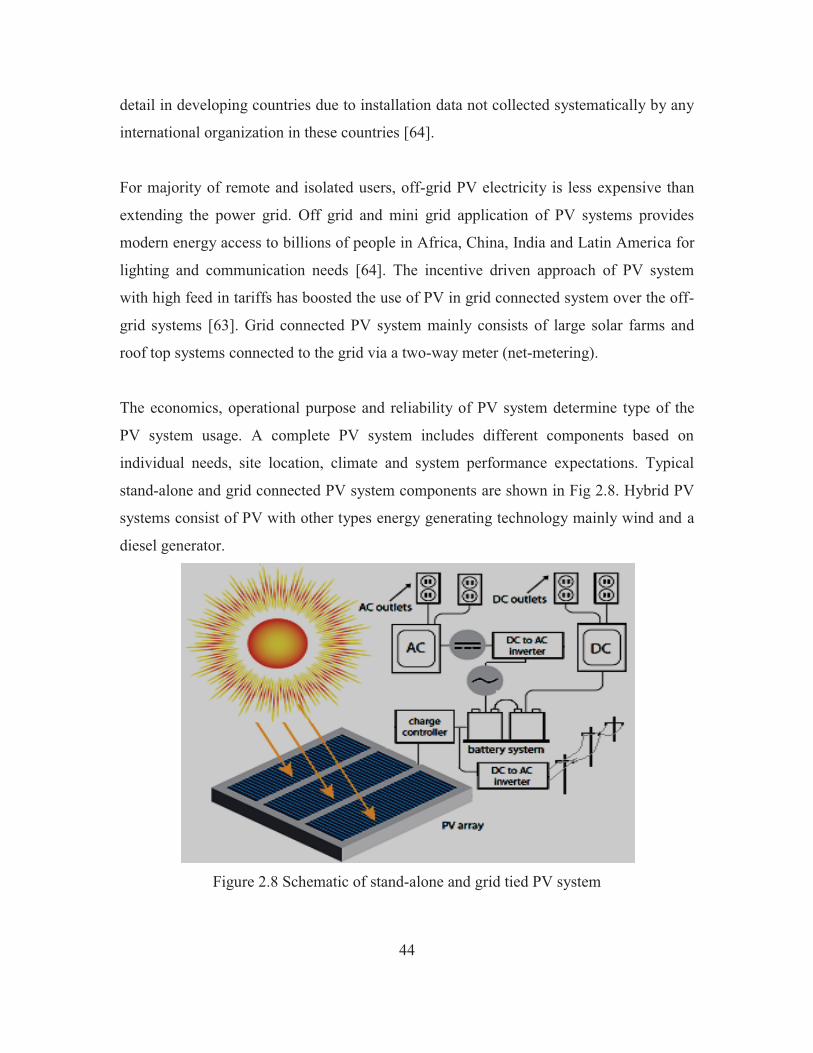
The economics, operational purpose and reliability of PV system determine type of the
PV system usage. A complete PV system includes different components based on
individual needs, site location, climate and system performance expectations. Typical
stand-alone and grid connected PV system components are shown in Fig 2.8. Hybrid PV
systems consist of PV with other types energy generating technology mainly wind and a
diesel generator.
Figure 2.8 Schematic of stand-alone and grid tied PV system
45
The operating behaviour of stand-alone systems is more complex compared to grid-
connected PV systems. A critical aspect of PV system design is sizing. In PV systems,
incorrect sizing may result in systems being incapable of functioning, faster component
ageing or total system failure. It is important to determine the optimal balance of PV
system components taking into consideration the local climate and reliability of desired
system. A critical factor that must be considered in PV system design is the optimisation of the
technologies and system economics [65]. With the ever changing world of technology and
PV system components, the optimal balance of system components is a important factor
in achieving a minimum cost of energy. With a wide spread of PV system component and
technology, use of software tools are highly valuable in computing and simulating
optimal PV system based on minimizing cost and optimizing reliability [66].
The software tools are either empirical or numerically based on individual components
that make up the balance of system (BOS). The usefulness and accuracy of various tools
have been extensively studied [67] taking into account the electrical, thermal, solar
spectral, optical effects and system configuration of PV system [68-69].
Various models have been successively incorporated into software programs to perform
complex hourly calculations and also forecast viability of system on short and long term
economic situation. Regardless of the complexity involved in sizing PV system software
with a large number of components and combinations of balance of system, sizing tools
has in the past shown high levels of accuracy in evaluating performance of PV system.
[70]
2.8 Photovoltaic market status
Photovoltaic energy conversion is considered as one of the most promising renewable
energy technology amongst all other renewable energy technologies [71]. It has the
potential to mitigate greenhouse gas emissions and contribute significantly to a clean
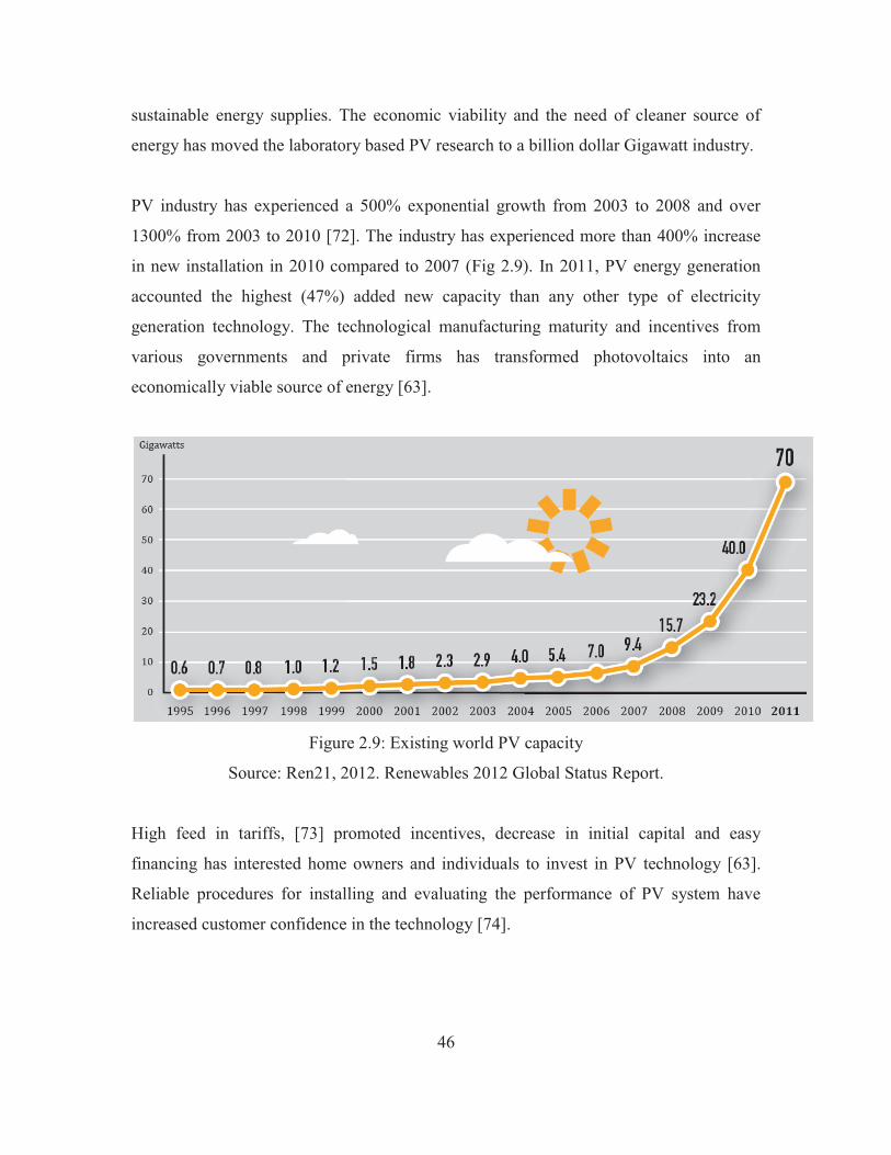
46
sustainable energy supplies. The economic viability and the need of cleaner source of
energy has moved the laboratory based PV research to a billion dollar Gigawatt industry.
PV industry has experienced a 500% exponential growth from 2003 to 2008 and over
1300% from 2003 to 2010 [72]. The industry has experienced more than 400% increase
in new installation in 2010 compared to 2007 (Fig 2.9). In 2011, PV energy generation
accounted the highest (47%) added new capacity than any other type of electricity
generation technology. The technological manufacturing maturity and incentives from
various governments and private firms has transformed photovoltaics into an
economically viable source of energy [63].
Figure 2.9: Existing world PV capacity
Source: Ren21, 2012. Renewables 2012 Global Status Report.
High feed in tariffs, [73] promoted incentives, decrease in initial capital and easy
financing has interested home owners and individuals to invest in PV technology [63].
Reliable procedures for installing and evaluating the performance of PV system have
increased customer confidence in the technology [74].
47
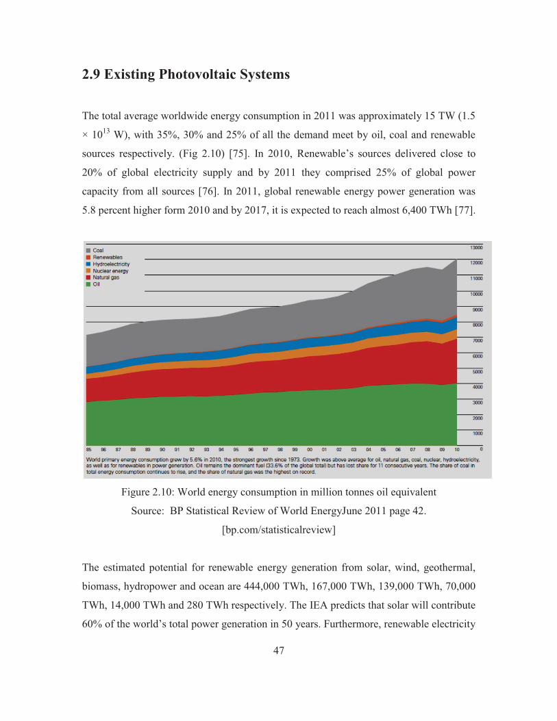
2.9 Existing Photovoltaic Systems
The total average worldwide energy consumption in 2011 was approximately 15 TW (1.5
× 1013 W), with 35%, 30% and 25% of all the demand meet by oil, coal and renewable
sources respectively. (Fig 2.10) [75]. In 2010, Renewable’s sources delivered close to
20% of global electricity supply and by 2011 they comprised 25% of global power
capacity from all sources [76]. In 2011, global renewable energy power generation was
5.8 percent higher form 2010 and by 2017, it is expected to reach almost 6,400 TWh [77].
Figure 2.10: World energy consumption in million tonnes oil equivalent
Source: BP Statistical Review of World EnergyJune 2011 page 42.
[bp.com/statisticalreview]
The estimated potential for renewable energy generation from solar, wind, geothermal,
biomass, hydropower and ocean are 444,000 TWh, 167,000 TWh, 139,000 TWh, 70,000
TWh, 14,000 TWh and 280 TWh respectively. The IEA predicts that solar will contribute
60% of the world’s total power generation in 50 years. Furthermore, renewable electricity
48
generation is expected to expand by 1,840 TWh between 2011 and 2017, this is an
increase of almost 60 percent from the period 2005 to 2011 [77].
The IEA predicts that 710 GW of PV systems will be installed by 2017. China is
expected to account for the biggest share of 270 GW of new capacity, followed by U.S.
India, Germany and, Brazil with 56 GW, 39 GW, 32 GW and 32 GW respectively [77].
Solar photovoltaic power generation technology is the fastest growing energy generating
technology in the world. The major utilization of PV is in the energy sector, between
2006 and 2011 the global cumulative PV installation has increased by 10 folds, lifting the
total installed PV capacity from 7.0 GW to 70GW compromising of mostly grid
connected system [78]. In 2011, PV energy generation reported the highest (47%) new
capacity addition than any other type of electricity generation technology. The price of
PV module fell by more than 40% due to economics of mass production, competition
among manufacturers, technological advancement and a large drop of silicon price in
2011 has boosted the use of PV in energy generation around the world.
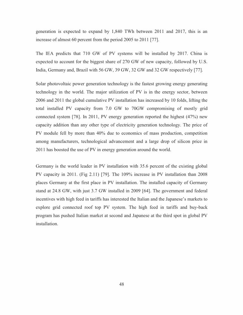
Germany is the world leader in PV installation with 35.6 percent of the existing global
PV capacity in 2011. (Fig 2.11) [79]. The 109% increase in PV installation than 2008
places Germany at the first place in PV installation. The installed capacity of Germany
stand at 24.8 GW, with just 3.7 GW installed in 2009 [64]. The government and federal
incentives with high feed in tariffs has interested the Italian and the Japanese’s markets to
explore grid connected roof top PV system. The high feed in tariffs and buy-back
program has pushed Italian market at second and Japanese at the third spot in global PV
installation.
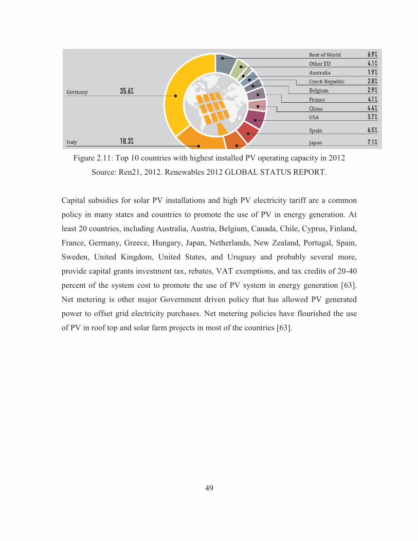
49
Figure 2.11: Top 10 countries with highest installed PV operating capacity in 2012
Source: Ren21, 2012. Renewables 2012 GLOBAL STATUS REPORT.
Capital subsidies for solar PV installations and high PV electricity tariff are a common
policy in many states and countries to promote the use of PV in energy generation. At
least 20 countries, including Australia, Austria, Belgium, Canada, Chile, Cyprus, Finland,
France, Germany, Greece, Hungary, Japan, Netherlands, New Zealand, Portugal, Spain,
Sweden, United Kingdom, United States, and Uruguay and probably several more,
provide capital grants investment tax, rebates, VAT exemptions, and tax credits of 20-40
percent of the system cost to promote the use of PV system in energy generation [63].
Net metering is other major Government driven policy that has allowed PV generated
power to offset grid electricity purchases. Net metering policies have flourished the use
of PV in roof top and solar farm projects in most of the countries [63].
50
Chapter 3
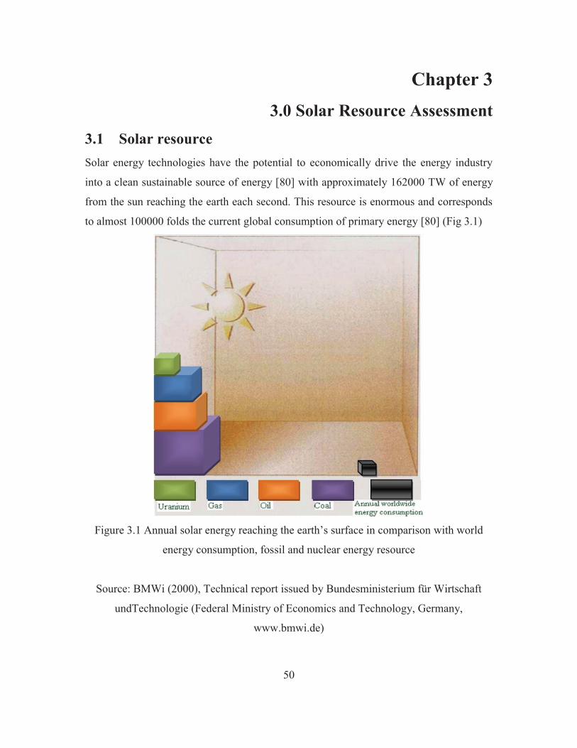
3.0 Solar Resource Assessment 3.1 Solar resource Solar energy technologies have the potential to economically drive the energy industry
into a clean sustainable source of energy [80] with approximately 162000 TW of energy
from the sun reaching the earth each second. This resource is enormous and corresponds
to almost 100000 folds the current global consumption of primary energy [80] (Fig 3.1)
Figure 3.1 Annual solar energy reaching the earth’s surface in comparison with world
energy consumption, fossil and nuclear energy resource
Source: BMWi (2000), Technical report issued by Bundesministerium für Wirtschaft
undTechnologie (Federal Ministry of Economics and Technology, Germany,
www.bmwi.de)
51
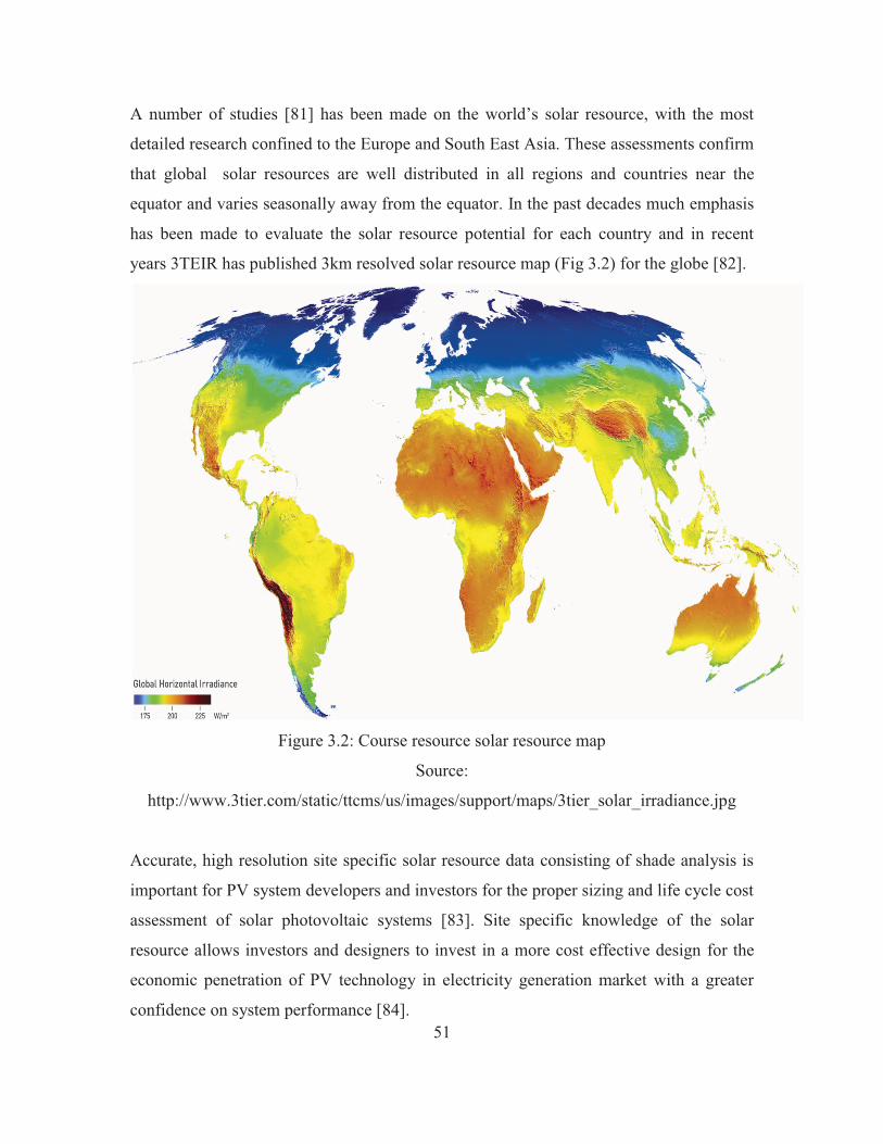
A number of studies [81] has been made on the world’s solar resource, with the most
detailed research confined to the Europe and South East Asia. These assessments confirm
that global solar resources are well distributed in all regions and countries near the
equator and varies seasonally away from the equator. In the past decades much emphasis
has been made to evaluate the solar resource potential for each country and in recent
years 3TEIR has published 3km resolved solar resource map (Fig 3.2) for the globe [82].
Figure 3.2: Course resource solar resource map
Source:
http://www.3tier.com/static/ttcms/us/images/support/maps/3tier_solar_irradiance.jpg
Accurate, high resolution site specific solar resource data consisting of shade analysis is
important for PV system developers and investors for the proper sizing and life cycle cost
assessment of solar photovoltaic systems [83]. Site specific knowledge of the solar
resource allows investors and designers to invest in a more cost effective design for the
economic penetration of PV technology in electricity generation market with a greater
confidence on system performance [84].
52
Satellite derived data and ground based measurement are two basic methods of solar
resource assessment. A satellite with GIS provides a swift, spatially resolved and low
cost method of solar resource assessment whilst, it has a disadvantage of low accuracy
and time resolution of assessment. On the other hand, ground based solar resource (direct
and diffuse) data measurements provides higher accurate and time resolved data, but at a
higher instrumentation cost.
Solar resource is greatly hindered due to shading caused by obstacles at the site. Thus,
shade analysis is essential component in determining the proper solar resource and the
performance of SAPV system at a site of installation.
3.2 Solar radiation variability
The variability of solar radiation is dependent on short term and long term climate over a
region. The day to day variation of solar radiation in the south pacific is dependent on the
daily synoptic weather conditions which is largely dependent on the general circulation of
winds and moisture resulting from the seasonal variation in diurnal heating and nocturnal
cooling of the land and sea surface [85]. The imbalance heating of atmosphere onsets a
gravity wave circulation in the lower atmosphere. In the pacific Madden–Julian
oscillation (MJO), gravity wave, monsoon onset and break periods and the position of the
South Pacific Convergence Zone (SPCZ) determines the daily, monthly and seasonal
variation of solar radiation [86]. The long-term variability of radiation is a result of yearly
variation of weather and climate in the three ocean basins (Indian, pacific, and Atlantic)
[87]. Even though the weather disturbance is thousands of kilometers away from a
region, the resulting disturbance wave travels a large distance and has significant impact
on the solar exposure and weather at these regions. The Southern Oscillation Index (SOI),
El’Nino Southern Oscillation (ENSO) and Indian Ocean Dipole (IOD) are the three most
used parameters used to study the variation of solar radiation at a region over a period of
year or more [88].
53
The ENSO is the largest driver of solar radiation in Fiji where a strong ENSO period
indicates higher solar radiation than normal [89]. SOI results from the zonal variation of
radiation and sea surface temperatures in the pacific ocean. A high SOI (greater than 0.8)
is a result of stronger Walker circulation which pushes the SPCZ over the south west of
Fiji islands which results in high solar radiation over the Fiji Islands [90]. However a
weak SOI (less than -0.8) results in a weaker trade winds and increased cloudiness over
the tropical pacific which in-turn results in low solar radiation. Based on the 10 years of
observation on ENSO in Fiji, the La Nina period event is associated with wet weather and
less solar radiation, while the El Nino is associated with dry seasons and high amounts of
solar radiation. However, there is a lag of 3 to 6 months between the two periods.
A positive IOD results when the western basin of the Indian ocean is warmer than the
eastern basin, this results in suppressed monsoon and high solar radiation in the pacific
[91]. A negative IOD results when the eastern basin of the Indian ocean is warmer than
the western basin, which results in enhanced monsoon and high cloud cover in the Pacific
(less solar radiation in Pacific). The most persistent long term variation of radiation is
known as the solar cycle and varies over a 11 year period [92].
3.3 Solar resource assessment
The measurement of radiation through satellite remote sensing, particularly solar
radiation provides an important method for determining the energy budget of the earth.
However due to the coarse resolution of satellite derived data, their use in comprehensive
analysis on the feasibility of energy generation at a site has become of a low significance.
To date there have been different methods used to assess the solar resource at a point of
interest [93-97]. Amongst the most common methods outlined in [93-97] are the physical,
analytical, numerical, statistical and empirical methods.
54
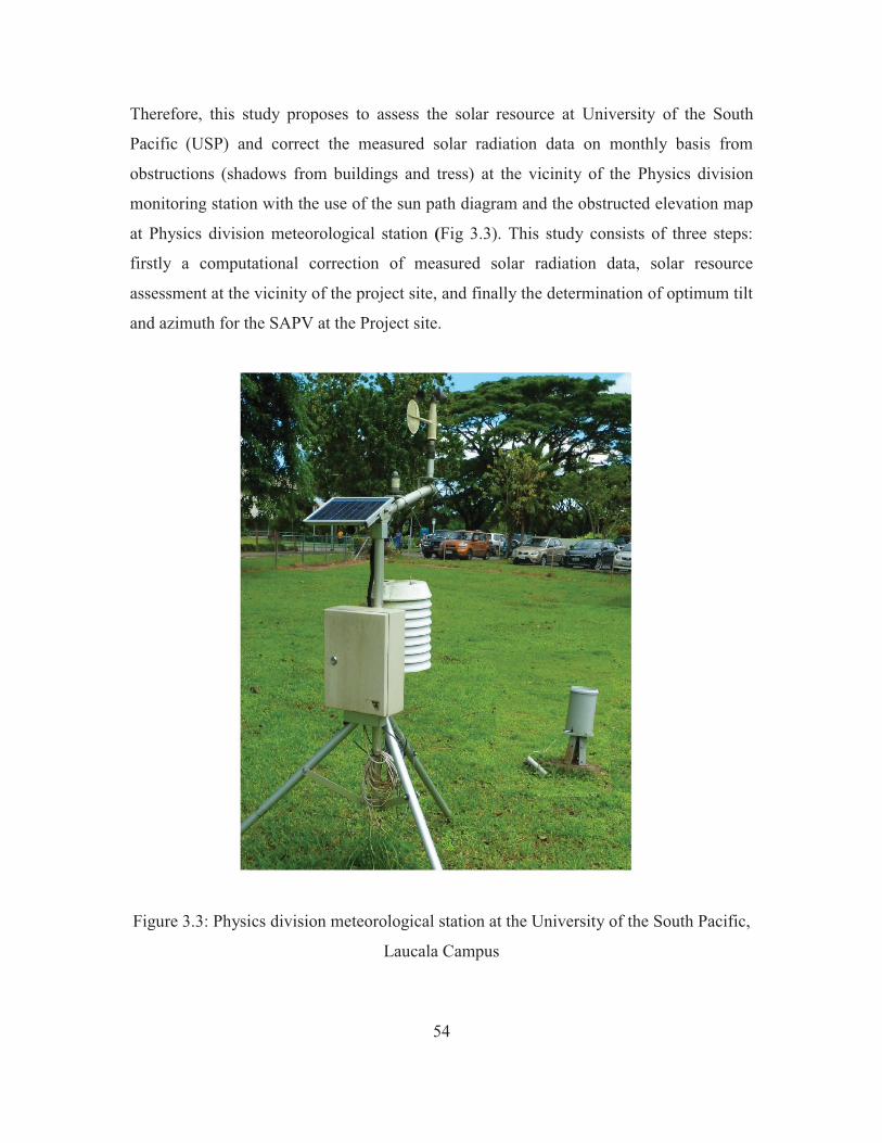
Therefore, this study proposes to assess the solar resource at University of the South
Pacific (USP) and correct the measured solar radiation data on monthly basis from
obstructions (shadows from buildings and tress) at the vicinity of the Physics division
monitoring station with the use of the sun path diagram and the obstructed elevation map
at Physics division meteorological station (Fig 3.3). This study consists of three steps:
firstly a computational correction of measured solar radiation data, solar resource
assessment at the vicinity of the project site, and finally the determination of optimum tilt
and azimuth for the SAPV at the Project site.
Figure 3.3: Physics division meteorological station at the University of the South Pacific,
Laucala Campus
55
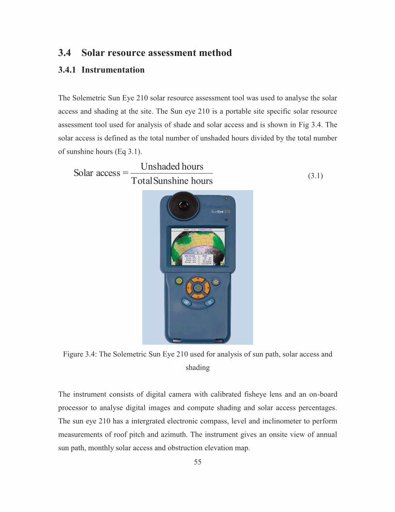
3.4 Solar resource assessment method 3.4.1 Instrumentation
The Solemetric Sun Eye 210 solar resource assessment tool was used to analyse the solar
access and shading at the site. The Sun eye 210 is a portable site specific solar resource
assessment tool used for analysis of shade and solar access and is shown in Fig 3.4. The
solar access is defined as the total number of unshaded hours divided by the total number
of sunshine hours (Eq 3.1).
hours Sunshine Totalhours Unshaded = accessSolar (3.1)
Figure 3.4: The Solemetric Sun Eye 210 used for analysis of sun path, solar access and
shading
The instrument consists of digital camera with calibrated fisheye lens and an on-board
processor to analyse digital images and compute shading and solar access percentages.
The sun eye 210 has a intergrated electronic compass, level and inclinometer to perform
measurements of roof pitch and azimuth. The instrument gives an onsite view of annual
sun path, monthly solar access and obstruction elevation map.
56
3. 3.1 Solar Radiation Data Correction
The use long-term solar radiation data is one of the basic traditional forms of resource
assessment and is regarded by the Australian standard for stand-alone PV system (AS
4509 part 2) as the most reliable representation of solar resource at the site of installation.
[97]. The Sun Eye 210 instrument was used to determine the sun path and obstructed
elevation map in the horizontal plane at the pyronometer height. The sun path with
obstructed elevation map was used to correct the five years measured 1-hourly average
solar radiation data from shadows of nearby buildings and tress.
The obstruction elevation map was used to identify the time of pyronometer shading and
the obstruction data for which the irradiation needs to be corrected. The obstructed data
was corrected for shading by the use of modified Birds clear sky model [98] on a hourly
basis. The Birds clear sky model for calculating the hourly solar radiation from measured
values of temperature, vapour pressure and other meteorological parameters had been
used by Chen et al [99] to calculate the hourly solar radiation on a horizontal surface. The
results of the models have been reported to give better model result in the real world (real
measurement) than classical radiation transfer and climatic variable based models [99].
The unobstructed direct beam radiation [Ib] and diffuse radiation [Id] was calculated from
the modified equation of Birds clear sky model [98]. The equations used to correct solar
radiation data are given in appendix 3A.
The modified Birds equations outlined in appendix 3A, firstly calculates ideal direct and
diffuse hourly radiation fluxes on horizontal surfaces in clear sky conditions, then uses
the calculated ideal radiation fluxes to calculate the radiation flux on actual rough
surfaces under clear sky condition by considering the effects of clouds on the final
calculation. The modified birds model is based on parameterized radiation transfer model
and is based on actual weather and terrain conditions.
57
The values of ground reflectance, aerosol absorption constant (suburban areas), aerosol
optical depth at 0.38-μm (τA0.38) and 0.5μm (τA0.50) wavelength were selected to as 0.2,
0.385, 0.09 and 0.2 respectively [98-99]. Lastly the five years corrected solar radiation
data was averaged on a monthly basis and compared with the World Wide Climate
Generator™ software computed results which consists of 30 year averaged solar radiation
data on 1ox1o grid derived from satellite measured data.
3.4.2 Site Specific Solar resource assessment
Solar resource assessment is the first basic step in PV system design and analysis. High-
resolution solar resource assessment is a important commodity in accurate simulation of
PV system performance and to fortitude the economic viability of PV electricity
generation [100]. To date there exists both on-site and off-site forms of resource
assessment [100]. Off site resource assessment is by the use of satellite images [101].
Whilst on site assessment is by visiting the site and taking measures of physical and
geographical parameters at the site. However, this study aims to carry forward a onsite
solar resource assessment.
The Solemetric Sun Eye 210 solar resource assessment tool was used to analyse
horizontal solar access at one meter height for north facing modules at 15 different places
at the vicinity of the fales. The PV designer software was used to analyze the spatial solar
access at the site and the site with the highest solar access was chosen as the optimal
position for the installation of the PV project.
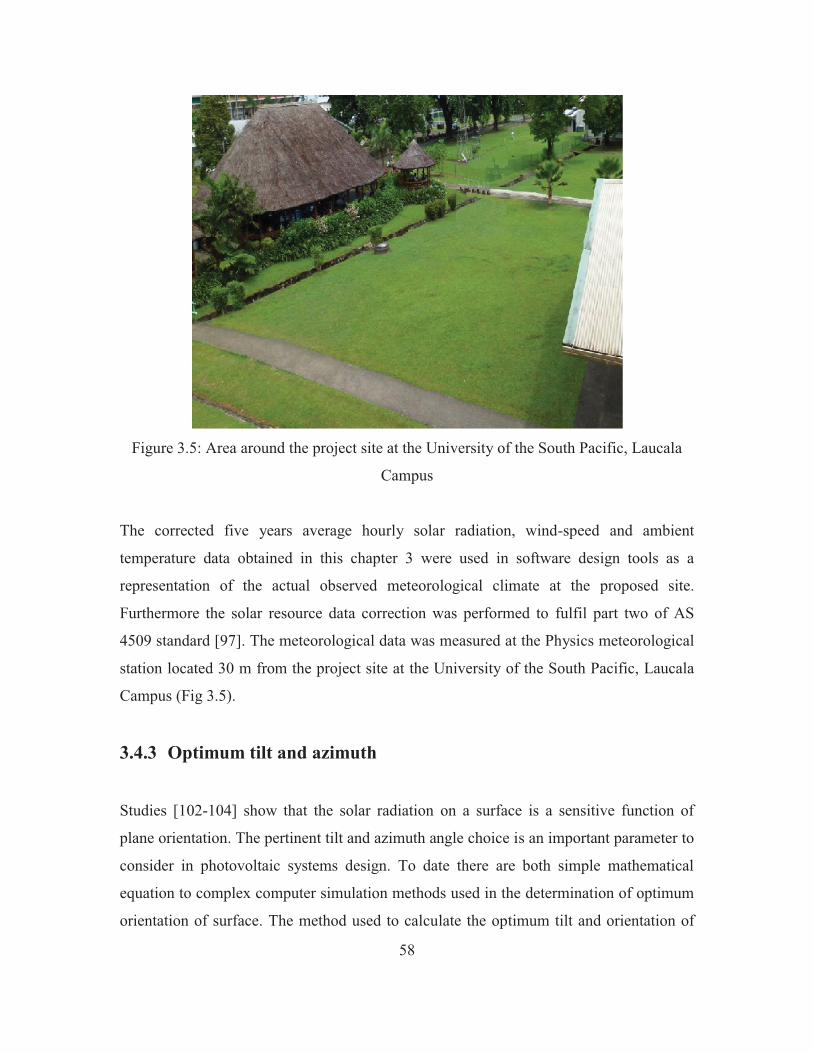
58
Figure 3.5: Area around the project site at the University of the South Pacific, Laucala
Campus
The corrected five years average hourly solar radiation, wind-speed and ambient
temperature data obtained in this chapter 3 were used in software design tools as a
representation of the actual observed meteorological climate at the proposed site.
Furthermore the solar resource data correction was performed to fulfil part two of AS
4509 standard [97]. The meteorological data was measured at the Physics meteorological
station located 30 m from the project site at the University of the South Pacific, Laucala
Campus (Fig 3.5).
3.4.3 Optimum tilt and azimuth
Studies [102-104] show that the solar radiation on a surface is a sensitive function of
plane orientation. The pertinent tilt and azimuth angle choice is an important parameter to
consider in photovoltaic systems design. To date there are both simple mathematical
equation to complex computer simulation methods used in the determination of optimum
orientation of surface. The method used to calculate the optimum tilt and orientation of
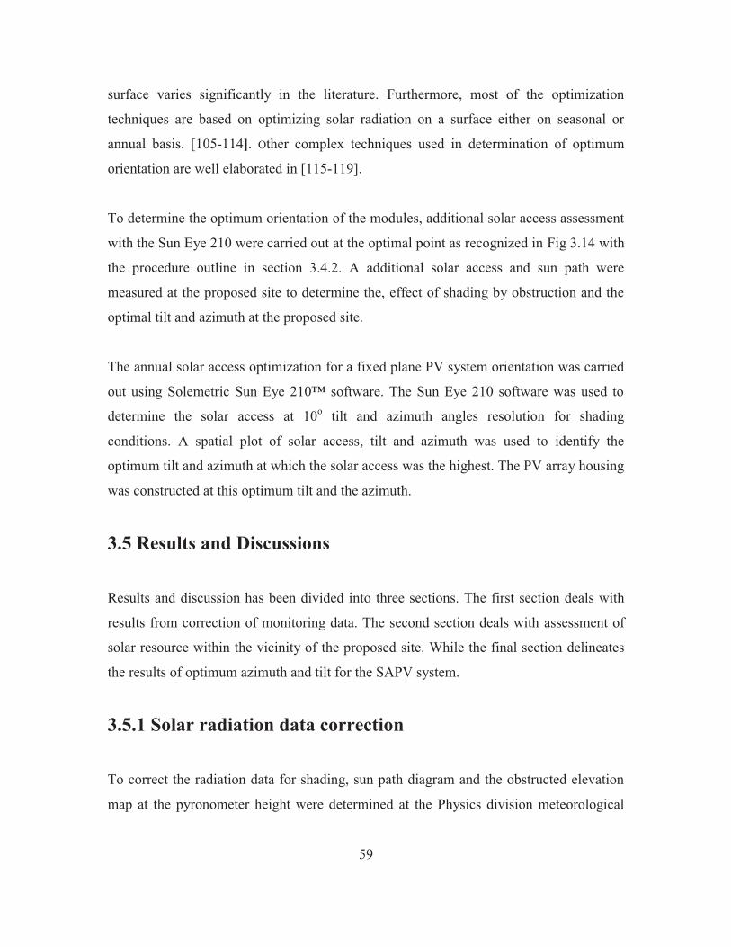
59
surface varies significantly in the literature. Furthermore, most of the optimization
techniques are based on optimizing solar radiation on a surface either on seasonal or
annual basis. [105-114]. Other complex techniques used in determination of optimum
orientation are well elaborated in [115-119].
To determine the optimum orientation of the modules, additional solar access assessment
with the Sun Eye 210 were carried out at the optimal point as recognized in Fig 3.14 with
the procedure outline in section 3.4.2. A additional solar access and sun path were
measured at the proposed site to determine the, effect of shading by obstruction and the
optimal tilt and azimuth at the proposed site.
The annual solar access optimization for a fixed plane PV system orientation was carried
out using Solemetric Sun Eye 210™ software. The Sun Eye 210 software was used to
determine the solar access at 10o tilt and azimuth angles resolution for shading
conditions. A spatial plot of solar access, tilt and azimuth was used to identify the
optimum tilt and azimuth at which the solar access was the highest. The PV array housing
was constructed at this optimum tilt and the azimuth.
3.5 Results and Discussions
Results and discussion has been divided into three sections. The first section deals with
results from correction of monitoring data. The second section deals with assessment of
solar resource within the vicinity of the proposed site. While the final section delineates
the results of optimum azimuth and tilt for the SAPV system.
3.5.1 Solar radiation data correction
To correct the radiation data for shading, sun path diagram and the obstructed elevation
map at the pyronometer height were determined at the Physics division meteorological
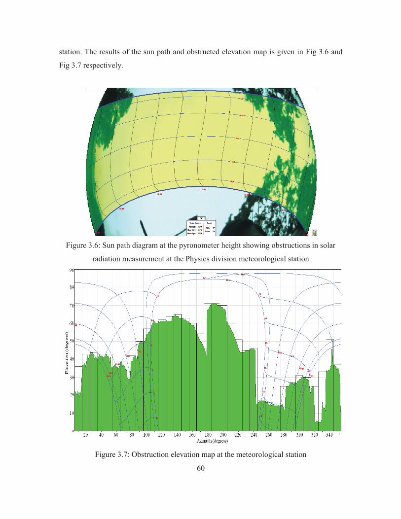
60
station. The results of the sun path and obstructed elevation map is given in Fig 3.6 and
Fig 3.7 respectively.
Figure 3.6: Sun path diagram at the pyronometer height showing obstructions in solar
radiation measurement at the Physics division meteorological station
Figure 3.7: Obstruction elevation map at the meteorological station

61
Figure 3.8: Monthly solar access at the meteorological station
From the observation of Fig 3.6 and 3.7, above, it can be concluded that the measured
solar radiation at the meteorological station has to be corrected for shading. Fig 3.7 and
Fig 3.8 shows that the pyronometer shading varies both on the monthly and hourly basis.
The results of Fig 3.8 show that pyronometer at the Physics division meteorological
station is shaded the most in June (34% shading) and the least in March and September
(7% shading). Thus, the measured solar radiation at the site has to be corrected for
shading by tress and nearby buildings.
months
jan feb mar apr may jun jul aug sep oct nov dec
Daily
Global
Solar
Radia
tion (kW
m-2 / day)
0
1
2
3
4
5
6
7
measured solar radiation (obstructed)Synthesized daily global solar radiationcorrected solar radiation
Figure 3.9: Five years averaged monthly measured, corrected and software synthesized
radiation data
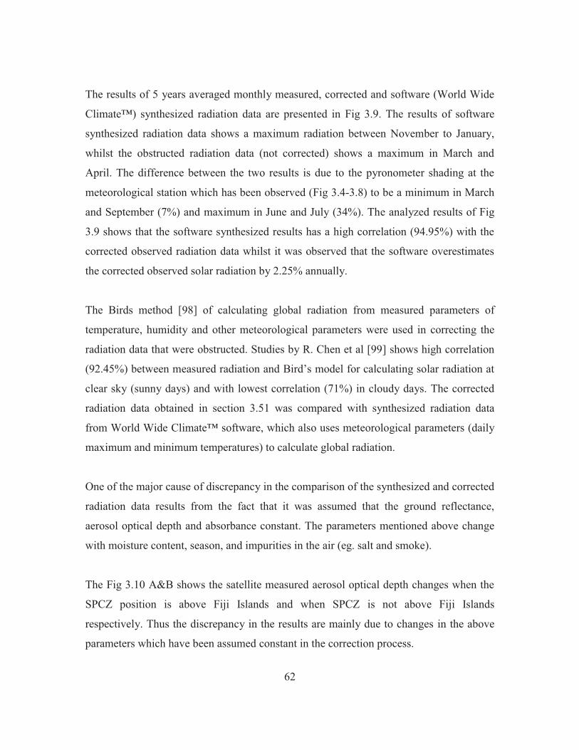
62
The results of 5 years averaged monthly measured, corrected and software (World Wide
Climate™) synthesized radiation data are presented in Fig 3.9. The results of software
synthesized radiation data shows a maximum radiation between November to January,
whilst the obstructed radiation data (not corrected) shows a maximum in March and
April. The difference between the two results is due to the pyronometer shading at the
meteorological station which has been observed (Fig 3.4-3.8) to be a minimum in March
and September (7%) and maximum in June and July (34%). The analyzed results of Fig
3.9 shows that the software synthesized results has a high correlation (94.95%) with the
corrected observed radiation data whilst it was observed that the software overestimates
the corrected observed solar radiation by 2.25% annually.
The Birds method [98] of calculating global radiation from measured parameters of
temperature, humidity and other meteorological parameters were used in correcting the
radiation data that were obstructed. Studies by R. Chen et al [99] shows high correlation
(92.45%) between measured radiation and Bird’s model for calculating solar radiation at
clear sky (sunny days) and with lowest correlation (71%) in cloudy days. The corrected
radiation data obtained in section 3.51 was compared with synthesized radiation data
from World Wide Climate™ software, which also uses meteorological parameters (daily
maximum and minimum temperatures) to calculate global radiation.
One of the major cause of discrepancy in the comparison of the synthesized and corrected
radiation data results from the fact that it was assumed that the ground reflectance,
aerosol optical depth and absorbance constant. The parameters mentioned above change
with moisture content, season, and impurities in the air (eg. salt and smoke).
The Fig 3.10 A&B shows the satellite measured aerosol optical depth changes when the
SPCZ position is above Fiji Islands and when SPCZ is not above Fiji Islands
respectively. Thus the discrepancy in the results are mainly due to changes in the above
parameters which have been assumed constant in the correction process.
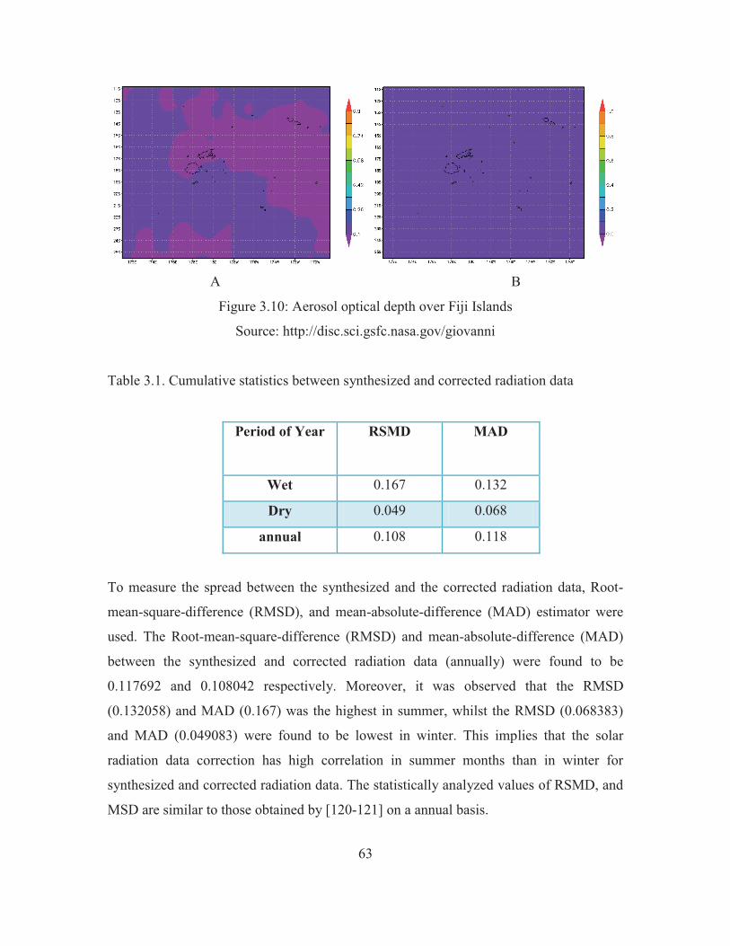
63
A B
Figure 3.10: Aerosol optical depth over Fiji Islands
Source: http://disc.sci.gsfc.nasa.gov/giovanni
Table 3.1. Cumulative statistics between synthesized and corrected radiation data
Period of Year RSMD MAD
Wet 0.167 0.132
Dry 0.049 0.068
annual 0.108 0.118
To measure the spread between the synthesized and the corrected radiation data, Root-
mean-square-difference (RMSD), and mean-absolute-difference (MAD) estimator were
used. The Root-mean-square-difference (RMSD) and mean-absolute-difference (MAD)
between the synthesized and corrected radiation data (annually) were found to be
0.117692 and 0.108042 respectively. Moreover, it was observed that the RMSD
(0.132058) and MAD (0.167) was the highest in summer, whilst the RMSD (0.068383)
and MAD (0.049083) were found to be lowest in winter. This implies that the solar
radiation data correction has high correlation in summer months than in winter for
synthesized and corrected radiation data. The statistically analyzed values of RSMD, and
MSD are similar to those obtained by [120-121] on a annual basis.
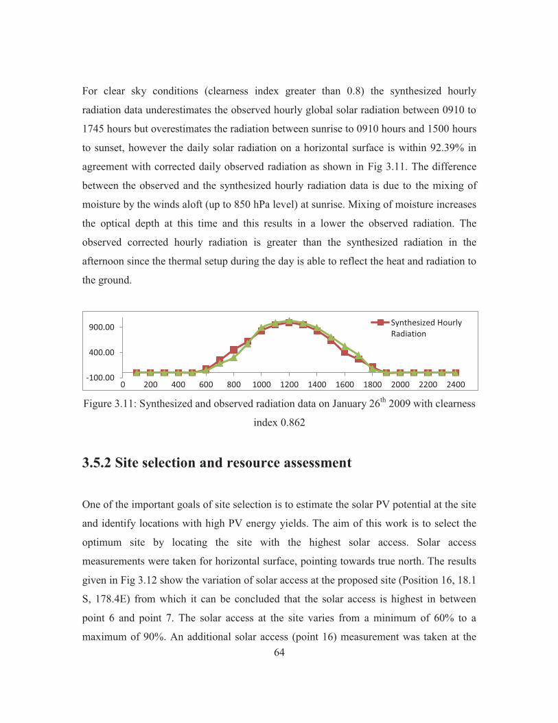
64
For clear sky conditions (clearness index greater than 0.8) the synthesized hourly
radiation data underestimates the observed hourly global solar radiation between 0910 to
1745 hours but overestimates the radiation between sunrise to 0910 hours and 1500 hours
to sunset, however the daily solar radiation on a horizontal surface is within 92.39% in
agreement with corrected daily observed radiation as shown in Fig 3.11. The difference
between the observed and the synthesized hourly radiation data is due to the mixing of
moisture by the winds aloft (up to 850 hPa level) at sunrise. Mixing of moisture increases
the optical depth at this time and this results in a lower the observed radiation. The
observed corrected hourly radiation is greater than the synthesized radiation in the
afternoon since the thermal setup during the day is able to reflect the heat and radiation to
the ground.
Figure 3.11: Synthesized and observed radiation data on January 26th 2009 with clearness
index 0.862
3.5.2 Site selection and resource assessment
One of the important goals of site selection is to estimate the solar PV potential at the site
and identify locations with high PV energy yields. The aim of this work is to select the
optimum site by locating the site with the highest solar access. Solar access
measurements were taken for horizontal surface, pointing towards true north. The results
given in Fig 3.12 show the variation of solar access at the proposed site (Position 16, 18.1
S, 178.4E) from which it can be concluded that the solar access is highest in between
point 6 and point 7. The solar access at the site varies from a minimum of 60% to a
maximum of 90%. An additional solar access (point 16) measurement was taken at the
-100.00
400.00
900.00
0 200 400 600 800 1000 1200 1400 1600 1800 2000 2200 2400
Synthesized HourlyRadiation
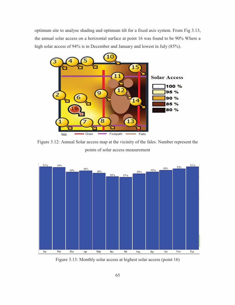
65
optimum site to analyse shading and optimum tilt for a fixed axis system. From Fig 3.13,
the annual solar access on a horizontal surface at point 16 was found to be 90% Where a
high solar access of 94% is in December and January and lowest in July (85%).
Figure 3.12: Annual Solar access map at the vicinity of the fales. Number represent the
points of solar access measurement
Figure 3.13: Monthly solar access at highest solar access (point 16)
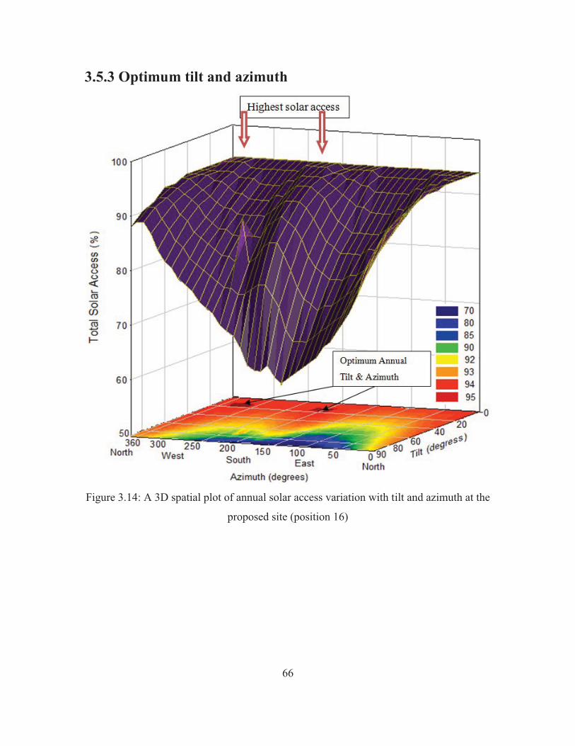
66
3.5.3 Optimum tilt and azimuth
Figure 3.14: A 3D spatial plot of annual solar access variation with tilt and azimuth at the
proposed site (position 16)
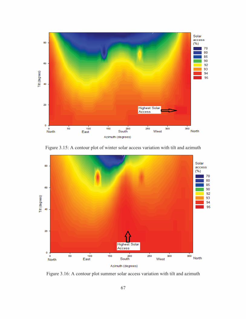
67
Figure 3.15: A contour plot of winter solar access variation with tilt and azimuth
Figure 3.16: A contour plot summer solar access variation with tilt and azimuth
68
A 3D spatial plot as shown in Fig 3.14 was used to determine the optimum tilt and
azimuth of the solar panel orientation for high annual energy yield. The results in Fig
3.15 and 3.16 show the annual, summer and winter optimization of tilt and azimuth angle
respectively. The results of Fig 3.14 show that there are two optimum orientations (solar
access of 95%) of the solar modules. The first optimum orientation lies at a tilt of 13-17°
and 320-340° azimuth whilst the second optimum tilt is at 15-23° and 180-210° azimuth.
To refine the selection of the optimum orientation the result of Fig 3.15 & 3.16 were
used. The results of Fig 3.16 shows the summer optimization of 20-30° tilt and 190-200°
azimuth whilst the results for winter (Fig 3.15) optimization show a 15-20° tilt and 330-
350° azimuth. The University is on semester break in summer (December to mid
February) and has lower load for laptop system, thus the winter orientation was chosen as
the optimum orientation of the modules.
Studies by [122-127] has reported that the optimum tilt of high insolation is at the latitude
of the location for a equator facing system. For this study the optimum tilt obtained from
the shade analysis varies within the limits of ± 10 degrees latitude, whilst the value of the
azimuth has shifted from equator facing (N= zero degrees) to facing NNW due to shading
by the fales between winter and summer season.
The optimum tilt and azimuth angles were further refined to cater for the effects of
morning and afternoon cloudiness. The Anova test was used to statistically analyse if
there is variation between the morning and afternoon cloudiness. Trade winds persist
over Fiji islands. On the windward side of the two major islands, moisture converges over
the rugged terrain and rains on the eastern side of the two islands.
It was observed that F < Fcritical at α = 5% and degrees of freedom of 4329 (Table 3.2).
Thus, this implies that we accept the null hypothesis and conclude that there is no
significant difference between morning and afternoon cloudiness. Since there is no
correlation between morning and afternoon cloudiness the optimum tilt obtained above is
69
same as if an optimization with respect to morning and afternoon cloudiness on the
variation of global radiation would have had been carried out [127].
Table 3.2: ANOVA results for morning and afternoon cloudiness
Source of
Variation SS df MS F P-value F crit
Between
Groups 260.9319 1 260.9319 0.004524 0.946375 3.842533
Within Groups 4.99E+08 4328 57676.45
Total 4.99E+08 4329
3.6 Conclusion
The annual corrected horizontal radiation at the site is 4.8 kW/m2. The area within the
vicinity of the fales that has the highest annual solar access is marked as position 16 in
Fig 3.13. The optimum orientation of tilt and azimuth for highest annual solar radiation at
the site were found to be 15-20 degrees and 330-350 degrees respectively. The annual
average solar access to direct radiation on a clear day at the site was found to be 90.3%.
Chapter 5 uses the optimum orientations and the corrected solar radiation data on
monthly bases to design a optimum performing SAPV system for light and laptop system.
70
Chapter 4
4.0 Performance testing and monitoring
4.1 Introduction
The lack of standard methods of performance evaluation and absence of performance
monitoring infrastructure hinders the utilization of PV systems in energy generation
[128]. The need for component performance data is essential in designing of optimal PV
system based on the resources and performance of the individual components.
The amount of power produced by a SAPV system is dependent on the meteorological
conditions at the site of installation and the performance of each of the components
integrated to form a SAPV [129.]. Field performance data of SAPV components is
essential for system designers and installers in designing an optimal system. Field
monitoring of performance data enables PV installers and system designers to design PV
systems that maximize revenue generation by reducing operation and maintenance costs
[130]. The data monitoring helps project developers to correlate PV System performance
and maintenance issues to weather conditions and energy output. Prior knowledge of PV
system performance data saves time, money and increases investment confidence in PV
systems as alternative economical form of energy.
Continuous monitoring data provides the preliminary level of information that is helpful
in rectifying the sources of problems encountered in daily operation of PV systems. The
data can also be used to inform manufactures regarding product improvement. In
addition, the monitoring of a PV system provides knowledge and evidence of actual
performance of the systems. Furthermore, the field performance data is useful to
designers who are guaranteed a certain level of system performance based on software
simulation of PV system.
71
This chapter reviews the current international and organizational, guidelines and quality
assessment procedures used to assess and monitor the performance of the SAPV system
and its components. Therefore this chapter aims to test and derive the necessary
information needed to increases the accuracy of modelling and analysis of SAPV system
by studying the behaviour and response of each component of a SAPV system [131].
4.2 Inverters
The operating principle, algorithm and the complexity of power electronic circuitry in
inverters determines the effectiveness of inverters in PV systems. To date grid tie, true
sine and modified sine are three main types of inverters mostly used in PV applications.
Use of the three types of inverter in PV system is dependent on the load complexity, cost
and the type of SAPV system considered [132].
Modified sine wave inverters are low cost and low efficiency inverters. They are mostly
used in less sensitive and non-specialized application such as fluorescent lights, audio
equipments, TV. The output from the modified sine wave inverter is an approximation of
sine wave but with a square wave in a H-bridge circuit arrangement [133]. True sine
wave inverters are also known as pure sine wave inverters. The output from these inverter
are sinusoidal and there is less than 3% THD which makes it useful in precise and
specialized applications such as computers and laser printers [134].
Grid tied inverters have a pure sine inverter and are designed to deliver electricity to the
electrical grid. These inverters have the capability of automatically synchronizing
themselves with the grid voltage, phase and frequency [133].

72
4.2.1 Inverter Testing
The UL 1741 [135], IEEE STD 1526-2003 [136], DIN VDE 0126-1-1 [137], IEC 61683
[138], IEC 62109-1 [139], IEC 62109-2 [140], AS/NZS 5603:2009 [141] and PQC PVRS
8:2001 [142] are some of the international standards that are used to access the safety and
operational specifications of inverters in SAPV systems. These standards also outline the
performance requirement of inverters in SAPV application [143]. The aim of this testing
procedure is determine the efficiency of TBS600 and TBS1000 inverters, and understand
the behaviour of the two inverters in SAPV system under different load conditions.
Two true sine TBS brand (PS 1000-12 and PS 600-12) dc to ac inverters were tested for
Total Harmonic Distortion (THD), power factor and efficiency of dc to ac conversion.
The inverter specification is given in table 4.1.
A light bulb bank was used to supply resistive loads to each of the inverters. The loads
were varied by switching on and increasing the number of light bulbs in the load. A
FLUKE 434 power quality analyzer was used to analyse the power quality, efficiency and
total harmonic distortion from the input and output of the inverter. Specifications of
FLUKE 434 power quality analyzer is given in the appendix 4A. The experimental setup
is shown in fig 4.1.
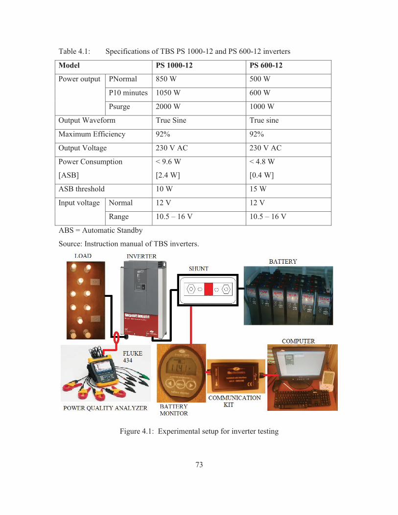
73
Table 4.1: Specifications of TBS PS 1000-12 and PS 600-12 inverters
Model PS 1000-12 PS 600-12
Power output PNormal 850 W 500 W
P10 minutes 1050 W 600 W
Psurge 2000 W 1000 W
Output Waveform True Sine True sine
Maximum Efficiency 92% 92%
Output Voltage 230 V AC 230 V AC
Power Consumption
[ASB]
< 9.6 W
[2.4 W]
< 4.8 W
[0.4 W]
ASB threshold 10 W 15 W
Input voltage Normal 12 V 12 V
Range 10.5 – 16 V 10.5 – 16 V
ABS = Automatic Standby
Source: Instruction manual of TBS inverters.
Figure 4.1: Experimental setup for inverter testing
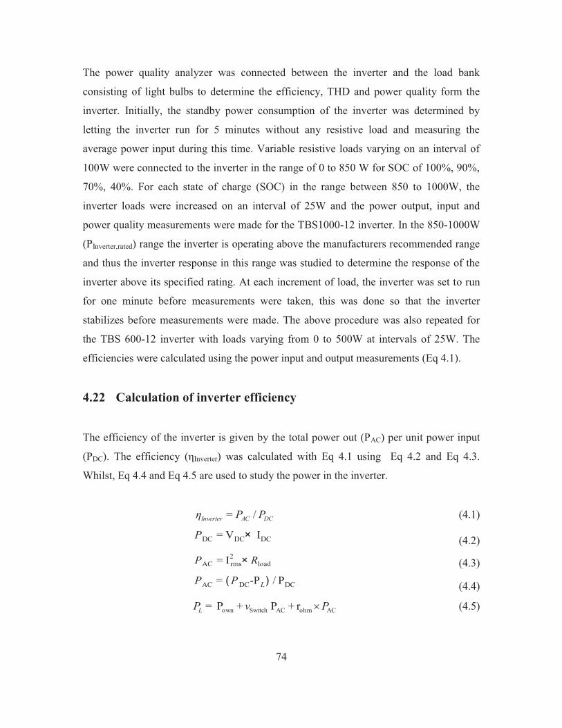
74
The power quality analyzer was connected between the inverter and the load bank
consisting of light bulbs to determine the efficiency, THD and power quality form the
inverter. Initially, the standby power consumption of the inverter was determined by
letting the inverter run for 5 minutes without any resistive load and measuring the
average power input during this time. Variable resistive loads varying on an interval of
100W were connected to the inverter in the range of 0 to 850 W for SOC of 100%, 90%,
70%, 40%. For each state of charge (SOC) in the range between 850 to 1000W, the
inverter loads were increased on an interval of 25W and the power output, input and
power quality measurements were made for the TBS1000-12 inverter. In the 850-1000W
(PInverter,rated) range the inverter is operating above the manufacturers recommended range
and thus the inverter response in this range was studied to determine the response of the
inverter above its specified rating. At each increment of load, the inverter was set to run
for one minute before measurements were taken, this was done so that the inverter
stabilizes before measurements were made. The above procedure was also repeated for
the TBS 600-12 inverter with loads varying from 0 to 500W at intervals of 25W. The
efficiencies were calculated using the power input and output measurements (Eq 4.1).
4.22 Calculation of inverter efficiency
The efficiency of the inverter is given by the total power out (PAC) per unit power input
(PDC). The efficiency (ηInverter) was calculated with Eq 4.1 using Eq 4.2 and Eq 4.3.
Whilst, Eq 4.4 and Eq 4.5 are used to study the power in the inverter.
DCACInverter PP=η / (4.1)
PDC = VDC× IDC (4.2)
PAC = Irms2 × Rload (4.3)
PAC = ( PDC-PL) / PDC (4.4)
ACohmACSwitchown r+ P + P = PνPL � (4.5)

75
Where,
PAC is the AC power output of the inverter.
Rload is the resistance of the load.
PDC is the inverter dc input power
PL is the power lost in conversion from DC to AC.
Pown is the dc loss in the inverter.
νSwitch is the semiconductor switch loss
rohm is the ohmic loss in the coils and wires.
The individual components of the inverter loss were calculated by using Schmidt and
Sauer [143] method for algebraic manipulation of efficiency. The efficiency at 40%,
90% and 100% of the rated power output were used in the Schmidt and Sauer equations.
The Schmidt and Sauer algebraic expression for efficiency is given in Eq 4.6-4.8. The
efficiency, power quality and loss components determined in this section, are latter used
in modelling inverter performance in PV-DesignPro-STM software design tools.
)PηP(ηPPηη+)Pη+P(ηPηPη))PηP(ηηη+)PηP(ηη+)η(ηP(ηPPP=Pown
332232323322112
121
3322322223
231321
21321
����� (4.6)
)PηP)(ηPηP)(ηPηP(η)P(PPη+PPηη)PP+P(ηPη+)PηP(ηPη+)PPPηP(ηPη
=νSwitch223333112211
122
323
232
2323133
22
22
22
22
23
2311323322
21
21
����������
(4.7)
)PηP(ηPPηη+)Pη+P(ηPηPη)P(PPη+)P(PPη+)P(PPη=rohm
223332323322112
121
213333223211
�����
(4.8)
Where,
P1, P2, P3 are three different DC power inputs for the inverter.
1η , 2η , 3η are the respective efficiencies of different DC powers inputs.
76
4.23 Inverter performance monitoring and control
Real time inverter performance monitoring provides accurate inverter states and health of
the inverter. The real time monitored data provides preliminary level of inverter
diagnostic information [144].
The PS1000-12 TBS inverter performance was monitored by the DashboardTM software
program linked to the computer by the optically isolated TBS Link as shown in fig4.2.
The real time inverter status and power related quantities were measured and recorded on
a dedicated computer. DashboardTM software was used to control the operation of the
inverter, and to protect the battery in case of low state of charge. Inverter control program
summary is given in the Table 4.2. Separate and isolated monitoring and control of the
inverter performance was also carried out with the use of universal remote control system
to manually override the inverter operation if the computer controlled program fails to
operate. Details of universal remote control display and control overview are attached in
appendix 4B.
To protect the battery from deep discharge, the PS1000-12 inverter computer control
algorithm in Dashboard TM software was programmed to shut down the PS100-12 inverter
if the battery SOC is less than 40% and in condition of over loading beyond the rated
inverter capacity as detailed in table 4.1. For the PS600-12 inverter, there was no such
setting to protect the battery from deep discharge but had a battery alarm system to alert
the technicians in condition of low battery SOC.
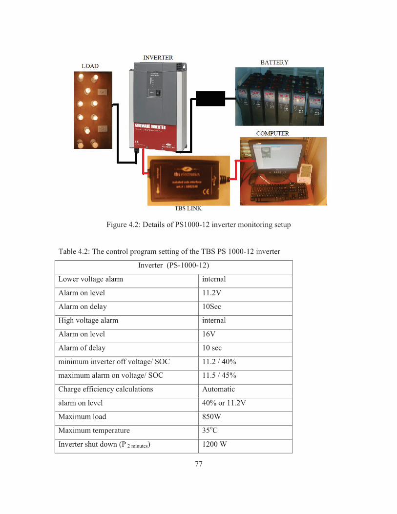
77
Figure 4.2: Details of PS1000-12 inverter monitoring setup
Table 4.2: The control program setting of the TBS PS 1000-12 inverter
Inverter (PS-1000-12)
Lower voltage alarm internal
Alarm on level 11.2V
Alarm on delay 10Sec
High voltage alarm internal
Alarm on level 16V
Alarm of delay 10 sec
minimum inverter off voltage/ SOC 11.2 / 40%
maximum alarm on voltage/ SOC 11.5 / 45%
Charge efficiency calculations Automatic
alarm on level 40% or 11.2V
Maximum load 850W
Maximum temperature 35oC
Inverter shut down (P 2 minutes) 1200 W
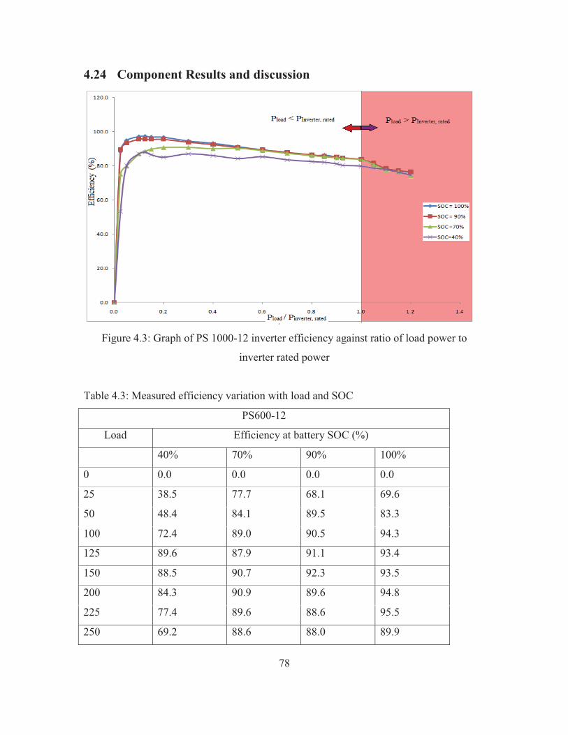
78
4.24 Component Results and discussion
Figure 4.3: Graph of PS 1000-12 inverter efficiency against ratio of load power to
inverter rated power
Table 4.3: Measured efficiency variation with load and SOC
PS600-12
Load Efficiency at battery SOC (%)
40% 70% 90% 100%
0 0.0 0.0 0.0 0.0
25 38.5 77.7 68.1 69.6
50 48.4 84.1 89.5 83.3
100 72.4 89.0 90.5 94.3
125 89.6 87.9 91.1 93.4
150 88.5 90.7 92.3 93.5
200 84.3 90.9 89.6 94.8
225 77.4 89.6 88.6 95.5
250 69.2 88.6 88.0 89.9
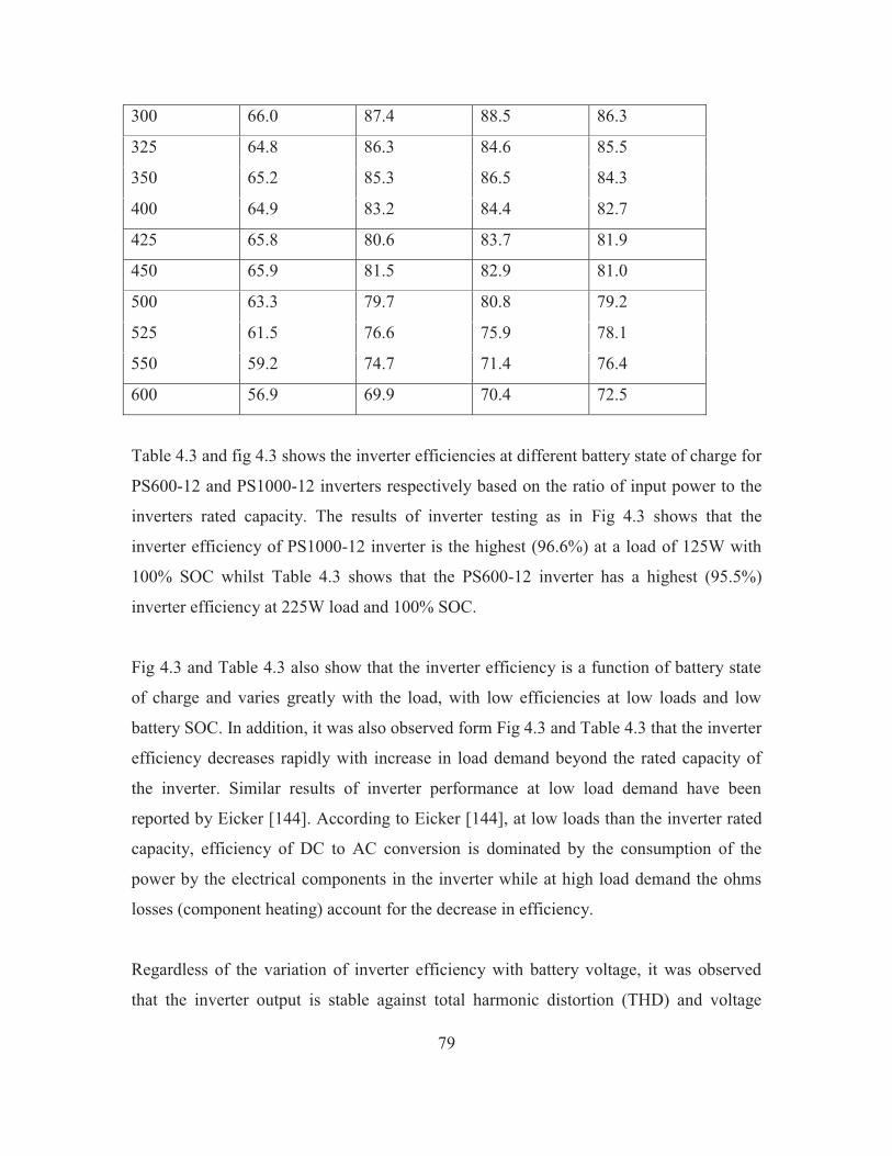
79
300 66.0 87.4 88.5 86.3
325 64.8 86.3 84.6 85.5
350 65.2 85.3 86.5 84.3
400 64.9 83.2 84.4 82.7
425 65.8 80.6 83.7 81.9
450 65.9 81.5 82.9 81.0
500 63.3 79.7 80.8 79.2
525 61.5 76.6 75.9 78.1
550 59.2 74.7 71.4 76.4
600 56.9 69.9 70.4 72.5
Table 4.3 and fig 4.3 shows the inverter efficiencies at different battery state of charge for
PS600-12 and PS1000-12 inverters respectively based on the ratio of input power to the
inverters rated capacity. The results of inverter testing as in Fig 4.3 shows that the
inverter efficiency of PS1000-12 inverter is the highest (96.6%) at a load of 125W with
100% SOC whilst Table 4.3 shows that the PS600-12 inverter has a highest (95.5%)
inverter efficiency at 225W load and 100% SOC.
Fig 4.3 and Table 4.3 also show that the inverter efficiency is a function of battery state
of charge and varies greatly with the load, with low efficiencies at low loads and low
battery SOC. In addition, it was also observed form Fig 4.3 and Table 4.3 that the inverter
efficiency decreases rapidly with increase in load demand beyond the rated capacity of
the inverter. Similar results of inverter performance at low load demand have been
reported by Eicker [144]. According to Eicker [144], at low loads than the inverter rated
capacity, efficiency of DC to AC conversion is dominated by the consumption of the
power by the electrical components in the inverter while at high load demand the ohms
losses (component heating) account for the decrease in efficiency.
Regardless of the variation of inverter efficiency with battery voltage, it was observed
that the inverter output is stable against total harmonic distortion (THD) and voltage
80
fluction. The measured results of total harmonic distortion shows that the maximum THD
varied by 1.03% for an average of 10 cycles of the waveform, whilst the maximum
voltage fluction of 0.87% and 0.89% was observed for the PS1000-12, PS600-12 inverter
respectively.
Schmidt and Sauer’s equations were used to solve the individual components of average
inverter loss as stated in Eq 4.5. The inverter loss parameters vary with battery SOC thus
the values determined had been averaged for a simpler simulation. The parameters of
Pown, νSwitch and rohm for the PS1000-12 inverter were found to be 23.8W, 0.26 and 0.015
respectively. Whilst for the PS600-12 inverter the average inverter loss parameters of
Pown+ νSwitch and rohm were found to be 21.4W, 0.32 and 0.063 respectively.
The absolute maximum inverter efficiency was observed at the point where the inverter
losses are absolute minimum. At load demand above the rated power capacity
(PLoad>PInverter,rated) of the inverter, the efficiency depends on the inverter overloading
behaviour circuit. In this region of inverter operation the inverter loss is observed to be a
relative maximum and overheating of electrical components has been reported to be a
major cause of this loss [143]. To reduce inverter overheating, the inverter control
algorithm is generally designed to maintain inverter temperature of less than 35oC [143].
The forced cooling technique, by thermostatically operated fan, is switched on at inverter
temperature of 30oC or more.
4.3 Battery
The electric energy generated by the PV array cannot be always used directly in SAPV
system as it is produced since the time of demand and generation are not in-phase all the
time [145]. To cater for the phase difference in demand and generation Energy storage in
SAPV system plays a vital role in circulating energy between the load and the demand.
Deep and shallow cycle batteries are the two types batteries used in PV systems to store
81
energy. The use of battery in SAPV application is limited to cost, reliability and design
performance characteristics [146].
Shallow cycle batteries are cheaper than deep cycle batteries and are design for small
discharge applications. These batteries are used to deliver high discharge currents for
short time and are primarily use in PV system to deliver energy to electrical loads at
stable voltage and current by suppressing transient in load demands [146].
Deep cycle batteries have a longer lifetime and are generally designed for SAPV
application. These batteries are designed to withstand frequent deep charge discharge
cycles and temperature extremes much better than shallow cycle batteries [145-147].
Amongst the deep discharge batteries, the most common battery types are flooded lead-
acid, captive electrolyte lead acid (VRLA) and nickel-cadmium, Nickel-Metal Hydride
and Lithium ion battery [147]. The electrolytic material and the manufacturing
technology in each of the three battery type determines the cell chemical reaction and
battery performance characteristics [146].
Battery performance in SAPV system is accredited to battery design and PV system
operational conditions. Batteries experience a wide range of variable operational
conditions in SAPV applications, including varying frequency and depth of
charge/discharge cycles, temperature extremes, rates of charge and discharge, and the
methods and limits of charge regulation [146]. These varying operating conditions make
it very difficult to precisely predict battery performance and lifetime of batteries in SAPV
systems. Battery manufacturers’ specifications often provides scarce information for
detailed simulation of batteries in SAPV system designer software. The performance data
presented by battery manufacturers are based on tests conducted at specified test
conditions which are often not representative of battery operation in actual SAPV system
[145].
82
4.31 Battery testing
Amongst the most common techniques of battery testing are the EP0762135 A2 [148],
WO96/35522 [149], U.S. Pat No.5596260 [150], BIS IS 15549:2005 [151] and IEEE
Standard 450™ [152] which uses a broad range of techniques, ranging from artificial
neural network to algorithmic determination of battery performance, which are well
documented in [153]. The above battery testing standards have their own emphases on
special test parameters for different charge and discharge conditions. While there exists
some differences between the methods of evaluating battery performance standards, there
are two most common modes of evaluating battery charging and discharging efficiency.
Constant current or constant power discharge modes are the two most frequently utilized
procedures for determination of battery performance. The method of battery performance
evaluation, monitoring and control algorithm in present testing procedure has been
designed in close compliance with IEEE-450™ [152] and IEC- 62093™ [153] standards.
Therefore this study aims to determine the battery charge and discharge efficiency under
Fiji’s environmental conditions. The constant power mode of discharge efficiency testing
was chosen over the constant current method of discharge efficiency determination for
the battery banks since the inverter maintains a constant power input and constant power
output to the load regardless of the fluctuation of battery voltage and current during
discharging. Whilst, the constant voltage method of charging efficiency evaluation was
chosen over the constant current method since the charge controller maintains a constant
battery voltage during charging. Details of charge controller voltage set-points and
charging algorithms are provided in section 4.4
A 12volts Tudor 1000 Ah brand battery bank was tested for efficiency of charging and
discharging. The battery bank consisted of six cells arranged in series with an open
circuit voltage of 12V. The cell specification is given in table 4.4.
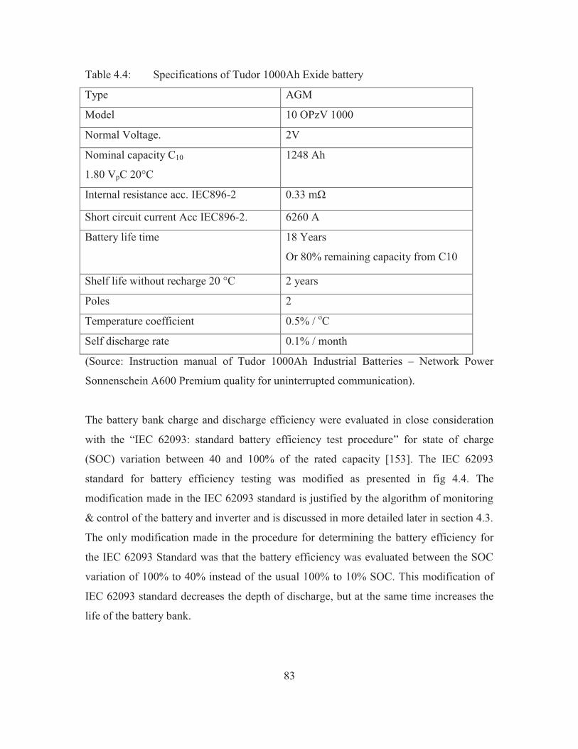
83
Table 4.4: Specifications of Tudor 1000Ah Exide battery
Type AGM
Model 10 OPzV 1000
Normal Voltage. 2V
Nominal capacity C10
1.80 VpC 20°C
1248 Ah
Internal resistance acc. IEC896-2 0.33 mΩ
Short circuit current Acc IEC896-2. 6260 A
Battery life time 18 Years
Or 80% remaining capacity from C10
Shelf life without recharge 20 °C 2 years
Poles 2
Temperature coefficient 0.5% / oC
Self discharge rate 0.1% / month
(Source: Instruction manual of Tudor 1000Ah Industrial Batteries – Network Power
Sonnenschein A600 Premium quality for uninterrupted communication).
The battery bank charge and discharge efficiency were evaluated in close consideration
with the “IEC 62093: standard battery efficiency test procedure” for state of charge
(SOC) variation between 40 and 100% of the rated capacity [153]. The IEC 62093
standard for battery efficiency testing was modified as presented in fig 4.4. The
modification made in the IEC 62093 standard is justified by the algorithm of monitoring
& control of the battery and inverter and is discussed in more detailed later in section 4.3.
The only modification made in the procedure for determining the battery efficiency for
the IEC 62093 Standard was that the battery efficiency was evaluated between the SOC
variation of 100% to 40% instead of the usual 100% to 10% SOC. This modification of
IEC 62093 standard decreases the depth of discharge, but at the same time increases the
life of the battery bank.
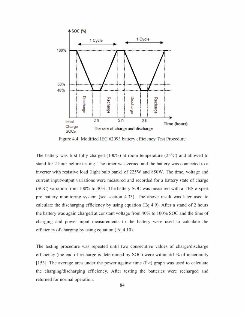
84
Figure 4.4: Modified IEC 62093 battery efficiency Test Procedure
The battery was first fully charged (100%) at room temperature (25oC) and allowed to
stand for 2 hour before testing. The timer was zeroed and the battery was connected to a
inverter with resistive load (light bulb bank) of 225W and 850W. The time, voltage and
current input/output variations were measured and recorded for a battery state of charge
(SOC) variation from 100% to 40%. The battery SOC was measured with a TBS e-xpert
pro battery monitoring system (see section 4.33). The above result was later used to
calculate the discharging efficiency by using equation (Eq 4.9). After a stand of 2 hours
the battery was again charged at constant voltage from 40% to 100% SOC and the time of
charging and power input measurements to the battery were used to calculate the
efficiency of charging by using equation (Eq 4.10).
The testing procedure was repeated until two consecutive values of charge/discharge
efficiency (the end of recharge is determined by SOC) were within ±3 % of uncertainty
[153]. The average area under the power against time (P-t) graph was used to calculate
the charging/discharging efficiency. After testing the batteries were recharged and
returned for normal operation.

85
4.32 Calculation of battery efficiency
The efficiency of battery charging is given by the ratio of energy stored in the battery to
the energy input during charging (Eq 4.9). Whilst the efficiency of battery discharging is
given by the ratio of energy output from the battery to the energy stored during charging
Eq 4.10, which is expressed in terms of energy output divided by energy input.
inin
Storagearg
area VI = =P
)(E
Eη ingCh ( 4.9)
)(EEη ingDisch area VI
P = = out
stored
outarg
(4.10)
Where: ηDischarging , ηCharging is the efficiency of discharging and charging of the battery
respectively.
EStorage is the chemical energy stored in the battery.
Ein is the energy input to the battery.
Eout is the energy output of the battery.
VI(area) is the area under the voltage against current graph calculated using Riemann
method.
Pin is the power input to the battery.
Pout is the power output from the battery.
4.33 Battery performance monitoring and control
To date, there are standards design to monitor the operation of the batteries for VRLA
and flooded batteries (IEC/TR 62060 2001, and IEC/TR 61431 1995) [154], [155], but
there are few standards designed to monitor and control the operation of the AGM battery
[156]. In this work, the battery monitoring and control system were designed in close
compliance with IEA PVPS T3-13: 2003 [131] and IEEE 450™ standard procedures for
battery monitoring and control systems.
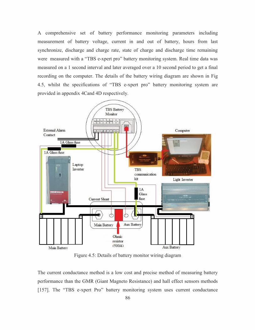
86
A comprehensive set of battery performance monitoring parameters including
measurement of battery voltage, current in and out of battery, hours from last
synchronize, discharge and charge rate, state of charge and discharge time remaining
were measured with a “TBS e-xpert pro” battery monitoring system. Real time data was
measured on a 1 second interval and later averaged over a 10 second period to get a final
recording on the computer. The details of the battery wiring diagram are shown in Fig
4.5, whilst the specifications of “TBS e-xpert pro” battery monitoring system are
provided in appendix 4Cand 4D respectively.
Figure 4.5: Details of battery monitor wiring diagram
The current conductance method is a low cost and precise method of measuring battery
performance than the GMR (Giant Magneto Resistance) and hall effect sensors methods
[157]. The “TBS e-xpert Pro” battery monitoring system uses current conductance

87
method to determine the battery state of charge, current in and out of battery and open
circuit voltage for the lighting battery and laptop charging battery voltage. The lighting
battery SOC and voltage variation measurement for the lighting battery were recorded on
a 10 seconds interval and later used for calibrating the laptop charging battery voltage to
determine the SOC for the laptop charging battery from the measured values of laptop
charging battery voltage.
Open circuit voltage measurement technique was used to calibrate the laptop charging
battery performance with respect to lighting battery operation. Firstly the lighting battery
voltage, current and SOC characteristic curves were determined from the current
conductance method. Then, the results were used to calibrate the open circuit voltage
measurement with the SOC of the laptop charging battery. The laptop charging battery
SOC, current input/output and remaining discharge time of the battery were determined
from the measured value of laptop charging battery open circuit voltage and characteristic
curve (SOC variation with VOpen Circuit ) of the lighting battery.
4.34 Battery Monitoring System
Real time battery performance monitoring provides accurate battery SOC and health of
the battery [158]. The monitored data is used in the implementation of the control
strategies to prevent overcharging or over-discharging of batteries in PV system. The
monitoring and control program setting are stated in table 4.5.
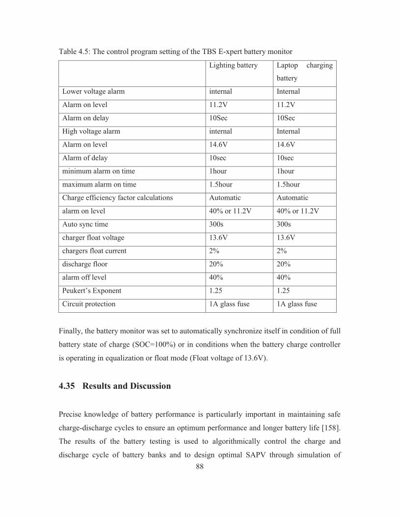
88
Table 4.5: The control program setting of the TBS E-xpert battery monitor
Lighting battery Laptop charging
battery
Lower voltage alarm internal Internal
Alarm on level 11.2V 11.2V
Alarm on delay 10Sec 10Sec
High voltage alarm internal Internal
Alarm on level 14.6V 14.6V
Alarm of delay 10sec 10sec
minimum alarm on time 1hour 1hour
maximum alarm on time 1.5hour 1.5hour
Charge efficiency factor calculations Automatic Automatic
alarm on level 40% or 11.2V 40% or 11.2V
Auto sync time 300s 300s
charger float voltage 13.6V 13.6V
chargers float current 2% 2%
discharge floor 20% 20%
alarm off level 40% 40%
Peukert’s Exponent 1.25 1.25
Circuit protection 1A glass fuse 1A glass fuse
Finally, the battery monitor was set to automatically synchronize itself in condition of full
battery state of charge (SOC=100%) or in conditions when the battery charge controller
is operating in equalization or float mode (Float voltage of 13.6V).
4.35 Results and Discussion
Precise knowledge of battery performance is particularly important in maintaining safe
charge-discharge cycles to ensure an optimum performance and longer battery life [158].
The results of the battery testing is used to algorithmically control the charge and
discharge cycle of battery banks and to design optimal SAPV through simulation of
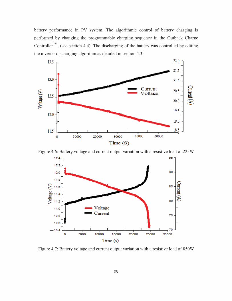
89
battery performance in PV system. The algorithmic control of battery charging is
performed by changing the programmable charging sequence in the Outback Charge
ControllerTM, (see section 4.4). The discharging of the battery was controlled by editing
the inverter discharging algorithm as detailed in section 4.3.
Figure 4.6: Battery voltage and current output variation with a resistive load of 225W
Figure 4.7: Battery voltage and current output variation with a resistive load of 850W
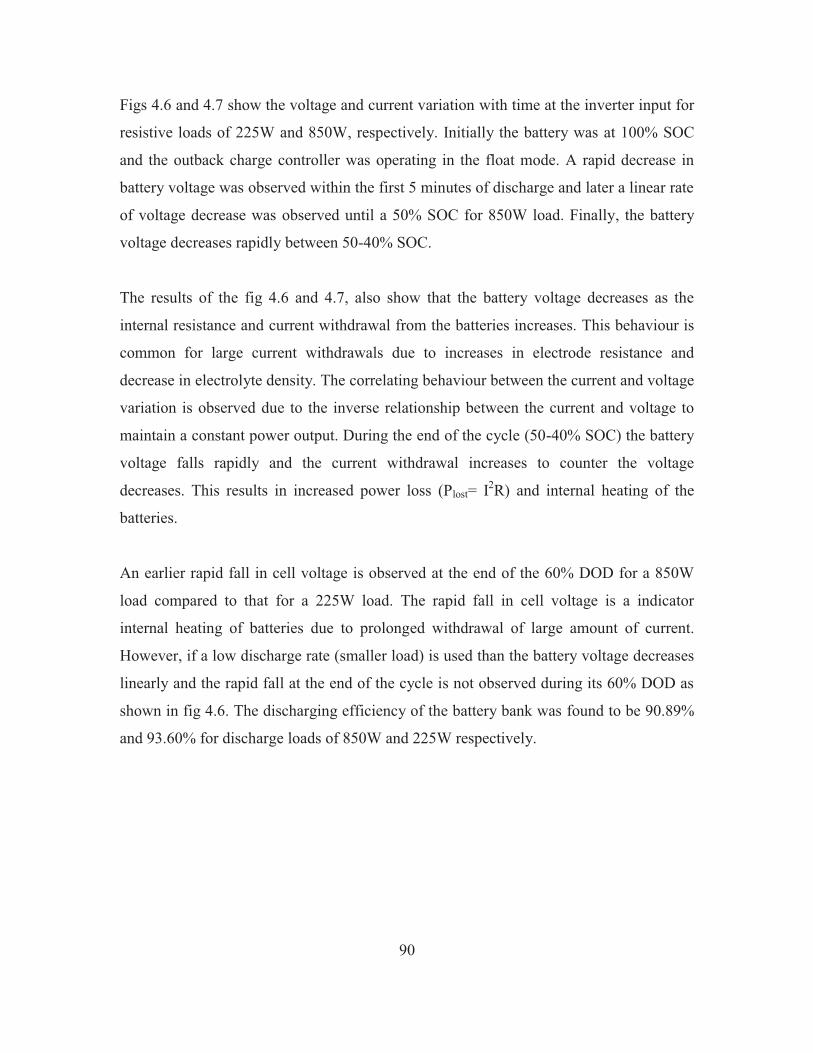
90
Figs 4.6 and 4.7 show the voltage and current variation with time at the inverter input for
resistive loads of 225W and 850W, respectively. Initially the battery was at 100% SOC
and the outback charge controller was operating in the float mode. A rapid decrease in
battery voltage was observed within the first 5 minutes of discharge and later a linear rate
of voltage decrease was observed until a 50% SOC for 850W load. Finally, the battery
voltage decreases rapidly between 50-40% SOC.
The results of the fig 4.6 and 4.7, also show that the battery voltage decreases as the
internal resistance and current withdrawal from the batteries increases. This behaviour is
common for large current withdrawals due to increases in electrode resistance and
decrease in electrolyte density. The correlating behaviour between the current and voltage
variation is observed due to the inverse relationship between the current and voltage to
maintain a constant power output. During the end of the cycle (50-40% SOC) the battery
voltage falls rapidly and the current withdrawal increases to counter the voltage
decreases. This results in increased power loss (Plost= I2R) and internal heating of the
batteries.
An earlier rapid fall in cell voltage is observed at the end of the 60% DOD for a 850W
load compared to that for a 225W load. The rapid fall in cell voltage is a indicator
internal heating of batteries due to prolonged withdrawal of large amount of current.
However, if a low discharge rate (smaller load) is used than the battery voltage decreases
linearly and the rapid fall at the end of the cycle is not observed during its 60% DOD as
shown in fig 4.6. The discharging efficiency of the battery bank was found to be 90.89%
and 93.60% for discharge loads of 850W and 225W respectively.
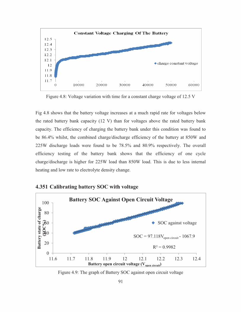
91
Figure 4.8: Voltage variation with time for a constant charge voltage of 12.5 V
Fig 4.8 shows that the battery voltage increases at a much rapid rate for voltages below
the rated battery bank capacity (12 V) than for voltages above the rated battery bank
capacity. The efficiency of charging the battery bank under this condition was found to
be 86.4% whilst, the combined charge/discharge efficiency of the battery at 850W and
225W discharge loads were found to be 78.5% and 80.9% respectively. The overall
efficiency testing of the battery bank shows that the efficiency of one cycle
charge/discharge is higher for 225W load than 850W load. This is due to less internal
heating and low rate to electrolyte density change.
4.351 Calibrating battery SOC with voltage
Figure 4.9: The graph of Battery SOC against open circuit voltage
SOC = 97.118Vopen circuit - 1067.9
R² = 0.9982 0
20
40
60
80
100
11.6 11.7 11.8 11.9 12 12.1 12.2 12.3 12.4
Bat
tery
stat
e of
cha
rge
(SO
C%
)
Battery open circuit voltage (Vopen circuit)
Battery SOC Against Open Circuit Voltage
SOC against voltage

92
The current conductance method (Coulomb counting) was used to determine the variation
of battery voltage with SOC for a discharge load of 850 W at a ambient temperature of
20-25oC. A linear relation between the open circuit voltage and SOC was observed as
shown in fig 4.9. The following mathematical relationships and regressions were
observed between the SOC and Vopen circuit for the AGM battery. 1067.9 - V 97.118 = % SOC circuitopen )( (4.11)
R2 = 0.9982.
The experimental results show a high degree of correlation between SOC and Vopen circuit.
Furthermore the SOC variation with Vopen circuit agrees well with the studies by Hammel et
al [156]. They found that the SOC varied linearly with open circuit voltage for valve
regulated lead acid battery (VRLA) according to equation 4.12.
965 - V 500 =(%) SOC circuitopen (4.12)
The SOC variation with Vopen circuit curve was used to determine the SOC of the laptop
charging battery from the measured values of open circuit voltage. However, Eq 4.11 can
only be applied to determine the battery state of charge when the battery is not being
charged since the charger applies a higher voltage than the actual battery voltage. The
current conductance method of battery charge determination in such a case provides the
most convenient method of determining SOC. Eq 4.11 can still be used to determine the
SOC provided that the mode of operation of the charge controller is known. If the charge
controller is operating in the bulk mode then equation 4.13 can be used to determine the
SOC.
1000.782 - V 96.728 =(%) SOC battery-controller charge (4.13)
Where,
battery-controller chargeV is the charge controller output voltage.
In bulk mode of charge controller operation, the battery is charged at 1V above the actual
battery bank voltage and as the voltage of the battery increases during charging, so does
the controller charging voltage and a difference of 1 volt is maintained between the actual
battery voltage and the charge controller voltage. If the charge controller is operating in
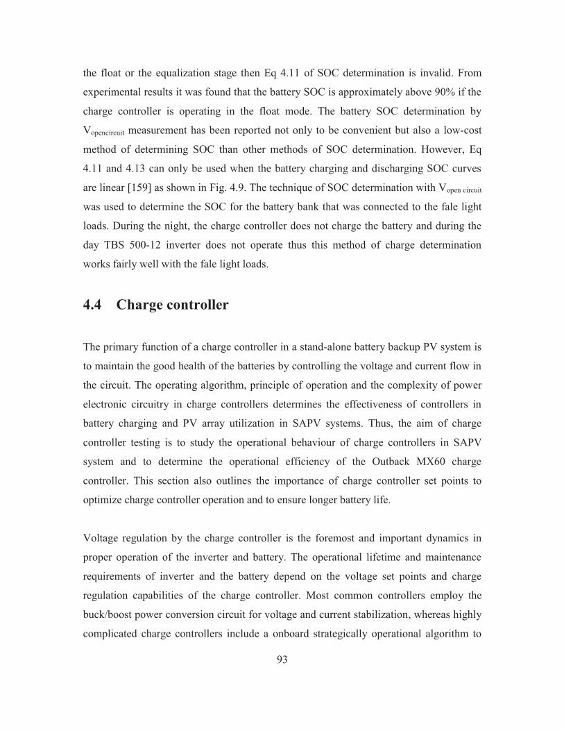
93
the float or the equalization stage then Eq 4.11 of SOC determination is invalid. From
experimental results it was found that the battery SOC is approximately above 90% if the
charge controller is operating in the float mode. The battery SOC determination by
Vopencircuit measurement has been reported not only to be convenient but also a low-cost
method of determining SOC than other methods of SOC determination. However, Eq
4.11 and 4.13 can only be used when the battery charging and discharging SOC curves
are linear [159] as shown in Fig. 4.9. The technique of SOC determination with Vopen circuit
was used to determine the SOC for the battery bank that was connected to the fale light
loads. During the night, the charge controller does not charge the battery and during the
day TBS 500-12 inverter does not operate thus this method of charge determination
works fairly well with the fale light loads.
4.4 Charge controller
The primary function of a charge controller in a stand-alone battery backup PV system is
to maintain the good health of the batteries by controlling the voltage and current flow in
the circuit. The operating algorithm, principle of operation and the complexity of power
electronic circuitry in charge controllers determines the effectiveness of controllers in
battery charging and PV array utilization in SAPV systems. Thus, the aim of charge
controller testing is to study the operational behaviour of charge controllers in SAPV
system and to determine the operational efficiency of the Outback MX60 charge
controller. This section also outlines the importance of charge controller set points to
optimize charge controller operation and to ensure longer battery life.
Voltage regulation by the charge controller is the foremost and important dynamics in
proper operation of the inverter and battery. The operational lifetime and maintenance
requirements of inverter and the battery depend on the voltage set points and charge
regulation capabilities of the charge controller. Most common controllers employ the
buck/boost power conversion circuit for voltage and current stabilization, whereas highly
complicated charge controllers include a onboard strategically operational algorithm to
94
monitor the battery status of charge, voltage, current, temperature, specific gravity and
efficiency of charging discharging. The later controllers also have built in algorithmically
intelligent control system to automatically diagnose or troubleshoot controller problems.
Strategic battery charging systems prevent the battery from over-charging and gassing
which are most common problem encountered in batteries. The built in intelligence in a
control system prolongs the battery life.
The correct operation of the charge controller is very essential in efficient operation of a
PV system and its components. Furthermore, it has been reported that the batteries in
SAPV systems are more often damaged by bad charging technique than by any other
cause [160]. Therefore, this chapter proposes to combines the algorithmic control
capabilities of Outback controller with results of battery and charge controller testing to
outline a efficient battery charging scheme for AGM battery.
4.41 Testing procedure
There are various standards available at international level for the validation and correct
operation of charge controllers in SAPV systems. The most commonly used standard of
charge controller testing are EN 50314-1 and EN 50314-2 [161]. European standards of
EN50081-1, EN50082-1, EN50081-2, EN 55011, EN55014, IEC 801-2, IEC 801-3,
IEC801-4 and EN 61000-4-2 are also used in performance evaluation of charge
controllers with respect to electrostatic discharge and overvoltage protection [162].
In this study, the Outback MX60 charge controller with MPPT was tested for dc-to-dc
conversion efficiency and MPPT operation under different mode of operation. The
controller specifications are given in table 4.6.

95
4.42 Outback MX60 Charge Controller
The Outback MX60 charge controller is a multi-stage, sophisticated battery charger that
uses several voltage regulation set points to allow fast recharging of the battery, while
ensuring a longer battery life. The charge controller has voltage set points for different
modes (absorb, float and equalization), which have to be edited accordingly to the battery
and inverter manufactures recommendations and PV system design.
The Outback battery charger consists of 7 major battery charging modes operating at 2
different maximum power point tracking method. The battery charging schemes consists
of snooze, wake-up, bulk, absorption, float, silent and equalization modes. The Outback
charge controller mode of operation changes during the day depending on the battery
state of charge, PV array output, and design of the whole system. Technical specifications
for Outback MX60charge controller are given in table 4.6.
The charge controller starts operation in the snooze mode. In this mode of operation the
controller measures the ISC (< 0.6A) to initiate the wake- up mode. In the wake-up mode
the controller performs the first track of the MPP and waits until the input power from the
modules is greater than 25W before it switches on to the absorption mode of operation.
The charge controller operates in the absorption mode if the battery voltage is below the
absorption set point voltage (12V). In this mode of operation, the voltage is held constant
for a specified time (default: 2hours) while charge controller limits the current going into
the battery. Furthermore, if the battery voltage is still below the absorption point voltage
a bulk cycle is reinitiated. The bulk cycle mode of operation delivers the maximum
power to the battery while slightly increasing the recharging voltage consecutively until
the battery voltage reaches the absorption set point voltage. The two modes of MPPT
operation are auto track MPPT or the U-Pick % (Voc) MPPT. The mode of MPPT
tracking used in this study is discussed in more detailed in section 4.5.

96
The float cycle follows after the absorption cycle is completed but if the charge controller
voltage falls below the float point voltage for a time interval of 90 seconds, the rebulk
mode is initiated and the charge controller operates to bulk the battery for the second
time. The charge controller will not re-initiate another bulk cycle if the float voltage set
point is not reached during the set time interval but, will continue to charge the battery
until the battery voltage reaches the float voltage. In addition, if the system cannot
maintain the float voltage set point, the charge controller will switch to the MPPT float
mode and try to regulate the batteries to the float voltage set point.
The cell equalization is the last and the foremost important process in determining the
proper operation of the battery. The importance of cell equalization is clarified in [163-
164]. In literature it has been reported that cells connected in series are subjected to
failures by charge imbalance effect, if the batteries are not equalized [165-167]. The
battery equalization process consists of overcharging the battery at a higher voltage than
the battery voltage for a short time to bring all the cells of the battery bank to the same
voltage. On the other hand, studies have also shown that the higher equalization voltage
works at the expense of gassing and causes electrolytic cell break down in batteries [170].
Whilst, it is also known that low equalization voltage set points does not optimally
regulate all the cells in a battery bank to the same state of charge. Therefore, the charge
controller set points have to be carefully chosen to attain optimized and efficient
performance from SAPV system. Lastly the charge controller goes in to the sleep mode
of operation if the ISC is less than 0.6A.
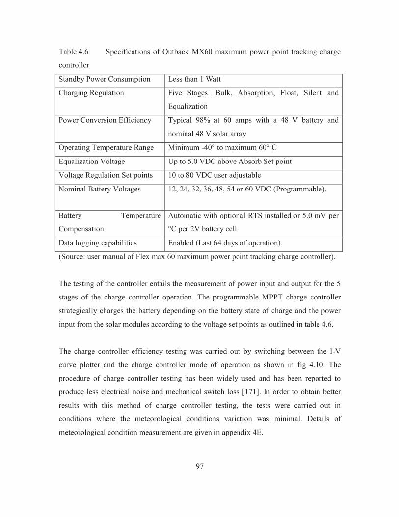
97
Table 4.6 Specifications of Outback MX60 maximum power point tracking charge
controller
Standby Power Consumption Less than 1 Watt
Charging Regulation Five Stages: Bulk, Absorption, Float, Silent and
Equalization
Power Conversion Efficiency Typical 98% at 60 amps with a 48 V battery and
nominal 48 V solar array
Operating Temperature Range Minimum -40° to maximum 60° C
Equalization Voltage Up to 5.0 VDC above Absorb Set point
Voltage Regulation Set points 10 to 80 VDC user adjustable
Nominal Battery Voltages 12, 24, 32, 36, 48, 54 or 60 VDC (Programmable).
Battery Temperature
Compensation
Automatic with optional RTS installed or 5.0 mV per
°C per 2V battery cell.
Data logging capabilities Enabled (Last 64 days of operation).
(Source: user manual of Flex max 60 maximum power point tracking charge controller).
The testing of the controller entails the measurement of power input and output for the 5
stages of the charge controller operation. The programmable MPPT charge controller
strategically charges the battery depending on the battery state of charge and the power
input from the solar modules according to the voltage set points as outlined in table 4.6.
The charge controller efficiency testing was carried out by switching between the I-V
curve plotter and the charge controller mode of operation as shown in fig 4.10. The
procedure of charge controller testing has been widely used and has been reported to
produce less electrical noise and mechanical switch loss [171]. In order to obtain better
results with this method of charge controller testing, the tests were carried out in
conditions where the meteorological conditions variation was minimal. Details of
meteorological condition measurement are given in appendix 4E.
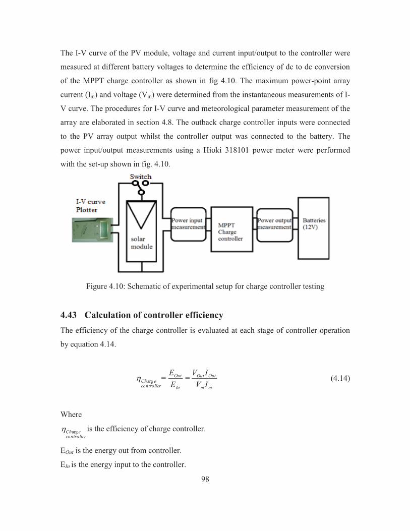
98
The I-V curve of the PV module, voltage and current input/output to the controller were
measured at different battery voltages to determine the efficiency of dc to dc conversion
of the MPPT charge controller as shown in fig 4.10. The maximum power-point array
current (Im) and voltage (Vm) were determined from the instantaneous measurements of I-
V curve. The procedures for I-V curve and meteorological parameter measurement of the
array are elaborated in section 4.8. The outback charge controller inputs were connected
to the PV array output whilst the controller output was connected to the battery. The
power input/output measurements using a Hioki 318101 power meter were performed
with the set-up shown in fig. 4.10.
Figure 4.10: Schematic of experimental setup for charge controller testing
4.43 Calculation of controller efficiency The efficiency of the charge controller is evaluated at each stage of controller operation
by equation 4.14.
mm
OutOut
In
Out
controllereCh IV
IV=
EE
=arg�
(4.14)
Where
controllereCharg� is the efficiency of charge controller.
EOut is the energy out from controller.
EIn is the energy input to the controller.
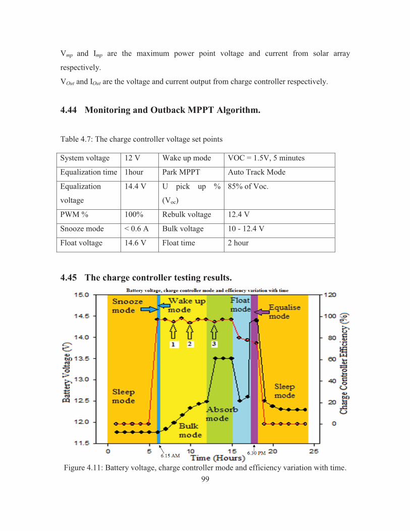
99
Vmp
and Imp are the maximum power point voltage and current from solar array
respectively.
VOut and IOut are the voltage and current output from charge controller respectively.
4.44 Monitoring and Outback MPPT Algorithm.
Table 4.7: The charge controller voltage set points
4.45 The charge controller testing results.
Figure 4.11: Battery voltage, charge controller mode and efficiency variation with time.
System voltage 12 V Wake up mode VOC = 1.5V, 5 minutes
Equalization time 1hour Park MPPT Auto Track Mode
Equalization
voltage
14.4 V U pick up %
(Voc)
85% of Voc.
PWM % 100% Rebulk voltage 12.4 V
Snooze mode < 0.6 A Bulk voltage 10 - 12.4 V
Float voltage 14.6 V Float time 2 hour
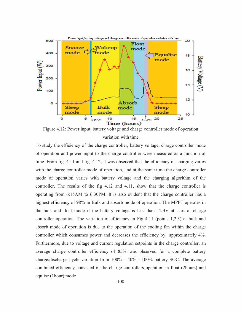
100
Figure 4.12: Power input, battery voltage and charge controller mode of operation
variation with time
To study the efficiency of the charge controller, battery voltage, charge controller mode
of operation and power input to the charge controller were measured as a function of
time. From fig. 4.11 and fig. 4.12, it was observed that the efficiency of charging varies
with the charge controller mode of operation, and at the same time the charge controller
mode of operation varies with battery voltage and the charging algorithm of the
controller. The results of the fig 4.12 and 4.11, show that the charge controller is
operating from 6:15AM to 6:30PM. It is also evident that the charge controller has a
highest efficiency of 98% in Bulk and absorb mode of operation. The MPPT operates in
the bulk and float mode if the battery voltage is less than 12.4V at start of charge
controller operation. The variation of efficiency in Fig 4.11 (points 1,2,3) at bulk and
absorb mode of operation is due to the operation of the cooling fan within the charge
controller which consumes power and decreases the efficiency by approximately 4%.
Furthermore, due to voltage and current regulation setpoints in the charge controller, an
average charge controller efficiency of 85% was observed for a complete battery
charge/discharge cycle variation from 100% - 40% - 100% battery SOC. The average
combined efficiency consisted of the charge controllers operation in float (2hours) and
equlise (1hour) mode.
101
4.5 Solar PV Module
In designing any renewable energy system that incorporates PV modules, there is a vital
requirement to accurately assess the output from the proposed PV array under various
operating conditions. PV modules are rating at Standard Test Conditions (STC) of 1000
Wm-2 solar irradiance incident normal to the module under Air Mass (AM) of 1.5 and a
cell temperature (inside the module) of 25°C [172].
Solar module specification data from manufacturers provide performance parameters at a
Standard Reporting Condition (SRC) defined by the ASTM [172]. The SRC provides a
reference condition for testing and reporting module performance. Models utilise SRC
performance data to derive module performance for all other operating conditions. Two
AM 1.5 solar spectra have been standardized by ASTM, one for concentrator modules
and the other for testing flat-plate modules [172]. In addition, internationally recognized
calibration standards have been established in an attempt to regulate worldwide
consistency in module performance measurement [173]. The test results of Carr A. J
[174] show that the STC values quoted by PV modules manufacturers data sheet for their
modules under STC conditions do not necessarily match those with test conducted in
outdoor STC measurements. In recent years, the over rating issue has been minimized
due to the adoption of EN 5380 standard in Europe and UL4730 standard in the United
States, however it has not been completely eliminated as of now.
Studies by Chowdhurya et al [175] on charge controller MPP tracking algorithm using
field programmable gate method and solar array I-V curve have shown better results in-
terms of time response and efficiency when compared to the existing basic Perturb and
Observe method (P&O). The Outback charge controller used in the design of SAPV
system has two methods of tracking the MPP. The first method is based on MPP tracking
on P-V characteristic curve of the array. For the first method of MPP the charge
controller at the start of the charge controller operation determines the MPP from
102
tracking I-V curve. The second method is based on the Voc measurement of the solar
array by the charge controller. In this method open circuit voltage method needs the user
to set the percentage of Voc the MPP is located and the MPPT tracks the MPP by
measuring the Voc. The percentage of Voc the MPP is can be determined by the P-V of the
array. This section deals with determining the I-V & P-V curve, temperature coefficients
of voltage, current and power for the solar modules under outdoor conditions. The Sandia
model of solar module testing was used to evaluate the performance of the modules under
outdoor conditions. The results of this section are later used in solar cell modelling in PV
design Pro™, PVsyst™ and HOMER™ Software. These results are also used to select
the MPP mode (park MPPT or Upickup) of operation in Outback MX60TM charge
controller.
4.51 Standards of solar module Testing
The American society for testing and materials (ASTM) standard for testing and
reporting performance of solar modules based on I-V characteristic curve is the most
widely used standard in evaluating the performance of solar modules [172]. The most
used models in the world are based on the ASTM E 1036 and IEC 60904 standards. They
are continuously validated by several research and testing groups around the world.
The Sandia performance model coupled with parameters from the module database
provides a well-established alternative that has been verified to work well for all
commercially available module and array technologies [176]. The purpose of this testing
was to empirically derive performance estimates from PV modules under a variety of
operating conditions. In addition to the ASTM standard, there are World Photovoltaic
Scale (WPVS), IEC and other standards that are also used to evaluate the performance of
flat plate PV modules [177]. The ASTM E973, ASTM E 1036-02, ASTM E 1362 and
Sandia performance model are well established models used in assessing the performance
of PV modules [174]. Studies have shown that the Sandia model can be used to evaluate
to access the performance of both module and arrays [174].
103
The purpose of this section is to study the PV module’s performance under outdoor
operating conditions. The parameters studied are temperature, radiation and partial
shading of the modules. The basic equations used in determining the performance of the
module and the array are listed in the appendix 4F.
4.52 Sandia Module Performance Model
The Sandia module performance model has been developed at the Sandia National
Laboratories and is based on experimental observation and the equations used in the
models are derived from the individual solar cell characteristics [178]. It is applicable in
evaluation of PV cells performance at module and array levels and has been successfully
used in designing and monitoring photovoltaic systems [179-182].
The Sandia module database contains experimentally derived modules performance
equations from different manufacturers. The outlined model has also been used in
software to model PV array and module performance [176]. In addition to the expressions
for the solar cell modeling, the Sandia model details I-V curve modeling by introducing
two extra points that better define the shape of the I-V curve and increase the accuracy of
I-V curve modeling.
The module I-V curve measurements were carried out at different temperatures and
radiation to determine the efficiency of the modules at 800W/m2 irradiance. The details of
radiation, temperature, wind speed, data measuring algorithm is given in Appendix 4G.
104
4.53 Module Testing Procedure
4.531 Part 1 : I-V curve of Conergy solar panels.
The variation of open circuit voltage (Voc), maximum power point voltage (Vmp) and
MPP with radiation was studied for the Conergy solar panels. The I-V curves were
measured with a PVK mini I-V curve tracer at 11 AM for a horizontally oriented
Conergy PV module. The specification of the PVK mini I-V curve tracer and Conergy
PV module are given in appendix 4H and 4I respectively.
The characteristic I-V curve of Conergy PV modules were measured at constant
temperature of 25 ± 2oC at different irradiances. The study of PV module performance
variation with radiation was carried out by measuring I-V curves at constant irradiance of
500Wm-2 ± 5%. The back-of-module temperature readings were used to determine the
PV module cell temperature [174]. Solar radiation and other meteorological conditions
such as wind-speed, wind direction, humidity and ambient temperature were also
measured. The details of meteorological parameter measurements, instruments
specifications and data recording system are provided in Appendix 4G and 4E.
The analysis of the I-V curve was used to select the mode of MPPT operation for the
charge controller. The configuration and mode of operation of the charge controller are
discussed in more detail in section 4.42.
4.532 Temperature Coefficients
A similar procedure for measuring the I-V curve as in section 4.531 was also used in
section 4.532. The coefficient of temperature variation with Isc, Voc and Pmp was
determined from the I-V curves of the module at different module temperatures ranging
from 20-60oC and constant irradiance of 800 ± 10 Wm-2. The measurements were
performed at 11 AM using the Mini I-V curve plotter. From the plot of Isc, Voc and Pmp
105
variation with temperature, the coefficient of Isc, Voc and Pmp variation were determined.
The temperature coefficients were obtained by firstly performing linear regression on test
data and then determining the gradient of the respective curves. The results of this
analysis shown in Fig 4.14. Other meteorological conditions that were also measured in
this test were the wind-speed, and ambient temperature. The details of meteorological
condition instruments specifications, measurements and data recording system are
provided in appendix 4E.
4.54 The effect of shading on power output
The module I-V curves were plotted using the PVK mini I-V curve plotter under different
shading patterns. The pattern of module shading was determined by the simulation results
and daily observation of shade on the module at the site of installation. The I-V curves
were analysed to study the effect of shading on module performance. The shading at
array level was obtained by adding the I-V curves of the individual modules under
different shading conditions.
4.55 Results of solar PV module Testing
4.551 I-V curves of Conergy solar modules.
Fig 4.13 delineates that the power output of the Conergy modules varies rapidly with
radiation. It also shows that the short circuit current (Isc) output of the Conergy modules
has a greater variation with radiation as compared to that of open circuit voltage (Voc).
From Fig 4.14 it is observed that the Isc variation with temperature has a direct
relationship whilst Voc variation with temperature have an inverse relationship. The study
of Voc and Isc variation with temperature correlates well with studies by Carr [174]. Their
studies show that the modules become less efficient as the temperature increases. The
effect of increasing temperature on Conergy solar module also decreases the yield of the
module as delineated in Fig 4.14.
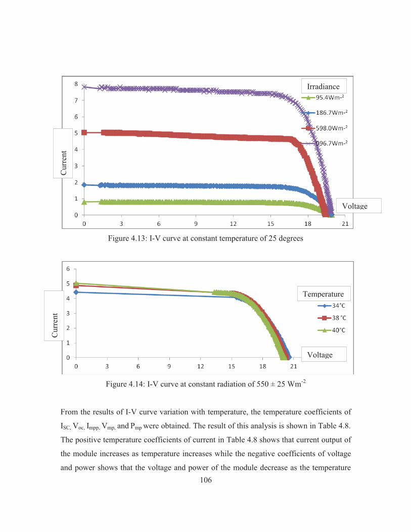
106
Figure 4.13: I-V curve at constant temperature of 25 degrees
Figure 4.14: I-V curve at constant radiation of 550 ± 25 Wm-2
From the results of I-V curve variation with temperature, the temperature coefficients of
ISC, Voc, Impp, Vmp, and Pmp were obtained. The result of this analysis is shown in Table 4.8.
The positive temperature coefficients of current in Table 4.8 shows that current output of
the module increases as temperature increases while the negative coefficients of voltage
and power shows that the voltage and power of the module decrease as the temperature
Irradiance
Temperature
Voltage
Cur
rent
Voltage
Cur
rent
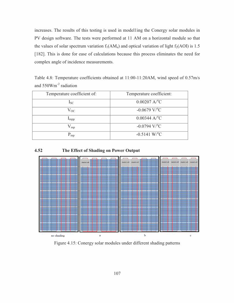
107
increases. The results of this testing is used in model1ing the Conergy solar modules in
PV design software. The tests were performed at 11 AM on a horizontal module so that
the values of solar spectrum variation f1(AMa) and optical variation of light f2(AOI) is 1.5
[182]. This is done for ease of calculations because this process eliminates the need for
complex angle of incidence measurements.
Table 4.8: Temperature coefficients obtained at 11:00-11:20AM, wind speed of 0.57m/s
and 550Wm-2 radiation
Temperature coefficient of: Temperature coefficient:
ISC 0.00207 A/oC
VOC -0.0679 V/oC
Impp 0.00344 A/oC
Vmp -0.0794 V/oC
Pmp -0.5141 W/oC
4.52 The Effect of Shading on Power Output
Figure 4.15: Conergy solar modules under different shading patterns
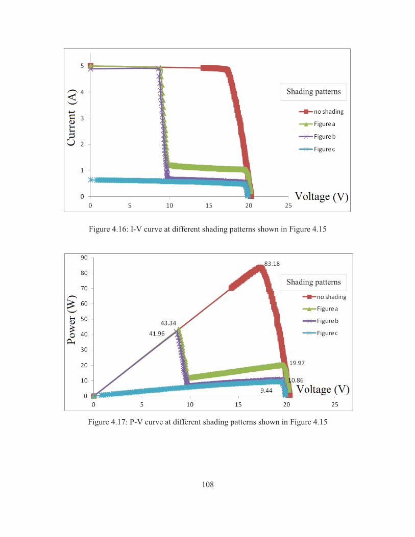
108
Figure 4.16: I-V curve at different shading patterns shown in Figure 4.15
Figure 4.17: P-V curve at different shading patterns shown in Figure 4.15
Shading patterns
Shading patterns
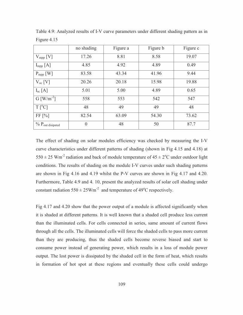
109
Table 4.9: Analyzed results of I-V curve parameters under different shading pattern as in
Figure 4.15
no shading Figure a Figure b Figure c
Vmpp [V] 17.26 8.81 8.58 19.07
Impp [A] 4.85 4.92 4.89 0.49
Pmpp [W] 83.58 43.34 41.96 9.44
Voc [V] 20.26 20.18 15.98 19.88
Isc [A] 5.01 5.00 4.89 0.65
G [W/m-2] 558 553 542 547
T [oC] 48 49 49 48
FF [%] 82.54 63.09 54.30 73.62
% Pout disipated 0 48 50 87.7
The effect of shading on solar modules efficiency was checked by measuring the I-V
curve characteristics under different patterns of shading (shown in Fig 4.15 and 4.18) at
550 ± 25 Wm-2 radiation and back of module temperature of 45 ± 2oC under outdoor light
conditions. The results of shading on the module I-V curves under such shading patterns
are shown in Fig 4.16 and 4.19 whilst the P-V curves are shown in Fig 4.17 and 4.20.
Furthermore, Table 4.9 and 4. 10, present the analyzed results of solar cell shading under
constant radiation 550 ± 25Wm-2 and temperature of 49oC respectively.
Fig 4.17 and 4.20 show that the power output of a module is affected significantly when
it is shaded at different patterns. It is well known that a shaded cell produce less current
than the illuminated cells. For cells connected in series, same amount of current flows
through all the cells. The illuminated cells will force the shaded cells to pass more current
than they are producing, thus the shaded cells become reverse biased and start to
consume power instead of generating power, which results in a loss of module power
output. The lost power is dissipated by the shaded cell in the form of heat, which results
in formation of hot spot at these regions and eventually these cells could undergo

110
permanent breakdown. If the sum of voltages of un-shaded cell exceeds the diode reverse
breakdown voltage, an irreversible damage occurs to the cell [183].
Results in table 4.9 shows that 48%, 50% and 88.7% of the power is dissipated by the
cells under respective shading patterns in Fig 4.15. Whilst the results of Table 4.10 show
that 48%, 50% and 45% of the power is dissipated under the shading pattern outlined in
Fig 4.18. Fig 4.15 has 4 cells shaded and the power output decreases by 88.7% whilst Fig
4.18 c has 18 cells shaded and the power output decreases by 44.9%. Comparing results
of shading pattern in Fig 4.15 c and Fig 4.18 c, it is clearly shown that the shading pattern
and diode arrangement has a significant impact on power output of the module. In Fig
4.15 c, the two strings have the same pattern of shading, thus the voltage and current
output is same from each string and the I-V curve does not have two local maximum
power points. The presence of shaded cells in each string consumes most of the generated
power in each string thus the module power output decreases significantly. In Fig 4.18 c
one whole string is shaded while the other string is not, thus the voltage and current from
the illuminated string contributes to the power output of the module, the bypass diodes
across the shaded string limits the current flow through the shaded cells.
The P-V curves in Fig 4.17 a, b and 4.20 a, b show that due to shading there are two local
maxima for MPP. Fig 4.17 c has one maxima than the usual two as in Fig 4.17 a, b and
4.20 a, b. In Fig 4.17 c each of the 2 strings has 2 cells that are shaded, thus the power
output is same from each string and thus the I-V curve has one MPP. Fig 4.20 c shows
that the illuminated cell dominates the power output of the module and has one MPP for
the module. The Conergy solar modules have two strings with 18 cells in each string. Fig
4.16 a, b and 4.19 a, b have 1 and 2 cells shaded for 1 string with other sting being in full
illumination. The I-V curves below 10 V in Fig 4.16 a, b and 4.19 a, b shows the current
and voltage output from first string and above 10V for the second string. Thus the
combined result of shading of one string results in two MPP in a shaded cell.
Chowdhurya et al [175] reported that local maxima can confuse the maximum power
point tracking algorithm and lead the MPPT to track the lower power output local
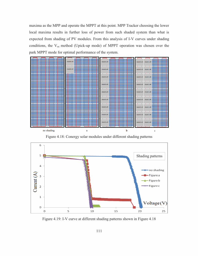
111
maxima as the MPP and operate the MPPT at this point. MPP Tracker choosing the lower
local maxima results in further loss of power from such shaded system than what is
expected from shading of PV modules. From this analysis of I-V curves under shading
conditions, the Voc method (Upick-up mode) of MPPT operation was chosen over the
park MPPT mode for optimal performance of the system.
Figure 4.18: Conergy solar modules under different shading patterns
Figure 4.19: I-V curve at different shading patterns shown in Figure 4.18
Shading patterns
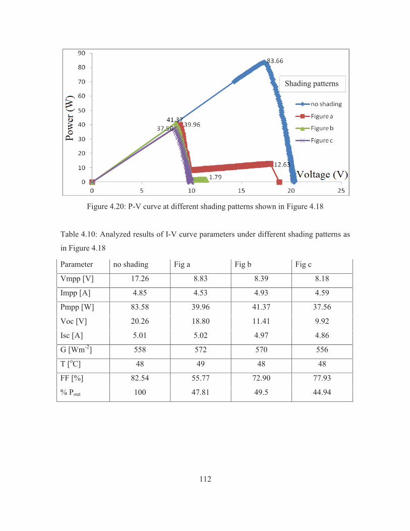
112
Figure 4.20: P-V curve at different shading patterns shown in Figure 4.18
Table 4.10: Analyzed results of I-V curve parameters under different shading patterns as
in Figure 4.18
Parameter no shading Fig a Fig b Fig c
Vmpp [V] 17.26 8.83 8.39 8.18
Impp [A] 4.85 4.53 4.93 4.59
Pmpp [W] 83.58 39.96 41.37 37.56
Voc [V] 20.26 18.80 11.41 9.92
Isc [A] 5.01 5.02 4.97 4.86
G [Wm-2] 558 572 570 556
T [oC] 48 49 48 48
FF [%] 82.54 55.77 72.90 77.93
% Pout 100 47.81 49.5 44.94
Shading patterns
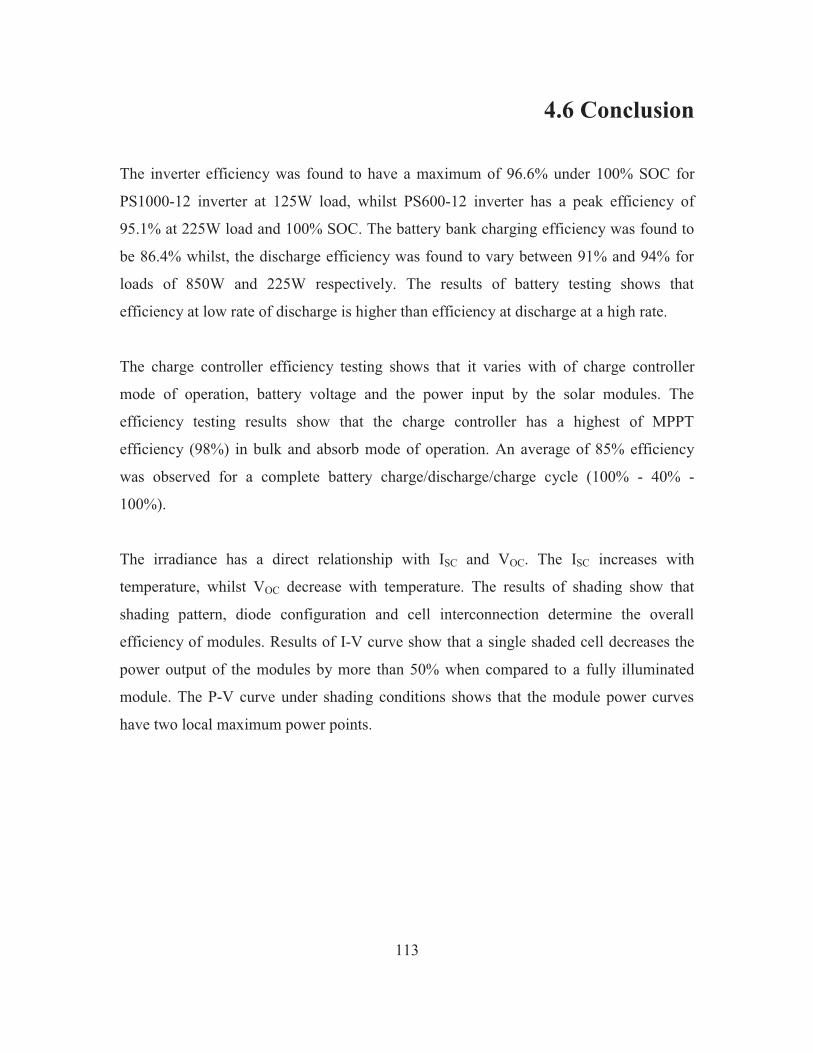
113
4.6 Conclusion
The inverter efficiency was found to have a maximum of 96.6% under 100% SOC for
PS1000-12 inverter at 125W load, whilst PS600-12 inverter has a peak efficiency of
95.1% at 225W load and 100% SOC. The battery bank charging efficiency was found to
be 86.4% whilst, the discharge efficiency was found to vary between 91% and 94% for
loads of 850W and 225W respectively. The results of battery testing shows that
efficiency at low rate of discharge is higher than efficiency at discharge at a high rate.
The charge controller efficiency testing shows that it varies with of charge controller
mode of operation, battery voltage and the power input by the solar modules. The
efficiency testing results show that the charge controller has a highest of MPPT
efficiency (98%) in bulk and absorb mode of operation. An average of 85% efficiency
was observed for a complete battery charge/discharge/charge cycle (100% - 40% -
100%).
The irradiance has a direct relationship with ISC and VOC. The ISC increases with
temperature, whilst VOC decrease with temperature. The results of shading show that
shading pattern, diode configuration and cell interconnection determine the overall
efficiency of modules. Results of I-V curve show that a single shaded cell decreases the
power output of the modules by more than 50% when compared to a fully illuminated
module. The P-V curve under shading conditions shows that the module power curves
have two local maximum power points.
114
Chapter 5 5.0 Design & Simulation
5.1 SAPV System Design & Simulation
Renewable energy design and simulation software packages are the most widely used
tools for designing and evaluating the performance of RE systems [184]. There are many
simulation software available for modelling, designing and simulating the performance of
PV systems based on different modelling complexities, requirements of the user, type of
system, software working platform and availability of simulation data.
In this work, PV systTM, HOMERTM and Solar Design StudioTM software are used to
design and simulate a 1.2kW standalone photovoltaic system for the USP student fales.
These software’s are also used to simulate the performance of the SAPV system. The
1.2kW PV system consisted of two independent subsystems for lights and laptop
charging respectively. The SAPV system is designed according to AS/NZS 4509
standard. The two systems are electrically isolated but are located at the same place and
under same environmental conditions. Each system consists of PV 5 modules, a charge
controller, battery and an inverter. The result of this analysis is used to design and
evaluate the performance of an optimum standalone system for the USP student fales.
The feasibility assessment and modelling of the SAPV system was conducted using
HOMER and the optimization results of this section were applied to determine the SAPV
system size and performance of the PV systems designed with the help of, PV systTM and
Solar Design StudioTM software. The PV system is simulated in, PV systTM to determine
the impact of shading on PV array performance, whilst a detailed economic analysis was
performed using the Solar Design StudioTM.
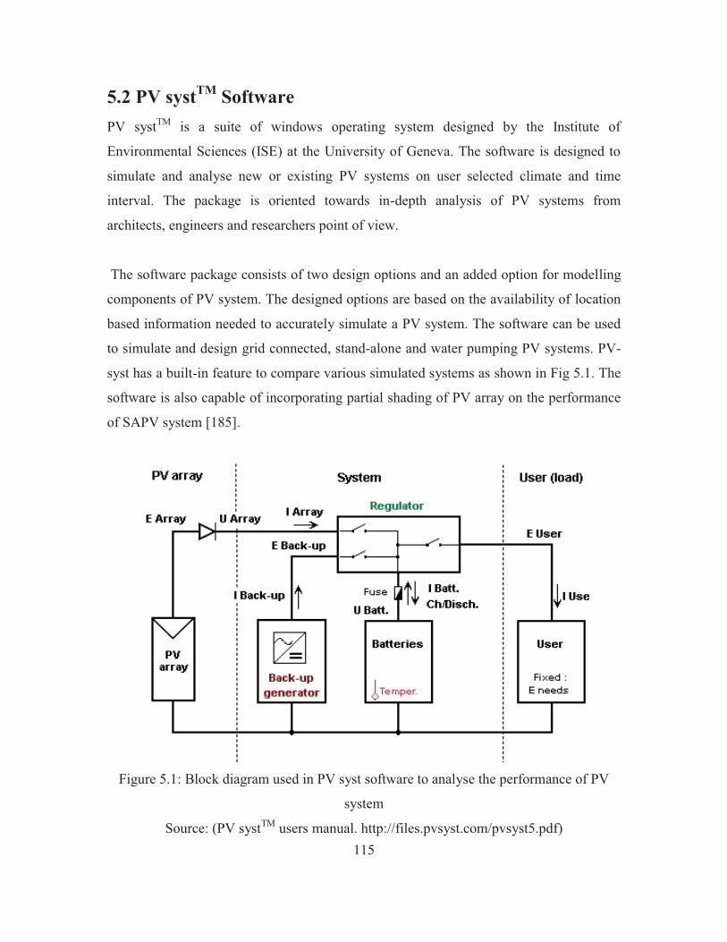
115
5.2 PV systTM Software PV systTM is a suite of windows operating system designed by the Institute of
Environmental Sciences (ISE) at the University of Geneva. The software is designed to
simulate and analyse new or existing PV systems on user selected climate and time
interval. The package is oriented towards in-depth analysis of PV systems from
architects, engineers and researchers point of view.
The software package consists of two design options and an added option for modelling
components of PV system. The designed options are based on the availability of location
based information needed to accurately simulate a PV system. The software can be used
to simulate and design grid connected, stand-alone and water pumping PV systems. PV-
syst has a built-in feature to compare various simulated systems as shown in Fig 5.1. The
software is also capable of incorporating partial shading of PV array on the performance
of SAPV system [185].
Figure 5.1: Block diagram used in PV syst software to analyse the performance of PV
system
Source: (PV systTM users manual. http://files.pvsyst.com/pvsyst5.pdf)
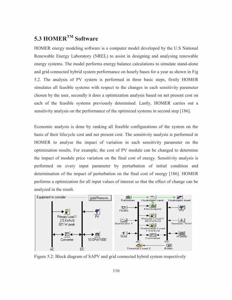
116
5.3 HOMERTM Software HOMER energy modeling software is a computer model developed by the U.S National
Renewable Energy Laboratory (NREL) to assist in designing and analysing renewable
energy systems. The model performs energy balance calculations to simulate stand-alone
and grid connected hybrid system performance on hourly bases for a year as shown in Fig
5.2. The analysis of PV system is performed in three basic steps, firstly HOMER
simulates all feasible systems with respect to the changes in each sensitivity parameter
chosen by the user, secondly it does a optimization analysis based on net present cost on
each of the feasible systems previously determined. Lastly, HOMER carries out a
sensitivity analysis on the performance of the optimized systems in second step [186].
Economic analysis is done by ranking all feasible configurations of the system on the
basis of their lifecycle cost and net present cost. The sensitivity analysis is performed in
HOMER to analyse the impact of variation in each sensitivity parameter on the
optimization results. For example, the cost of PV module can be changed to determine
the impact of module price variation on the final cost of energy. Sensitivity analysis is
performed on every input parameter by perturbation of initial condition and
determination of the impact of perturbation on the final cost of energy [186]. HOMER
performs a optimization for all input values of interest so that the effect of change can be
analyzed in the result.
Figure 5.2: Block diagram of SAPV and grid connected hybrid system respectively

117
5.4 Solar Design StudioTM Software
PV Design ProTM is a software package for designing, simulating and data analysis of a
PV based RE system. There are three versions of PV Design ProTM software namely "PV-
DesignPro-S", "PV-DesignPro-G" and "PV-DesignPro-P”. PV Design Pro-S is for stand-
alone PV system with battery storage, whilst PV Design Pro-G and PV Design Pro-P are
for grid connected PV system and water pumping systems respectively.
The PV Design ProTM software is aimed at designing and simulation of accurate and in-
depth performance of PV system power output and load consumption during the
operation of the system. The software also performs economical analysis and evaluates
the financial impacts of installing the proposed system.
5.5 Modelling
5.5.1 Solar Irradiance and Shading
HOMER uses the HDKR (Hay, Davies, Klucher, Reindl) model to calculate the global
radiation on the array plane. The software allows measured hourly, monthly and annual
average data radiation to be used in the simulation of PV system. The Graham and
Hollands algorithm is used to convert the monthly and annual radiation data to hourly
data [187].
Furthermore, HOMER divides the global radiation into beam and diffuse radiation. The
beam component of the global radiation has a strong dependence on the receiving plane
tilt and orientation. Thus HOMER uses the Erb’s [188] method to determine the beam
and the diffuse radiation. The beam and diffuse radiation is later used in the HDKR
model (Eq 5.1) to calculate the global radiation on the plane of the array.
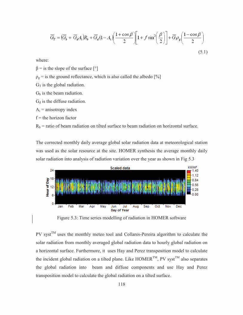
118
(5.1)
where:
β = is the slope of the surface [°]
ρg = is the ground reflectance, which is also called the albedo [%]
GT is the global radiation.
Gb is the beam radiation.
Gd is the diffuse radiation.
Ai = anisotropy index
f = the horizon factor
Rb = ratio of beam radiation on tilted surface to beam radiation on horizontal surface.
The corrected monthly daily average global solar radiation data at meteorological station
was used as the solar resource at the site. HOMER synthesis the average monthly daily
solar radiation into analysis of radiation variation over the year as shown in Fig 5.3
Figure 5.3: Time series modelling of radiation in HOMER software
PV systTM uses the monthly meteo tool and Collares-Pereira algorithm to calculate the
solar radiation from monthly averaged global radiation data to hourly global radiation on
a horizontal surface. Furthermore, it uses Hay and Perez transposition model to calculate
the incident global radiation on a tilted plane. Like HOMERTM, PV systTM also separates
the global radiation into beam and diffuse components and use Hay and Perez
transposition model to calculate the global radiation on a tilted surface.
119
Similar to HOMER and PV syst, Solar design studio uses HDKR and Perez model to
calculate global radiation on tilted plane. Furthermore, Solar Design Studio uses the 30
year averaged climate data from National Renewable Energy Laboratory to provide solar
insolation at the site to accurately simulate radiation on a horizontal surface. In this work,
the monthly corrected solar radiation data from section 3.5.1 in chapter 3 was used as
solar resource input in PV-syst software, whilst the solar access measurement at the site
was also ingested in PV-syst to make necessary corrections in solar resource caused by
shading of trees and buildings.
5.5.2 Shading
HOMER does not have a shade analysis tool incorporated in the software model unlike
in PV syst and the Solar Design Studio software. The effect of shading on array output in
HOMER was done by adjusting the PV derating factor. A derating factor of 85% was
used to account for partial shading of the PV array.
The PVsyst software uses a complex two step analysis method to analyse shading on PV
array. The two step shade analysis method looks at both far and near shadings. The
fundamental difference between the two types of shadings is that far shadings are due to
horizon effects that obstruct the global radiation on the PV field (eg mountains), whilst
near shading effects are those that obstruct the beam radiation on the PV modules (eg
shading due to nearby buildings and trees).
The far shading effects at the site of installation were determined from the Sun Eye 210
instrument with the method outlined in section 2.3.2. Fig 5.4 shows the far shading
effects modeling used in PV systTM software. Near shading assessment requires modeling
of building and trees near the location and its environment. The tree heights and distance
from the site of installation was measured with a Global Positioning System (GPS). The
University of South Pacific (USP) plan was used to construct the near shading diagram as
shown in Fig 5.5.
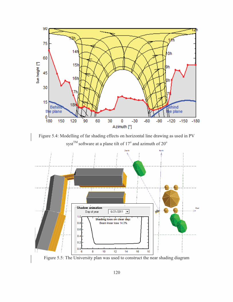
120
Figure 5.4: Modelling of far shading effects on horizontal line drawing as used in PV
systTM software at a plane tilt of 17o and azimuth of 20o
Figure 5.5: The University plan was used to construct the near shading diagram
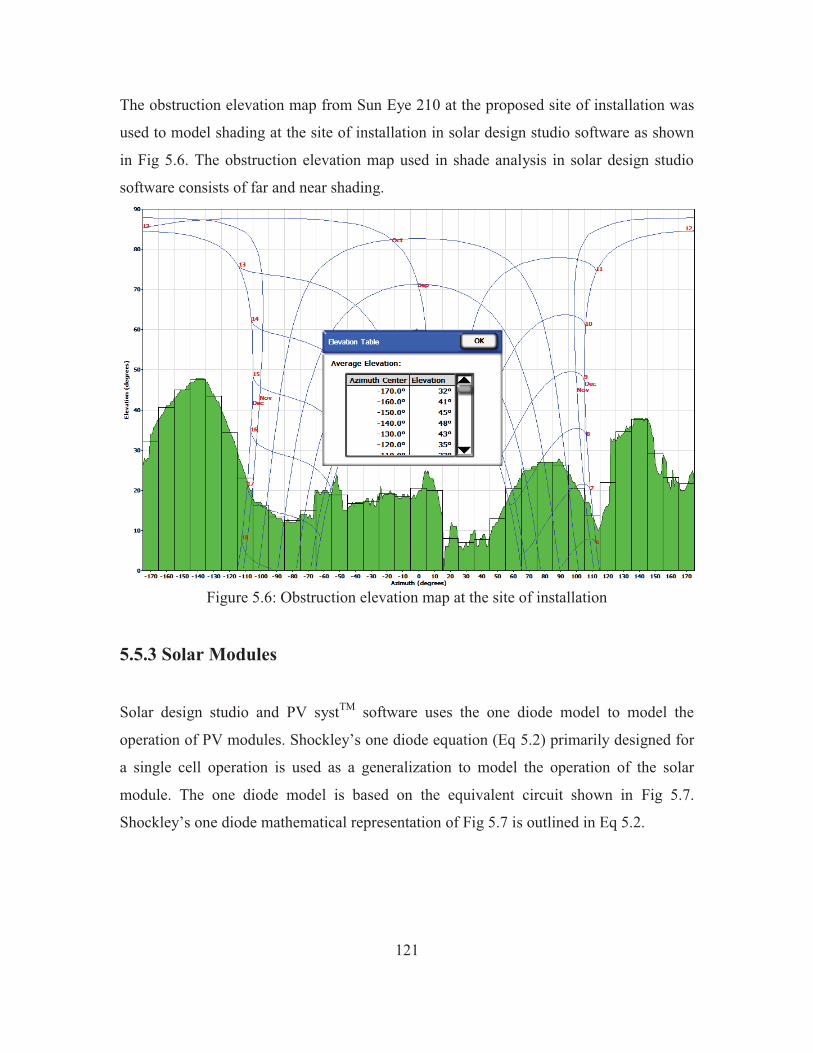
121
The obstruction elevation map from Sun Eye 210 at the proposed site of installation was
used to model shading at the site of installation in solar design studio software as shown
in Fig 5.6. The obstruction elevation map used in shade analysis in solar design studio
software consists of far and near shading.
Figure 5.6: Obstruction elevation map at the site of installation
5.5.3 Solar Modules
Solar design studio and PV systTM software uses the one diode model to model the
operation of PV modules. Shockley’s one diode equation (Eq 5.2) primarily designed for
a single cell operation is used as a generalization to model the operation of the solar
module. The one diode model is based on the equivalent circuit shown in Fig 5.7.
Shockley’s one diode mathematical representation of Fig 5.7 is outlined in Eq 5.2.
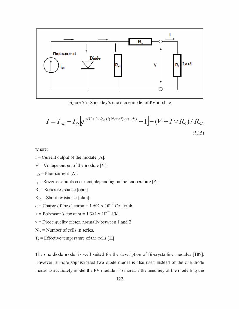
122
Figure 5.7: Shockley’s one diode model of PV module
� � ShSkTNcsRIVq
Oph RRIVeIII CS /)(1)/()( ������ �����
(5.15)
where:
I = Current output of the module [A].
V = Voltage output of the module [V].
Iph = Photocurrent [A].
Io = Reverse saturation current, depending on the temperature [A].
Rs = Series resistance [ohm].
Rsh = Shunt resistance [ohm].
q = Charge of the electron = 1.602 x 10⁻¹⁹ Coulomb
k = Bolzmann's constant = 1.381 x 10⁻²³ J/K.
γ = Diode quality factor, normally between 1 and 2
Ncs = Number of cells in series.
Tc = Effective temperature of the cells [K]
The one diode model is well suited for the description of Si-crystalline modules [189].
However, a more sophisticated two diode model is also used instead of the one diode
model to accurately model the PV module. To increase the accuracy of the modelling the
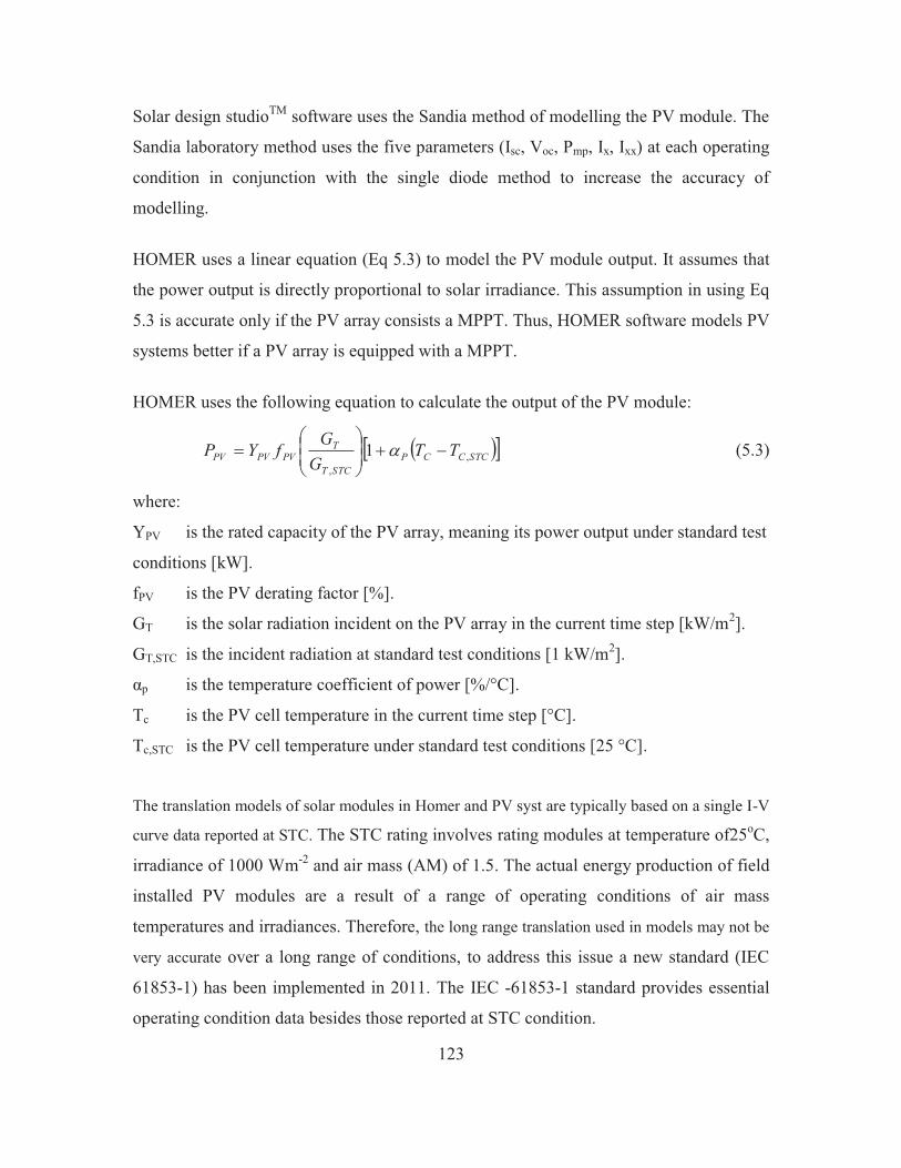
123
Solar design studioTM software uses the Sandia method of modelling the PV module. The
Sandia laboratory method uses the five parameters (Isc, Voc, Pmp, Ix, Ixx) at each operating
condition in conjunction with the single diode method to increase the accuracy of
modelling.
HOMER uses a linear equation (Eq 5.3) to model the PV module output. It assumes that
the power output is directly proportional to solar irradiance. This assumption in using Eq
5.3 is accurate only if the PV array consists a MPPT. Thus, HOMER software models PV
systems better if a PV array is equipped with a MPPT.
HOMER uses the following equation to calculate the output of the PV module:
�� �STCCCPSTCT
TPVPVPV TT
GGfYP ,
,
1 ����
����
�� �
(5.3)
where:
YPV is the rated capacity of the PV array, meaning its power output under standard test
conditions [kW].
fPV is the PV derating factor [%]. GT is the solar radiation incident on the PV array in the current time step [kW/m2]. GT,STC is the incident radiation at standard test conditions [1 kW/m2]. αp is the temperature coefficient of power [%/°C]. Tc is the PV cell temperature in the current time step [°C]. Tc,STC is the PV cell temperature under standard test conditions [25 °C].
The translation models of solar modules in Homer and PV syst are typically based on a single I-V
curve data reported at STC. The STC rating involves rating modules at temperature of25oC,
irradiance of 1000 Wm-2 and air mass (AM) of 1.5. The actual energy production of field
installed PV modules are a result of a range of operating conditions of air mass
temperatures and irradiances. Therefore, the long range translation used in models may not be
very accurate over a long range of conditions, to address this issue a new standard (IEC
61853-1) has been implemented in 2011. The IEC -61853-1 standard provides essential
operating condition data besides those reported at STC condition.
124
5.5.4 Inverter HOMERTM uses a three step efficiency method to mathematically model inverters. In
HOMER software the inverter is modeled as a converter which has a combined task of an
inverter and a rectifier. The software calculates the overall efficiency of the converter by
multiplying the efficiency of the rectifier and the inverter.
In PV syst the inverter is part of the regulator whilst in Solar Design Studio the inverter is
a separate component. The simulation in PV syst and solar design studio software
requires detailed information of inverter operating voltages and performance
parameterization setpoints. PV syst and Solar Design Studio both use the load against
efficiency curve (Fig 4.3) to determine the time series operation of inverter with load.
The inverter efficiency and voltage setpoints were included in the software using the data
from manufactures’ specification manuals and our results of inverter testing from section
4.34.
5.5.5 Charge Controller HOMER and Solar design studio software do not model the charge controller as a
separate component like PV systTM. The charge controller in HOMER and PV syst
software was modeled as part of the PV array. The PV module and charge controller cost
and efficiency were communally modeled in the software as part of the PV array. In
HOMER, an array derating factor of 0.98 was used to account for the controller
efficiency, whilst in solar design studio the PV MPPT device efficiency of 98% was used.
The charge controller in PV syst software is part of the regulator. The charge controller
operation and parameterization are similar to the inverter. The simulation process
requires detailed specific energy loss parameterization operating setpoints of efficiency,
power overloads thresholds of voltage and current of the controller. The charge controller
modeling consisted of voltage setpoint as in table 4.7 and the results of charge controller
testing together with the manufactures specification data which has been outlined in
section 4.4.
125
5.5.6 Battery The Kinetic Battery Model is used by HOMER software to determine the amount of
energy that can be withdrawn from or absorbed by a battery bank at each time step of
simulation. HOMER uses the two additional equations of energy balance within the
battery to calculate the charge and discharge energy at the beginning and end of each
time step of simulation. The two equations of energy give the allowable range for power
to flow into or out of the battery bank in any one-time step of simulation.
PV syst uses two-level phenomenological classical Shepherd's model to perform a
detailed analysis of battery performance. Two-level phenomenological non conventional
battery model uses the voltage with respect to the state of charge (SOC), internal
resistance and the temperature to describe the battery performance.
The battery model in solar design studio is that of a lead acid battery as elaborated in
“Handbook of batteries”, [190]. The model in solar design studio does not account for
temperature effects on battery performance. The result of battery testing in section 4.35
and the manufactures specification manual were used to model the TUDOR battery in the
three software’s.
5.5.7 Load Light and laptop charging load simulation was carried out using the above three software.
The light load consisted of 10 lights of 25W each. While the laptop load consisted of 4
laptops of 60W each, operating only during the day. All the three software use hourly
values of load in simulation. The hourly light and laptop load modelling used in the three
software is shown in Fig 5.8.
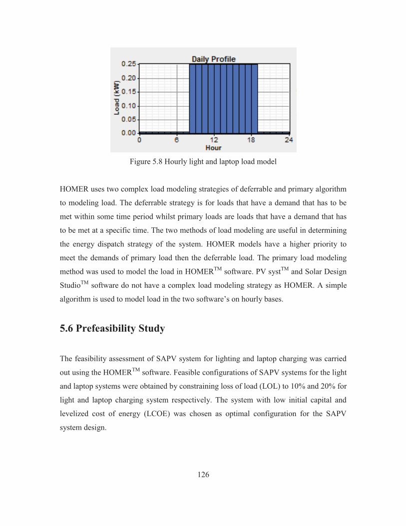
126
Figure 5.8 Hourly light and laptop load model
HOMER uses two complex load modeling strategies of deferrable and primary algorithm
to modeling load. The deferrable strategy is for loads that have a demand that has to be
met within some time period whilst primary loads are loads that have a demand that has
to be met at a specific time. The two methods of load modeling are useful in determining
the energy dispatch strategy of the system. HOMER models have a higher priority to
meet the demands of primary load then the deferrable load. The primary load modeling
method was used to model the load in HOMERTM software. PV systTM and Solar Design
StudioTM software do not have a complex load modeling strategy as HOMER. A simple
algorithm is used to model load in the two software’s on hourly bases.
5.6 Prefeasibility Study
The feasibility assessment of SAPV system for lighting and laptop charging was carried
out using the HOMERTM software. Feasible configurations of SAPV systems for the light
and laptop systems were obtained by constraining loss of load (LOL) to 10% and 20% for
light and laptop charging system respectively. The system with low initial capital and
levelized cost of energy (LCOE) was chosen as optimal configuration for the SAPV
system design.
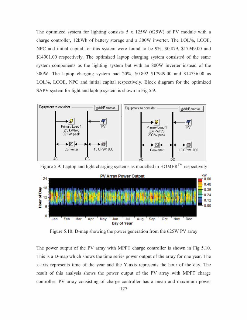
127
The optimized system for lighting consists 5 x 125W (625W) of PV module with a
charge controller, 12kWh of battery storage and a 300W inverter. The LOL%, LCOE,
NPC and initial capital for this system were found to be 9%, $0.879, $17949.00 and
$14001.00 respectively. The optimized laptop charging system consisted of the same
system components as the lighting system but with an 800W inverter instead of the
300W. The laptop charging system had 20%, $0.892 $17949.00 and $14736.00 as
LOL%, LCOE, NPC and initial capital respectively. Block diagram for the optimized
SAPV system for light and laptop system is shown in Fig 5.9.
Figure 5.9: Laptop and light charging systems as modelled in HOMERTM respectively
Figure 5.10: D-map showing the power generation from the 625W PV array
The power output of the PV array with MPPT charge controller is shown in Fig 5.10.
This is a D-map which shows the time series power output of the array for one year. The
x-axis represents time of the year and the Y-axis represents the hour of the day. The
result of this analysis shows the power output of the PV array with MPPT charge
controller. PV array consisting of charge controller has a mean and maximum power
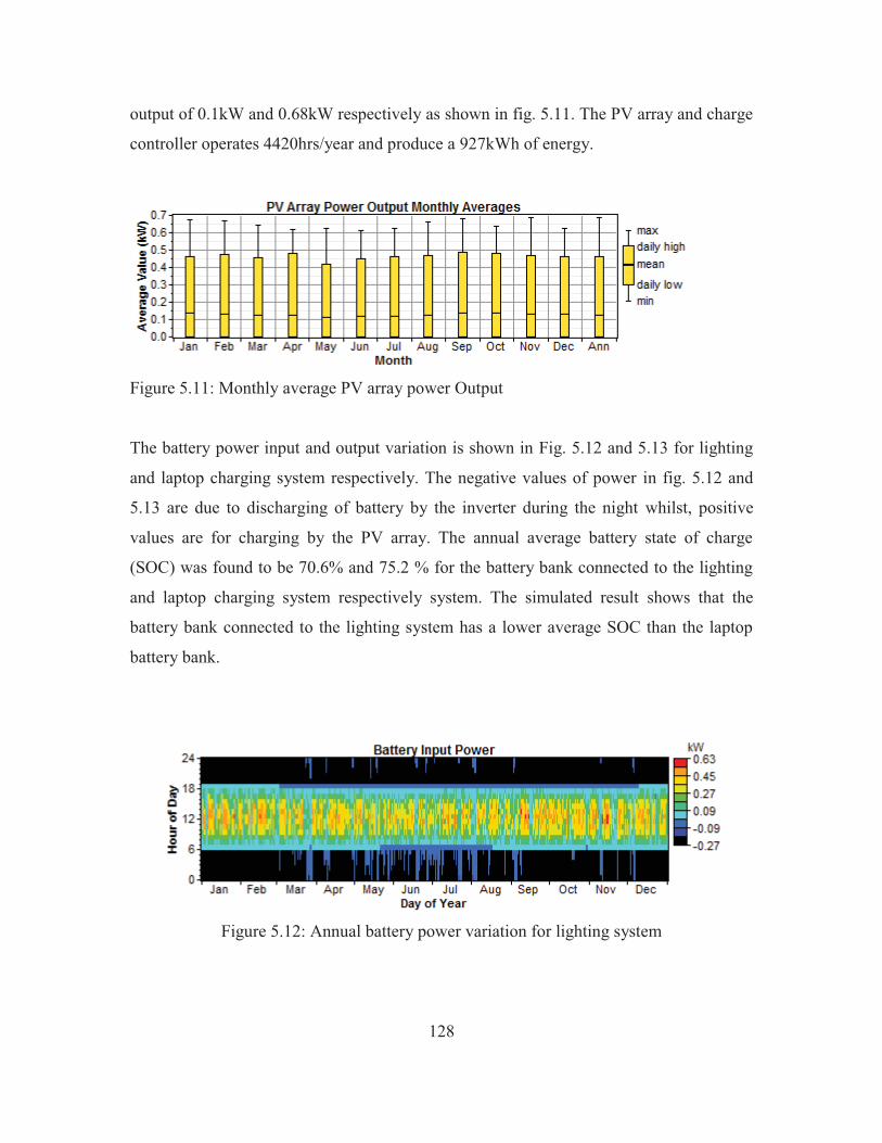
128
output of 0.1kW and 0.68kW respectively as shown in fig. 5.11. The PV array and charge
controller operates 4420hrs/year and produce a 927kWh of energy.
Figure 5.11: Monthly average PV array power Output
The battery power input and output variation is shown in Fig. 5.12 and 5.13 for lighting
and laptop charging system respectively. The negative values of power in fig. 5.12 and
5.13 are due to discharging of battery by the inverter during the night whilst, positive
values are for charging by the PV array. The annual average battery state of charge
(SOC) was found to be 70.6% and 75.2 % for the battery bank connected to the lighting
and laptop charging system respectively system. The simulated result shows that the
battery bank connected to the lighting system has a lower average SOC than the laptop
battery bank.
Figure 5.12: Annual battery power variation for lighting system
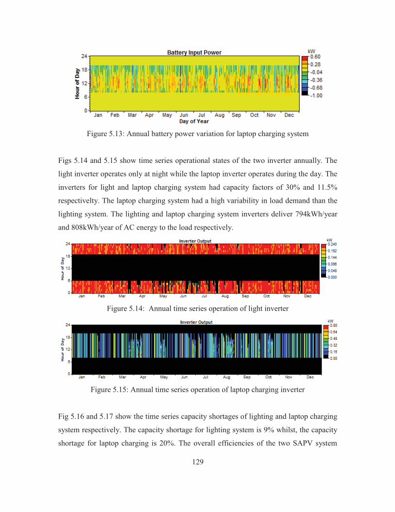
129
Figure 5.13: Annual battery power variation for laptop charging system
Figs 5.14 and 5.15 show time series operational states of the two inverter annually. The
light inverter operates only at night while the laptop inverter operates during the day. The
inverters for light and laptop charging system had capacity factors of 30% and 11.5%
respectivelty. The laptop charging system had a high variability in load demand than the
lighting system. The lighting and laptop charging system inverters deliver 794kWh/year
and 808kWh/year of AC energy to the load respectively.
Figure 5.14: Annual time series operation of light inverter
Figure 5.15: Annual time series operation of laptop charging inverter
Fig 5.16 and 5.17 show the time series capacity shortages of lighting and laptop charging
system respectively. The capacity shortage for lighting system is 9% whilst, the capacity
shortage for laptop charging is 20%. The overall efficiencies of the two SAPV system
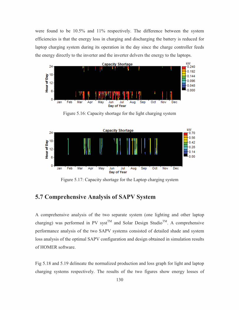
130
were found to be 10.5% and 11% respectively. The difference between the system
efficiencies is that the energy loss in charging and discharging the battery is reduced for
laptop charging system during its operation in the day since the charge controller feeds
the energy directly to the inverter and the inverter delvers the energy to the laptops.
Figure 5.16: Capacity shortage for the light charging system
Figure 5.17: Capacity shortage for the Laptop charging system
5.7 Comprehensive Analysis of SAPV System
A comprehensive analysis of the two separate system (one lighting and other laptop
charging) was performed in PV systTM and Solar Design StudioTM. A comprehensive
performance analysis of the two SAPV systems consisted of detailed shade and system
loss analysis of the optimal SAPV configuration and design obtained in simulation results
of HOMER software.
Fig 5.18 and 5.19 delineate the normalized production and loss graph for light and laptop
charging systems respectively. The results of the two figures show energy losses of
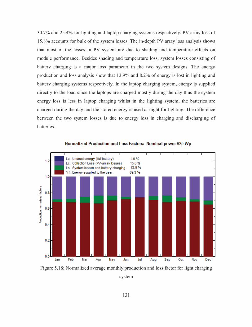
131
30.7% and 25.4% for lighting and laptop charging systems respectively. PV array loss of
15.8% accounts for bulk of the system losses. The in-depth PV array loss analysis shows
that most of the losses in PV system are due to shading and temperature effects on
module performance. Besides shading and temperature loss, system losses consisting of
battery charging is a major loss parameter in the two system designs. The energy
production and loss analysis show that 13.9% and 8.2% of energy is lost in lighting and
battery charging systems respectively. In the laptop charging system, energy is supplied
directly to the load since the laptops are charged mostly during the day thus the system
energy loss is less in laptop charging whilst in the lighting system, the batteries are
charged during the day and the stored energy is used at night for lighting. The difference
between the two system losses is due to energy loss in charging and discharging of
batteries.
Figure 5.18: Normalized average monthly production and loss factor for light charging
system
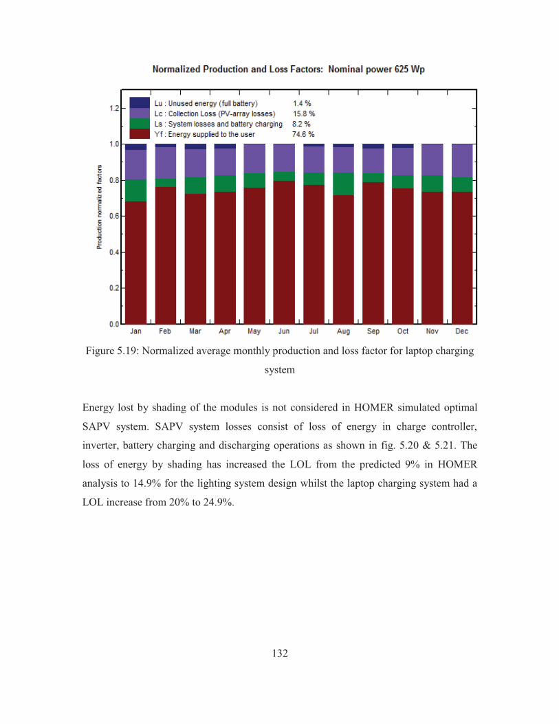
132
Figure 5.19: Normalized average monthly production and loss factor for laptop charging
system
Energy lost by shading of the modules is not considered in HOMER simulated optimal
SAPV system. SAPV system losses consist of loss of energy in charge controller,
inverter, battery charging and discharging operations as shown in fig. 5.20 & 5.21. The
loss of energy by shading has increased the LOL from the predicted 9% in HOMER
analysis to 14.9% for the lighting system design whilst the laptop charging system had a
LOL increase from 20% to 24.9%.
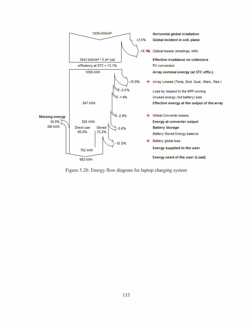
133
Figure 5.20: Energy flow diagram for laptop charging system
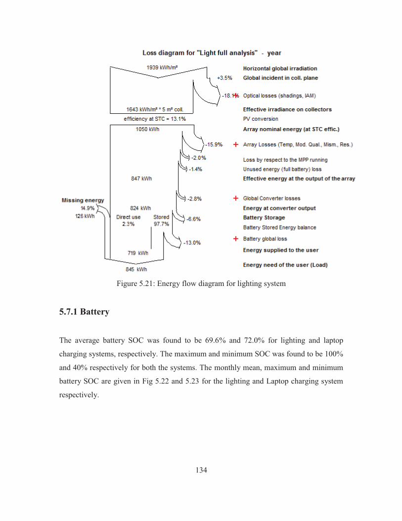
134
Figure 5.21: Energy flow diagram for lighting system
5.7.1 Battery
The average battery SOC was found to be 69.6% and 72.0% for lighting and laptop
charging systems, respectively. The maximum and minimum SOC was found to be 100%
and 40% respectively for both the systems. The monthly mean, maximum and minimum
battery SOC are given in Fig 5.22 and 5.23 for the lighting and Laptop charging system
respectively.
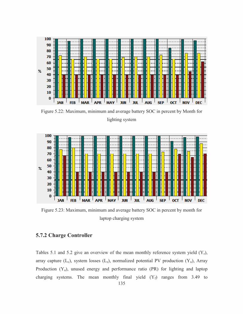
135
Figure 5.22: Maximum, minimum and average battery SOC in percent by Month for
lighting system
Figure 5.23: Maximum, minimum and average battery SOC in percent by month for
laptop charging system
5.7.2 Charge Controller
Tables 5.1 and 5.2 give an overview of the mean monthly reference system yield (Yr),
array capture (Lc), system losses (Ls), normalized potential PV production (Yu), Array
Production (Ya), unused energy and performance ratio (PR) for lighting and laptop
charging systems. The mean monthly final yield (Yf) ranges from 3.49 to
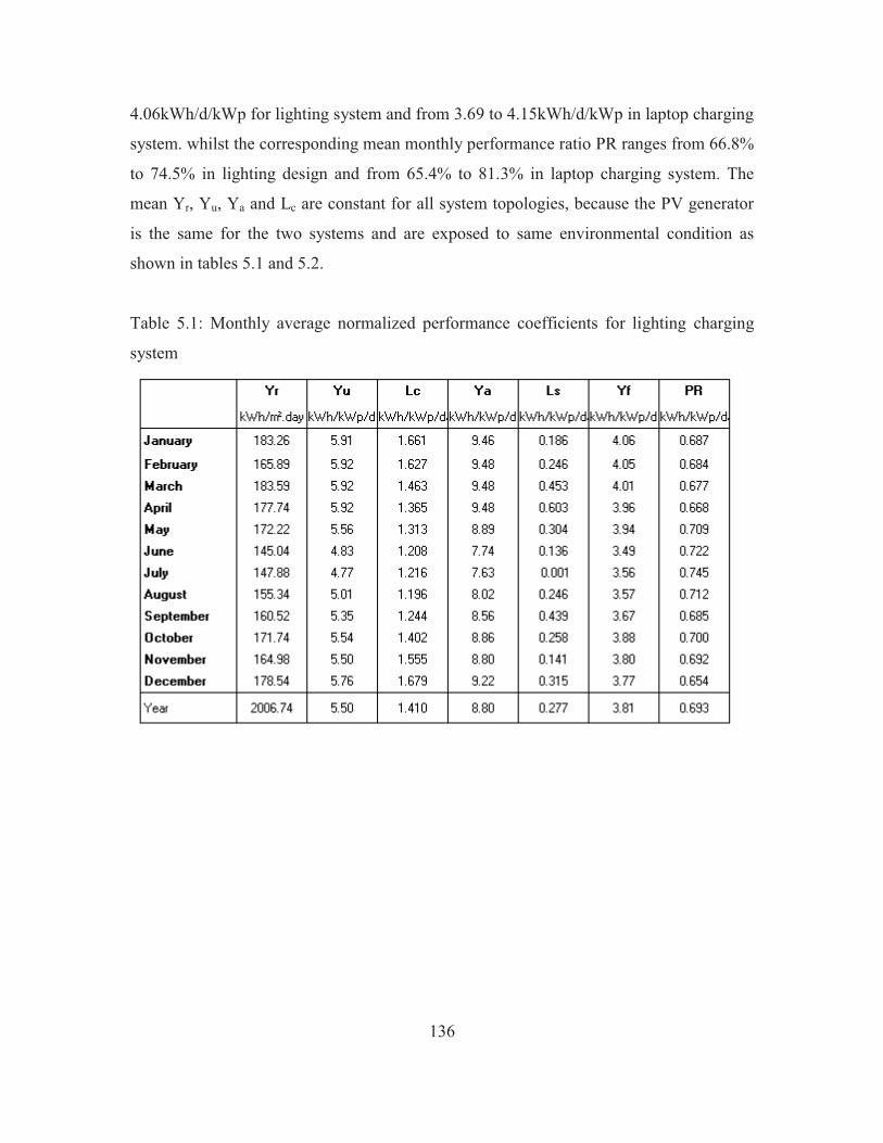
136
4.06kWh/d/kWp for lighting system and from 3.69 to 4.15kWh/d/kWp in laptop charging
system. whilst the corresponding mean monthly performance ratio PR ranges from 66.8%
to 74.5% in lighting design and from 65.4% to 81.3% in laptop charging system. The
mean Yr, Yu, Ya and Lc are constant for all system topologies, because the PV generator
is the same for the two systems and are exposed to same environmental condition as
shown in tables 5.1 and 5.2.
Table 5.1: Monthly average normalized performance coefficients for lighting charging
system
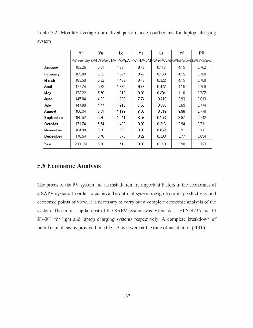
137
Table 5.2: Monthly average normalized performance coefficients for laptop charging
system
5.8 Economic Analysis
The prices of the PV system and its installation are important factors in the economics of
a SAPV system. In order to achieve the optimal system design from its productivity and
economic points of view, it is necessary to carry out a complete economic analysis of the
system. The initial capital cost of the SAPV system was estimated at FJ $14736 and FJ
$14001 for light and laptop charging systems respectively. A complete breakdown of
initial capital cost is provided in table 5.3 as it were at the time of installation (2010).
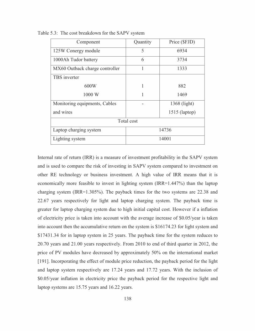
138
Table 5.3: The cost breakdown for the SAPV system
Component Quantity Price ($FJD)
125W Conergy module 5 6934
1000Ah Tudor battery 6 3734
MX60 Outback charge controller 1 1333
TBS inverter
600W
1000 W
1
1
882
1469
Monitoring equipments, Cables
and wires
- 1368 (light)
1515 (laptop)
Total cost
Laptop charging system 14736
Lighting system 14001
Internal rate of return (IRR) is a measure of investment profitability in the SAPV system
and is used to compare the risk of investing in SAPV system compared to investment on
other RE technology or business investment. A high value of IRR means that it is
economically more feasible to invest in lighting system (IRR=1.447%) than the laptop
charging system (IRR=1.305%). The payback times for the two systems are 22.38 and
22.67 years respectively for light and laptop charging system. The payback time is
greater for laptop charging system due to high initial capital cost. However if a inflation
of electricity price is taken into account with the average increase of $0.05/year is taken
into account then the accumulative return on the system is $16174.23 for light system and
$17431.34 for in laptop system in 25 years. The payback time for the system reduces to
20.70 years and 21.00 years respectively. From 2010 to end of third quarter in 2012, the
price of PV modules have decreased by approximately 50% on the international market
[191]. Incorporating the effect of module price reduction, the payback period for the light
and laptop system respectively are 17.24 years and 17.72 years. With the inclusion of
$0.05/year inflation in electricity price the payback period for the respective light and
laptop systems are 15.75 years and 16.22 years.
139
The payback periods for the respective systems will be far less than what has been
calculated above if the current SAPV system is compared with remote power
technologies such as diesel generators in outer islands were the price of diesel is higher
than price on mainland.
5.9 Sensitivity Analysis
An eight dimension sensitivity analysis was carried out in HOMER software to
understand the viability of standalone system in power generation under different
operating and environmental conditions. The sensitivity analysis was performed on
LCOE, total capital cost and NPC as shown in figs 5.24-5.26. The results of sensitivity
analysis show that economic feasibility and viability of SAPV system are dependent on
system component cost and environmental parameters that drive the energy generation.
The eight dimension sensitivity parameters consisted of PV module, battery and battery
replacement cost, global radiation, project lifetime, load, inverter life and capacity
shortage.
The sensitivity analysis of LCOE delineates that the cost of energy is a strong function of
PV module price, battery price and the global radiation at the location. Reduction of PV
module and battery prices by 25% reduces the LCOE to $0.74 kWh. The average
insolation in Fiji varies from 3.7kWhm-2 to 7.1kWhm-2 and, based on this sensitivity
parameter alone, the cost of energy from SAPV can vary from $0.80/kWh to $1.15/kWh.
However, if the insolation variation in Fiji is coupled with 25% reductions in PV module
and battery price the LCOE will vary from $0.58/kWh to $1.10/kWh as shown in Fig
5.24.
The sensitivity analysis of capital cost and NPC shows that the cost of installation of a
new system is heavily dependent on the load and the local solar insolation. An increase in
solar radiation (a different location) decreases the initial capital to the system whilst an
increase in load obviously increases the initial capital needs.
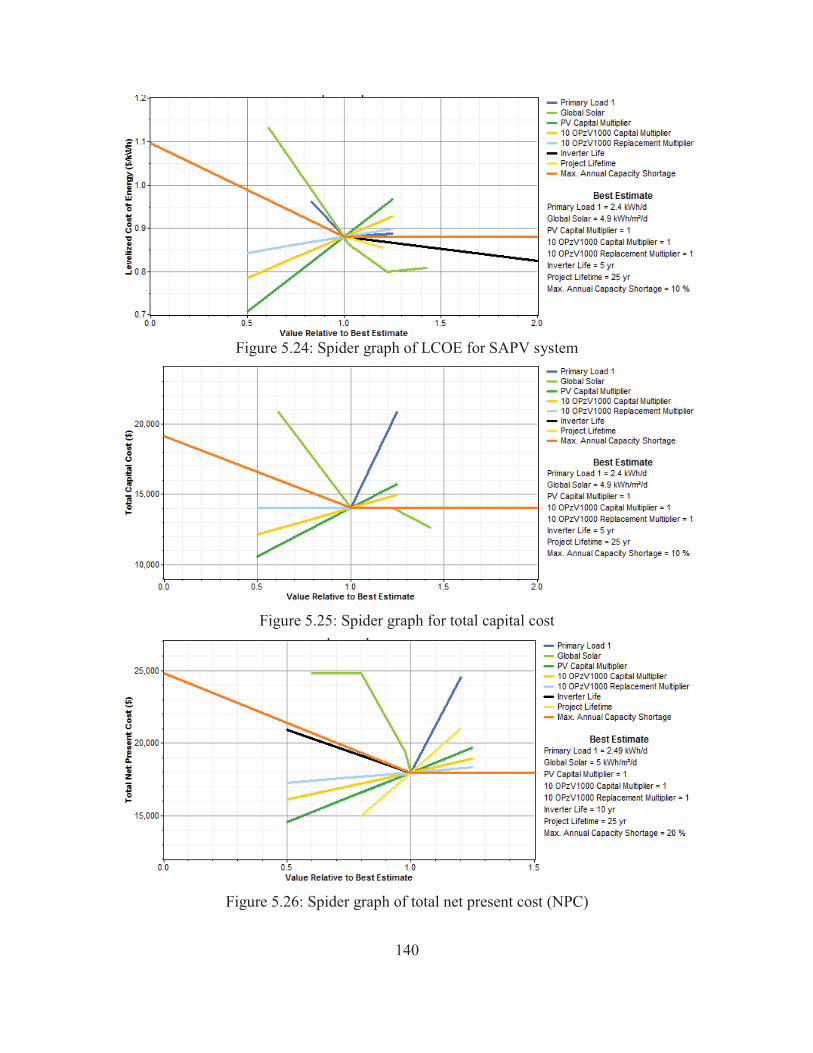
140
Figure 5.24: Spider graph of LCOE for SAPV system
Figure 5.25: Spider graph for total capital cost
Figure 5.26: Spider graph of total net present cost (NPC)
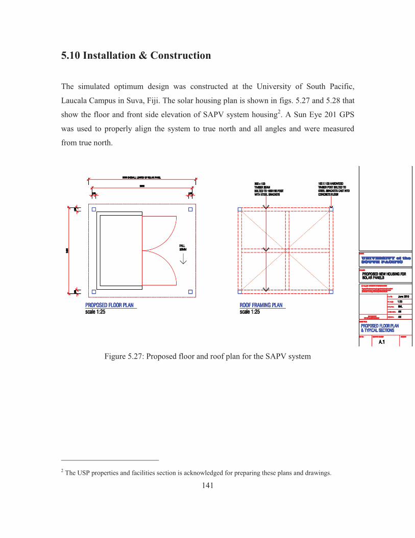
141
5.10 Installation & Construction
The simulated optimum design was constructed at the University of South Pacific,
Laucala Campus in Suva, Fiji. The solar housing plan is shown in figs. 5.27 and 5.28 that
show the floor and front side elevation of SAPV system housing2. A Sun Eye 201 GPS
was used to properly align the system to true north and all angles and were measured
from true north.
Figure 5.27: Proposed floor and roof plan for the SAPV system
2 The USP properties and facilities section is acknowledged for preparing these plans and drawings.
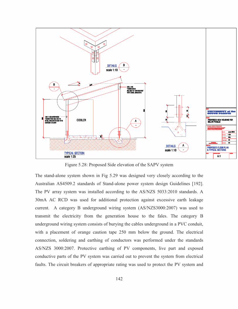
142
Figure 5.28: Proposed Side elevation of the SAPV system
The stand-alone system shown in Fig 5.29 was designed very closely according to the
Australian AS4509.2 standards of Stand-alone power system design Guidelines [192].
The PV array system was installed according to the AS/NZS 5033:2010 standards. A
30mA AC RCD was used for additional protection against excessive earth leakage
current. A category B underground wiring system (AS/NZS3000:2007) was used to
transmit the electricity from the generation house to the fales. The category B
underground wiring system consists of burying the cables underground in a PVC conduit,
with a placement of orange caution tape 250 mm below the ground. The electrical
connection, soldering and earthing of conductors was performed under the standards
AS/NZS 3000:2007. Protective earthing of PV components, live part and exposed
conductive parts of the PV system was carried out to prevent the system from electrical
faults. The circuit breakers of appropriate rating was used to protect the PV system and
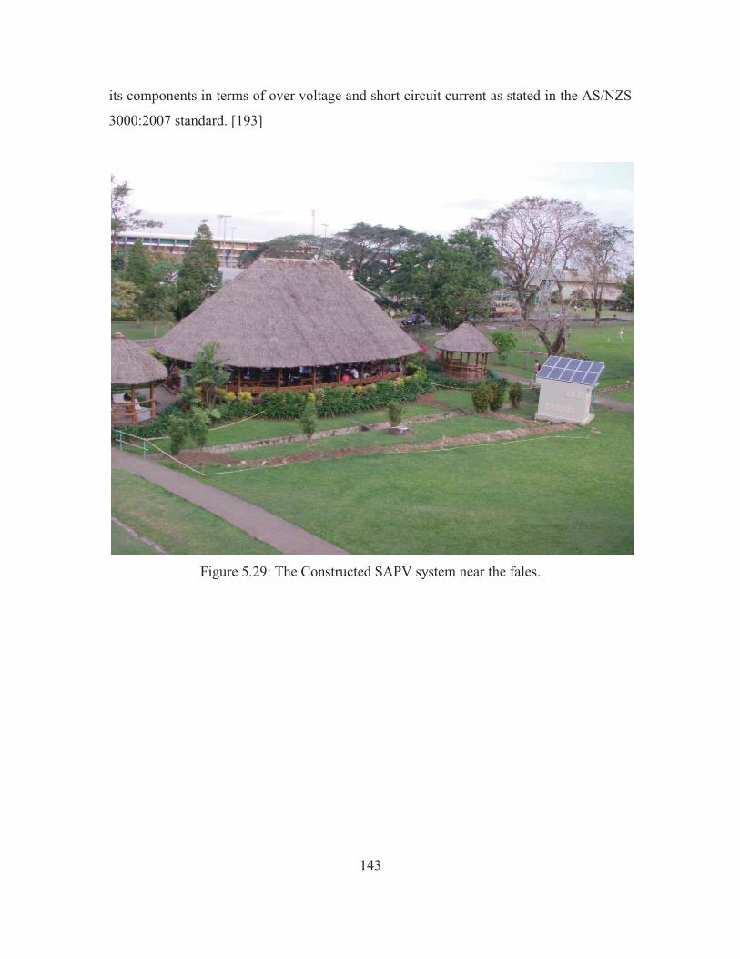
143
its components in terms of over voltage and short circuit current as stated in the AS/NZS
3000:2007 standard. [193]
Figure 5.29: The Constructed SAPV system near the fales.
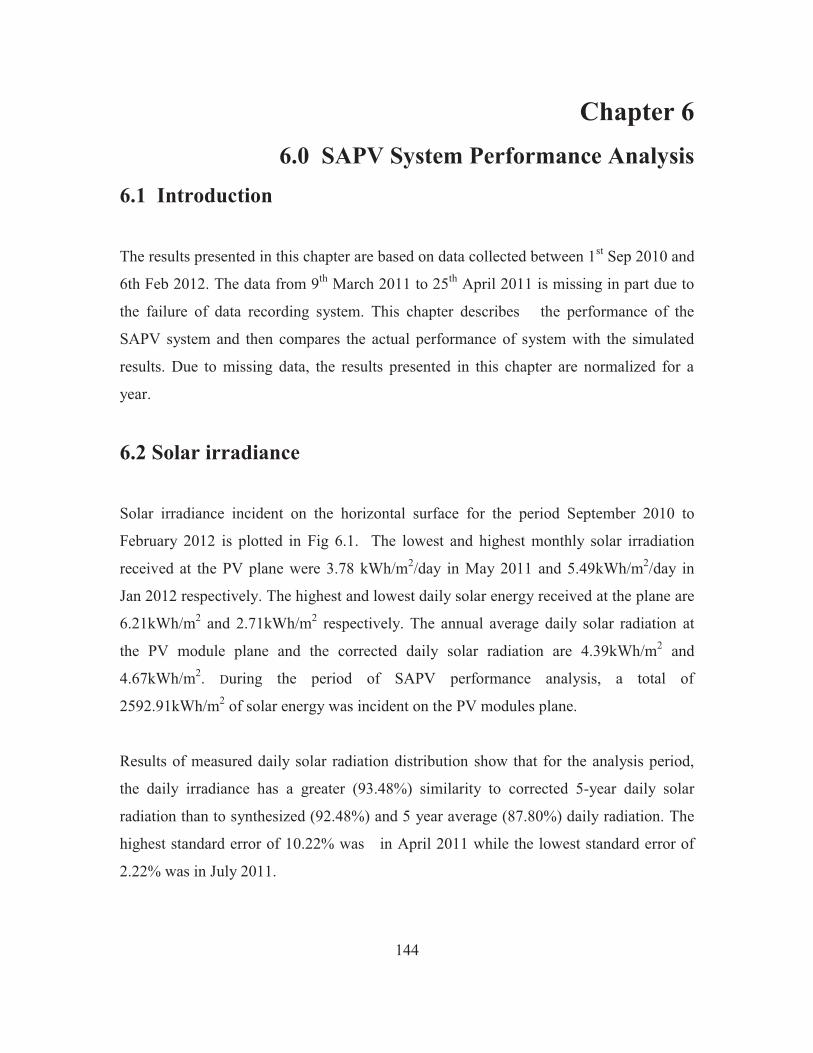
144
Chapter 6 6.0 SAPV System Performance Analysis
6.1 Introduction
The results presented in this chapter are based on data collected between 1st Sep 2010 and
6th Feb 2012. The data from 9th March 2011 to 25th April 2011 is missing in part due to
the failure of data recording system. This chapter describes the performance of the
SAPV system and then compares the actual performance of system with the simulated
results. Due to missing data, the results presented in this chapter are normalized for a
year.
6.2 Solar irradiance
Solar irradiance incident on the horizontal surface for the period September 2010 to
February 2012 is plotted in Fig 6.1. The lowest and highest monthly solar irradiation
received at the PV plane were 3.78 kWh/m2/day in May 2011 and 5.49kWh/m2/day in
Jan 2012 respectively. The highest and lowest daily solar energy received at the plane are
6.21kWh/m2 and 2.71kWh/m2 respectively. The annual average daily solar radiation at
the PV module plane and the corrected daily solar radiation are 4.39kWh/m2 and
4.67kWh/m2. During the period of SAPV performance analysis, a total of
2592.91kWh/m2 of solar energy was incident on the PV modules plane.
Results of measured daily solar radiation distribution show that for the analysis period,
the daily irradiance has a greater (93.48%) similarity to corrected 5-year daily solar
radiation than to synthesized (92.48%) and 5 year average (87.80%) daily radiation. The
highest standard error of 10.22% was in April 2011 while the lowest standard error of
2.22% was in July 2011.
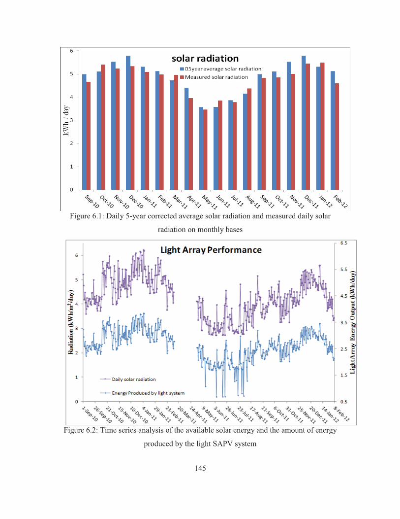
145
Figure 6.1: Daily 5-year corrected average solar radiation and measured daily solar
radiation on monthly bases
Figure 6.2: Time series analysis of the available solar energy and the amount of energy
produced by the light SAPV system
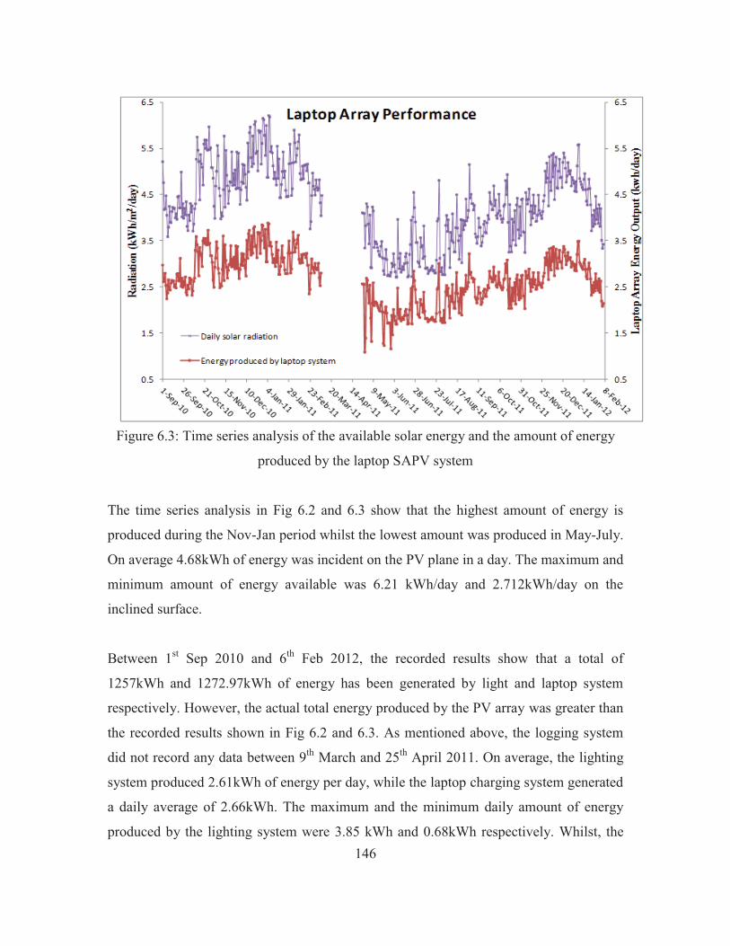
146
Figure 6.3: Time series analysis of the available solar energy and the amount of energy
produced by the laptop SAPV system
The time series analysis in Fig 6.2 and 6.3 show that the highest amount of energy is
produced during the Nov-Jan period whilst the lowest amount was produced in May-July.
On average 4.68kWh of energy was incident on the PV plane in a day. The maximum and
minimum amount of energy available was 6.21 kWh/day and 2.712kWh/day on the
inclined surface.
Between 1st Sep 2010 and 6th Feb 2012, the recorded results show that a total of
1257kWh and 1272.97kWh of energy has been generated by light and laptop system
respectively. However, the actual total energy produced by the PV array was greater than
the recorded results shown in Fig 6.2 and 6.3. As mentioned above, the logging system
did not record any data between 9th March and 25th April 2011. On average, the lighting
system produced 2.61kWh of energy per day, while the laptop charging system generated
a daily average of 2.66kWh. The maximum and the minimum daily amount of energy
produced by the lighting system were 3.85 kWh and 0.68kWh respectively. Whilst, the
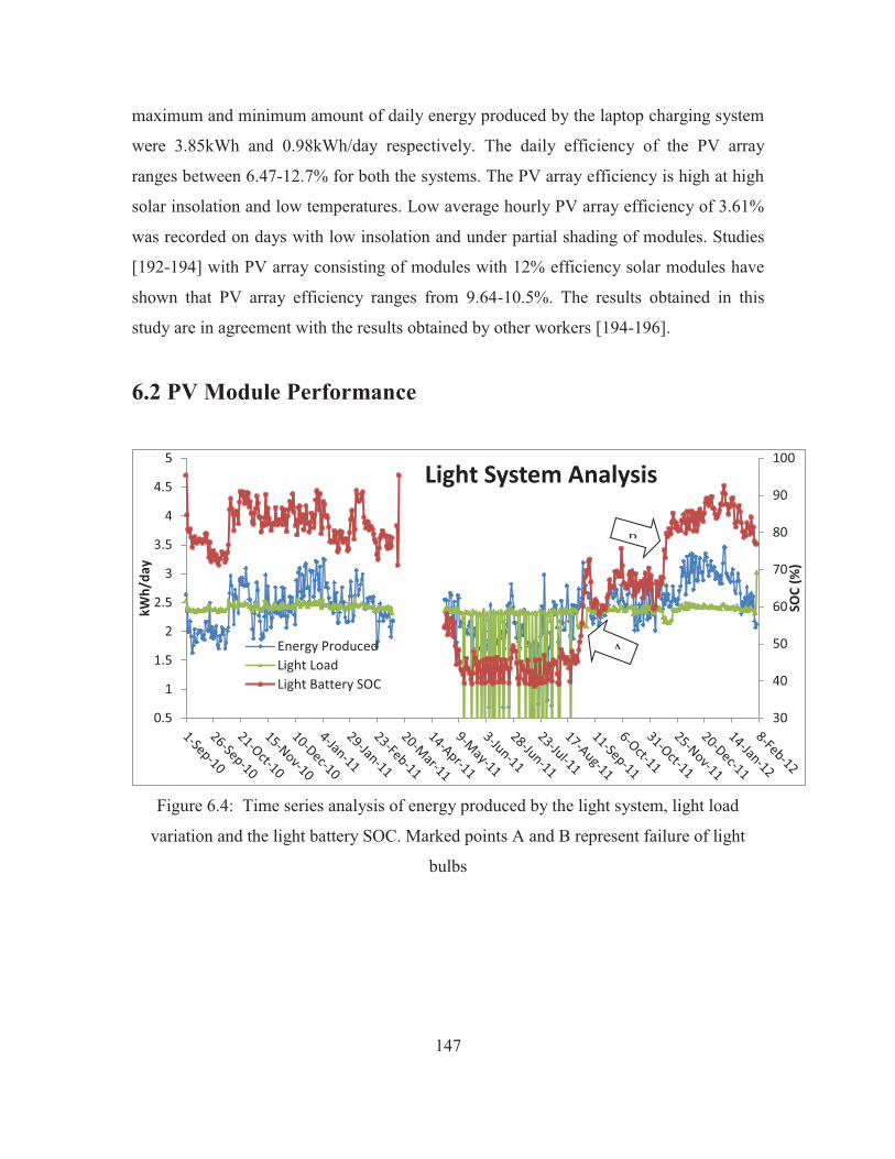
147
maximum and minimum amount of daily energy produced by the laptop charging system
were 3.85kWh and 0.98kWh/day respectively. The daily efficiency of the PV array
ranges between 6.47-12.7% for both the systems. The PV array efficiency is high at high
solar insolation and low temperatures. Low average hourly PV array efficiency of 3.61%
was recorded on days with low insolation and under partial shading of modules. Studies
[192-194] with PV array consisting of modules with 12% efficiency solar modules have
shown that PV array efficiency ranges from 9.64-10.5%. The results obtained in this
study are in agreement with the results obtained by other workers [194-196].
6.2 PV Module Performance
Figure 6.4: Time series analysis of energy produced by the light system, light load
variation and the light battery SOC. Marked points A and B represent failure of light
bulbs
30
40
50
60
70
80
90
100
0.5
1
1.5
2
2.5
3
3.5
4
4.5
5
SOC
(%)
kWh/
day
Light System Analysis
Energy ProducedLight LoadLight Battery SOC
A
B
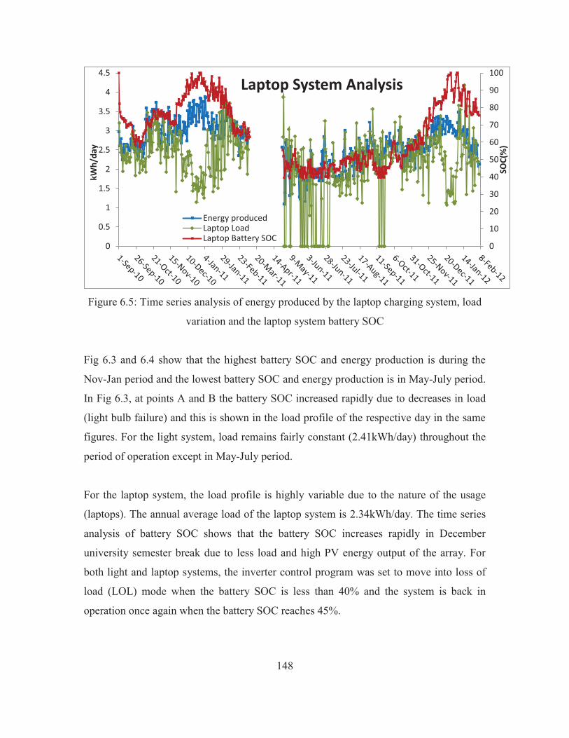
148
Figure 6.5: Time series analysis of energy produced by the laptop charging system, load
variation and the laptop system battery SOC
Fig 6.3 and 6.4 show that the highest battery SOC and energy production is during the
Nov-Jan period and the lowest battery SOC and energy production is in May-July period.
In Fig 6.3, at points A and B the battery SOC increased rapidly due to decreases in load
(light bulb failure) and this is shown in the load profile of the respective day in the same
figures. For the light system, load remains fairly constant (2.41kWh/day) throughout the
period of operation except in May-July period.
For the laptop system, the load profile is highly variable due to the nature of the usage
(laptops). The annual average load of the laptop system is 2.34kWh/day. The time series
analysis of battery SOC shows that the battery SOC increases rapidly in December
university semester break due to less load and high PV energy output of the array. For
both light and laptop systems, the inverter control program was set to move into loss of
load (LOL) mode when the battery SOC is less than 40% and the system is back in
operation once again when the battery SOC reaches 45%.
0
10
20
30
40
50
60
70
80
90
100
0
0.5
1
1.5
2
2.5
3
3.5
4
4.5
SOC(
%)
kWh/
day
Laptop System Analysis
Energy producedLaptop LoadLaptop Battery SOC
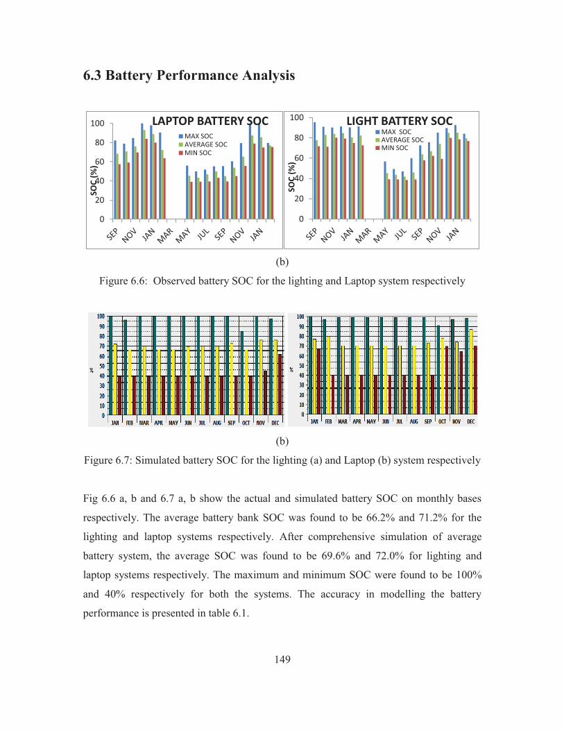
149
6.3 Battery Performance Analysis
(b)
Figure 6.6: Observed battery SOC for the lighting and Laptop system respectively
(b)
Figure 6.7: Simulated battery SOC for the lighting (a) and Laptop (b) system respectively
Fig 6.6 a, b and 6.7 a, b show the actual and simulated battery SOC on monthly bases
respectively. The average battery bank SOC was found to be 66.2% and 71.2% for the
lighting and laptop systems respectively. After comprehensive simulation of average
battery system, the average SOC was found to be 69.6% and 72.0% for lighting and
laptop systems respectively. The maximum and minimum SOC were found to be 100%
and 40% respectively for both the systems. The accuracy in modelling the battery
performance is presented in table 6.1.
0
20
40
60
80
100
SOC
(%)
LAPTOP BATTERY SOC MAX SOCAVERAGE SOCMIN SOC
0
20
40
60
80
100
SOC
(%)
LIGHT BATTERY SOC MAX SOCAVERAGE SOCMIN SOC
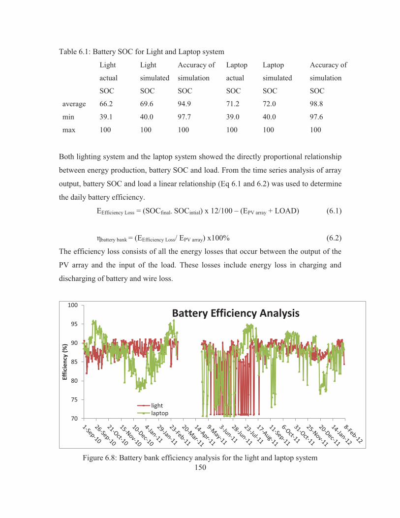
150
Table 6.1: Battery SOC for Light and Laptop system
Light
actual
SOC
Light
simulated
SOC
Accuracy of
simulation
SOC
Laptop
actual
SOC
Laptop
simulated
SOC
Accuracy of
simulation
SOC
average 66.2 69.6 94.9 71.2 72.0 98.8
min 39.1 40.0 97.7 39.0 40.0 97.6
max 100 100 100 100 100 100
Both lighting system and the laptop system showed the directly proportional relationship
between energy production, battery SOC and load. From the time series analysis of array
output, battery SOC and load a linear relationship (Eq 6.1 and 6.2) was used to determine
the daily battery efficiency.
EEfficiency Loss = (SOCfinal- SOCintial) x 12/100 – (EPV array + LOAD) (6.1)
ηbattery bank = (EEfficiency Loss/ EPV array) x100% (6.2)
The efficiency loss consists of all the energy losses that occur between the output of the
PV array and the input of the load. These losses include energy loss in charging and
discharging of battery and wire loss.
Figure 6.8: Battery bank efficiency analysis for the light and laptop system
70
75
80
85
90
95
100
Effic
ienc
y (%
)
Battery Efficiency Analysis
lightlaptop
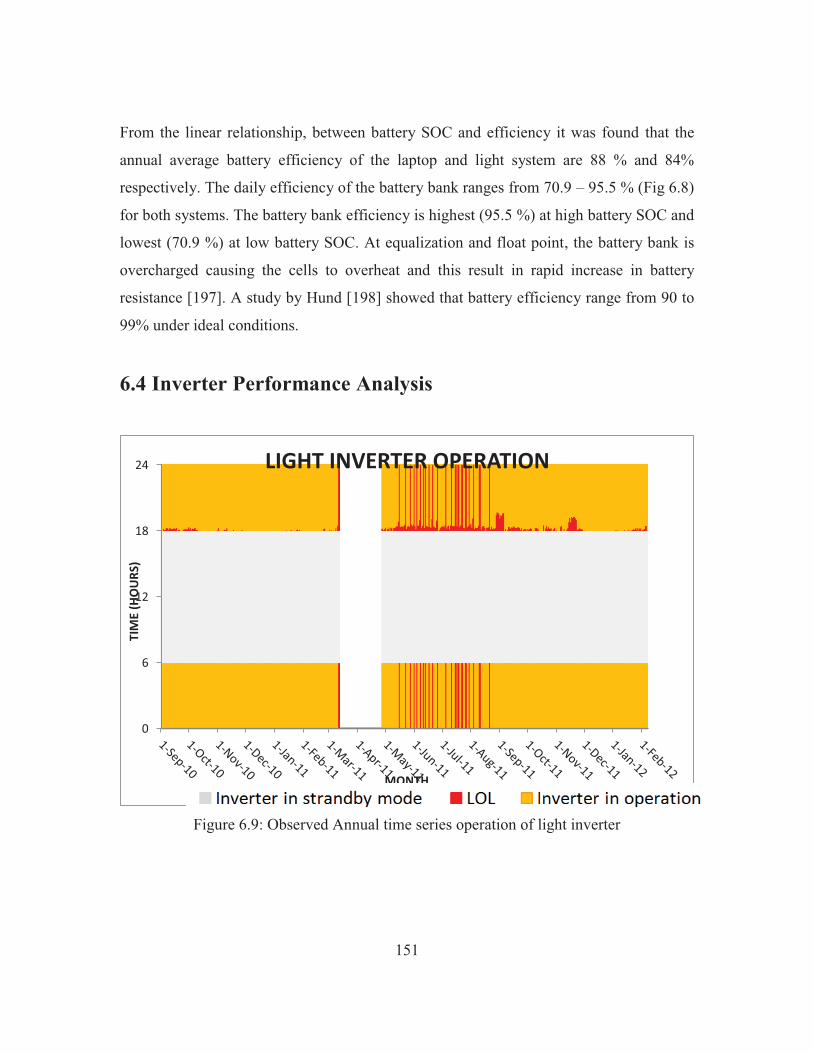
151
From the linear relationship, between battery SOC and efficiency it was found that the
annual average battery efficiency of the laptop and light system are 88 % and 84%
respectively. The daily efficiency of the battery bank ranges from 70.9 – 95.5 % (Fig 6.8)
for both systems. The battery bank efficiency is highest (95.5 %) at high battery SOC and
lowest (70.9 %) at low battery SOC. At equalization and float point, the battery bank is
overcharged causing the cells to overheat and this result in rapid increase in battery
resistance [197]. A study by Hund [198] showed that battery efficiency range from 90 to
99% under ideal conditions.
6.4 Inverter Performance Analysis
Figure 6.9: Observed Annual time series operation of light inverter
0
6
12
18
24
TIM
E (H
OU
RS)
MONTH
LIGHT INVERTER OPERATION
MORNING LOL DAY LOL EVENING
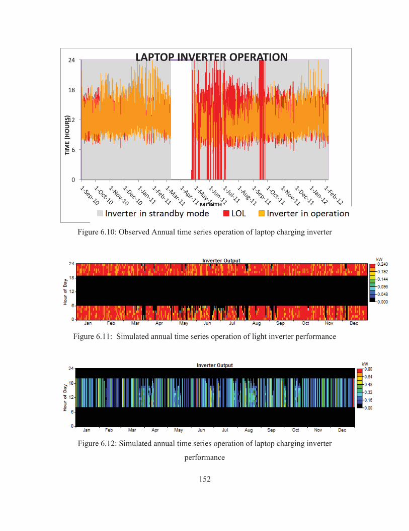
152
Figure 6.10: Observed Annual time series operation of laptop charging inverter
Figure 6.11: Simulated annual time series operation of light inverter performance
Figure 6.12: Simulated annual time series operation of laptop charging inverter
performance
0
6
12
18
24TI
ME
(HO
URS
)
MONTH
LAPTOP INVERTER OPERATION
Inverter in strandby mode LOL LOL Inverter in operation LOL start time
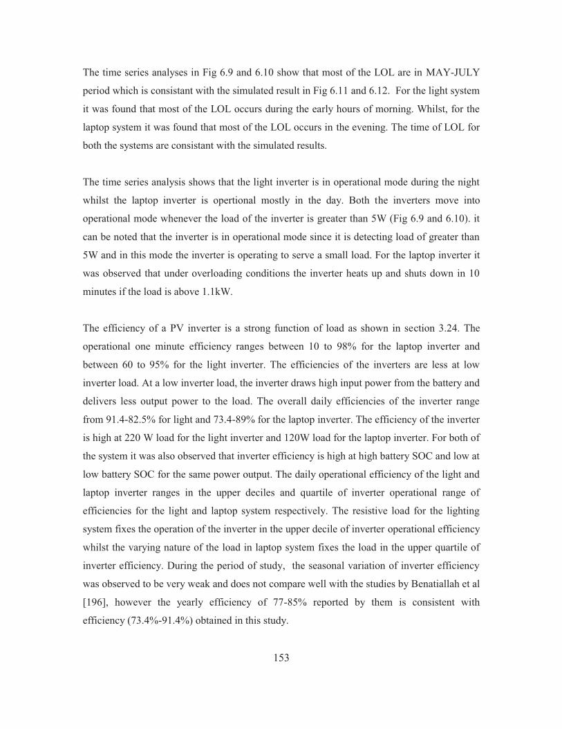
153
The time series analyses in Fig 6.9 and 6.10 show that most of the LOL are in MAY-JULY
period which is consistant with the simulated result in Fig 6.11 and 6.12. For the light system
it was found that most of the LOL occurs during the early hours of morning. Whilst, for the
laptop system it was found that most of the LOL occurs in the evening. The time of LOL for
both the systems are consistant with the simulated results.
The time series analysis shows that the light inverter is in operational mode during the night
whilst the laptop inverter is opertional mostly in the day. Both the inverters move into
operational mode whenever the load of the inverter is greater than 5W (Fig 6.9 and 6.10). it
can be noted that the inverter is in operational mode since it is detecting load of greater than
5W and in this mode the inverter is operating to serve a small load. For the laptop inverter it
was observed that under overloading conditions the inverter heats up and shuts down in 10
minutes if the load is above 1.1kW.
The efficiency of a PV inverter is a strong function of load as shown in section 3.24. The
operational one minute efficiency ranges between 10 to 98% for the laptop inverter and
between 60 to 95% for the light inverter. The efficiencies of the inverters are less at low
inverter load. At a low inverter load, the inverter draws high input power from the battery and
delivers less output power to the load. The overall daily efficiencies of the inverter range
from 91.4-82.5% for light and 73.4-89% for the laptop inverter. The efficiency of the inverter
is high at 220 W load for the light inverter and 120W load for the laptop inverter. For both of
the system it was also observed that inverter efficiency is high at high battery SOC and low at
low battery SOC for the same power output. The daily operational efficiency of the light and
laptop inverter ranges in the upper deciles and quartile of inverter operational range of
efficiencies for the light and laptop system respectively. The resistive load for the lighting
system fixes the operation of the inverter in the upper decile of inverter operational efficiency
whilst the varying nature of the load in laptop system fixes the load in the upper quartile of
inverter efficiency. During the period of study, the seasonal variation of inverter efficiency
was observed to be very weak and does not compare well with the studies by Benatiallah et al
[196], however the yearly efficiency of 77-85% reported by them is consistent with
efficiency (73.4%-91.4%) obtained in this study.
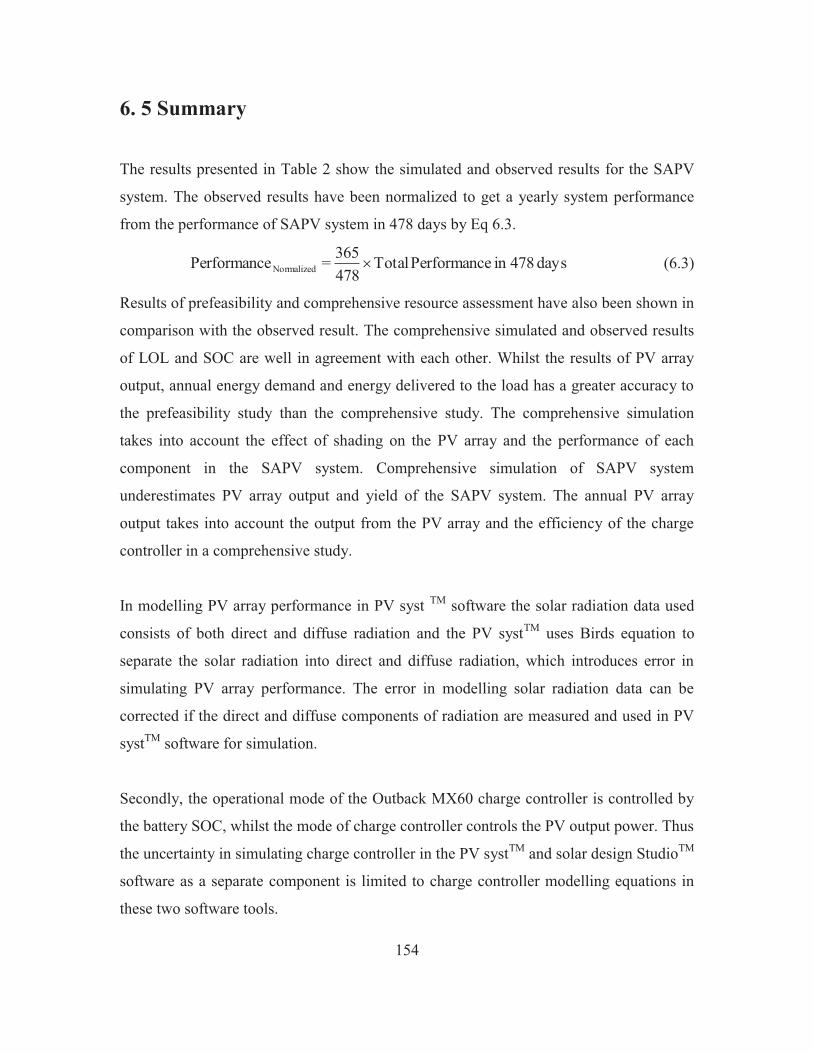
154
6. 5 Summary
The results presented in Table 2 show the simulated and observed results for the SAPV
system. The observed results have been normalized to get a yearly system performance
from the performance of SAPV system in 478 days by Eq 6.3.
days 478in ePerformanc Total478365 = ePerformanc Normalized � (6.3)
Results of prefeasibility and comprehensive resource assessment have also been shown in
comparison with the observed result. The comprehensive simulated and observed results
of LOL and SOC are well in agreement with each other. Whilst the results of PV array
output, annual energy demand and energy delivered to the load has a greater accuracy to
the prefeasibility study than the comprehensive study. The comprehensive simulation
takes into account the effect of shading on the PV array and the performance of each
component in the SAPV system. Comprehensive simulation of SAPV system
underestimates PV array output and yield of the SAPV system. The annual PV array
output takes into account the output from the PV array and the efficiency of the charge
controller in a comprehensive study.
In modelling PV array performance in PV syst TM software the solar radiation data used
consists of both direct and diffuse radiation and the PV systTM uses Birds equation to
separate the solar radiation into direct and diffuse radiation, which introduces error in
simulating PV array performance. The error in modelling solar radiation data can be
corrected if the direct and diffuse components of radiation are measured and used in PV
systTM software for simulation.
Secondly, the operational mode of the Outback MX60 charge controller is controlled by
the battery SOC, whilst the mode of charge controller controls the PV output power. Thus
the uncertainty in simulating charge controller in the PV systTM and solar design StudioTM
software as a separate component is limited to charge controller modelling equations in
these two software tools.
155
The accuracy of simulation ranges between 88-98% and 87-98% for each of the
parameters in Table 2 with respect to the observed results. The highest uncertainty was
observed in determining the LOL in the prefeasibility study. The prefeasibility study
underestimates LOL due HOMERTM software’s inability to model the effect of shading
on PV array performance. The accuracy of comprehensive study in determining LOL and
the overall system performance has increased due to accuracy in simulating PV system
performance with separate system components in PV systTM and Solar Design StudioTM
software.
The results of component testing in chapter 3 has played an instrumental role in
simulating the components of SAPV system and the result has been reflected in high
simulation accuracies with the actual component efficiencies. The overall system
efficiency of SAPV system have been observed to range between 7.22-10.2% by
Benatiallah et al [196] and in this study the overall daily SAPV system efficiency ranges
from 8.8% to 9.1% for both the light and laptop system.
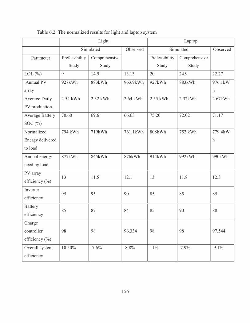
156
Table 6.2: The normalized results for light and laptop system
Light Laptop
Simulated Observed Simulated Observed
Parameter Prefeasibility
Study
Comprehensive
Study
Prefeasibility
Study
Comprehensive
Study
LOL (%) 9 14.9 13.13 20 24.9 22.27
Annual PV
array
927kWh 883kWh 963.9kWh 927kWh 883kWh 976.1kW
h
Average Daily
PV production.
2.54 kWh 2.32 kWh 2.64 kWh 2.55 kWh 2.32kWh 2.67kWh
Average Battery
SOC (%)
70.60 69.6 66.63 75.20 72.02 71.17
Normalized
Energy delivered
to load
794 kWh 719kWh 761.1kWh 808kWh 752 kWh 779.4kW
h
Annual energy
need by load
877kWh 845kWh 876kWh 914kWh 992kWh 990kWh
PV array
efficiency (%) 13 11.5 12.1 13 11.8 12.3
Inverter
efficiency 95 95 90 85 85 85
Battery
efficiency 85 87 84 85 90 88
Charge
controller
efficiency (%)
98 98 96.334 98 98 97.544
Overall system
efficiency
10.50% 7.6% 8.8% 11% 7.9% 9.1%
157
6.6 Conclusion
From the SAPV performance analysis, it can be concluded that individual component
modelling increases simulation accuracies in PV systTM and Solar Design StudioTM
software. The overall efficiency of SAPV system has a higher accuracy to comprehensive
analysis in comparison to prefeasibility study.
The operation efficiency of the light SAPV system is high at high battery SOC and 220W
load and low at low battery SOC. The efficiency is also low at high array temperatures
and partial shading by the nearby trees and building. For the laptop SAPV system the
operational efficiency was found to be high at high battery SOC and under conditions
when the PV array output and the load demand are same. In this case, the battery is not
charged and the PV array output is used directly to serve the load. The efficiency of the
laptop system is low at high array temperatures, low battery SOC and partial shading of
modules. For both the systems it was observed that the overall, SAPV system efficiency
is also low at high solar radiation with full battery SOC and no load demand. In this
situation, the input energy from the sun is high, battery banks are charged to equalization
or float point and the output from the system is low.
158
Chapter 7 7.0 Conclusion and Recommendations
7.1 Solar resource Solar resource assessment is regarded as the basic ingredient necessary for determination
of PV system feasibility. The first part of solar resource assessment consisted of
correcting the recorded solar resource data. The correction of solar resource data
provided a reliable representation of solar resource at the site of the PV system
installation and fulfilled part 2 of AS4509 (2009) standard on use of reliable solar
resource data in designing SAPV system. The solar resource assessment result was used
to determine the site specific optimum tilt and azimuth angle for highest solar access at
the site and maximum annual energy output from the SAPV system. Site specific solar
resource assessment was carried out in order to design a optimum SAPV system to cater
for lighting and laptop charging system at USP. The solar resource assessment consisted
of evaluating the actual solar resource at the site which was affected by shading from
nearby trees and buildings.
The optimal tilt angle for the modules was determined by detailed modelling of buildings
and trees in the vicinity. The optimal azimuth and tilt angles were found to be 15-20° tilt
and 330-350° azimuth from true north. The annual average solar access to direct radiation
on a clear day at the site was found to be 90.3%.
The solar radiation data was corrected for shading effects using Bird’s equations and the
solar access map at the weather station. The corrected and synthesized radiation data
were within 92% in agreement. The annual solar access at the site was found to be 96%
and the annual average corrected solar radiation was calculated to be 4.8 kWhm-2. The
annual corrected horizontal radiation at the Physics division meteorological station is 4.6
kWhm-2 and the calculated solar radiation at the site of installation was found to be 4.8
kWhm-2.
159
7.2 Performance testing and monitoring Performance testing and monitoring consisted of assessment and performance monitoring
of individual components of SAPV and the overall system performance. Chapter 4 details
testing standards and discuss necessary information needed to increases the accuracy of
modelling and analysis of SAPV system by studying the behaviour and response of major
component of SAPV system. The components investigated were solar modules, inverter,
battery and the charge controller.
The IEEE-450 and IEC- 62093 standards were used for battery performance evaluation,
and designing a control algorithm for monitoring of battery performance. The discharging
efficiency from 100 to 40% battery SOC were found to be 91% and 94% for a discharge
load of 850W and 225W respectively. The overall charge-discharge efficiency for cycles
between 40 to 100% battery efficiency was found to be 79% and 81% for 850W and
225W loads respectively. The battery efficiency testing showed that it is highest at 225W
discharge load.
The inverter performance evaluation showed that the efficiency of the inverter was
primarily dependent on load and battery SOC. The efficiencies of the TBS PS 1000-12
and PS 600-12 were found to be highest at 100% battery SOC and 125W and 250W load
for the two inverters respectively. The inverter efficiency was found to have a maximum
of 96.6% under 100% SOC for PS1000-12 inverter at 125W load, whilst PS600-12
inverter had a peak efficiency of 95.1% at 225W load and 100% SOC.
The solar module testing consisted of determination of solar module coefficients at
normal operating conditions for detailed modelling of solar module and to study the
variation of solar module performance under partial shading conditions. The results of
this section were used to set the operational mode of charge controller for optimization of
energy production. The values of solar module coefficients are detailed in table 4.8,
whilst the effect of shading on module performance is shown section 4.542. The results
of shading in table 4.9 and table 4.10 show that the performance of solar module is
160
greatly affected by partial shading and the pattern of shading with respect to cell
interconnection and diode configuration. The decrease in module power due to partial
shading ranges from 88% to 47% with respect to a fully illuminated module. A detailed
monitoring of SAPV system was also done to observe the performance of the PV system
under real time operating conditions. From the analysis of I-V curves under partial
shading conditions, the Upickup mode of MPPT operation was chosen over the park
MPPT mode for optimal performance of SAPV system.
The charge controller testing results showed that the MPPT controller efficiency is
dependent on the mode of charge controller operation. The controller mode of operation
is a function of battery voltage, input power to the controller and the voltage and current
set points. The Outback MX60 charge controller has the highest efficiency of 98% in
bulk and absorb mode of operation. The lowest efficiency was found in float mode. An
average combined charge/discharge efficiency of 85% was observed for a complete
battery cycle variation from 100% - 40% - 100% battery SOC. The average combined
efficiency consisted of the charge controllers operation in float (2hours) and equalise
(1hour) mode.
7.3 Design & Simulation
PV systTM, HOMERTM and Solar design StudioTM software’s were used to design and
simulate two optimum SAPV systems in accordance to AS/NZS 4509 (2009) standard.
The design and simulation results show an optimized SAPV system for lighting
consisting of 625W of PV module with a charge controller, 12kWh of battery storage and
a 300W of inverter. The LOL%, LCOE, NPC and initial capital for this system were
found to be 9%, $0.879, $17949.00 and $14001.00 respectively. The optimized laptop
charging system was similar to the lighting system but with an 800W inverter. The laptop
charging system had a LOL of 20% and $0.892 LCOE. The NPC was $17949.00 and the
initial capital was computed to be $14736.00. The capacity shortage for the lighting
system was 9% whilst the capacity shortage for the laptop charging system was 20%. The
161
overall design efficiencies of the two SAPV system were found to be 10.5% and 11%
respectively. The detailed energy production and loss analysis in section 5.7 showed that
13.9% and 8.2% of generated energy are lost in the lighting and battery charging system
with bulk of the losses confined to storage losses in battery. The loss of energy by partial
shading increased the LOL from the predicted 9% in Homer to 14.9% for the actual
lighting system whilst the laptop charging system had a LOL increase from 20% to
24.9%. The average battery SOC was found to be 69.6% and 72.0% for the lighting and
the laptop charging systems respectively. The maximum and minimum SOC were found
to be 100% and 40% for both the systems. The mean monthly final yield (Yf) for both the
systems ranges from 3.5 to 4.2 kWh/d/kWp with monthly performance ratio (PR) ranging
from 65.4% to 81.3%. Based on IRR, it is economically more feasible to invest in
lighting system (IRR=1.5 %) than the laptop charging system (IRR=1. 3%). The payback
times for the two systems were 22.4 and 22.7 years respectively for light and laptop
charging system. It should be noted that from 2010 to end of third quarter in 2012, the
prices of PV modules have reduced by approximately 50% on the international market
[5]. Incorporating the effect of module price reduction on the payback period for the light
and laptop system reduces to 17.24 and 17.72 years respectively. However, if a
$0.05/year inflation in electricity price is taken into account, the payback period for the
lighting and the laptop charging systems are 15.75 years and 16.22 years. It should be
noted that the electricity prices in Fiji are among the lowest in the region and similar
systems would be economically viable in other PICs where electricity costs are very high.
The average insolation in Fiji varies from 3.7kWhm-2 to 7.1kWhm-2. Based on this
sensitivity parameter alone, the cost of energy from SAPV can vary from $0.80 to $1.15
per kWh. An eight dimension sensitivity analysis was performed on LCOE, total capital
cost and NPC of SAPV system under different operating and environmental conditions.
The results of sensitivity analysis show that economic feasibility and viability of SAPV
system are dependent on system component cost and environmental parameters that drive
the energy generation. The sensitivity analysis of LCOE delineates that the cost of energy
is a strong function of PV module and global radiation. Reduction in PV module and
battery price by 25% reduces the LCOE to $0.74 per kWh. However, if the insolation
162
variation in Fiji is coupled with 25% reductions in PV module and battery price the
LCOE varies between $0.58 and $1.10 per kWh. Furthermore, the analysis of capital cost
and NPC shows that the cost of installation of a new system is heavily dependent on the
load and solar insolation at the location.
7.4 SAPV System Performance Analysis
On average, 4.68kWhm-2/day of energy was incident on the PV module plane (9.9 m2
area) and produced 2.61kWh of energy per day. The daily efficiency of the PV system
ranges from 6.47-12.7% for both the systems. The average battery bank SOC was found
to be 66.3% and 71.2% for the lighting and the laptop charging systems. A
comprehensive simulation of PV system performance shows that average battery SOC
are 69.6% and 72.0% for the lighting and the laptop charging systems respectively. The
average battery efficiency of the laptop and light systems are 88% and 84% respectively.
The overall daily efficiencies of the inverters range from 91.4-82.5% for the light system
and 73.4-89% for the laptop charging system inverter. The charge controller had a peak
efficiency of 98%, however the efficiency was dependent on the mode of charge
controller operation. The actual performance analysis of SAPV system shows that the
normalized annual energy delivered to the load from lighting and laptop charging systems
are 761.1 kWh/year and 779.4 kWh/year respectively.
The SAPV system performance simulation and analysis in table 6.2 showed that the
comprehensive simulation has a high overall accuracy when compared with the actual
performance of SAPV system in contrast to the prefeasibility analysis. With the current
performance of the system, the LCOE are $0.96/kWh and $1.05/kWh for the lighting and
the laptop charging SAPV systems. Furthermore, if the current system is compared with
electricity generation for Island application where transportation of fossil fuel adds to the
bulk of cost ($1.02/kWh) in electricity generation, the IRR increases to 6.6% and 6.5%
for the lighting and laptop charging system respectively. The payback time for the two
systems also reduces to 14.4 and 14.3 years respectively for the lighting and the laptop
163
charging system. This analysis clearly shows that SAPV system is more economical for
small island electricity generation in Fiji where fuel costs are much higher than those on
the major islands. The fuel cost on smaller islands depends on the distance the islands are
from the major ports and regularity of ferry services to the island. The other factor that
determines the overall cost of electricity generation on the smaller islands is availability
and access to other energy generation resources.
With the current performance of the SAPV system it can be concluded that SAPV
electricity generation is more economical for rural and island applications and is a good
alternative to provide basic energy requirements. Also, PV energy generation is a great
way to reduce dependency on fossil fuels and mitigate climate change within the region.
7.5 Future Work and Recommendations
The energy situation in Fiji and neighbouring Pacific island countries poses a challenge
for sustainable development of the region. High costs of electricity have hindered the
basic access to essential services that help raising the living standards within the region.
It is clear that solar energy generation has the potential to supply electricity to outer
islands and rural areas in a cost-effective manner. This thesis compares the economic
evaluation when compared to grid price of electricity, in future the economic assessment
would be to compared the economics of SAPV system with the price of electricity in
outer islands where the diesel price is higher than the price of diesel on mainland. In
future it is recommended that the performance of SAPV system be also assessed at
western side (Lee ward) of Vanua Levu and Viti Levu where there is a lot of sunshine
compared to the eastern side (Wind ward). It is important to note that the cost of
electricity and viability of solar energy generation also depends on local meteorological
conditions and the solar resource availability.
In addition to the cost savings associated with solar energy technology, other benefits,
which are not measured in this study, may include increased energy independence,
164
reduction in greenhouse gas emission, reduced noise and pollution. In order to promote
the use of solar energy generation and increase energy security, Fiji should develop
policies and incentives to ensure that solar energy technologies are considered as serious
options in rural energy planning.
The initial capital cost associated with solar energy technology tends to be higher than
diesel generators, it is recommended that incentives and policies be introduced in all
Pacific Island Countries to assist in lowering the initial capital costs for the consumers.
Lower capital cost can be achieved in a number of ways including import tax exemption,
soft loans and cost sharing schemes. The Fiji government has already introduced a no-
custom duty policy for renewable energy equipment which should be replicated in other
PICs.
165
8.0 References [1] Agrawala S, Ota T, Risbey J, Hagenstad M, Smith J, Aalst M. van, Koshy K, Prasad
B. (2003). Development and climate change in Fiji: Focus on coastal mangroves.
Environment Directorate Development Co-Operation Directorate.
[2] Fiji Renewable Energy Report, APCTT-UNESCAP Asian and Pacific Centre for
Transfer of Technology of the United Nations – Economic and Social Commission for
Asia and the Pacific (ESCAP)
[3] Johnston P. (2012). Pacific Perspectives on the Challenges to Energy Security and the
Sustainable Use of Energy. Promoting regional cooperation for enhanced energy security
and the sustainable use of energy in Asia and the pacific.
[4] Fifita, S. (2012). Options for Energy Security in the small island states of the Pacific,
Presentation at PECC Seminar2 on Marine Resources: Oceans as a Source of Renewable
Energy Hawaii, USA March 26 28, 2012
[5] Dornan M, Jotzo F. (2012). Renewable Technologies and Risk Mitigation in Small
Island Developing States (SIDS): Fiji’s Electricity Sector’ Development Policy Centre
Discussion Paper #13, Crawford School of Public Policy, The Australian National
University, Canberra.
[6] Linking policy and strategy with human resource development, access to finance and
budgets, joint regional energy meeting and PIEPSAP regional planning and consultative
meeting, record of meeting. 29th NOV -03rd DEC 2004, Madang, Papua New Guinea.
SOPAC Miscellaneous report 596.
[7] The Tuvalu Solar Project. Decreasing reliance on fuel and enhancing renewable
energy based electrification in the small island state of Tuvalu.
<www.globalelectricity.org/upload/file/Tuvalu_solar_power_project_final.pdf.>
[8] Support to the Energy Sector in Five ACP Pacific Islands (REP-5)-Final Report.
Available (September 2012) www.globalislands.net/userfiles/FSM2.pdf
[9] Marconnet M. (2007). Integrating Renewable Energy in Pacific Island Countries,
Thesis, Victoria University of Wellington, Wellington, New Zealand
http://www.reeep.org/index.php?id=9353&special=viewitem&cid=80
166
[10] McCoy-West A J, Milicich S, Robinson T, Bignall G, Harvey C C. (2011).
Geothermal potential in the pacific islands: The potential of power generation to benefit
indigenous communities. Proceedings thirty-sixth workshop on geothermal reservoir
engineering, Stanford University, Stanford, California.
[11] Dornan M, Jotzo F. (2011). Electricity Generation in Fiji: Assessing the Impact of
Renewable Technologies on Costs and Financial Risk. Australian Agricultural and
Resource Economics Society, 55th, Annual National Conference, Melbourne.
[12] Papua New Guinea biomass power plant capacity http://www.adb.org/news/adb-
png-sign-renewable-energy-loan-cut-power-shortages.
[13] National Energy Policy Document. (2004). First Discussion Draft , Fiji Department
of Energy, Available (September, 2012)
http://www.fiji.gov.fj/index.php?option=com_docman&task=cat_view&gid=94&Itemid=
158
[14] Determination of Fiji Electricity Authority tariff rates. Tariff Alignment Phase II.
Fiji Commerce Commission. 21st October, 2010.
[15] Fiji Electricity Authority (FEA) <http://www.fea.com.fj/pages.cfm/about-fea/>(date
accessed: 13th July 2012).
[16] Republic of Fiji, economic and fiscal update: Supplement to the 2012 budget address
<http://www.fijitradela.com/pdf/2012_Budget_Supplement.pdf/> (date accessed: 14th
July 2012)
[17] Woodruff A. (2007). The Potential for renewable energy to promote sustainable
development in the pacific island countries. 30th conference of the international
association for energy economics (wellington, new Zealand, 17-22nd February 2007).
[18] Benson C. (1997). The economic impact of natural disasters in Fiji. Overseas
Development Institute, Portland House, Stag Place, London SW1E 5DP.
[19] Hontoria L. Aguilera J., Zufiria P. (2005). A new approach for sizing stand alone
photovoltaic systems based in neural networks.
[20] Arun P, Banerjee R, Bandyopadhyay S. (2009). Optimum sizing of photovoltaic
battery systems incorporating uncertainty through design space approach. Solar Energy
83, 1013–1025.
167
[21] Borowy B S, Salameh, Z M. (1996). Methodology for optimally sizing the
combination of a battery bank and PV array in a wind/PV hybrid system. IEEE
Transactions on Energy Conversion 11, 367–375.
[22] Kaushika N D, Gautam N K., Kaushik K, (2005). Simulation model for sizing of
stand-alone solar PV system with interconnected array. Solar Energy Materials and Solar
Cells 85, 499–519.
[23] Markvart T, Fragaki A, Ross J N, (2006). PV system sizing using observed time
series of solar radiation. Solar Energy 80, 46–50
[24] Posadillo R, Lo´pez Luque R. (2008). A sizing method for stand-alone PV
installations with variable demand. Renewable Energy 33, 1049–1055.
[25] Shrestha G B, Goel L. (1998). A study on optimal sizing of stand-alone photovoltaic
stations. IEEE Transactions on Energy Conversion 13, 373–378.
[26] Sidrach-de-Cardona M, Mora Lo´pez L. (1998). A simple model for sizing stand-
alone photovoltaic systems. Solar Energy Materials and Solar Cells 55, 199–214.
[27] Yang H, Zhou W, Lu L, Fang Z. (2008). Optimal sizing method for stand-alone
hybrid solar-wind system with LPSP technology by using genetic algorithm. Solar
Energy 82, 354–367.
[28] Fragaki A, Markvart T. (2008). Stand-alone PVsystem design: Results using a new
sizing approach. Renewable energy 33, 162-167.
[29] Kaldellis J K, Koronakia P, Kavadias K. (2004). Energy balance analysis of a
standalone photovoltaic system, including variable system reliability impact. Renewable
energy 2004:29:1161-80
[30] Hontoria L, Aguilera J, Zufiria P. (2004). A new approach for sizing stand alone
photovoltaic systems based in neural networks.
[31] Lucio J H, Valde´s R, Rodrı´guez L R. (2012). Loss-of-load probability model for
stand-alone photovoltaic systems in Europe.
[32] Cabral C V T, Filho D O, Diniz A S A C, Martins J H, Toledo O M, Lauro de V B,
Neto M. (2010). A stochastic method for stand-alone photovoltaic system sizing
[33] Posadillo R, López Luque R, (2008). A sizing method for stand-alone PV
installations with variable demand. Renewable Energy 33 ;1049-1055.
168
[34] Chakrabarti S, Chakrabarti S. (2002). Rural electrification programme with solar
energy in remote region- a case study in a island. Energy Policy 2002; 30:33-42.
[35] NottonG. Muselli M, Poggi P, Louche A. (1996). Autonomous Photovoltaic system:
influence of some parameters on the sizing.: simulation time step, input and output power
profile. Renewable energy, vol 7, No4, 353-369.
[36] Kaushika N D, Gautam K.N, Kaushik K, (2005). Simulation model for sizing of
standalone solar PV system with interconnected array, Solar energy material and solar
cells, Vol 85, No4, 499-519.
[37] Firth S K., Lomas K J, Rees S J. (2010). A simple model of PV system performance
and its use in fault detection. Solar Energy 84 (2010) 624-635.
[38] International Energy Agency, IEA, (2004). Country reports on PV system
performance, IEA-PVPS Report: T2-05:2004. Available from <www.iea-pvps.org>.
[39] Sharma R, Tiwari G N. (2012). Technical performance evaluation of stand-alone
photovoltaic array for outdoor field conditions of New Delhi, Applied Energy, Vol 92, Pg
644-652.
[40] Sasitharanuwat A, Rakwichian W, Ketjoy N, Yammen S. (2007). Performance
evaluation of a 10 kWp PV power system prototype for isolated building in Thailand,
Renewable Energy, Volume 32, Issue 8, Pg 1288-1300.
[41] Chel A, Tiwari G N. (2011). A case study of a typical 2.32 kWP stand-alone
photovoltaic (SAPV) in composite climate of New Delhi (India). Applied Energy Vol 88
Issue 4, Pg 1415–1426.
[42] Tripathy S C, Saxena A K. (1993). Performance evaluation of 20 kWp photovoltaic
system, Energy Conversion and Management, Vol 34, Issue 8, Pg 619-626.
[43] Pratt R G. (1990). Two year performance evaluation of a 4 kW amorphous-silicon
photovoltaic system in Michigan, Solar Cells, Vol 28, Issue 2, Pg 163-176.
[44] Yuventi J, (2012). A method for evaluating the influence of wiring on the
performance of components in a photovoltaic system design, Solar Energy, Vol 86, Issue
10, Pg 2996-3003.
[45] Muñoz F J, Echbarthi I, Nofuentes G, Fuentes M, Aguilera J. (2009). Estimation of
the potential array output charge in the performance analysis of stand-alone photovoltaic
169
systems without MPPT (Case study: Mediterranean climate), Solar Energy, Vol 83, Issue
11, Pg 1985-1997.
[46] Sadok M, Mehdaoui A, Hamek T. (1998). Monitoring and performances evaluation
of SAPVS in south of Algeria, Renewable Energy, Vol 15, Issues 1–4, Pg 590-593.
[47] Rehman S, El-Amin I. (2012). Performance evaluation of an off-grid photovoltaic
system in Saudi Arabia, Energy, Vol 46, Issue 1, Pg 451-458.
[48] ASTM Standard C33, 2003. (2006), "Specification for Concrete Aggregates,"
ASTM International, West Conshohocken, PA, 2006, DOI: 10.1520/C0033-03R06,
www.astm.org.
[49] United States Committee on Extension to the Standard Atmosphere, "U.S. Standard
Atmosphere, 1976", National Oceanic and Atmospheric Administration, National
Aeronautics and Space Administration, United States Air Force, Washington D.C., 1976.
[50] Baldridge, A. M., S.J. Hook, C.I. Grove and G. Rivera, (2009). The ASTER Spectral
Library Version 2.0. Remote Sensing of Environment, vol 113, pp. 711-715.
[51] SunShot Vision Study (2012) Photovoltaics: Technologies, Cost, and Performance.
http://www1.eere.energy.gov/solar/pdfs/47927_chapter4.pdf
[52] Solar Photovoltaic Electricity Generation. (2011) Strategic Energy Technology
Information System (SETIS), Europa.
[53] Anscombe N, Graydon O. (2008) Playing catch-up. Nature photonics. Vol 2.
Industry Perspective pg 284.
[54] Peng Q, Qin Y (2011) ZnO Nanowires and Their Application for Solar Cells,
Nanowires - Implementations and Applications. ISBN: 978-953-307-318-7.
[55] Cotal H., Fetzer C., Boisvert J., Kinsey G., King R., Hebert P., Yoon H., Karam N.
(2008) III–V multijunction solar cells for concentrating photovoltaics. Energy &
Environmental Science.
[56] Walshe B., Barrett L. (2004) A Guidebook to Expanding the Role of Renewables in
a Power Supply Portfolio.
[57] Platzer. M. D, (2012) U.S. Solar Photovoltaic Manufacturing: Industry Trends,
Global Competition, Federal Support. Congressional Research Service Report for
Congress.
170
[58] Green, M. A., Emery, K., Hishikawa, Y., Warta, W. (2008) Solar Cell Efficiency
Tables (Version 32). Progress in Photovoltaics, Vol. 16, No. 5, pp. 435-440, 1062-7995.
[59] Avrutin V, Izyumskaya N, Morkoç H (2011) Semiconductor solar cells: Recent
progress in terrestrial applications. Superlattices and Microstructures, vol. 49, no. 4, pp.
337–364.
[60] Solar Junction (2011), Solar Junction Breaks World Record with 43.5% Efficient
CPV Production Cell. http://www.sj-solar.com/downloads/Solar_Junction_World_
Record%20Efficiency14April11.pdf. (date accessed: 14th April 2013).
[61] Wang. Y.J. and Hsu. P.C. (2009). Analysis of Partially Shaded PV Modules Using
Piecewise Linear Parallel Branches Model. World Academy of Science, Engineering and
Technology 60, http://www.waset.org/journals/waset/v60/v60-135.pdf.
[62] Brown, W. C. (1996) The History of Wireless Power Transmission; Solar Energy,
Volume 56, No.1, pp 3-21.
[63] Ren21, (2012). Renewables 2012 Global Status Report.
[64] Ren21, (2010). Renewables 2010 Global Status Report.
[65] Manolakos D., Papadakis, G. Papantonis, D. and Kyritsis, S., 2004. A stand-alone
photovoltaic power system for remote villages using pumped water energy storage.
Energy vol 29, pp. 57–69.
[66] Jose ́ L. Bernal-Agust ́n * , Rodolfo Dufo-López (2009) Simulation and optimization
of stand-alone hybrid renewable energy systems. Renewable and Sustainable Energy
Reviews 13 (2009) 2111–2118.
[67] Scheer . H (2000) Sixteenth European Photovoltaic Solar Energy Conference:
proceedings of the international conference held in Glasgow, United Kingdom, Volume
3, pg 3115.
[68] King D, Boyson W, Kratochvil J. 2002. Analysis of Factors Influencing the Annual
Energy Production of Photovoltaic Systems. 29th
IEEE PV Specialists Conference
[69] King. D. and Eckert P. 1999. Characterizing (Rating) Performance of Large PV
Arrays for All Operating Conditions. 25th
IEEE PV Specialists Conference, pp. 1385-
1388.
171
[70] King D. 2002. Performance and Reliability of Stand-Alone Photovoltaic Systems.
29th
IEEE PV Specialists Conference, 2002. Sandia National Laboratories Report,
SAND2003-3493, October 2003.
[71] Mellit A, Kalogirou S. A, Hontoria, Shaari S (2009) Artificial intelligence
techniques for sizing photovoltaic systems. Renewable and Sustainable Energy Reviews,
Volume 13, Pg 406-419.
[72] Byrne J, Kurdgelashvili L (2011) The Role of Policy in PV Industry Growth: Past,
Present and Future.
[73] Bell P. W, Foster J (2012) Feed-in tariffs for promoting solar PV: progressing from
dynamic to allocative efficiency. Energy Economics and Management Group. Working
Paper, Version 24.
[74] Cronin T, Bindner H, Lundsager P. Gehrke O Hybrid System Performance
Evaluation. Riso National Laboratory, Roskilde, Denmark, 00 45 4677 5070.
[75] BP Statistical Review of World Energy. June 2011
< www.bp.com/statisticalreview>(date accessed: 23rd June 2012.
[76] Ren21 (2011). Renewables 2011 Global Status Report.
[77] Renewable Electricity Generation.
<http://www.pv-magazine.com/news/details/beitrag/global-installed-pv-capacity-to-hit-
230-gw-consolidation-will-continue_100007658/#axzz20
MAQlvkM> (date accessed: 22nd December 2012).
[78] Mints P. (2010) Off-grid solar: PV industry survivor, Renewable Energy World.
<http://www.renewableenergyworld.com/rea/news/article/2010/05/off-grid-solar__pv>
(Date accessed: 22nd December 2012).
[79] European Solar Photovoltaic Market. <http://www.photonicsonline.com/article.mvc/
European-Solar-Photovoltaic-Market-Faces-0001?VNETCOOKIE=NO> (Date accessed:
22nd December 2012).
[80] Ginley D, Green M. A, Reuben C. (2008). Solar Energy Conversion Toward 1
Terawatt. Mat. Res. Soc. Bull. 33, 355–364.
[81] World solar resource.
<http://www.geoportal.org/web/guest/geo_resources_details?p_p_id=vrdPortlet_WAR_g
172
eoportal&p_p_lifecycle=0&p_p_state=normal&p_p_mode=view&p_p_col_id=column-
2&p_p_col_pos=1&p_p_col_count=2&_vrdPortlet_WAR_geoportal_rid=920> (Date
accessed: 10th May 2012.)
[82] 3TEIR solar resource map.
<http://www.3tier.com/static/ttcms/us/images/support/maps/3tier_solar_irradiance.jpg>
(Date accessed: 10th Dec 2012.)
[83] Hofierka J, Cebecauer T. (2008). Spatially distributed assessment of solar resources
for energy applications in Studiorum Humanitatis et Naturae Universitatis Prešoviensis.
Prírodné vedy, Folia Geographical vol 12, pp. 97-114.
[84] Šúri M (2007). Solar resource data and tools for an assessment of photovoltaic
systems. Status Report 2006, Office for Official Publications of the European
Communities, Luxembourg, pp. 93-98.
[85] Renné D, Gray-Hann P, George R, Brady L, (2000). Assessment of Solar Resources
for the Philippines. The National Renewable Energy Laboratory Under Contract with the
US Agency for International Development.
[86] Webster P. J, The Coupled Monsoon System. School of Earth and Atmospheric
Sciences, Georgia Institute of Technology,Atlanta, Georgia.
[87] Song Y, Smith E. A (2006), Mechanisms for Diurnal Variability of Global Tropical
Rainfall Observed from TRMM. J. Climate, 19, 5190–5226.
[88] White W. B, Lean J, Cayan D. R, Dettinger M. D (1997). Response of global upper
ocean temperature to change solar irradiance. Journal of Geophysical Research, vol.102,
No. C2, 3255-3266
[89] Swatibasu P. (2010) Vision Document on Atmospheric Sciences. The Ministry of
Earth Sciences, Government of India, New Delhi.
[90] Gawander J. (2007) Impact of climate change on sugar-cane production in Fiji.
http://www.wmo.int/wcc3/bulletin/56_1_en/56_1_gawander_en.html
[91] Climate Change Vulnerability and Adaptation Assessment for Fiji. Technical Report
No. UPI:00000197032, Comit No: A54477. World Bank Group: 2000.
[92] Baldwin M. P, Dunkerton T. J (2004). The solar cycle and stratospheric-
tropsospheric dynamical coupling. http://icecap.us/images/uploads/.pdf.
173
[93] McPhaden M. J, Meyers G, Ando K, Masumoto Y, Murty V. S. N, Ravichandran
M, Syamsudin F, Vialard J, Yu L, Yu W. (2008) The Research Moored Array for
African-Asian-Australian Monsoon Analysis and Prediction. Bulletin of the American
Meteorological Society, in press.
[94] Cuamba B. C, Chenene M. L, Mahumane G, Quissico D. Z, Lovseth J, O’Keefe P
(2006) A solar energy resources assessment in Mozambique. Journal of Energy in
Southern Africa. Vol 17 No 4
[95] Sherry J. E, Justus C. G, (1983) A simple hourly clear-sky solar radiation model
based on meteorological parameters, Solar Energy 30: 425-431.
[96] Šúri M (2006) Solar resource data and tools for an assessment of photovoltaic
systems. In Jäger-Waldau., Status Report 93-98.
[97] AS 4509.2 – 2009 Australian standards for stand-alone power systems- system
design guidelines.
[98] Bird R. E, Hulstrom R. L. (1981) A simplified clear sky model for direct and diffuse
insolation on horizontal surfaces. Technical report no. SERI/ TR-642-761. Golden, CO:
Solar Energy Research Institute.
[99] Chen R, Kang E, Ji X, Yang J, Wang J, (2007). An hourly solar radiation model
under actual weather and terrain conditions: A case study in Heihe river basin Rensheng
Chena., solar Energy 32:1148–1157.
[100] Skyzier A, Kelly T (2009). Comparison of aerial imaging with onsite physical
analysis Kyoto USA and maps capital managements.
[101] Renné D, George R, Wilcox S, Stoffel T, Myers D, Heimiller D (2008). Solar
Resource Assessment., Technical Report no. NREL/TP-581-42301.
[102] Duffie J, Beckman W (1991) Solar Engineering of Thermal Processes, 2nd Edition,
John Wiley & Sons, Inc.,New York, pg. 119-121.
[103] Morse T, Czarnecki J (1958) Flat-Plate Solar Absorbers: The Effect on Incident
Radiation of Inclination and Orientation. Report no. E.E.6 of Engineering Section,
Commonwealth Scientific and Industrial Research Organization, Melbourne, Australia.
[104] Willmott C, (1982). On the Climatic Optimization of the Tilt and Azimuth of Flat-
Plate Solar Collectors, Solar Energy 28:205-216.
174
[105] Danny H, Li W, Tony N, Lam T (2007) Determining the Optimum Tilt Angle and
Orientation for Solar Energy Collection Based on Measured Solar Radiance Data.
International Journal of Photoenergy 85402:9.
[106] Pearsall N. M, (1998). The design and performance of photovoltaic facades in the
UK. Renewable Energy 15: 552-557.
[107] El-Sebaii A. A, Al-Hazmi F. S, Al-Ghamdi A. A, Yaghmour S. J. (2010). Global,
direct and diffuse solar radiation on horizontal and tilted surfaces in Jeddah, Saudi
Arabia. Applied Energy 87: 568–576.
[108] Ibrahim O. E. E. 1995. Sizing Stand-Alone Photovoltaic Systems for Various
Locations in Sudan. Applied energy 52:(2-3):133-140.
[109] Armstrong S., Hurley W.G., (2010) A new methodology to optimise solar energy
extraction under cloudy conditions Renewable Energy 35: 780–787.
[110] Gunerhan H. 2005. Determination of the optimum tilt of solar collectors for
building applications. Building Environment 42(2):779–83.
[111] Kern J, Harris I. 1975. On the optimum tilt of a solar collector. Solar Energy
17:97–102.
[112] Hartley L. E, Martinez-Lozano J. A. 1999 The optimisation of the angle of
inclination of a solar collector to maximise the incident solar radiation. Renewable
Energy 17:291–309.
[113] MABHM Y, Malik A. Q. 2001. Optimum tilt angle and orientation for solar
collector in Brunei Darussalam. Renew Energy 24:223–34.
[114] Elminir H. K. 2005. Optimum solar flat-plate collector slope: case study for
Helwan, Egypt. Energy Conversion Management 47(5):624–37.
[115] Pearsall N. M. (1998) The design and performance of photovoltaic facades in the
UK. Renewable Energy. 15:552-557.
[116] El-Sebaii A. A, Al-Hazmi F.S, Al-Ghamdi A. A, Yaghmour S. J. (2010). Global,
direct and diffuse solar radiation on horizontal and tilted surfaces in Jeddah, Saudi
Arabia. Applied Energy 87:568–576.
[117] Ertekin C, Evrendilek F, Kulcu R. 2008. Modeling Spatio-Temporal Dynamics of
Optimum Tilt Angles for Solar Collectors in Turkey. Sensors 8:2913-2931.
175
[118] Armstrong S, Hurley W.G, (2010). A new methodology to optimise solar energy
extraction under cloudy conditions, Renewable Energy 35:780–787.
[119] Kaushika N. D, Rai A. K (2006), Solar PV design aid expert system. Solar Energy
Materials & Solar Cells 90:2829–2845.
[120] Avraham I. Kudish, Efim G. Evseev. 2008, The assessment of four different
correction models applied to the diffuse radiation measured with a shadow ring using
global and normal beam radiation measurements for Beer Sheva, Israel, Solar Energy
82(2):144-156.
[121] Gueymard C.A, (2003), Direct solar transmittance and irradiance predictions with
broadband models. Part I: detailed theoretical performance assessment, Solar Energy
74:355–379.
[122] Hartley LE, Martinez-Lozano JA. 1999. The optimisation of the angle of
inclination of a solar collector to maximise the incident solar radiation. Renewable
Energy 17:291–309.
[123] Wang S, Boulard T. (2000), Measurement and prediction of solar radiation
distribution in full-scale greenhouse tunnels. Agronomie 20:41-50.
[124] Chinnery D.N.W. 1971. Solar water heating in South Africa. CSIR Report no
248:44.
[125] Ambrosone G , Andretta A, Bloisi F, Coluzzi B, Stefano S. De, Formisano G,
Vicari L. ( 1980 ) Solar system optimization. Applied Energy 7(1-3):5-17.
[126] Garg H.P. 1982, Treatise on solar energy. In: Fundamentals of solar energy, vol. I.
New York: John Wiley & Sons.
[127] Pearsall N. M. (1998). The design and performance of photovoltaic facades in the
UK. Renewable energy 15:552-557.
[128] Nieuwenhout F, Villers T de, Mate N, Aguilera M E. (2002). Reliability of PV
stand-alone systems for rural electrification Tackling the Quality in Solar Rural
Electrification – Target Action-C Contract No. NNE5/2002/98, Part 1: Work Package 1,
Literature Findings. Universidad Politecnica de Madrid, Energy, Research Centre of the
Netherlands, Innovation Energie Developement, Itpower India.
[129] SAPV performance <http://www.solarmagic.com/resources> (Date assessed: 1st
Jan 2011).
176
[130] Field performance of SAPV system. <http://zone.ni.com/devzone/cda/epd/p/id/
6452> (Date assessed: 1st Jan 2011).
[131] IEA PVPS T3-13:2003, (2003), Guidelines for Monitoring Stand-Alone
Photovoltaic Power Systems, Methodology and Equipment, IEA PVPS, International
Energy Agency, Implementing Agreement on Photovoltaic Power Systems, Task 3, Use
of Photovoltaic Power Systems in Stand-Alone and Island Applications, Report IEA
PVPS T3-13: 2003.
[132] Muñoz, J.; Lorenzo, E. (2005) On the specification and testing of inverters for
stand-alone PV systems. Progress in Photovoltaics: Research and Applications vol. 13 pp.
393 – 408
[133] Doucet. J., Eggleston. D., Shaw. J., (2007), DC/AC Pure Sine Wave Inverter.
Worcester, MA: Worcester Polytechnic Institute.
[134] D. Panchal, M. Tambe, H. Panchal. (2012) Efficient Electromechanical Inverter
DC-AC. International Journal of Emerging Technology and Advanced Engineering.
[135] UL 1741, (1999), Standard for Inverters, Converters, and Controllers for Use in
Independent Power Systems.
[136] IEEE STD 1526-2003, (2003), IEEE Recommended Practice for Testing the
Performance of Stand-Alone Photovoltaic Systems.
[137] DIN VDE 0126-1-1, (2006) Power converter for photovoltaic with interactive fail
safe interface.
[138] IEC 61683, (1999), PV systems – Power conditioners. Procedure for measuring
efficiency
[139] IEC 62109-1. (2010) Safety of power converters for use in photovoltaic power
systems Part 1. General requirements.
[140] IEC 62109-2, (2010), Safety of power converters for use in photovoltaic power
systems Part 2. Particular requirements for inverters.
[141] AS/NZS 5603:2009, (2009), Australia and New Zealand standards Stand-alone
inverters - Performance requirements.
[142] List of standards, drafts and specifications specially developed for PV applications.
<http://www.vde.com/en/dke/DKEWork/NewsfromtheCommittees/2012/Documents/List
177
%20of%20standards%20drafts%20and%20specifications%20pecially%20developed%20
for%20PV%20applications.pdf.> (Date assessed: 1st Nov 2012).
[143] Eicker U. (2003) Solar Technologies for Buildings. University of Applied Sciences,
Stuttgart, Germany, John Wiley & Sons, pp 236.
[144] Eicker U. (2003) Solar Technologies for Buildings. University of Applied Sciences,
Stuttgart, Germany, John Wiley & Sons, pp 6.
[145] Design and Development of Batteries For Solar Photovoltaic Applications. (2012)
CSIR- Central Electrochemical Research Institute, Karaikudi. MNRE-Solar Energy
Centre, New Delhi.
[146] Dunlop J. P. (1997) Batteries and change control in Standalone Photovoltaic
systems. Fundamentals and applications. Florida Solar Energy Center.
[147] Battery types and uses. <http://www.pureenergybattery.com/pdf/batterytypes.pdf>
(Date accessed: 21st April 2013)
[148] EP0762135 (A2), (1997). Testing automotive electronic control units and batteries
and related equipment.
[149] Battery Testing Standard <http://www.docstoc.com/docs/51715801/Battery-
Testing-And-Classification-Patent-6526361> (Date accessed: 1st Oct 2011)
[150] US Patent No: 5596260, (1997), Apparatus and method for determining a charge of
a battery.
[151] BIS IS 15549:2005 Stationary Regulated Lead Acid Batteries - Specification
[152] IEEE Std 450-2010, (2011) IEEE Recommended Practice for Maintenance,
Testing, and Replacement of Vented Lead-Acid Batteries for Stationary Applications -
Redline, pp.1-72.
[153] IEC 62093, (2005), Balance-of-system components for photovoltaic systems -
Design qualification natural environments. Edition 2.
[154] IEC/TR 62060 (2001) Secondary cells and batteries - Monitoring of lead acid
stationary batteries - User guide.
[155] IEC/TR 61431 (1995) Guide for the use of monitor systems for lead-acid traction
batteries.
[156] Hammel R. O, Salkind A. J, Linden D (1995) Sealed lead-acid batteries. Handbook
of Batteries for VRLA batteries, 2nd ed. New York: McGraw-Hill, pp. 25.
178
[157] Battery sensors <http://www.mpoweruk.com/soc.htm> (Date accessed: 14th Jul
2012)
[158] Goebel K., Saha B., Saxena A., Celaya J., Christophersen J., (2008) Prognostics in
Battery Health Management, I&M Magazine, Vol. 11, No. 4, pp. 33-40.
[159] Battery Chemistries. <http://www.mpoweruk.com/chemistries.htm>(Date accessed:
14th Jul 2012)
[160] Battery charging technique. <http://www.mpoweruk.com/chargers.htm#pulse>
(Date accessed: 14th Jul 2012).
[161] Usher E. P, Chael M. I. and Ross M. D., (1998) IEA PVPS international energy
agency, implementing Agreement on photovoltaic power systems, Task III: use of PV
systems in stand-alone and Island application, recommended Practices for charge
controllers, prepared by and, renewable energy and hybrid system group CANMET
energy Diversification research laboratory.
[162] PV charge controller survey, report no: EDRL95-334 (TR), (1995) Energy
Diversification Research Laboratory, CANMET, Department of Natural Resources
Canada, Varennes, Quebec.
[163] West S., Krein P. T., (2000) Equalization of valve-regulated lead-acid batteries:
issues and life tests,. in Proc. IEEE Int.l. Telecommunications Energy Conf. pp. 439-446.
[164] Lohner A., Karden E., DeDoncker R. W., (1997).Charge equalizing and lifetime
increasing with a new charging method for VRLA batteries,. In Proc. IEEE Int.l.
Telecommunications Energy Conf., pp. 407-411.
[165] Brost R. D., (1998), Performance of valve-regulated lead acid batteries in EV1
extended strings,. In Proc. IEEE Ann. Battery Conf. Appl. Advances, pp. 25-29.
[166] Olson J. B., Sexton E. D., (2000) .Operation of lead-acid batteries for HEV
applications. In Proc. IEEE Ann. Battery Conf. Appl. Advances, pp. 205-210.
[167] Churchill T. L., (2000). Battery condition management: An important way to
protect a critical asset. In Proc. IEEE Ann. Batt Conf. Applied. Advances, pp. 71-76.
[170] Krein P. T., Balog R. (2002) Life Extension Through Charge Equalization of Lead-
Acid Batteries.
[171] Jantsch M., Real M., Häberlin H., Whitaker C., Kurokawa K., Blässer G., Kremer
P., Verhoeve C.W.G. (1997) Measurement of PV Maximum Power Point Tracking
179
Performance Working Group 3: PV Systems, Technical Committee 82: Photovoltaics,
International Electrotechnical Commission.
[172] ASTM E 1036, “Testing Electrical Performance of Non-concentrator Photovoltaic
Modules and Arrays Using Reference Cells,” American Society for Testing and
Materials.
[173] Osterwald C. R., Anevsky S., Bücher K., Barua A. K., Chaudhuri P., Dubard J.,
Emery K., Hansen B., King D., Metzdorf J., Nagamine F., Shimokawa R., Wang Y. X.,
Wittchen T., Zaaiman W., Zastrow A., Zhang J. (1999), The world photovoltaic scale: an
international reference cell calibration program
[174] Carr A. J (2005) Detailed performance comparison of PV modules of different
technologies and the implications for PV system design methods.
[175] Chowdhurya S. R., Ramchandania V., Pamarthib K., Varmac N.,(2012)
Implementation of Maximum Power Point Tracking Using Kalman Filter for Solar
Photovoltaic Array on FPGA. International Journal of Smart Grid and Clean Energy.
[176] Klise G. T., Stein J. S.(2009), Models Used to Assess the Performance of
Photovoltaic Systems. Report No: SAND2009-8258.
[177] FSEC Standard 202-05, (2005), Test method for photovoltaic module power rating.
A research institute of the university of the Central Florida.
[178] King D.L., Boyson W.E., Kratochvill J.A. (2004) Photovoltaic Array Performance
Model. SANDIA REPORT NO: SAND2004-3535
[179] Whitaker, C.M, Townsend, T.U, Newmiller, J.D, King, D.L, Boyson, W.E,
Kratochvil, J.A, Collier, D.E, Osborn, D.E, (1997), "Application and validation of a new
PV performance characterization method," Photovoltaic Specialists Conference,
Conference Record of the Twenty-Sixth IEEE , vol., no., pp. 1253-1256.
[180] Granata, J.E. Boyson, W.E. Kratochvil, J.A. Quintana, M.A. (2009), Long-term
performance and reliability assessment of 8 PV arrays at Sandia National Laboratories.
[181] Kroposki B., Marion W. King D. L., Boyson W. E., and Kratochvil J. A (2000).
Comparison of Module Performance Characterization Methods National Renewable
Energy Laboratory.
[182] Dzimano G, (2008), Modeling of Photovoltaic Systems. School of The Ohio State
University. The Ohio State University.
180
[183] Haeberlin H. (2007) Damages at Bypass Diodes by Induced Voltages and Currents
in PV Modules Caused by Nearby Lightning Currents, Damages at Bypass Diodes by
Induced Voltages and Currents in PV Modules Caused by Nearby Lightning Currents.
22nd European Photovoltaic Solar Energy Conference.
[184] Lalwani M, Kothari D.P., and Singh M. 2010. Investigation of Solar Photovoltaic
Simulation Softwares. International Journal of Applied Engineering Research, Dindigul
Vol. 1, No 3, 2010.
[185] PV systTM user manual. <http://files.pvsyst.com/pvsyst5.pdf> (Date accessed: 24st
May 2013.)
[186] HOMERTM user manual.<https://analysis.nrel.gov/homer/includes/downloads/
HOMERGettingStarted210.pdf> (Date accessed: 24st May 2013.)
[187] Graham V.A, Hollands K.G.T. 1990 A method to generate synthetic hourly solar
radiation globally, Solar Energy, vol. 44 (6), 333-341
[188] Erbs D.G, Klein S.A, and Duffie J.A. 1982 Estimation of the diffuse radiation
fraction for hourly, daily, and monthly-average global radiation, Solar Energy, 28, 293.
[189] User's Guide PVsyst Contextual Help, University of Geneva, 1994-2010,
<www.pvsyst.com> (Date accessed: 21st February 2011.)
[190] Linden D. (1995) Handbook of Batteries, 2nd edition, McGraw-Hill, New York.
[191] PV module market trend. <www. PV-magzine.com/news/details/beitrag/PV-
module-price-declines-ease_100007878/#axzz2CpvD8z3n>. Accessed 21/11/2012.
[192] Standards Australia (2010), Stand-Alone Power Systems. Part 2: System Design,
AS 4509.2:2010
[193] Standards Australia (2009), Stand-Alone Power Systems Part 1: Safety
Requirements, AS 4509.1:2009 (Amendment 1, 2000).
[194] K. Preiser et al., 1997 Local production of components for PV systems, the case of
the Bolivian Battery TOYO solar, proceedings of the 14th European PVC, 1997.
[195] Gazela M, Mathioulakis E., 2001 A new method for typical weather data selection
to evaluate long-term performance of solar systems, Sol. energy, 70(4) 339.
[196] Benatiallah A, Mostefaou R, Bradja K., 2007. Performance of photovoltaic solar
system in Algeria, Sol energy, 209 39–42.

181
[197] Battery life and death. MPower Solutions Ltd, Scotland.
<http://www.mpoweruk.com/life.htm> (Date accessed: 12th September 2012).
[198] Hund T. (2009) Test Results from the PV Battery Cycle-Life Test Procedure.
Photovoltaic System Applications. Department Sandia National Laboratories*
Albuquerque, NM 87185-0753, < http://photovoltaics.sandia.gov/docs/PDF/bathund.pdf>
(Date accessed: 20th September 2009).
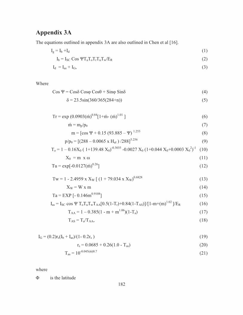
182
Appendix 3A The equations outlined in appendix 3A are also outlined in Chen et al [16].
Ig = Ib +Id (1)
Ib = ISC Cos ΨTaToTrTuTw/ER (2)
Id = Ias + IG, (3)
Where
Cos Ψ = Cosδ Cosφ Cosθ + Sinφ Sinδ (4)
δ = 23.5sin(360/365(284+n)) (5)
Tr = exp (0.0903(ḿ)0.84[1+ḿ- (ḿ)1.01 ] (6)
ḿ = mp/p0 (7)
m = [cos Ψ + 0.15 (93.885 – Ψ) 1.253 (8)
p/p0 = [(288 – 0.0065 x Hal ) /288]5.256 (9)
To = 1 – 0.16X0 ( 1+139.48 X0)-0.3035 -0.0027 X0 (1+0.044 X0+0.0003 X02)-1 (10)
X0 = m x ω (11)
Tu = exp[-0.0127(ḿ)0.26] (12)
Tw = 1 - 2.4959 x XW [ (1 + 79.034 x XW)0.6828 (13)
XW = W x m (14)
Ta = EXP [- 0.146m0.9108] (15)
Ias = ISC cos Ψ ToTuTwTAA[0.5(1-Tr)+0.84(1-TAS)]/[1-m+(m)1.02 ]/ER (16)
TAA = 1 – 0.385(1 - m + m1.06)(1-Ta) (17)
TAS = Ta/TAA, (18)
IG = (0.2)rs(Ib + Ias)/(1- 0.2rs ) (19)
rs = 0.0685 + 0.26(1.0 - Tas) (20)
Tas = 10-0.045(ḿ)0.7 (21)
where
Φ is the latitude

183
n is the Julian day
δ is the solar declination
θ is the sun hour angle (radians)
ER correction factor for the earth–sun distance Hal land surface altitude (m)
Ias atmospheric scattering of diffuse irradiance (W/m2)
Ib direct irradiance in clear sky on a horizontal surface (W/m2)
IG solar irradiance in clear sky on a horizontal surface from multiple reflections
between ground and sky (W/m2)
Ig global irradiance in clear sky on a horizontal surface (W/m2)
ISC solar constant (1366.1W/m2)
Is diffuse irradiance in clear sky on a horizontal surface (W/m2)
p0 normal atmosphere (1013 mb) Pp precipitation rate (mm/h)
Ψ solar zenith angle (in degrees)
m relative air mass
m0 pressure-corrected air mass
ω ozone amount (atm/cm)
p surface pressure in mb
p/p0 relative atmospheric pressure
Ta aerosol absorptance and Scattering transmittance
τA broadband aerosol optical depth from surface in a vertical path
TAA aerosol absorptance transmittance
TAS aerosol scattering transmittance
Tas dry air absorptance and scattering transmittance
To ozone absorption transmittance
Tr Rayleigh scattering transmittance
Tu transmittance of absorption of uniformly mixed gases (CO2 and O2)
Tw water vapor absorption transmittance
W amount of precipitable water in a vertical column from surface (cm)
X0 total amount of ozone in a slanted path (cm)
XW total amount of precipitable water in a slanted path (cm)
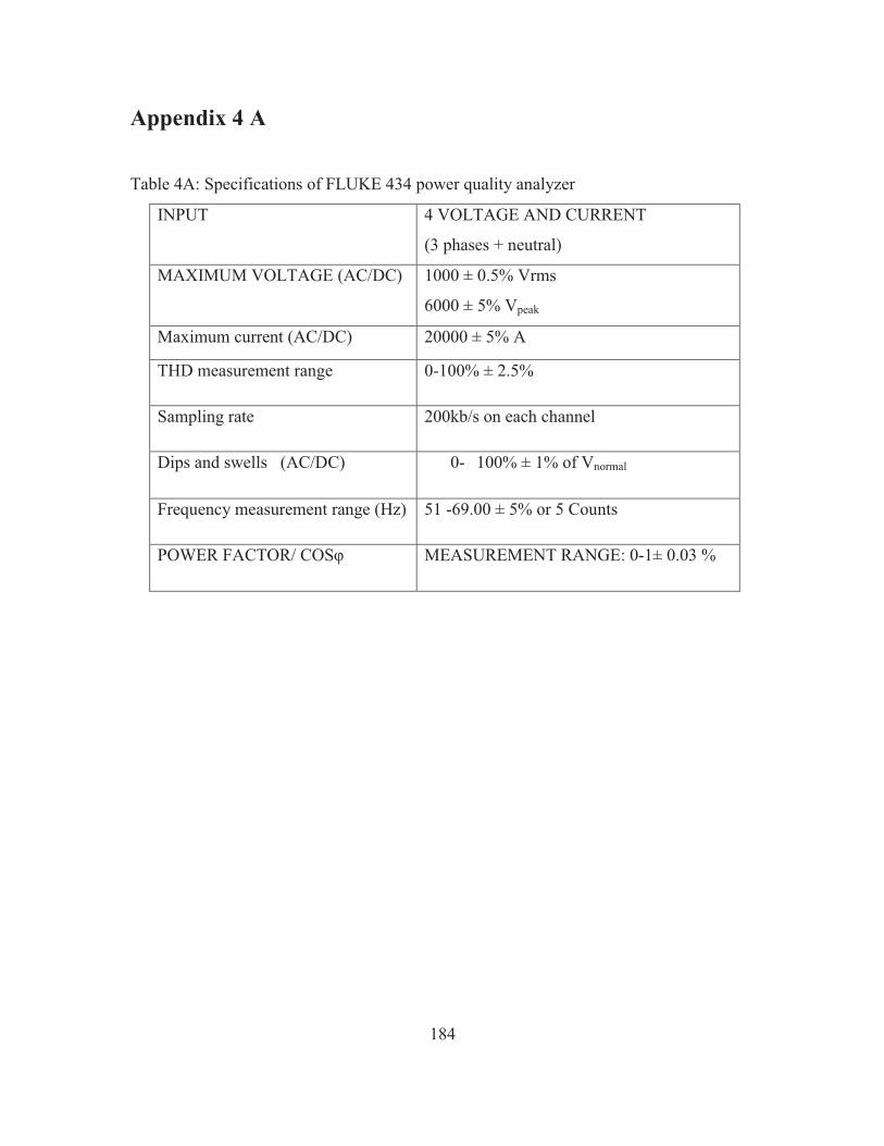
184
Appendix 4 A
Table 4A: Specifications of FLUKE 434 power quality analyzer
INPUT 4 VOLTAGE AND CURRENT
(3 phases + neutral)
MAXIMUM VOLTAGE (AC/DC) 1000 ± 0.5% Vrms
6000 ± 5% Vpeak
Maximum current (AC/DC) 20000 ± 5% A
THD measurement range 0-100% ± 2.5%
Sampling rate 200kb/s on each channel
Dips and swells (AC/DC) 0- 100% ± 1% of Vnormal
Frequency measurement range (Hz) 51 -69.00 ± 5% or 5 Counts
POWER FACTOR/ COSφ MEASUREMENT RANGE: 0-1± 0.03 %
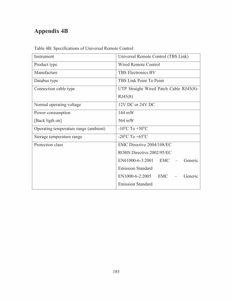
185
Appendix 4B
Table 4B: Specifications of Universal Remote Control
Instrument Universal Remote Control (TBS Link)
Product type Wired Remote Control
Manufacture TBS Electronics BV
Databus type TBS Link Point To Point
Connection cable type UTP Straight Wired Patch Cable RJ45(8)-
RJ45(8)
Normal operating voltage 12V DC or 24V DC
Power consumption
[Back ligth on]
144 mW
564 mW
Operating temperature range (ambient) -10oC To +50oC
Storage temperature range -20oC To +65oC
Protection class EMC Directive 2004/108/EC
ROHS Directive 2002/95/EC
EN61000-6-3:2001 EMC – Generic
Emission Standard
EN1000-6-2:2005 EMC – Generic
Emission Standard
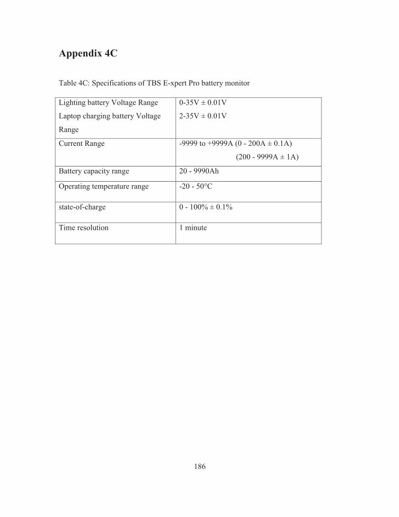
186
Appendix 4C
Table 4C: Specifications of TBS E-xpert Pro battery monitor
Lighting battery Voltage Range
Laptop charging battery Voltage
Range
0-35V ± 0.01V
2-35V ± 0.01V
Current Range
-9999 to +9999A (0 - 200A ± 0.1A)
(200 - 9999A ± 1A)
Battery capacity range 20 - 9990Ah
Operating temperature range -20 - 50°C
state-of-charge 0 - 100% ± 0.1%
Time resolution 1 minute
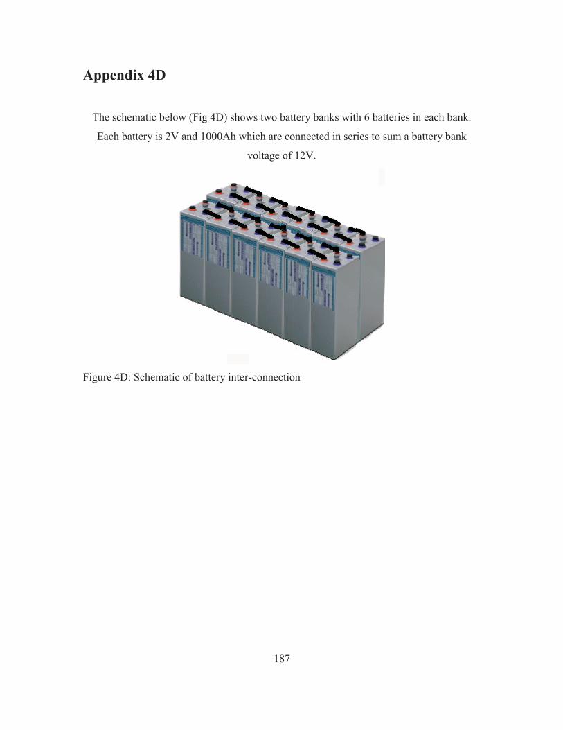
187
Appendix 4D
The schematic below (Fig 4D) shows two battery banks with 6 batteries in each bank.
Each battery is 2V and 1000Ah which are connected in series to sum a battery bank
voltage of 12V.
Figure 4D: Schematic of battery inter-connection
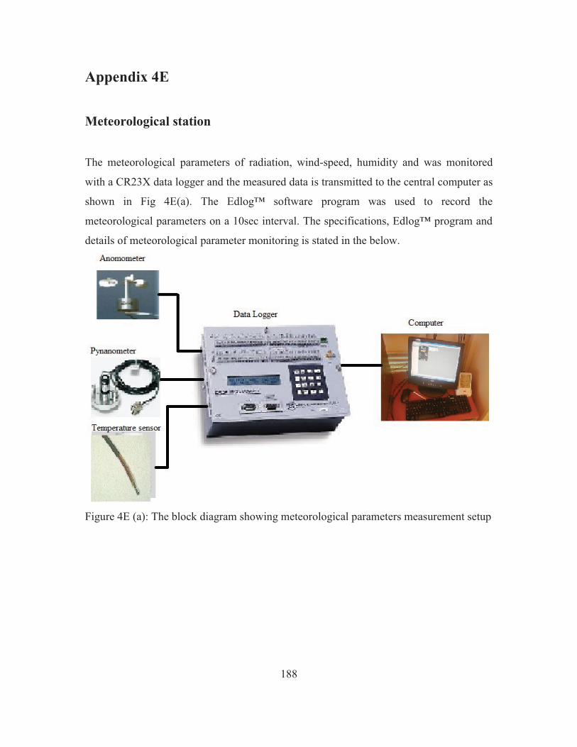
188
Appendix 4E
Meteorological station
The meteorological parameters of radiation, wind-speed, humidity and was monitored
with a CR23X data logger and the measured data is transmitted to the central computer as
shown in Fig 4E(a). The Edlog™ software program was used to record the
meteorological parameters on a 10sec interval. The specifications, Edlog™ program and
details of meteorological parameter monitoring is stated in the below.
Figure 4E (a): The block diagram showing meteorological parameters measurement setup
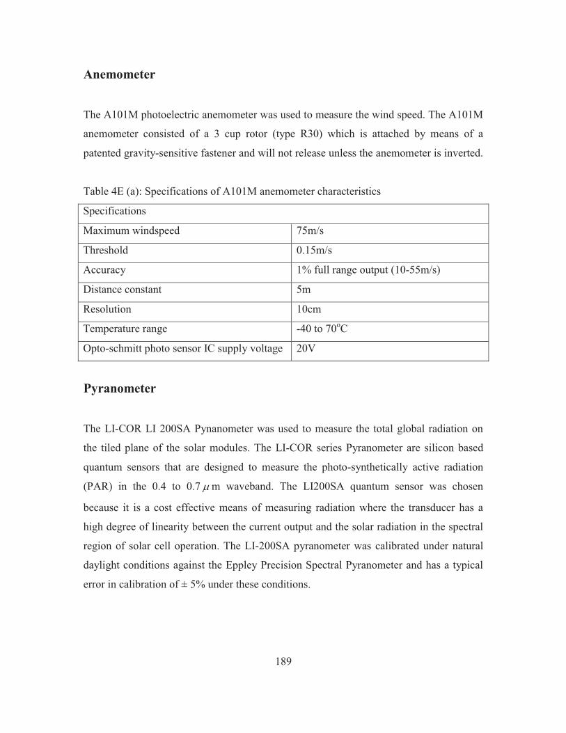
189
Anemometer
The A101M photoelectric anemometer was used to measure the wind speed. The A101M
anemometer consisted of a 3 cup rotor (type R30) which is attached by means of a
patented gravity-sensitive fastener and will not release unless the anemometer is inverted.
Table 4E (a): Specifications of A101M anemometer characteristics
Specifications
Maximum windspeed 75m/s
Threshold 0.15m/s
Accuracy 1% full range output (10-55m/s)
Distance constant 5m
Resolution 10cm
Temperature range -40 to 70oC
Opto-schmitt photo sensor IC supply voltage 20V
Pyranometer
The LI-COR LI 200SA Pynanometer was used to measure the total global radiation on
the tiled plane of the solar modules. The LI-COR series Pyranometer are silicon based
quantum sensors that are designed to measure the photo-synthetically active radiation
(PAR) in the 0.4 to 0.7 � m waveband. The LI200SA quantum sensor was chosen
because it is a cost effective means of measuring radiation where the transducer has a
high degree of linearity between the current output and the solar radiation in the spectral
region of solar cell operation. The LI-200SA pyranometer was calibrated under natural
daylight conditions against the Eppley Precision Spectral Pyranometer and has a typical
error in calibration of ± 5% under these conditions.
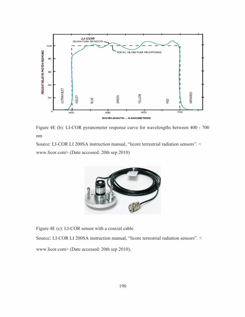
190
Figure 4E (b): LI-COR pyranometer response curve for wavelengths between 400 - 700
nm
Source: LI-COR LI 200SA instruction manual, “licore terrestrial radiation sensors”. <
www.licor.com> (Date accessed: 20th sep 2010)
Figure 4E (c): LI-COR sensor with a coaxial cable
Source: LI-COR LI 200SA instruction manual, “licore terrestrial radiation sensors”. <
www.licor.com> (Date accessed: 20th sep 2010).
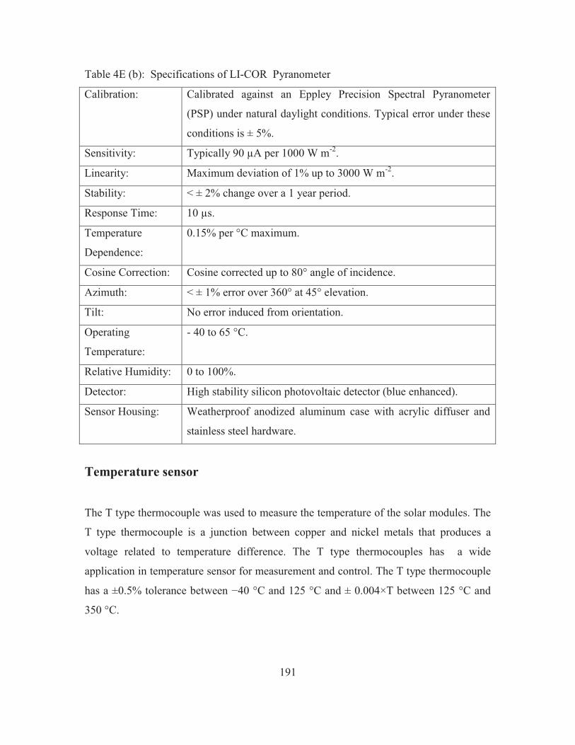
191
Table 4E (b): Specifications of LI-COR Pyranometer
Calibration: Calibrated against an Eppley Precision Spectral Pyranometer
(PSP) under natural daylight conditions. Typical error under these
conditions is ± 5%.
Sensitivity: Typically 90 μA per 1000 W m-2.
Linearity: Maximum deviation of 1% up to 3000 W m-2.
Stability: < ± 2% change over a 1 year period.
Response Time: 10 μs.
Temperature
Dependence:
0.15% per °C maximum.
Cosine Correction: Cosine corrected up to 80° angle of incidence.
Azimuth: < ± 1% error over 360° at 45° elevation.
Tilt: No error induced from orientation.
Operating
Temperature:
- 40 to 65 °C.
Relative Humidity: 0 to 100%.
Detector: High stability silicon photovoltaic detector (blue enhanced).
Sensor Housing: Weatherproof anodized aluminum case with acrylic diffuser and
stainless steel hardware.
Temperature sensor
The T type thermocouple was used to measure the temperature of the solar modules. The
T type thermocouple is a junction between copper and nickel metals that produces a
voltage related to temperature difference. The T type thermocouples has a wide
application in temperature sensor for measurement and control. The T type thermocouple
has a ±0.5% tolerance between −40 °C and 125 °C and ± 0.004×T between 125 °C and
350 °C.
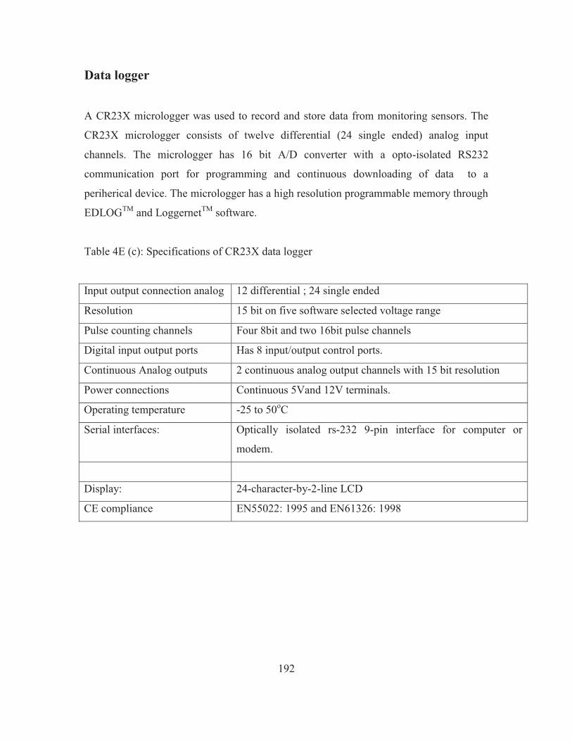
192
Data logger
A CR23X micrologger was used to record and store data from monitoring sensors. The
CR23X micrologger consists of twelve differential (24 single ended) analog input
channels. The micrologger has 16 bit A/D converter with a opto-isolated RS232
communication port for programming and continuous downloading of data to a
periherical device. The micrologger has a high resolution programmable memory through
EDLOGTM and LoggernetTM software.
Table 4E (c): Specifications of CR23X data logger
Input output connection analog 12 differential ; 24 single ended
Resolution 15 bit on five software selected voltage range
Pulse counting channels Four 8bit and two 16bit pulse channels
Digital input output ports Has 8 input/output control ports.
Continuous Analog outputs 2 continuous analog output channels with 15 bit resolution
Power connections Continuous 5Vand 12V terminals.
Operating temperature -25 to 50oC
Serial interfaces:
Optically isolated rs-232 9-pin interface for computer or
modem.
Display: 24-character-by-2-line LCD
CE compliance EN55022: 1995 and EN61326: 1998
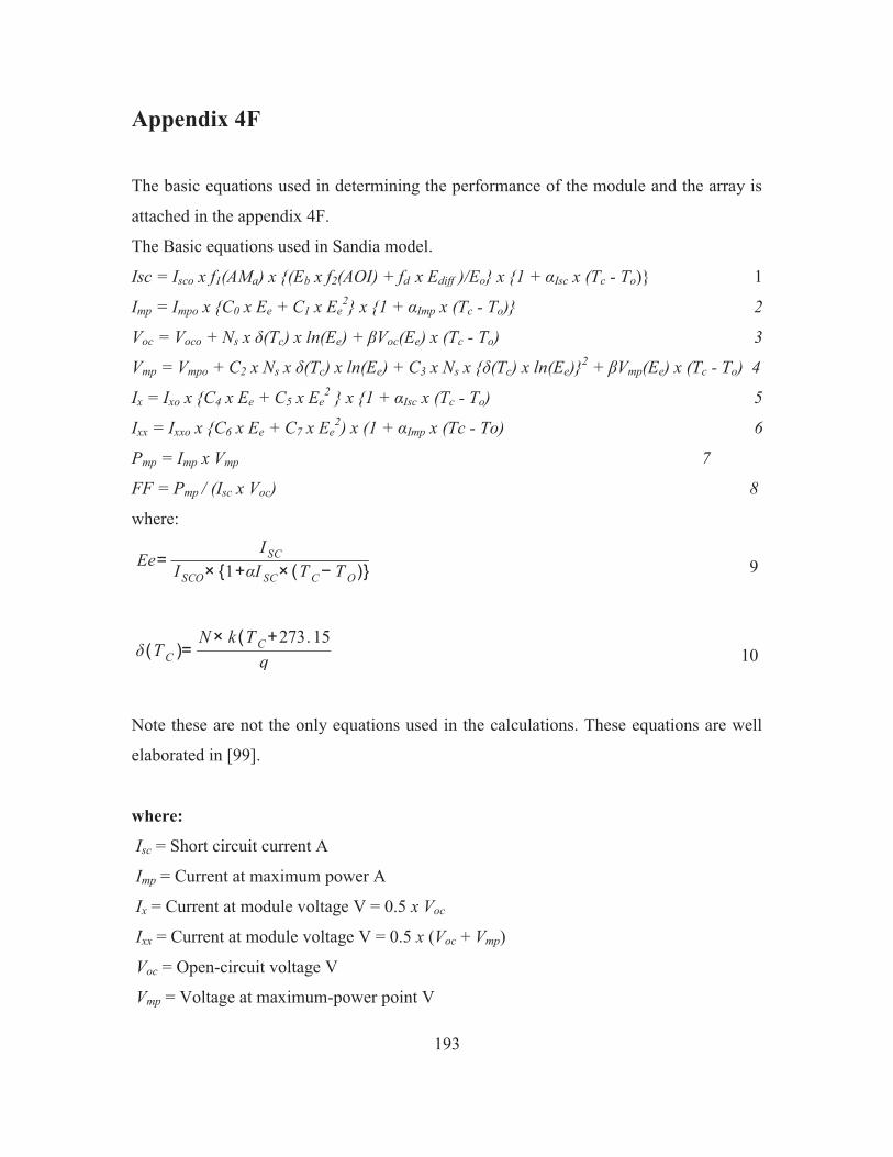
193
Appendix 4F
The basic equations used in determining the performance of the module and the array is
attached in the appendix 4F.
The Basic equations used in Sandia model.
Isc = Isco x f1(AMa) x {(Eb x f2(AOI) + fd x Ediff )/Eo} x {1 + αIsc x (Tc - To)} 1
Imp = Impo x {C0 x Ee + C1 x Ee2} x {1 + αImp x (Tc - To)} 2
Voc = Voco + Ns x δ(Tc) x ln(Ee) + βVoc(Ee) x (Tc - To) 3
Vmp = Vmpo + C2 x Ns x δ(Tc) x ln(Ee) + C3 x Ns x {δ(Tc) x ln(Ee)}2 + βVmp(Ee) x (Tc - To) 4
Ix = Ixo x {C4 x Ee + C5 x Ee2 } x {1 + αIsc x (Tc - To) 5
Ixx = Ixxo x {C6 x Ee + C7 x Ee2) x (1 + αImp x (Tc - To) 6
Pmp = Imp x Vmp 7
FF = Pmp / (Isc x Voc) 8
where:
Ee=I SC
ISCO× {1+αI SC× (T C − T O)} 9
δ(T C )=N× k (T C+273.15
q 10
Note these are not the only equations used in the calculations. These equations are well
elaborated in [99].
where:
Isc = Short circuit current A
Imp = Current at maximum power A
Ix = Current at module voltage V = 0.5 x Voc
Ixx = Current at module voltage V = 0.5 x (Voc + Vmp)
Voc = Open-circuit voltage V
Vmp = Voltage at maximum-power point V

194
Pmp = Power at maximum-power point W
FF = Fill Factor
Ns = Number of cells in series in a module's cell-string
Np = Number of cells in parallel in a module
k = Boltzmann's constant,1.38 x 1023J/K
q = Electronic charge, 1.6 x 10⁻¹⁹C
Tc = Cell temperature of the module oC
To = Reference cell temperature, typically 25oC
Eo = Reference solar irradiance, typically 1000Wm2
Ediff = Diffuse component of solar irradiance incident on the module surface, Wm2
Edni = Beam component of solar irradiance incident on the module surface, Wm2
fd = Fraction of diffuse radiation used by the cell typically 1.
AMa = Absolute air mass
αIsc = is the temperature coefficient of short circuit current variation with temperature.
%/oC
βVoc = is the temperature coefficient of open circuit voltage variation with temperature.
%/oC
αImp = is the temperature coefficient of current variation at the maximum power point
with temperature. %/oC
βVmp = is the temperature coefficient of voltage variation at the maximum power point
with temperature. %/oC
AOI = Angle of incidence. the angle between the a line perpendicular to the module
surface and the beam component of the sunlight. o
δ(Tc) = Thermal voltage per cell at temperature Tc.

195
Appendix 4G
CR23X Software Program.
The CR23X data logger was programmed with EDLOGTM software. The CR23X
program codes are given below.
CR23X program.
;{CR23X}
;* Table 1 Program
: Execution Interval ( seconds)
This instruction (P17) below, reads the reference temperature from the internal
temperature sensor and keeps latter uses this sensor as a reference junction to calculate
temperature from T type thermocouples. The datalogger stores this information in
location number 1.
;Reference Temperature
1: Panel Temperature (P17)
1: 1 -- Loc [ p_temp ]
Instruction (P2)reads the millivolt output from the pyranometer. A multiplier of 100 is
used to convert the millivolt readings into watts per square metre. The corrected radiation
value is latter stored at location number 2. The red black wires are connected to
differential channel 1,h&1 respectively. The white and clear leads was connected to an
analogue ground close to differential channel 1.
; Measure Radiation.
2: Volt (Diff) (P2)
1: 5 Reps
2: 21 10 mV, 60 Hz Reject, Slow Range
3: 1 DIFF Channel
4: 2 -- Loc [ irradan_1 ]
5: 100.0 Multiplier
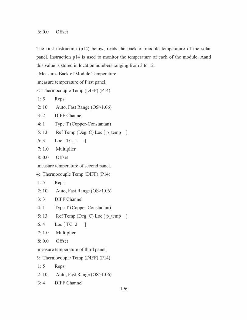
196
6: 0.0 Offset
The first instruction (p14) below, reads the back of module temperature of the solar
panel. Instruction p14 is used to monitor the temperature of each of the module. Aand
this value is stored in location numbers ranging from 3 to 12.
; Measures Back of Module Temperature.
;measure temperature of First panel.
3: Thermocouple Temp (DIFF) (P14)
1: 5 Reps
2: 10 Auto, Fast Range (OS>1.06)
3: 2 DIFF Channel
4: 1 Type T (Copper-Constantan)
5: 13 Ref Temp (Deg. C) Loc [ p_temp ]
6: 3 Loc [ TC_1 ]
7: 1.0 Multiplier
8: 0.0 Offset
;measure temperature of second panel.
4: Thermocouple Temp (DIFF) (P14)
1: 5 Reps
2: 10 Auto, Fast Range (OS>1.06)
3: 3 DIFF Channel
4: 1 Type T (Copper-Constantan)
5: 13 Ref Temp (Deg. C) Loc [ p_temp ]
6: 4 Loc [ TC_2 ]
7: 1.0 Multiplier
8: 0.0 Offset
;measure temperature of third panel.
5: Thermocouple Temp (DIFF) (P14)
1: 5 Reps
2: 10 Auto, Fast Range (OS>1.06)
3: 4 DIFF Channel
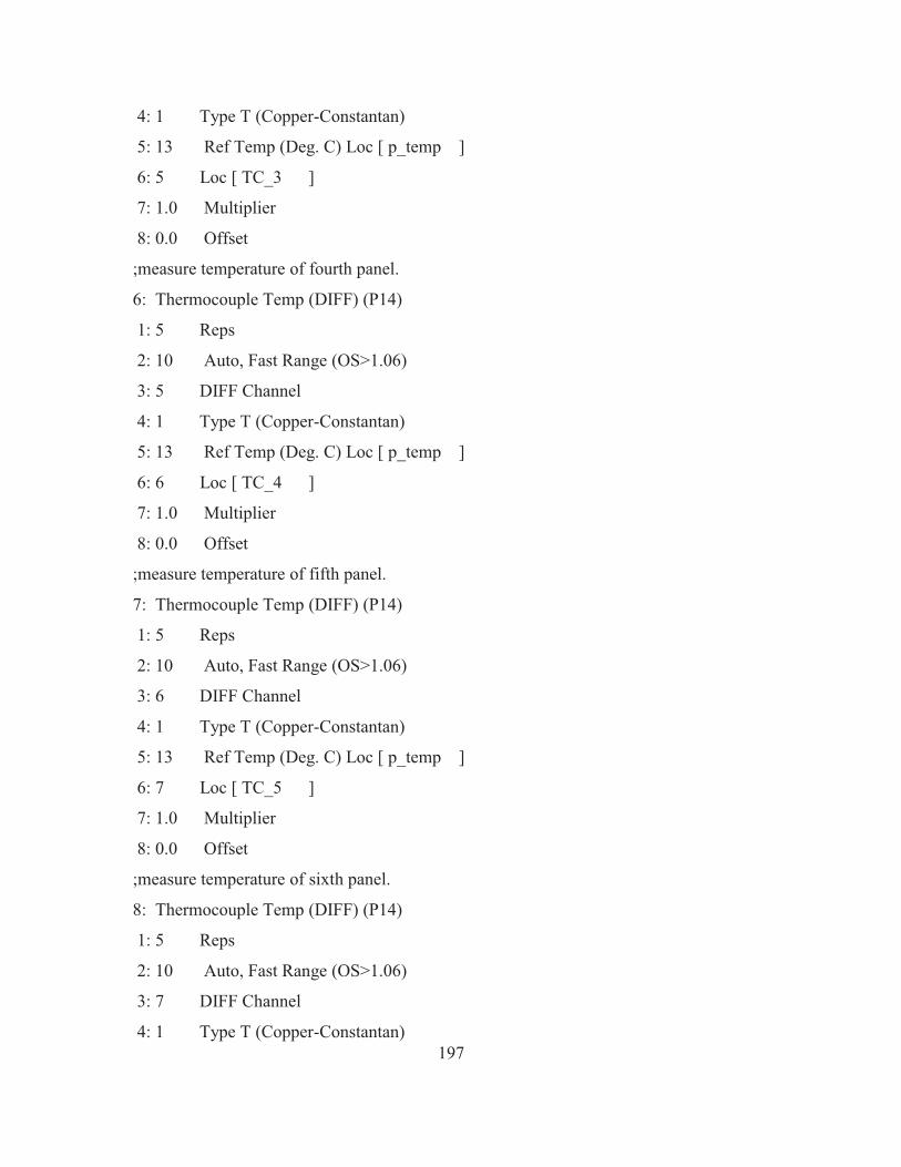
197
4: 1 Type T (Copper-Constantan)
5: 13 Ref Temp (Deg. C) Loc [ p_temp ]
6: 5 Loc [ TC_3 ]
7: 1.0 Multiplier
8: 0.0 Offset
;measure temperature of fourth panel.
6: Thermocouple Temp (DIFF) (P14)
1: 5 Reps
2: 10 Auto, Fast Range (OS>1.06)
3: 5 DIFF Channel
4: 1 Type T (Copper-Constantan)
5: 13 Ref Temp (Deg. C) Loc [ p_temp ]
6: 6 Loc [ TC_4 ]
7: 1.0 Multiplier
8: 0.0 Offset
;measure temperature of fifth panel.
7: Thermocouple Temp (DIFF) (P14)
1: 5 Reps
2: 10 Auto, Fast Range (OS>1.06)
3: 6 DIFF Channel
4: 1 Type T (Copper-Constantan)
5: 13 Ref Temp (Deg. C) Loc [ p_temp ]
6: 7 Loc [ TC_5 ]
7: 1.0 Multiplier
8: 0.0 Offset
;measure temperature of sixth panel.
8: Thermocouple Temp (DIFF) (P14)
1: 5 Reps
2: 10 Auto, Fast Range (OS>1.06)
3: 7 DIFF Channel
4: 1 Type T (Copper-Constantan)
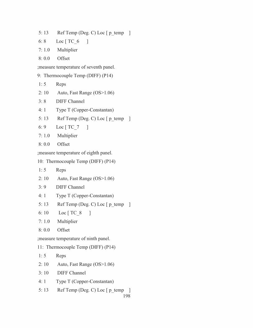
198
5: 13 Ref Temp (Deg. C) Loc [ p_temp ]
6: 8 Loc [ TC_6 ]
7: 1.0 Multiplier
8: 0.0 Offset
;measure temperature of seventh panel.
9: Thermocouple Temp (DIFF) (P14)
1: 5 Reps
2: 10 Auto, Fast Range (OS>1.06)
3: 8 DIFF Channel
4: 1 Type T (Copper-Constantan)
5: 13 Ref Temp (Deg. C) Loc [ p_temp ]
6: 9 Loc [ TC_7 ]
7: 1.0 Multiplier
8: 0.0 Offset
;measure temperature of eighth panel.
10: Thermocouple Temp (DIFF) (P14)
1: 5 Reps
2: 10 Auto, Fast Range (OS>1.06)
3: 9 DIFF Channel
4: 1 Type T (Copper-Constantan)
5: 13 Ref Temp (Deg. C) Loc [ p_temp ]
6: 10 Loc [ TC_8 ]
7: 1.0 Multiplier
8: 0.0 Offset
;measure temperature of ninth panel.
11: Thermocouple Temp (DIFF) (P14)
1: 5 Reps
2: 10 Auto, Fast Range (OS>1.06)
3: 10 DIFF Channel
4: 1 Type T (Copper-Constantan)
5: 13 Ref Temp (Deg. C) Loc [ p_temp ]
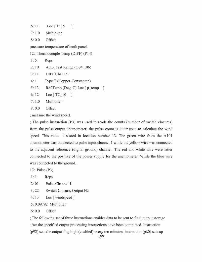
199
6: 11 Loc [ TC_9 ]
7: 1.0 Multiplier
8: 0.0 Offset
;measure temperature of tenth panel.
12: Thermocouple Temp (DIFF) (P14)
1: 5 Reps
2: 10 Auto, Fast Range (OS>1.06)
3: 11 DIFF Channel
4: 1 Type T (Copper-Constantan)
5: 13 Ref Temp (Deg. C) Loc [ p_temp ]
6: 12 Loc [ TC_10 ]
7: 1.0 Multiplier
8: 0.0 Offset
; measure the wind speed.
; The pulse instruction (P3) was used to reads the counts (number of switch closures)
from the pulse output anemometer, the pulse count is latter used to calculate the wind
speed. This value is stored in location number 13. The green wire from the A101
anemometer was connected to pulse input channel 1 while the yellow wire was connected
to the adjacent reference (digital ground) channel. The red and white wire were latter
connected to the positive of the power supply for the anemometer. While the blue wire
was connected to the ground.
13: Pulse (P3)
1: 1 Reps
2: 01 Pulse Channel 1
3: 22 Switch Closure, Output Hz
4: 13 Loc [ windspeed ]
5: 0.09792 Multiplier
6: 0.0 Offset
; The following set of three instructions enables data to be sent to final output storage
after the specified output processing instructions have been completed. Instruction
(p92) sets the output flag high (enabled) every ten minutes, instruction (p80) sets up
200
a data array named '111' in final storage area 1. Instruction (p77) timestamps all data
sets that are being sent to the output array.
14: If time is (P92)
1: 0 -- Minutes (Seconds --) into a
2: 10 -- Interval (same units as above)
3: 10 Set Output Flag High (Flag 0)
15: Set Active Storage Area (P80)^31508
1: 1 Final Storage Area 1
2: 111 Array ID
16: Real Time (P77)^7083
1: 1221 Year,Day,Hour/Minute,Seconds (midnight = 2400)
17: Average (P71)
1: 13 Reps
2: 3 Loc [ TC_1 ]
This last instruction enables automatic data transfer to data storage device if it is
connected via the serial i/o port to the computer.
18: Serial Out (P96)
1: 42 Destination Output
8 Table 2 Program
: Execution Interval (seconds)
* Table 3 Subroutines
End Program
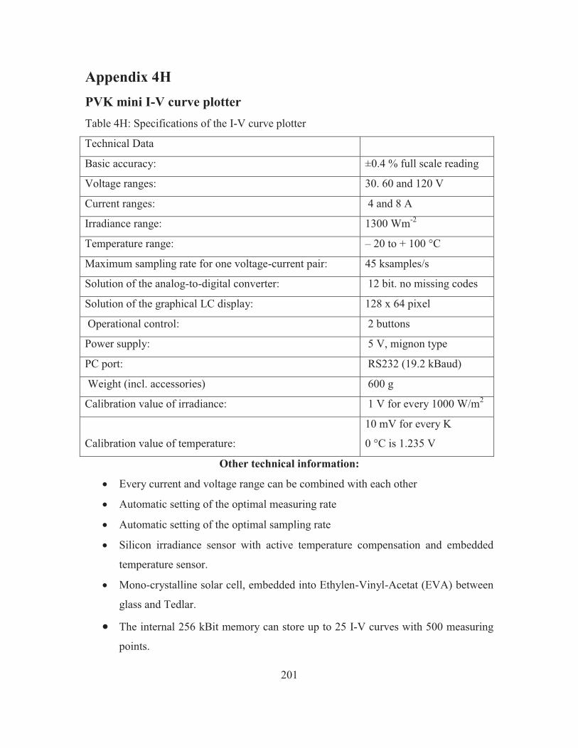
201
Appendix 4H PVK mini I-V curve plotter Table 4H: Specifications of the I-V curve plotter
Technical Data
Basic accuracy: ±0.4 % full scale reading
Voltage ranges: 30. 60 and 120 V
Current ranges: 4 and 8 A
Irradiance range: 1300 Wm-2
Temperature range: – 20 to + 100 °C
Maximum sampling rate for one voltage-current pair: 45 ksamples/s
Solution of the analog-to-digital converter: 12 bit. no missing codes
Solution of the graphical LC display: 128 x 64 pixel
Operational control: 2 buttons
Power supply: 5 V, mignon type
PC port: RS232 (19.2 kBaud)
Weight (incl. accessories) 600 g
Calibration value of irradiance: 1 V for every 1000 W/m2
Calibration value of temperature:
10 mV for every K
0 °C is 1.235 V
Other technical information:
� Every current and voltage range can be combined with each other
� Automatic setting of the optimal measuring rate
� Automatic setting of the optimal sampling rate
� Silicon irradiance sensor with active temperature compensation and embedded
temperature sensor.
� Mono-crystalline solar cell, embedded into Ethylen-Vinyl-Acetat (EVA) between
glass and Tedlar.
� The internal 256 kBit memory can store up to 25 I-V curves with 500 measuring
points.
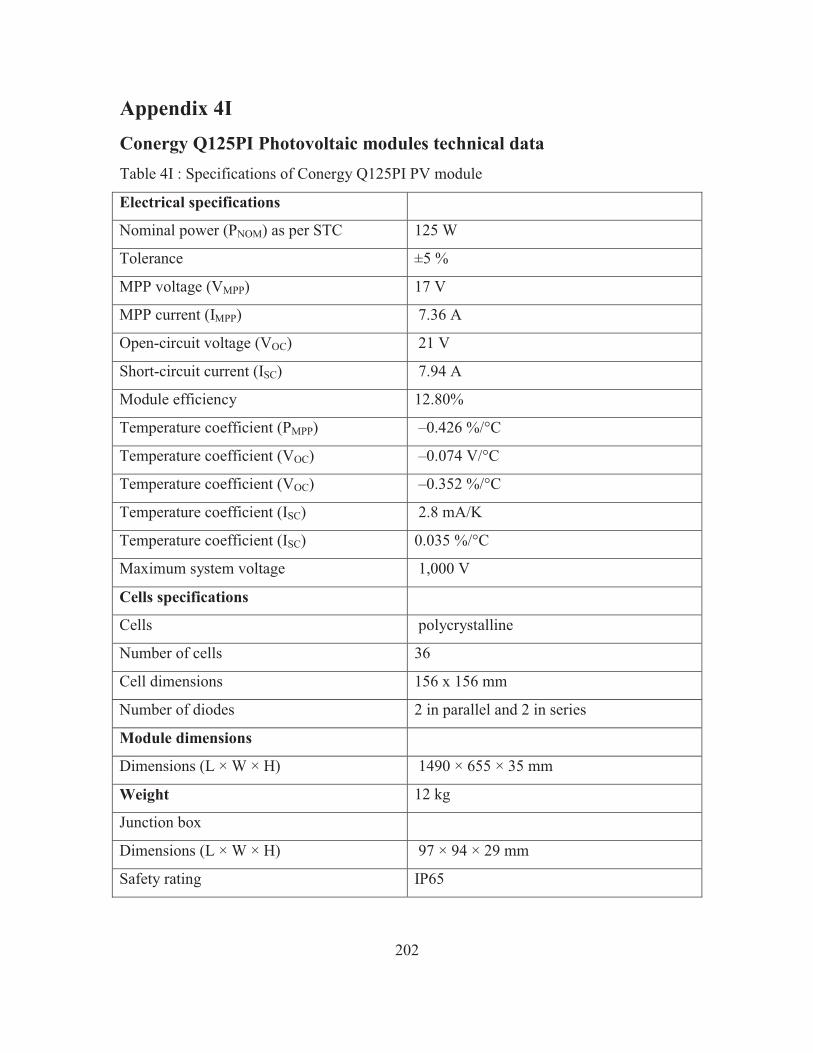
202
Appendix 4I Conergy Q125PI Photovoltaic modules technical data Table 4I : Specifications of Conergy Q125PI PV module
Electrical specifications
Nominal power (PNOM) as per STC 125 W
Tolerance ±5 %
MPP voltage (VMPP) 17 V
MPP current (IMPP) 7.36 A
Open-circuit voltage (VOC) 21 V
Short-circuit current (ISC) 7.94 A
Module efficiency 12.80%
Temperature coefficient (PMPP) –0.426 %/°C
Temperature coefficient (VOC) –0.074 V/°C
Temperature coefficient (VOC) –0.352 %/°C
Temperature coefficient (ISC) 2.8 mA/K
Temperature coefficient (ISC) 0.035 %/°C
Maximum system voltage 1,000 V
Cells specifications
Cells polycrystalline
Number of cells 36
Cell dimensions 156 x 156 mm
Number of diodes 2 in parallel and 2 in series
Module dimensions
Dimensions (L × W × H) 1490 × 655 × 35 mm
Weight 12 kg
Junction box
Dimensions (L × W × H) 97 × 94 × 29 mm
Safety rating IP65

203


![170321 Eichner AAPV-SAPV WS-1.ppt [Kompatibilitätsmodus] · (E. Eichner 2010, phil. Dissertation, noch unveröffentlicht ) Verordnung von SAPV Dr. Eckhard Eichner Augsburger Hospiz-und](https://img.pdfslide.net/doc/110x75/60609454bd5cd41a4c0b187b/170321-eichner-aapv-sapv-ws-1ppt-kompatibilittsmodus-e-eichner-2010-phil.jpg)