780 Vehicle physics

Equations for v in m/s Equations for v in km/h

Acceleration or braking (deceleration) in m/s2 a-£-.!:-E-2s-I-(2

a_~__V_-E - 26 s - 3.6 t - 12

Acceleration or braking time in s

t-.!:-E-{ii-a-V-{l I = 3.~a = 7:; s = {ii

Accelerating or braking distance inm

v2 vi al 2 s=2l1=2= -2­

V2 VI al 2 s= 26a =7.2 =--y

Motor-vehicle dynamics 781

Tables 9 and 10 exist between the gra­dient angle a, coefficient of static friction Pr and maximum acceleration or decel­eration. The real-world figures are always somewhat lower, as all the vehicle's tires do not simultaneously exploit their maxi­mum adhesion during each acceleration or deceleration. Electronic traction control and braking systems (TCS, ABS, ESP) maintain the traction level in the vicinity of the coefficient of static friction.

k indicates the ratio between the load on driven or braked wheels and the total weight. If all wheels are driven or braked, Ie = 1. At 50% load distribution k = 0.5.

Example:

k = 0.5; g = 10 m/s2; Pr=0.6;p = 15%; ({max = 10·(0.5·0.6 ± 0.15) m/s2 upgrade braking (+): amax = 4.5 m/s2, downgrade braking (-): amax = 1.5 m/s2.

Work and power The power required to maintain a con­sistent rate of acceleration (decelera­tion) varies according to vehicle speed (Table 11). The power available for ac­celeration is:

Pa = P 1] - Pw, where

P Engine output 1] Efficiency Pw Motive power

Actions: Reaction, braking and stopping (in accordance with ONORM V 5050 [1] and [2])

Hazard recognition time The hazard recognition time, also known as the danger reaction time, is the period of time that elapses between perceiving a visible obstacle or its movement and the time required to recognize it as a hazard (Figure 6). If, as part of this dan­ger recognition and response process, it is necessary for the driver to turn his

eyes towards the hazardous situation, the hazard recognition and danger reaction time will extend by roughly 0.4 s.

Prebraking time The prebraking time (tvz) is the period of time that elapses between the moment the hazard is recognized and the start of braking, defined by way of calculation. Based on the following formula, the pre­braking time is in the range from approx. 0.8 to 1.0 s:

tvz = tR + lu + tA + Is 12 .

The reaction time (tR) is the period of time that elapses between the moment a defined incitement to action occurs and the start of the first specifically targeted action. Instinctive hazard recognition triggers an inherent, automatic reaction (spontaneous reaction), enabling the vehicle driver to determine both the point of the reaction as well as the position of the reason for the reaction, delayed by the distance covered during the prebraking time. Human beings require about 0.2 s for the spontaneous reaction; however, the reaction time will be at least 0.3s if the driver needs to make a decision to perform a preventive or evasive action in response to conscious hazard recognition (choice reaction) .

The transfer time (tu) is the period of time the driver requires to transfer the foot from the accelerator pedal to the brake pedal. The transfer time is in the range of about 0.2 s.

The response time (tA) is the period of time it takes to transmit the pressure applied at the brake pedal via the brake system through to the point when the braking action becomes effective (com­plete build-up of the application force and incipient increase in vehicle deceleration).

The pressure build-up time (ts) is the period of time that elapses between the braking action taking effect and reaching fully effective braking deceleration. Alter­natively, half the pressure build-up time (tsf2) may be assumed as the start of braking, determined by way of calculation.

In accordance with the EU Council of Ministers Directive EEC 71/320 Adden­dum 312.4 [3], the sum of the response

which a layer of water separates the tire and the (wet) road surface (Figure 5) . The phenomenon occurs when a wedge of water forces its way underneath the tire's contact patch and lifts it from the road . The tendency to aquaplane is dependent upon such factors as the depth of the water on the road surface, the vehicle's speed, the tread pattern, the tread wear, and the load pressing the tire against the road surface. Wide tires are particularly susceptible to aquaplaning. An aquaplaning vehicle can­not transmit control and braking forces to the road surface, and may as result go into a skid.

Table 8: Accelerating and braking

Table 9: Acceleration and braking (deceleration)

Accelerating and braking

The vehicle is regarded as accelerating or braking (decelerating) at a constant rate when 0. remains constant. The equations set out in Table 8 apply to an initial or final speed of v =O.

Maxima for acceleration and braking (deceleration) When the motive or braking forces exerted at the vehicle's wheels reach such a mag­nitude that the tires are just still within their limit of adhesion (maximum adhesion is still present), the relationships shown in

Level road surface

Inclined road surface anp=100tana[%]

Limit acceleration or deceleration am" in m/s2

amax = kgp, am" =g (kPr cosa±sina) approximation ': amlJJ< "'g (kPr ±0.01p)

+when upgrade braking or downgrade acceleration

-when upgrade acceleration or downgrade braking

1

Level road surface Inclined road surface

+ Downgrade acceleration 3,600 Pa -Upgrade accelerationa. = 3,600 Pa ± g sin aa --- ­

e - kmv kmv for g sin a the approximation 1

gpl100

Table 10: Achievable acceleration a. (Pa in kW, v in km/h, 111 in kg)

Table 11: Work and power

Level Inclined road surface road surface a [oJ;P = 100 tan a [%J

Acceleration or W=kmas W=ms(ka±gsina) + Downgrade braking Braking work W approximation 1: or upgrade acceleration in J2 W= ms (ka ± gp1100) -Downgrade acceleration

or upgrade braking Acceleration or Pa = kmasv Pa = m v (ka ± g sin a) braking power in W approximation ': v in m/s. For v in km/h, at velocity v Pa=mv(ka±gpI100) use vI3.6.

1 Valid to approx.p=20% (under 2% error), 21 J = 1 N m = 1 W s.

782 Vehicle physics

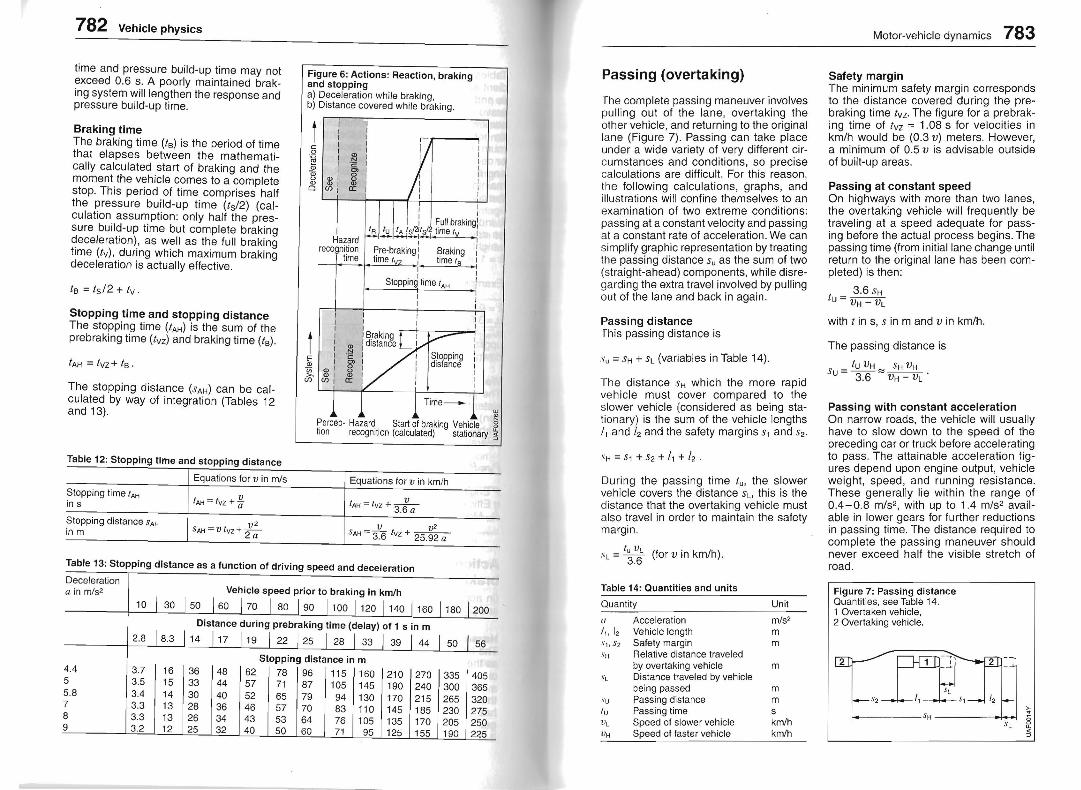
time and pressure build-up time may not exceed 0.6 s. A poorly maintained brak­ing system will lengthen the response and pressure build-up time.

Braking time The braking time (Is) is the period of time that elapses between the mathemati­cally calculated start of braking and the moment the vehicle comes to a complete stop. This period of time comprises half the pressure build-up time (tsl2) (cal­culation assumption: only half the pres­sure build-up time but complete braking deceleration), as well as the full braking time (tv), during which maximum braking deceleration is actually effective.

IB =ts/2 + tv.

Stopping time and stopping distance The stopping time (tAH) is the sum of the prebraking time (tvz) and braking time (ts) .

tAH = tvz+ tB .

The stopping distance (SAH) can be cal­culated by way of integration (Tables 12 and 13).

Table 12: Stopping time and stopping distance

Figure 6: Actions: Reaction, braking and stopping a) Deceleration while braking, b) Distance covered while braking.

t

, ' , ' , Full braking:

I tA 151211512 lime Iv , Hazard J~' -I

recognition Pre·braking' Braking : time time I z : time 18 '

I - I I

Stopping' time IAH : I, I

t E Q)

~ ~ (/) (/)

Percep· Hazard Start of braking Vehicle tion recognition (calculated) stationary

Table 13: Stopping distance as a function of driving speed and deceleration

Deceleration a in m/s2

10 I 30

Vehicle speed prior to braking in km/h

150 160 170 '1 80 190 1100 J120 1140 1160 1180 1200

2.8 18.3

Distance during prebraking time (delay) of 1 s in m

114 117 119 J 22 J25 I 28 I 33 I 39 1 44 I 50 I 56

4.4 5 5.8 7 8 9

3.7 16 3.5 15 3.4 14 3.3 13 3.3 13 3.2 12

Stopping distance in m 36 48 62 78 96 115 160 210 270 33 44 57 71 87 105 145 190 240 30 40 52 65 79 1:)4 130 170 215 28 36 46 57 70 83 110 145 185 26 34 43 53 64 76 105 135 170 25 32 40 50 60 71 95 125 155

335 300 265 230 205

405 365 320 275 250

Motor-vehicle dynamics 783

Passing (overtaking)

fhe complete passing maneuver involves pulling out of the lane, overtaking the other vehicle, and returning to the original lane (Figure 7). Passing can take place under a wide variety of very different cir­cumstances and conditions, so precise calculations are difficult. For this reason, the following calculations, graphs, and illustrations will confine themselves to an examination of two extreme conditions: passing at a constant velocity and passing at a constant rate of acceleration. We can simplify graphic representation by treating tI1e passing distance Su as the sum of two (straight-ahead) components, while disre­garding the extra travel involved by pulling out of the lane and back in again .

Passing distance fhis passing distance is

Su = SH + SL (variables in Table 14).

The distance SH which the more rapid vehicle must cover compared to the slower vehicle (considered as being sta­tionary) is the sum of the vehicle lengths I, and 12 and the safety margins S1 and h

During the passing time lu, the slower vehicle covers the distance SL, this is the distance that the overtaking vehicle must also travel in order to maintain the safety margin.

IL = t3v~ (for v in km/h) .

Table 14: Quantities and units

Quantity Unit

(/

I" 12 -'" \ ,S2

,\'H

·\'L

Xu lu

V L

VH

Acceleration Vehicle length Safety margin Relative distance traveled by overtaking vehicle Distance traveled by vehicle being passed Passing distance Passing time Speed of slower vehicle Speed of faster vehicle

m/s2

m m

m

m m s km/h km/h

Safety margin The minimum safety margin corresponds to the distance covered during the pre­braking time tvz. The figure for a prebrak­ing time of tvz = 1.08 s for velocities in km/h would be (0.3 v) meters. However, a minimum of 0.5 v is advisable outside of built-up areas.

Passing at constant speed On highways with more than two lanes, the overtaking vehicle will frequently be traveling at a speed adequate for pass­ing before the actual process begins. The passing time (from initial lane change until return to the original lane has been com­pleted) is then:

t _ 3.6 SH u - VH - VL

with t in s, s in m and v in km/h.

The passing distance is

tu VH SH VH Su =3.6 '" VH - VL .

Passing with constant acceleration On narrow roads, the vehicle will usually have to slow down to the speed of the preceding car or truck before accelerating to pass. The attainable acceleration fig­ures depend upon engine output, vehicle weight, speed, and running resistance. These generally lie within the range of 0.4-0.8 m/s2, with up to 1.4 m/s2 avail­able in lower gears for further reductions in passing time. The distance required to complete the passing maneuver should never exceed half the visible stretch of road.

Figure 7: Passing distance Quantities, see Table 14. 1 Overtaken vehicle, 2 Overtaking vehicle.

~-------- SH---------'~

Equations for v in mls

Stopping time tAH tAH = tvz + *in 5

Stopping distance SAH V2 in m SAH =v/vz+ 2Q

Equations for v in kml h

tAH = tvz + _v_3.6 a

v v2 SAH= 3.6 /vz + 25.92 a

190 225

784 Vehicle physics

Operating on the assumption that a constant rate of acceleration can be maintained for the duration of the passing maneuver, the passing time will be:

tu = hswa . The distance which the slower vehicle covers within this period is defined as SL = tuvL/3 .6. This gives a passing dis­tance of:

tUVL Su= SH+ 3.6 .

with t in s, S in m and v in km/h.

The left side of Figure 8 shows the rela­tive distances SH for speed differentials VH-VL and acceleration rates a, while the right side shows the distances SL covered by the vehicle being passed at various speeds VL. The passing distance Su is the sum of SH and SL.

First, determine the distance SH to be traveled by the passing vehicle. Enter this distance on the left side of the graph between the Y axis and the applicable (vH-vLl line or acceleration line. Then extrapolate the line to the right, over to the speed line VL.

Figure 8: Graph for determining passing distance

ReI. distance SH traveled by passing vehicle Distance SL traveled by vehicle being passed

100 63 40 25 16 10 10 16 25 40 63 100 160 250400 m

0.4 50 '31.5

1

80

~

~

~ .'" ~~ I"> "" '" I">

I<:--~

I

,'I-,j ~ ' r-

-~ N " '" ~ !'-'

20 12.5 12.5 20 31 .5 50

1- . .[- ' 1- . 1- """' -- -- -- -- -- . .., - r..,

I"-~ l"-

I<:-- l" I"-~ ~

10/

12.5 V

16 20

25 IT?",.! " ,,31.5 / / / / /

80 1125 I 200 315

' 1"- .~ - ' -;

F"7 r7 -j

s 20

.Q ~ 0,63

16 "§ 1.6 12.5 '" ~ m/s2 10 .: :}, '" 8 ~

6.3 OJ

5 .~

4 rf'" 3.15 2.5 2 1.6 1.25 1

km/h 80 635040 40 50 63 80 100 km/h

Example (represented by dash-dot lines in the graph): VL =VH =50 km/h, a = 0.4 m/s2, 11 = 10m, 12 = 5 m, SI = S2 = 0.3 VL = 0.3 VH =15 m.

Solution: Enter intersection of a = 0.4 m/s2 and SH = 15 + 15 + 1 0 + 5 = 45 m in the left side of the graph. Indication: tu = 5 S, SL = 210m. The following applies: Su = SH + SL = 255 m.

Visual range For safe passing on narrow roads, the visibility must be at least the sum of the passing distance plus the distance which would be traveled by an oncoming vehicle while the passing maneuver is in prog­ress . This distance is approximately 400 m if the vehicles approaching each other are traveling at speeds of 90 km/h, and the vehicle being overtaken at 60 km/h.

Motor-vehicle dynamics 785

Fuel consumption

Determining fuel consumption The official data for standard fuel con­sumption are determined on the basis of dynamometer tests conducted on ex­haust-emission test benches in which tatutory test cycles (e.g. MNEDC for

Europe, FTP75 and Highway for the USA and JC08 for Japan) are run . The exhaust gas is collected in sample bags and its constituents HC, CO and CO2 are subse­quently analyzed for the purpose of deter­mining consumption (see Exhaust-gas measuring techniques) . The CO2 content of the exhaust gas is proportional to the fuel consumption.

The following reference values apply to Europe: Diesel: 1 l/100km '" 26.5 g C02/km . Gasoline (Euro 4):

1 l/100km '" 24.0 g C02/km. Gasoline (Euro 5):

1 l/100km '" 23.4 g C02/km.

The change from Euro 4 to Euro 5 is based on a 5% admixture of ethanol in gasoline.

Figure 9: Effect of vehicle design on fuel consumption Quantities, see Table 15.

Vehicle weights are simulated on the test bench as an alternative by test weights which, depending on the country and the curb weight of the vehicle, is graded in increments of 55-120 kg. When the vehicle weight is allocated to the corre­sponding inertia weight class, the ready­for-operation weight of the vehicle (including all the fillers, tool kit and the fuel

Table 15: Quantities and units

Quantity Unit

B. Distance consumption g/m b. Specific fuel consumption g/kWh In Vehicle mass kg A Frontal area of vehicle m2

I Coefficient of rolling resistance -Cd Drag coefficient g Gravitational acceleration m/s2

t Time s v Driving speed m/s a Acceleration m/S2 B, Braking resistance N

710 Transmission efficiency of drivetrain

p Density of the air kg/m3

a Gradient angle 0

Consumption per ......1-------- Fuel consumption ---------l.~ unit of distance

Drivetrain ......b------ Resistance factors ----------l.~

Engine Rolling resistance Aerodynamic drag Acceleration resistance

Climbing resistance

Braking resistance

I ;be·+u-[ (m I g' cosa+~. cw ' A ,v2 ) + m(a + g' sina) + Br j·v. dt

Be= v · dt

I DistanceSpeed VL