Embed Size (px)
DESCRIPTION
Frank White Fluid Mechanics 7th Ed. Ch. 4 Solutions
Citation preview

Chapter 4 Differential Relations for a Fluid Particle
P4.1 An idealized velocity field is given by the formula
24 2 4tx t y xz V i j k
Is this flow field steady or unsteady? Is it two- or three-dimensional? At the point (x, y, z) (–1, 1, 0), compute (a) the acceleration vector and (b) any unit vector normal to the acceleration.
Solution: (a) The flow is unsteady because time t appears explicitly in the components. (b) The flow is three-dimensional because all three velocity components are nonzero. (c) Evaluate, by laborious differentiation, the acceleration vector at (x, y, z) (1, 1, 0).
2 2
2 2 4
2 2
du u u u uu v w 4x 4tx(4t) 2t y(0) 4xz(0) 4x 16t x
dt t x y z
dv v v v vu v w 4ty 4tx(0) 2t y( 2t ) 4xz(0) 4ty 4t y
dt t x y z
dw w w w wu v w 0 4tx(4z) 2t y(0) 4xz(4x) 16txz 16x z
dt t x y z
2 4 2dor: (4x 16t x) ( 4ty 4t y) (16txz 16x z)
dt
Vi j k
at (x, y, z) (1, 1, 0), we obtain 2 3d4(1 4t ) 4t(1 t ) 0 (c)
dtAns.
Vi j k
(d) At (–1, 1, 0) there are many unit vectors normal to dV/dt. One obvious one is k. Ans.
P4.2 Flow through the converging nozzle in Fig. P4.2 can be approximated by the one-dimensional velocity distribution
o2
1 0 0x
u V wL
(a) Find a general expression for the fluid acceleration in the nozzle. (b) For the specific case Vo 10 ft/s and L 6 in, compute the acceleration, in g’s, at the entrance and at the exit.
Fig. P4.2
Chapter 4 Differential Relations for a Fluid Particle 303
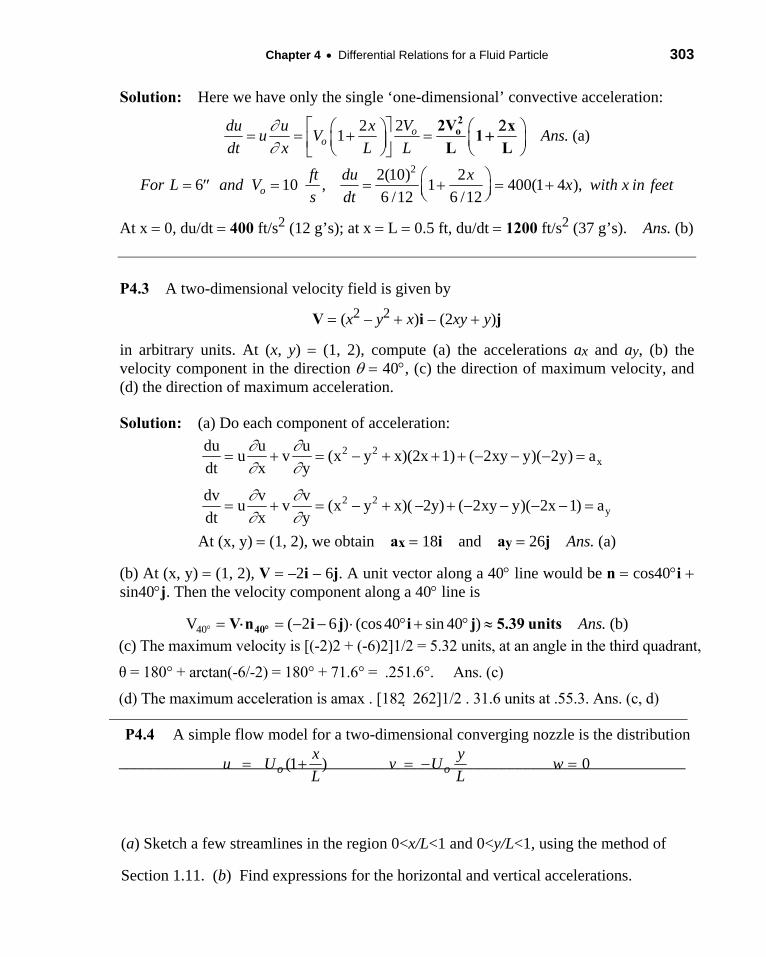
Solution: Here we have only the single ‘one-dimensional’ convective acceleration:
221 . (a)o
oVdu u x
u V Ansdt x L L
2o2V x
1L L
22(10) 2 6 10 , 1 400(1 4 ),
6 /12 6 /12oft du x
For L and V x with x in feets dt
At x 0, du/dt 400 ft/s2 (12 g’s); at x L 0.5 ft, du/dt 1200 ft/s2 (37 g’s). Ans. (b)
P4.3 A two-dimensional velocity field is given by
V (x2 – y2 x)i – (2xy y)j
in arbitrary units. At (x, y) (1, 2), compute (a) the accelerations ax and ay, (b) the velocity component in the direction 40, (c) the direction of maximum velocity, and (d) the direction of maximum acceleration.
Solution: (a) Do each component of acceleration:
2 2x
2 2y
du u uu v (x y x)(2x 1) ( 2xy y)( 2y) a
dt x y
dv v vu v (x y x)( 2y) ( 2xy y)( 2x 1) a
dt x y
At (x, y) (1, 2), we obtain ax 18i and ay 26j Ans. (a)
(b) At (x, y) (1, 2), V –2i – 6j. A unit vector along a 40 line would be n cos40i sin40j. Then the velocity component along a 40 line is
40V ( 2 6 ) (cos 40 sin 40 ) . (b)Ans 40V n i j i j 5.39 units
(c) The maximum velocity is [(-2)2 + (-6)2]1/2 = 5.32 units, at an angle in the third quadrant,
θ = 180° + arctan(-6/-2) = 180° + 71.6° = .251.6°. Ans. (c)
(d) The maximum acceleration is amax . [182 262]1/2 . 31.6 units at .55.3. Ans. (c, d)
_______________________________________________________________________
P4.4 A simple flow model for a two-dimensional converging nozzle is the distribution
(a) Sketch a few streamlines in the region 0<x/L<1 and 0<y/L<1, using the method of
Section 1.11. (b) Find expressions for the horizontal and vertical accelerations.
0)1( wL
yUv
L
xUu oo
Solutions Manual Fluid Mechanics, Fifth Edition
304
(c) Where is the largest resultant acceleration and its numerical value?
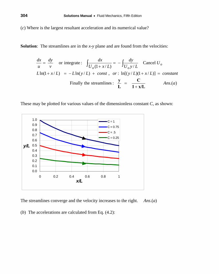
Solution: The streamlines are in the x-y plane and are found from the velocities:
These may be plotted for various values of the dimensionless constant C, as shown:
0.0
0.1
0.2
0.3
0.4
0.5
0.6
0.7
0.8
0.9
1.0
0 0.2 0.4 0.6 0.8 1
x/L
y/L
C = 1
C = 0.75
C = .5
C = 0.25
The streamlines converge and the velocity increases to the right. Ans.(a)
(b) The accelerations are calculated from Eq. (4.2):
).(:sstreamlinetheFinally
)]/1)(/ln[(:,)/ln()/1ln(
Cancel/)/1(
:integrateor
aAns
constantLxLyorconstLyLLxL
ULyU
dy
LxU
dx
v
dy
u
dxo
oo
x/L1
C
L
y
Chapter 4 Differential Relations for a Fluid Particle 305
(c) Find the resultant of ax and ay from Ans.(b) above and introduce y/L from Ans.(a):
2 2 2 2 21 2 /(1 ) , where / .( )x ya a a C x L Ans c
We observe that the resultant acceleration increases with x and is greatest at x = L, where its
numerical value is (Uo2/L) [4 + C2/4]1/2.
P4.5 The velocity field near a stagnation point (see Example 1.10) may be written in the form
o o
ou v and are constantsU x U y
U LL L
(a) Show that the acceleration vector is purely radial. (b) For the particular case L 1.5 m, if the acceleration at (x, y) (1 m, 1 m) is 25 m/s2, what is the value of Uo?
Solution: (a) For two-dimensional steady flow, the acceleration components are
2o o
o o 2
2o o
o o 2
U Udu u u x yu v U U (0) x
dt x y L L L L
U Udv v v x yu v U (0) U y
dt x y L L L L
Therefore the resultant 2 2 2 2o o(U /L )(x y ) (U /L (purely radial) (a)Ans. a i j )r
(b) For the given resultant acceleration of 25 m/s2 at (x, y) (1 m, 1 m), we obtain
2 2o o
o2 2 2
U Um ra 25 2 m, solve for U . (b)s L (1.5 m)
Ans m
6.3s
).()/)(/(0
)1(0)/)](/1([
2
2
bAnsL
y
L
ULULyU
y
vv
x
vua
L
x
L
ULULxU
y
uv
x
uua
oooy
ooox
Solutions Manual Fluid Mechanics, Fifth Edition
306
P4.6 An incompressible plane flow has the velocity components u = 2y, v = 8x, w = 0. (a) Find the acceleration components. (b) Determine if the vector acceleration is radial.
(c) Which two streamlines of this flow are straight lines?
Solution: (a, b) With no z activity, we can stick to steady two-dimensional formulas:
(2 )(0) (8 )(2) 16
(2 )(8) (8 )(0) 16 .( )
16 16 16( ) 16 , yes. .( )
x
y
x y
u ua u v y x x
x y
v va u v y x y Ans a
x y
a a x y x y Ans b
a i j i j i j r Radial
(c) Find the streamlines in the manner suggested in Chapter 1, Eq. (1.41):
2 2
, or : , 2 82 8
Integrate : 2 8 , or : 4
dx dy dx dyy dy x dx
u v y x
ydy x dx y x const
The streamlines are all curved except when the constant of integration is zero, for which there are two straight streamlines: y = 2 x . Ans.(c)
Chapter 4 Differential Relations for a Fluid Particle 307
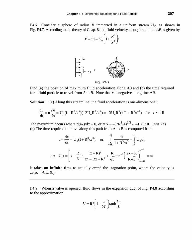
P4.7 Consider a sphere of radius R immersed in a uniform stream Uo, as shown in Fig. P4.7. According to the theory of Chap. 8, the fluid velocity along streamline AB is given by
3
o 3u 1
RU
x
V i i
Fig. P4.7
Find (a) the position of maximum fluid acceleration along AB and (b) the time required for a fluid particle to travel from A to B. Note that x is negative along line AB.
Solution: (a) Along this streamline, the fluid acceleration is one-dimensional:
3 3 3 4 3 4 3 7o o o
du uu U (1 R /x )( 3U R /x ) 3U R (x R x ) for x R
dt x
The maximum occurs where d(ax)/dx 0, or at x –(7R3/4)1/3 –1.205R Ans. (a) (b) The time required to move along this path from A to B is computed from
R t3 3
o o3 34R 0
dx dxu U (1 R /x ), or: U dt,
dt 1 R /x
R
4R
21
o 2 2
R (x R) R 2x Ror: U t x ln tan
6 x Rx R 3 R 3
It takes an infinite time to actually reach the stagnation point, where the velocity is zero. Ans. (b)
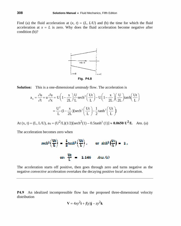
P4.8 When a valve is opened, fluid flows in the expansion duct of Fig. P4.8 according to the approximation
1 tanh2
x UtU
L L
V i
308 Solutions Manual Fluid Mechanics, Fifth Edition
Find (a) the fluid acceleration at (x, t) (L, L/U) and (b) the time for which the fluid acceleration at x L is zero. Why does the fluid acceleration become negative after condition (b)?
Fig. P4.8
Solution: This is a one-dimensional unsteady flow. The acceleration is
2x
u u x U Ut x U Uta u U 1 sech U 1 tanh
t x 2L L L 2L 2L L
2
2 2U x Ut 1 Ut(1 )[sech tanh ]
L 2L L 2 L
At (x, t) (L, L/U), ax (U2/L)(1/2)[sech2(1) – 0.5tanh2 (1)] 0.0650 U2/L Ans. (a) The acceleration becomes zero when
The acceleration starts off positive, then goes through zero and turns negative as the negative convective acceleration overtakes the decaying positive local acceleration.
P4.9 An idealized incompressible flow has the proposed three-dimensional velocity distribution
V 4xy2i f(y)j – zy2k
Chapter 4 Differential Relations for a Fluid Particle 309
Find the appropriate form of the function f(y) which satisfies the continuity relation.
Solution: Simply substitute the given velocity components into the incompressible continuity equation:
2 2 2 2(4 ) ( ) 4 0u v w f df
xy zy y yx y z x y z dy
2 2: 3 . Integrate: ( ) ( 3 )df
or y f y y dy Ans.dy
3y constant
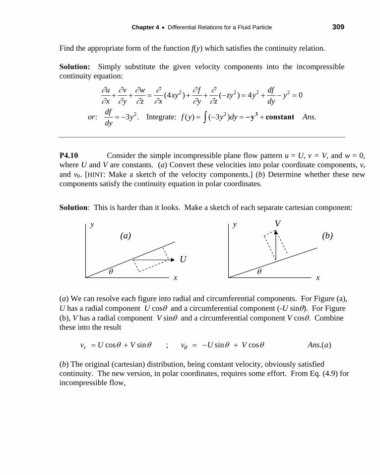
P4.10 Consider the simple incompressible plane flow pattern u = U, v = V, and w = 0, where U and V are constants. (a) Convert these velocities into polar coordinate components, vr
and v. [HINT: Make a sketch of the velocity components.] (b) Determine whether these new components satisfy the continuity equation in polar coordinates.
Solution: This is harder than it looks. Make a sketch of each separate cartesian component:
(a) We can resolve each figure into radial and circumferential components. For Figure (a), U has a radial component U cos and a circumferential component (-U sin). For Figure (b), V has a radial component V sin and a circumferential component V cos. Combine these into the result
cos sin ; sin cos .( )rv U V v U V Ans a
(b) The original (cartesian) distribution, being constant velocity, obviously satisfied continuity. The new version, in polar coordinates, requires some effort. From Eq. (4.9) for incompressible flow,
x
y
x
y
U
V (a) (b)
310 Solutions Manual Fluid Mechanics, Fifth Edition
1 1 1 1( ) ( ) [ ( cos sin )] ( sin cos )
1 1( cos sin ) ( cos sin ) Yes, satisfied. .( )
rr v v r U V U Vr r r r r r
U V U V Ans br r
0
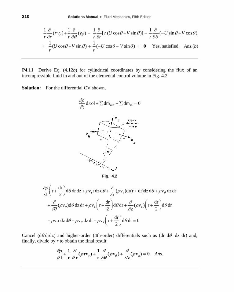
P4.11 Derive Eq. (4.12b) for cylindrical coordinates by considering the flux of an incompressible fluid in and out of the elemental control volume in Fig. 4.2.
Solution: For the differential CV shown,
out ind ol dm dm 0t
Fig. 4.2
r r
z z
r z
drr d dr dz v r dz d ( v )dr(r dr)dz d v dz dr
t 2 r
dr dr( v )d dz dr v r d dr ( v ) r d dr
2 z 2
drv r dz d v dz dr v r d dr 0
2
Cancel (d drdz) and higher-order (4th-order) differentials such as (dr d dz dr) and, finally, divide by r to obtain the final result:
.Ans r z
1 1rv v v 0
t r r r z
Chapter 4 Differential Relations for a Fluid Particle 311
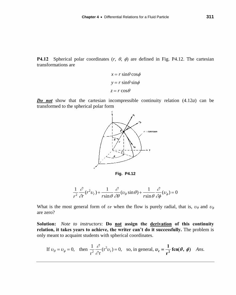
P4.12 Spherical polar coordinates (r, , ) are defined in Fig. P4.12. The cartesian transformations are
x r sin cos
y r sin sin
z r cos
Do not show that the cartesian incompressible continuity relation (4.12a) can be transformed to the spherical polar form
Fig. P4.12
22
1 1 1( ) ( sin ) ( ) 0
sin sinrrr r rr
What is the most general form of r when the flow is purely radial, that is, and are zero?
Solution: Note to instructors: Do not assign the derivation of this continuity relation, it takes years to achieve, the writer can’t do it successfully. The problem is only meant to acquaint students with spherical coordinates.
2r2
1If 0, then (r ) 0, so, in general,
rrAns.
r 2
1fcn ,
r
312 Solutions Manual Fluid Mechanics, Fifth Edition
P4.13 For an incompressible plane flow in polar coordinates, we are given
3 2cos sinrv r r
Find the appropriate form of circumferential velocity for which continuity is satisfied.
Solution: Substitute into continuity, Eq. (4.9), for incompressible flow:
3 2
2
3 2
1 1 1 1( ) ( ) [ ( cos sin )] ,
1or : 4 cos 3 sin
Integrate : 4 sin 3 cos ( ) .
rv
r v v r r rr r r r r r
vr r
r
v r r f r Ans
We can’t determine the form of the “constant of integration” f(r) without further information.
P4.14 For incompressible polar-coordinate flow, what is the most general form of a purely circulatory motion, (r, , t) and r 0, which satisfies continuity?
Solution: If vr 0, the plane polar coordinate continuity equation reduces to:
(1/r) ∂vθ/∂θ = 0 , or: vθ = fcn(r, t) Ans.
P4.15 What is the most general form of a purely radial polar-coordinate incompressible-flow pattern, r r(r, , t) and 0, which satisfies continuity?
Solution: If v 0, the plane polar coordinate continuity equation reduces to:
r1
(r ) 0, or: onlyr r
v Ans.
r1
fcnr
v
Chapter 4 Differential Relations for a Fluid Particle 313
________________________________________________________________________
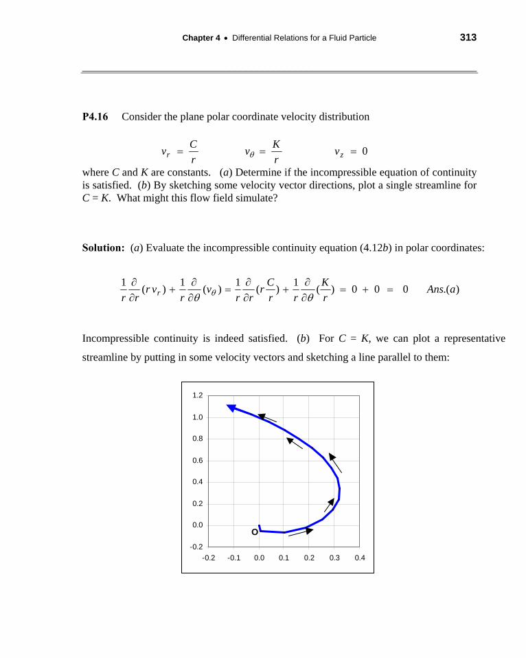
P4.16 Consider the plane polar coordinate velocity distribution
where C and K are constants. (a) Determine if the incompressible equation of continuity is satisfied. (b) By sketching some velocity vector directions, plot a single streamline for C = K. What might this flow field simulate?
Solution: (a) Evaluate the incompressible continuity equation (4.12b) in polar coordinates:
Incompressible continuity is indeed satisfied. (b) For C = K, we can plot a representative
streamline by putting in some velocity vectors and sketching a line parallel to them:
-0.2
0.0
0.2
0.4
0.6
0.8
1.0
1.2
-0.2 -0.1 0.0 0.1 0.2 0.3 0.4
O
0 zr vr
Kv
r
Cv
).(000)(1
)(1
)(1
)(1
aAnsr
K
rr
Cr
rrv
rvr
rr r
314 Solutions Manual Fluid Mechanics, Fifth Edition
The streamlines are logarithmic spirals moving out from the origin. [They have axisymmetry about O.] This simple distribution is often used to simulate a swirling flow such as a tornado.
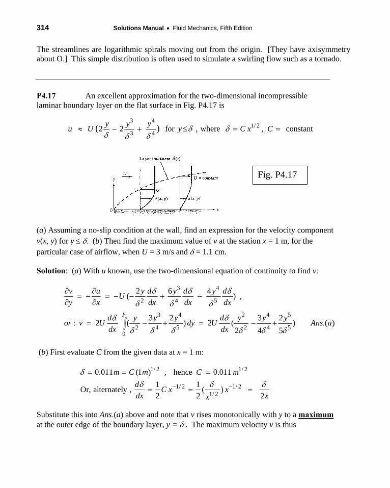
P4.17 An excellent approximation for the two-dimensional incompressible laminar boundary layer on the flat surface in Fig. P4.17 is
3 4
1/ 23 4
2 2 for , where , constant( )y y yu U y C x C
(a) Assuming a no-slip condition at the wall, find an expression for the velocity component v(x, y) for y . (b) Then find the maximum value of v at the station x = 1 m, for the particular case of airflow, when U = 3 m/s and = 1.1 cm.
Solution: (a) With u known, use the two-dimensional equation of continuity to find v:
3 4
2 4 5
3 4 2 4 5
2 4 5 2 4 50
2 6 4( ) ,
3 2 3 2: 2 ( ) 2 ( ) .( )
2 4 5
y
v u y d y d y dU
y x dx dx dx
d y y y d y y yor v U dy U Ans a
dx dx
(b) First evaluate C from the given data at x = 1 m:
1/ 2 1/ 2
1/ 2 1/ 21/ 2
0.011 (1 ) , hence 0.011
1 1Or, alternately , ( )
2 2 2
m C m C m
dC x x
dx xx
Substitute this into Ans.(a) above and note that v rises monotonically with y to a maximum at the outer edge of the boundary layer, y = . The maximum velocity v is thus
Fig. P4.17
Chapter 4 Differential Relations for a Fluid Particle 315
max1 3 2 0.011 3
2 ( ) 2(3 )[ ]( ) .( )2 4 5 2(1 ) 20
d m mv U Ans b
dx s m
m0.0050
s
This is slightly smaller than the exact value of vmax from laminar boundary theory (Chap. 7).
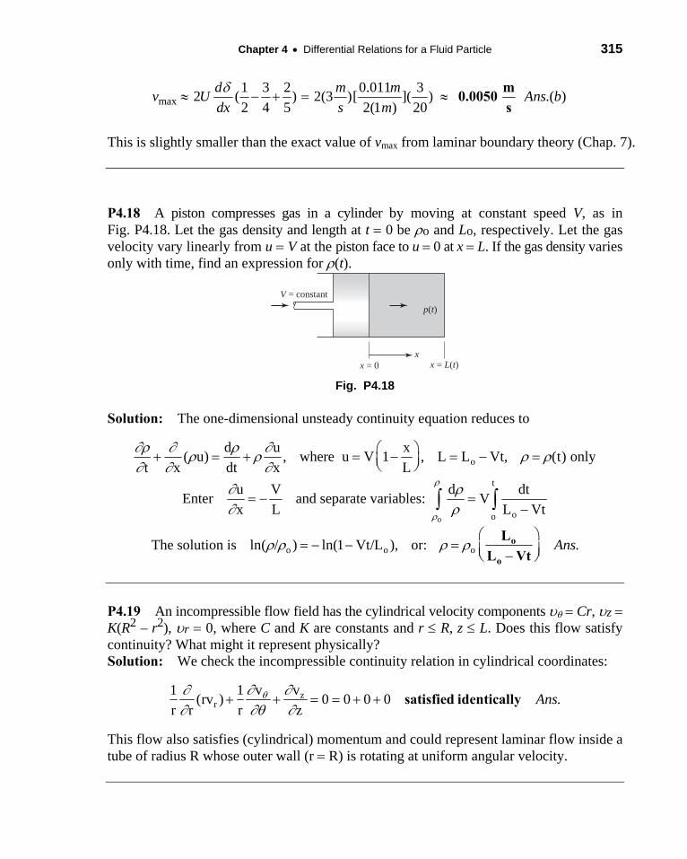
P4.18 A piston compresses gas in a cylinder by moving at constant speed V, as in Fig. P4.18. Let the gas density and length at t 0 be o and Lo, respectively. Let the gas velocity vary linearly from u V at the piston face to u 0 at x L. If the gas density varies only with time, find an expression for (t).
V = constant
x = 0 x = L(t)
p(t)
x
Fig. P4.18
Solution: The one-dimensional unsteady continuity equation reduces to
od u x
( u) , where u V 1 , L L Vt, (t) onlyt x dt x L
o
t
oo
u V d dtEnter and separate variables: V
x L L Vt
o o oThe solution is ln( / ) ln(1 Vt/L ), or: .Anso
o
L
L Vt
P4.19 An incompressible flow field has the cylindrical velocity components Cr, z K(R2 – r2), r 0, where C and K are constants and r R, z L. Does this flow satisfy continuity? What might it represent physically? Solution: We check the incompressible continuity relation in cylindrical coordinates:
zr
v1 1 v(rv ) 0 0 0 0 .
r r r zAns
satisfied identically
This flow also satisfies (cylindrical) momentum and could represent laminar flow inside a tube of radius R whose outer wall (r R) is rotating at uniform angular velocity.
316 Solutions Manual Fluid Mechanics, Fifth Edition
P4.20 A two-dimensional incompressible velocity field has u K(1 – e–ay), for x L and 0 y . What is the most general form of v(x, y) for which continuity is satisfied and v vo at y 0? What are the proper dimensions for constants K and a?
Solution: We can find the appropriate velocity v from two-dimensional continuity:
ayu[K(1 e )] 0, or: fcn(x) only
y x x
vv
oSince at y 0 for all x, then it must be that .v v Ans o const v v
The dimensions of K are {K} {L/T} and the dimensions of a are {L–1}. Ans.
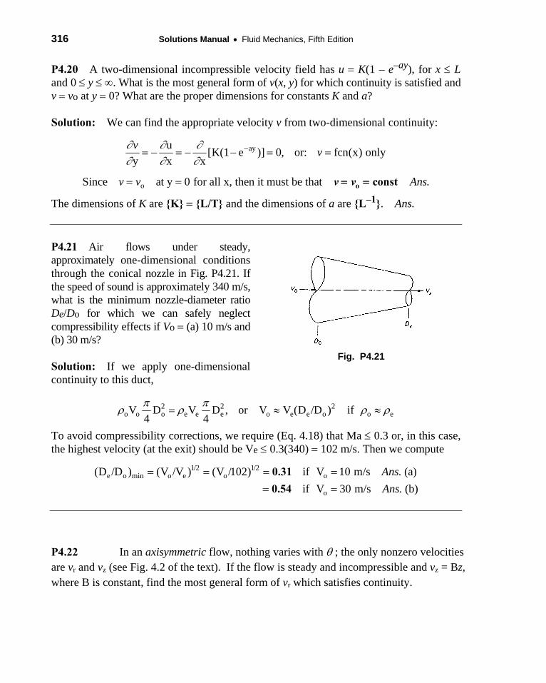
P4.21 Air flows under steady, approximately one-dimensional conditions through the conical nozzle in Fig. P4.21. If the speed of sound is approximately 340 m/s, what is the minimum nozzle-diameter ratio De/Do for which we can safely neglect compressibility effects if Vo (a) 10 m/s and (b) 30 m/s?
Solution: If we apply one-dimensional continuity to this duct,
Fig. P4.21
2 2 2o o o e e e o e e o o eV D V D , or V V (D /D ) if
4 4
To avoid compressibility corrections, we require (Eq. 4.18) that Ma 0.3 or, in this case, the highest velocity (at the exit) should be Ve 0.3(340) 102 m/s. Then we compute
1/2 1/2e o min o e o o(D /D ) (V /V ) (V /102) if V 10 m/s . (a)Ans 0.31
oif V 30 m/s . (b)Ans 0.54
P4.22 In an axisymmetric flow, nothing varies with ; the only nonzero velocities are vr and vz (see Fig. 4.2 of the text). If the flow is steady and incompressible and vz = Bz, where B is constant, find the most general form of vr which satisfies continuity.
Chapter 4 Differential Relations for a Fluid Particle 317
Solution: With no variation and no v, the equation of continuity (4.9) becomes
2
1 1( ) 0 ( ) ( ) ,
or : ( ) ; Integrate : ( )2
( )Finally, .
2
zr r
r r
r
vr v r v Bz
r r z r r zB
r v B r r v r f zr
B f zv r Ans
r
The “function of integration”, f(z), is arbitrary, at least until boundary conditions are set.
__________________________________________________________________________ P4.23 A tank volume V contains gas at conditions (o, po, To). At time t 0 it is punctured by a small hole of area A. According to the theory of Chap. 9, the mass flow out of such a hole is approximately proportional to A and to the tank pressure. If the tank temperature is assumed constant and the gas is ideal, find an expression for the variation of density within the tank.
Solution: This problem is a realistic approximation of the “blowdown” of a high-pressure tank, where the exit mass flow is choked and thus proportional to tank pressure. For a control volume enclosing the tank and cutting through the exit jet, the mass relation is
tank exit exitd d
(m ) m 0, or: ( ) m C p A, where C constantdt dt
o
p(t) to
o p o
CRT Ap dpIntroduce and separate variables: dt
RT p
The solution is an exponential decay of tank density: p po exp(–CRToAt/V ). Ans.
P4.24 For incompressible laminar flow between parallel plates (see Fig. 4.12b), the flow is two-dimensional (v 0) if the walls are porous. A special case solution is
2 2( ) ( )u A Bx h y , where A and B are constants. (a) Find a general formula for
velocity v if v = 0 at y = 0. (b) What is the value of the constant B if v = vw at y = +h? Solution: (a) Use the equation of continuity to find the velocity v:
318 Solutions Manual Fluid Mechanics, Fifth Edition
2 2
32 2 2
32
( )( )
Integrate : ( ) ( ) ( )3
If 0 0, then ( ) 0. ( ) .( )3
v uB h y
y x
yv B h y dy B h y f x
yv at y f x v B h y Ans a
(b) Just simply introduce this boundary condition into the answer to part (a):
3
33
3( ) ( ) , .( )
3 2w
wvh
v y h v B h hence B Ans bh
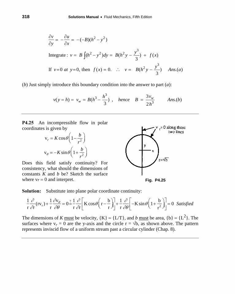
P4.25 An incompressible flow in polar coordinates is given by
2v cos 1r
bK
r
2v sin 1
bK
r
Does this field satisfy continuity? For consistency, what should the dimensions of constants K and b be? Sketch the surface where vr 0 and interpret.
Fig. P4.25
Solution: Substitute into plane polar coordinate continuity:
r 2
v1 1 1 b 1 b(rv ) 0 K cos r K sin 1 0
r r r r r r r rSatisfied
The dimensions of K must be velocity, {K} {L/T}, and b must be area, {b} {L2}. The surfaces where vr = 0 are the y-axis and the circle r = b, as shown above. The pattern represents inviscid flow of a uniform stream past a circular cylinder (Chap. 8).
Chapter 4 Differential Relations for a Fluid Particle 319
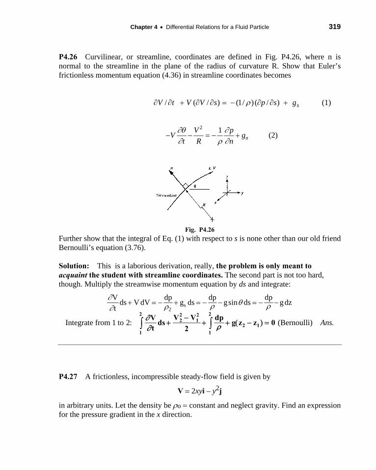
P4.26 Curvilinear, or streamline, coordinates are defined in Fig. P4.26, where n is normal to the streamline in the plane of the radius of curvature R. Show that Euler’s frictionless momentum equation (4.36) in streamline coordinates becomes / ( / ) (1/ ) ( / ) sV t V V s p s g (1)
2 1
nV p
V gt R n
(2)
Fig. P4.26
Further show that the integral of Eq. (1) with respect to s is none other than our old friend Bernoulli’s equation (3.76).
Solution: This is a laborious derivation, really, the problem is only meant to acquaint the student with streamline coordinates. The second part is not too hard, though. Multiply the streamwise momentum equation by ds and integrate:
s2
V dp dp dpds V dV g ds gsin ds g dz
t
Integrate from 1 to 2: (Bernoulli) .Ans
2 22 22 1
2 11 1
V V dpVds g z z 0
t 2
P4.27 A frictionless, incompressible steady-flow field is given by
V 2xyi – y2j
in arbitrary units. Let the density be o constant and neglect gravity. Find an expression for the pressure gradient in the x direction.
320 Solutions Manual Fluid Mechanics, Fifth Edition
Solution: For this (gravity-free) velocity, the momentum equation is
2ou v p, or: [(2xy)(2y ) ( y )(2x 2y )] p
x y
V Vi i j
2 3oSolve for p (2xy 2y ), or: .Ans 2
op
i j 2xyx
P4.28 Consider the incompressible flow field of Prob. P4.6, with velocity components u = 2y, v = 8x, w = 0. Neglect gravity and assume constant viscosity. (a) Determine whether this flow satisfies the Navier-Stokes equations. (b) If so, find the pressure distribution p(x, y) if the pressure at the origin is po.
Solution: In Prob. P4.6 we found the accelerations, so we can proceed to Navier-Stokes:
2
2
( ) [0 (8 )(2)] 0 0; 16
( ) [(2 )(8) 0] 0 0; 16
x
y
u u p p pu v x g u x
x y x x x
v v p p pu v y g v y
x y y y y
Noting that 2 /( ) 0 in both cases, we conclude .( )p x y Ans a Yes, satisfies Navier - Stokes.
(b) The pressure gradients are simple, so we may easily integrate:
2 2
2 2
, or : 16 16 8 ( )
If (0,0) , 8 ( ) .( )o o
p pdp dx dy p x dx y dy x y const
x y
p p then p p x y Ans b
This is an exact solution, but it is not Bernoulli’s equation. The flow is rotational.
P4.29 Consider a steady, two-dimensional, incompressible flow of a newtonian fluid with the velocity field u –2xy, v y2 – x2, and w 0. (a) Does this flow satisfy conservation of mass? (b) Find the pressure field p(x, y) if the pressure at point (x 0, y 0) is equal to pa.
Chapter 4 Differential Relations for a Fluid Particle 321
Solution: Evaluate and check the incompressible continuity equation:
( )0 2 2 0 0 au v w
y yx y z
Yes! Ans.
(b) Find the pressure gradients from the Navier-Stokes x- and y-relations: 2 2 2
2 2 2, :
u u u p u u uu v w or
x y z x x y z
2 2 2 3[ 2 ( 2 ) ( )( 2 )] (0 0 0), : 2 ( )p p
xy y y x x or xy xx x
and, similarly for the y-momentum relation, 2 2 2
2 2 2, :
v v v p v v vu v w or
x y z y x y z
2 2 2 3[ 2 ( 2 ) ( )(2 )] ( 2 2 0), : = 2 ( )p p
xy x y x y or x y yy y
The two gradients p/x and p/y may be integrated to find p(x, y):
2 2 4
2 ( ), :2 4y Const
p x y xp dx f y then differentiate
x
2 2 3 3 42 ( ) 2 ( ), 2 , : ( )2
p df dfx y x y y whence y or f y y C
y dy dy
2 2 4 4: (2 ) ( , ) (0,0), :2 aThus p x y x y C p at x y or
aC p
Finally, the pressure field for this flow is given by
(b)Ans. 2 2 4 4ap p (2x y x y )
P4.30 For the velocity distribution of Prob. P4.4, determine if (a) the equation of continuity
and (b) the Navier-Stokes equation are satisfied. (c) If the latter is true, find the pressure
distribution p(x,y) when the pressure at the origin equals po. Neglect gravity.
Solution: Recall that we were given u = Uo(1+x/L) and v = -Uo y/L. (a) Test continuity:
322 Solutions Manual Fluid Mechanics, Fifth Edition
(b) Now substitute these velocities into the x- and y- Navier-Stokes equations:
Solve for the two pressure gradients and cross-differentiate to see if they agree:
Thus, before finding p(x,y), we know this is an exact solution to Navier-Stokes. Ans.(b)
(c) Integrate the two pressure gradients to find the pressure distribution:
This is the same as Bernoulli’s equation, but that is a bit hard to see.
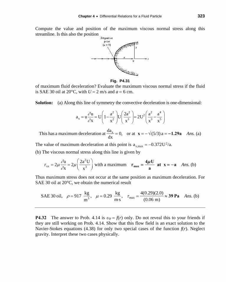
P4.31 According to potential theory (Chap. 8) for the flow approaching a rounded two-dimensional body, as in Fig. P4.31, the velocity approaching the stagnation point is given by u U(1 – a2/x2), where a is the nose radius and U is the velocity far upstream.
).(.satisfiedOK,0)()]1([ aAnsL
U
L
U
L
yU
yL
xU
xy
v
x
u oooo
011
))(()0()1(
011
)0)(()1(
2
2
y
pv
y
p
L
U
L
yU
L
xU
y
vv
x
vu
x
pu
x
p
L
yU
L
U
L
xU
y
uv
x
uu
ooo
oo
o
bothfor0Check)1(222
yx
p
L
y
L
U
y
p
L
x
L
U
x
p oo
).()22
(
2,Then;)()
2(
222
2222
cAnspL
y
L
xx
L
Up
constL
y
L
Uf
dy
df
y
pyf
L
xx
L
Udx
x
pp
oo
oo
Chapter 4 Differential Relations for a Fluid Particle 323
Compute the value and position of the maximum viscous normal stress along this streamline. Is this also the position
Fig. P4.31
of maximum fluid deceleration? Evaluate the maximum viscous normal stress if the fluid is SAE 30 oil at 20°C, with U 2 m/s and a 6 cm.
Solution: (a) Along this line of symmetry the convective deceleration is one-dimensional:
2 2 2 42
x 2 3 3 5
u a 2a a aa u U 1 U 2U
x x x x x
xdaThis has a maximum deceleration at 0, or at (5/3) a . (a)
dxAns x 1.29a
The value of maximum deceleration at this point is 2x,maxa 0.372U /a.
(b) The viscous normal stress along this line is given by
2
xx 3
u 2a U2 2 with a maximum . (b)
x xAns
max
4 Uat x a
a
Thus maximum stress does not occur at the same position as maximum deceleration. For SAE 30 oil at 20°C, we obtain the numerical result
max3
kg kg 4(0.29)(2.0)SAE 30 oil, 917 , 0.29 , . (b)
m s (0.06 m)mAns
39 Pa
P4.32 The answer to Prob. 4.14 is f(r) only. Do not reveal this to your friends if they are still working on Prob. 4.14. Show that this flow field is an exact solution to the Navier-Stokes equations (4.38) for only two special cases of the function f(r). Neglect gravity. Interpret these two cases physically.
324 Solutions Manual Fluid Mechanics, Fifth Edition
Solution: Given v f(r) and vr vz 0, we need only satisfy the -momentum relation:
2
r 2 2 2
v v v v v v1 p 1 1v r ,
r r r r r r r r
2
1 d df for: (0 0) 0 r 0 , or:
r dr dr r 2
1 1f f f 0
r r
This is the ‘equidimensional’ ODE and always has a solution in the form of a power-law, f Crn. The two relevant solutions for these particular coefficients are n = 1:
f1 C1r (solid-body rotation); f2 C2/r (irrotational vortex) Ans.
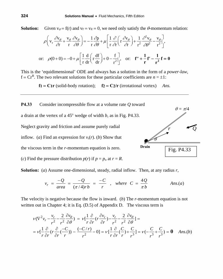
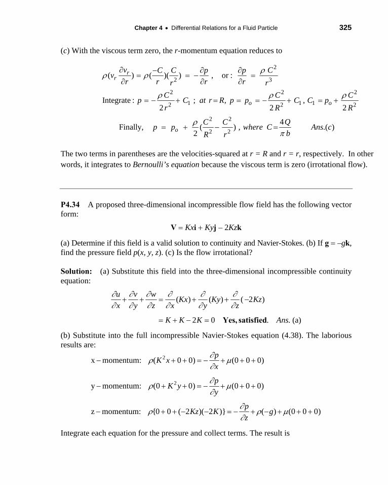
P4.33 Consider incompressible flow at a volume rate Q toward
a drain at the vertex of a 45 wedge of width b, as in Fig. P4.33.
Neglect gravity and friction and assume purely radial
inflow. (a) Find an expression for vr(r). (b) Show that
the viscous term in the r-momentum equation is zero.
(c) Find the pressure distribution p(r) if p = po at r = R.
Solution: (a) Assume one-dimensional, steady, radial inflow. Then, at any radius r,
4
, .( )( / 4)r
Q Q C Qv where C Ans a
area r b r b
The velocity is negative because the flow is inward. (b) The r-momentum equation is not written out in Chapter 4; it is Eq. (D.5) of Appendix D. The viscous term is
22 2 2 2
2 3 3 3
2 1 2( ) [ ( ) ]
1 ( / ) 1[ ( ( )) 0] [ ( ) ] ( ) .( )
r r rr
v vv v vv r
r r rr r r rC C r C C C C
r Ans br r r r r r rr r r r
0
r
Q
= /4
Drain Fig. P4.33
Chapter 4 Differential Relations for a Fluid Particle 325
(c) With the viscous term zero, the r-momentum equation reduces to
2
2 3
2 2 2
1 1 12 2 2
2 2
2 2
( ) ( )( ) , or :
Integrate : ; , ,2 2 2
4Finally, ( ) , .( )
2
rr
o o
o
v CC C p pv
r r r rr r
C C Cp C at r R p p C C p
r R R
QC Cp p where C Ans c
bR r
The two terms in parentheses are the velocities-squared at r = R and r = r, respectively. In other words, it integrates to Bernoulli’s equation because the viscous term is zero (irrotational flow).
P4.34 A proposed three-dimensional incompressible flow field has the following vector form:
V Kxi Kyj – 2Kzk
(a) Determine if this field is a valid solution to continuity and Navier-Stokes. (b) If g –gk, find the pressure field p(x, y, z). (c) Is the flow irrotational?
Solution: (a) Substitute this field into the three-dimensional incompressible continuity equation:
.
( ) ( ) ( 2 )
2 0 (a)
u v wKx Ky Kz
x y z x y z
K K K Ans.
Yes, satisfied
(b) Substitute into the full incompressible Navier-Stokes equation (4.38). The laborious results are:
2x momentum: ( 0 0) (0 0 0)p
K xx
2y momentum: (0 0) (0 0 0)p
K yy
z momentum: {0 0 ( 2 )( 2 )} ( ) (0 0 0)p
Kz K gz
Integrate each equation for the pressure and collect terms. The result is
326 Solutions Manual Fluid Mechanics, Fifth Edition
p p(0,0,0) – gz – (/2)K2(x2 y2 4z2) Ans. (b)
Note that the last term is identical to (/2)(u2 v2 w2), in other words, Bernoulli’s equation. (c) For irrotational flow, the curl of the velocity field must be zero:
V i(0 – 0) j(0 – 0) k(0 – 0) 0 Yes, irrotational. Ans. (c)
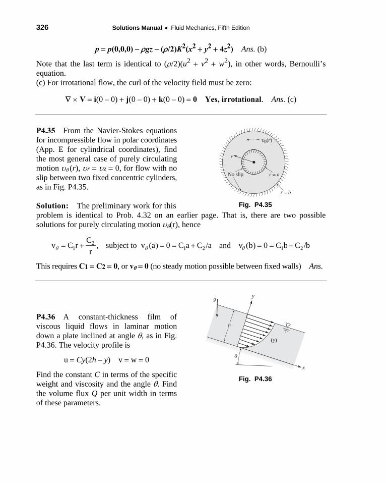
P4.35 From the Navier-Stokes equations for incompressible flow in polar coordinates (App. E for cylindrical coordinates), find the most general case of purely circulating motion (r), r z 0, for flow with no slip between two fixed concentric cylinders, as in Fig. P4.35.
Solution: The preliminary work for this
r
No slip
r = b
r = a
υ (r)θ
Fig. P4.35
problem is identical to Prob. 4.32 on an earlier page. That is, there are two possible solutions for purely circulating motion (r), hence
21 1 2 1 2
Cv C r , subject to v (a) 0 C a C /a and v (b) 0 C b C /b
r
This requires C1 C2 0, or v 0 (no steady motion possible between fixed walls) Ans.
P4.36 A constant-thickness film of viscous liquid flows in laminar motion down a plate inclined at angle , as in Fig. P4.36. The velocity profile is
u Cy(2h – y) v w 0
Find the constant C in terms of the specific weight and viscosity and the angle . Find the volume flux Q per unit width in terms of these parameters.
(y)
g y
x
h
θ
Fig. P4.36
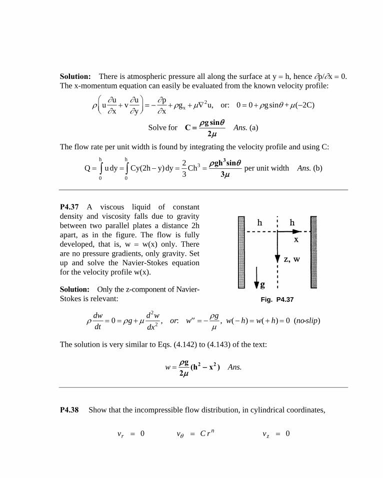
Solution: There is atmospheric pressure all along the surface at y h, hence p/x 0. The x-momentum equation can easily be evaluated from the known velocity profile:
2x
u u pu v g u, or: 0 0 gsin + ( 2C)
x y x
Solve for . (a)Ansg sin
C2
The flow rate per unit width is found by integrating the velocity profile and using C:
h h3
0 0
2Q udy Cy(2h y)dy Ch per unit width . (b)
3Ans
3gh sin
3
P4.37 A viscous liquid of constant density and viscosity falls due to gravity between two parallel plates a distance 2h apart, as in the figure. The flow is fully developed, that is, w w(x) only. There are no pressure gradients, only gravity. Set up and solve the Navier-Stokes equation for the velocity profile w(x).
Solution: Only the z-component of Navier-Stokes is relevant:
Fig. P4.37
2
20 , : , ( ) ( ) 0 ( )
dw d w gg or w w h w h no-slip
dt dx
The solution is very similar to Eqs. (4.142) to (4.143) of the text:
.w Ans
2 2g(h x )
2
P4.38 Show that the incompressible flow distribution, in cylindrical coordinates,
00 zn
r vrCvv
328 Solutions Manual Fluid Mechanics, Fifth Edition
where C is a constant, (a) satisfies the Navier-Stokes equation for only two values of n. Neglect gravity. (b) Knowing that p = p(r) only, find the pressure distribution for each case, assuming that the pressure at r = R is po. What might these two cases represent?
Solution: (a) The important direction here is the -momentum equation, Eq. (D.6):
Cancel C and and rn-2. These terms equal zero only if n2 = 1, or n = 1. Ans.(a).
(b) Find the respective pressure distributions for n = 1 and n = -1. Use Eq. (D.5), which
reduces simply to p/r = v2/r. Try this for each distribution, n = 1:
Case 1, v = Cr, is solid-body rotation. Case 2, v = C/r, is an irrotational potential vortex.
0)(])(1
[
:or,]))((1
[)0(0000
:or,)2
(1
r
1 )(
22221
222
222
nnnn
nn
r
CrrCnCrrnCrrr
r
CrCr
rr
rrr
vv
v
rr
vv
p
rvvv
t
v
V
).()11
(2
:or;)/(
:1,2
).()(2
:or;)(
:1,1
222
222
122
222
bAnsrR
Cppdr
r
rCdpnCase
bAnsRrC
ppdrr
rCdpnCase
or
R
p
p
or
R
p
p
o
o
Chapter 4 Differential Relations for a Fluid Particle 329
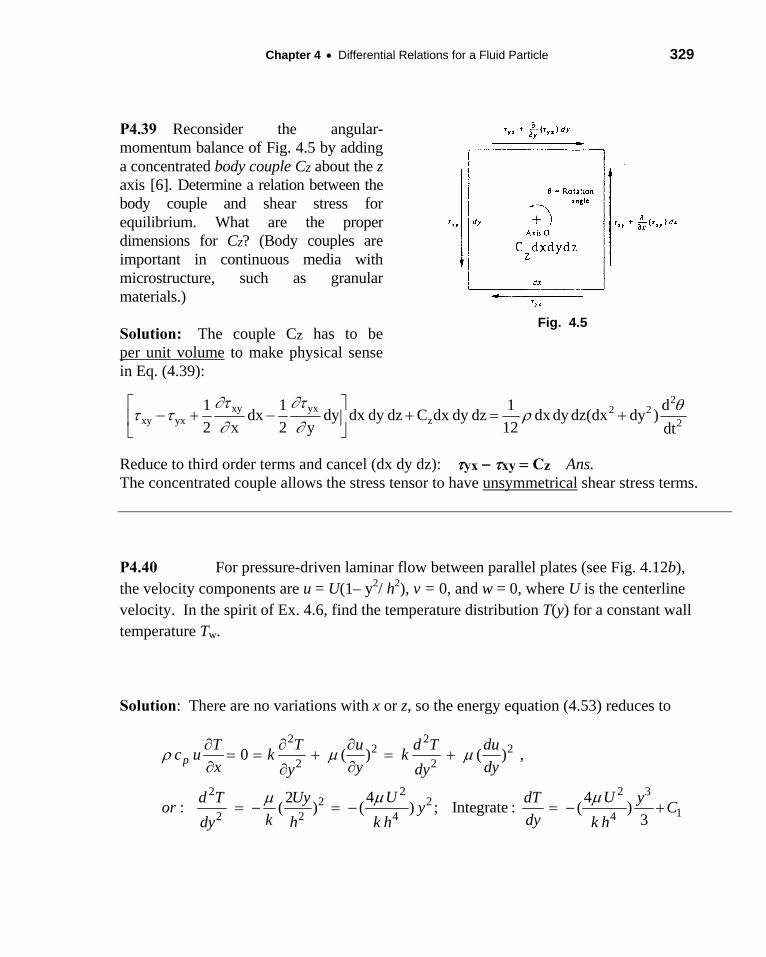
P4.39 Reconsider the angular-momentum balance of Fig. 4.5 by adding a concentrated body couple Cz about the z axis [6]. Determine a relation between the body couple and shear stress for equilibrium. What are the proper dimensions for Cz? (Body couples are important in continuous media with microstructure, such as granular materials.)
Solution: The couple Cz has to be per unit volume to make physical sense in Eq. (4.39):
Fig. 4.5
2xy yx 2 2
xy yx z 2
1 1 1 ddx dy dx dy dz C dx dy dz dx dy dz(dx dy )
2 x 2 y 12 dt
Reduce to third order terms and cancel (dx dy dz): yx xy Cz Ans. The concentrated couple allows the stress tensor to have unsymmetrical shear stress terms.
P4.40 For pressure-driven laminar flow between parallel plates (see Fig. 4.12b), the velocity components are u = U(1– y2/ h2), v = 0, and w = 0, where U is the centerline velocity. In the spirit of Ex. 4.6, find the temperature distribution T(y) for a constant wall temperature Tw.
Solution: There are no variations with x or z, so the energy equation (4.53) reduces to
2 22 2
2 2
2 22 32 2
12 2 4 4
0 ( ) ( ) ,
4 42: ( ) ( ) ; Integrate : ( )
3
pT T u d T du
c u k kx y dyy dy
U Ud T Uy dT yor y C
k dydy h k h k h
330 Solutions Manual Fluid Mechanics, Fifth Edition
The condition T = Tw at h is equivalent to dT/dy = 0 at y = 0. Thus C1 = 0. Integrate again:
2 2 24 4
2 2 24 4
4 4( ) ; at : ( ) ,
12 12 3
w w
U U Uy hT C y h T T C C T
kk h k h
The final solution for T(y) is, like Ex. 4.6, a quartic polynomial:
2 4
4( ) (1 ) .
3wU y
T y T Ansk h
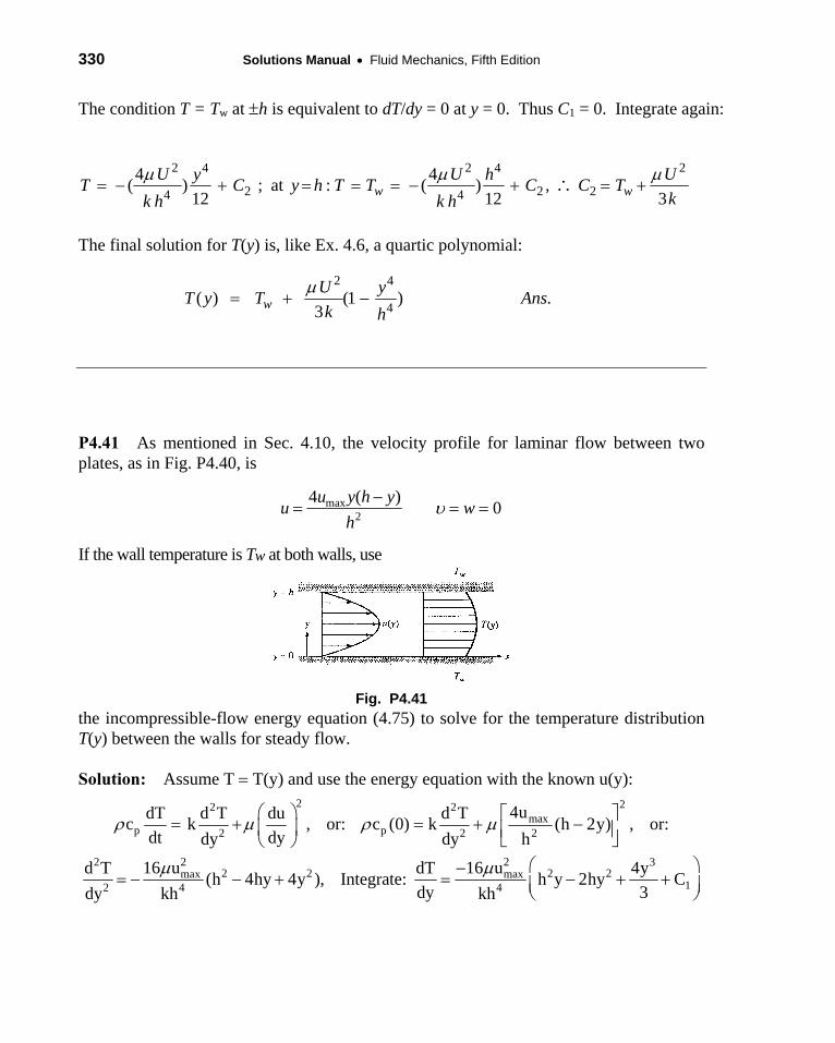
P4.41 As mentioned in Sec. 4.10, the velocity profile for laminar flow between two plates, as in Fig. P4.40, is
max2
4 ( )0
u y h yu w
h
If the wall temperature is Tw at both walls, use
Fig. P4.41
the incompressible-flow energy equation (4.75) to solve for the temperature distribution T(y) between the walls for steady flow.
Solution: Assume T T(y) and use the energy equation with the known u(y): 2 22 2
maxp p2 2 2
4udT d T du d Tc k , or: c (0) k (h 2y) , or:
dt dydy dy h
2 22 32 2 2 2max max
12 4 4
16 u 16 ud T dT 4y(h 4hy 4y ), Integrate: h y 2hy C
dy 3dy kh kh
Chapter 4 Differential Relations for a Fluid Particle 331
Before integrating again, note that dT/dy 0 at y h/2 (the symmetry condition), so C1 –h3/6. Now integrate once more:
2 2 3 42max
1 24
16 u y y yT h 2h C y C
2 3 3kh
If T Tw at y 0 and at y h, then C2 Tw. The final solution is:
.Ans
2 2 3 4max
w 2 3 4
8 u y y 4y 2yT T
k 3h h 3h 3h
This is exactly the same solution as Problem P4.40 above, except that, here, the coordinate y is measured from the boo tom wall rather than the centerline.
P4.42 Suppose that we wish to analyze the rotating, partly-full cylinder of Fig. 2.23 as a spin-up problem, starting from rest and continuing until solid-body-rotation is achieved. What are the appropriate boundary and initial conditions for this problem?
Solution: Let V V(r, z, t). The initial condition is: V(r, z, 0) 0. The boundary conditions are
Along the side walls: v(R, z, t) R, vr(R, z, t) 0, vz(R, z, t) 0.
At the bottom, z 0: v(r, 0, t) r, vr(r, 0, t) 0, vz(r, 0, t) 0.
At the free surface, z : p patm, rz z 0.
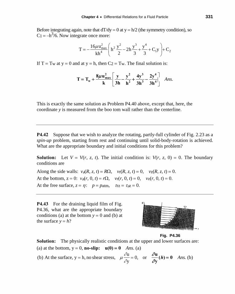
P4.43 For the draining liquid film of Fig. P4.36, what are the appropriate boundary conditions (a) at the bottom y 0 and (b) at the surface y h?
Fig. P4.36
Solution: The physically realistic conditions at the upper and lower surfaces are:
(a) at the bottom, y 0, no-slip: u(0) 0 Ans. (a) u
(b) At the surface, y h, no shear stress, 0, or . (b)y
Ans
u
( ) 0y
h
332 Solutions Manual Fluid Mechanics, Fifth Edition
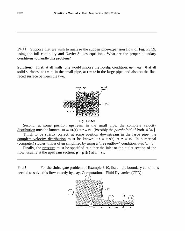
P4.44 Suppose that we wish to analyze the sudden pipe-expansion flow of Fig. P3.59, using the full continuity and Navier-Stokes equations. What are the proper boundary conditions to handle this problem?
Solution: First, at all walls, one would impose the no-slip condition: ur uz 0 at all solid surfaces: at r r1 in the small pipe, at r r2 in the large pipe, and also on the flat-faced surface between the two.
Fig. P3.59
Second, at some position upstream in the small pipe, the complete velocity distribution must be known: u1 u1(r) at z z1. [Possibly the paraboloid of Prob. 4.34.]
Third, to be strictly correct, at some position downstream in the large pipe, the complete velocity distribution must be known: u2 u2(r) at z z2. In numerical (computer) studies, this is often simplified by using a “free outflow” condition, u/ z 0.
Finally, the pressure must be specified at either the inlet or the outlet section of the flow, usually at the upstream section: p p1(r) at z z1.
P4.45 For the sluice gate problem of Example 3.10, list all the boundary conditions needed to solve this flow exactly by, say, Computational Fluid Dynamics (CFD).
1
2
3
3
2
4
Chapter 4 Differential Relations for a Fluid Particle 333
Solution: There are four different kinds of boundary conditions needed, as labeled.
(1) Known velocity V1 upstream, and of course the depth y1 must be known.
(2) Known pressure patm at both the upstream and downstream free surfaces.
(3) No-slip (V = 0) all along the bottom and on the gate inner wall.
(4) The downstream flow is complicated because we don’t know V2 or y2 and therefore cannot specify them. What CFD modelers do is to have an adjustable upper boundary and specify that the exit flow is “smooth”, or “zero gradient”, that is, V/x = 0.
P4.46 Fluid from a large reservoir at temperature To flows into a circular pipe of radius R. The pipe walls are wound with an electric-resistance coil which delivers heat to the fluid at a rate qw (energy per unit wall area). If we wish to analyze this problem by using the full continuity, Navier-Stokes, and energy equations, what are the proper boundary conditions for the analysis?
Solution: Letting z 0 be the pipe entrance, we can state inlet conditions: typically uz(r, 0) U (a uniform inlet profile), ur(r, 0) 0, and T(r, 0) To, also uniform.
At the wall, r R, the no-slip and known-heat-flux conditions hold: uz(R, z) ur(R, z) 0 and k( T/ r) qw at (R, z) (assuming that qw is positive for heat flow in).
At the exit, z L, we would probably assume ‘free outflow’: uz/ z T/ z 0. Finally, we would need to know the pressure at one point, probably the inlet, z 0.
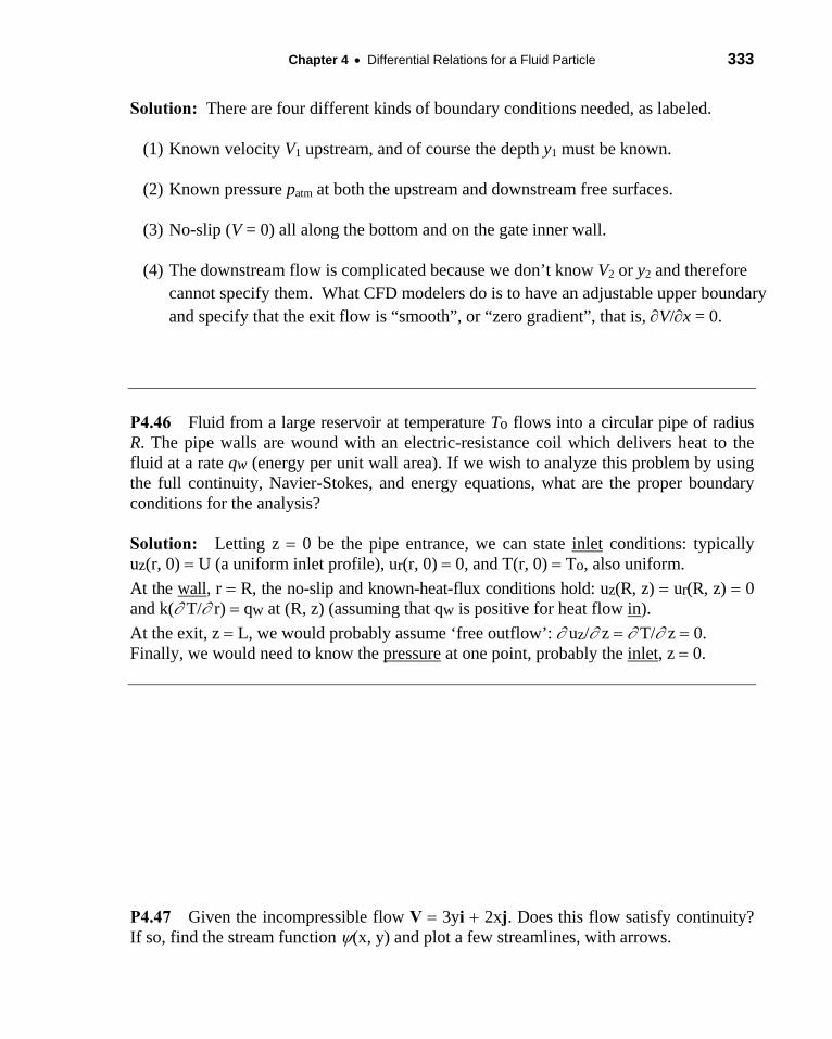
P4.47 Given the incompressible flow V 3yi 2xj. Does this flow satisfy continuity? If so, find the stream function (x, y) and plot a few streamlines, with arrows.
334 Solutions Manual Fluid Mechanics, Fifth Edition
Solution: With u 3y and v 2x, we may check u/ x v/ y 0 0 0, OK. Find the streamlines from u / y 3y and v –/x 2x. Integrate to find
.Ans 2 23
2y x
Set 0, 1, 2, etc. and plot some streamlines at right: flow around corners of half-angles 39 and 51.
39°51°
x
y
Fig. P4.47
P4.48 Consider the following two-dimensional incompressible flow, which clearly satisfies continuity:
u Uo constant, v Vo constant
Find the stream function (r, ) of this flow, that is, using polar coordinates.
Solution: In cartesian coordinates the stream function is quite easy:
u / y Uo and v –/x Vo or: Uoy – Vox constant
But, in polar coordinates, y rsin and x rcos. Therefore the desired result is
(r, ) Uor sin – Vor cos constant Ans.
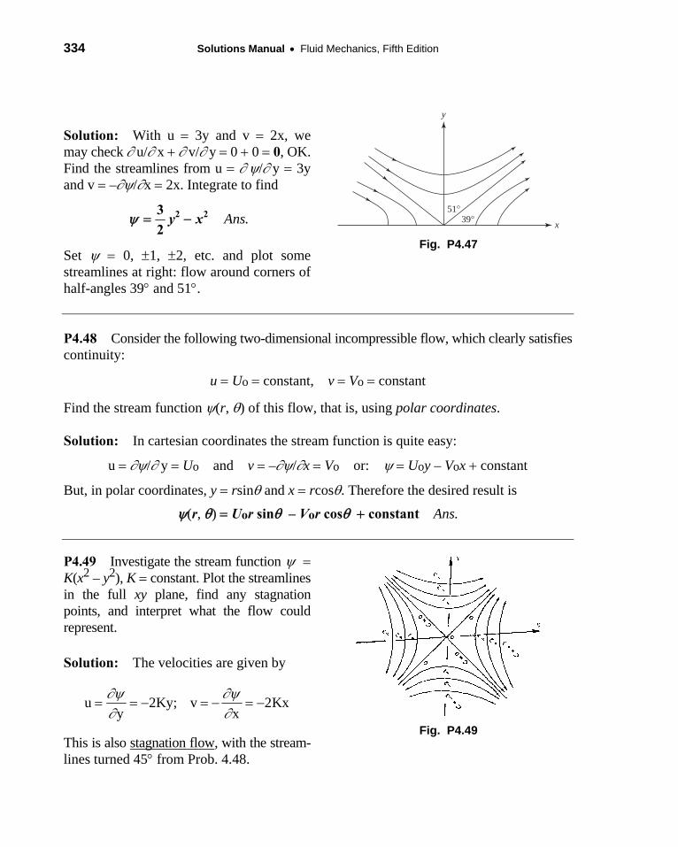
P4.49 Investigate the stream function K(x2 – y2), K constant. Plot the streamlines in the full xy plane, find any stagnation points, and interpret what the flow could represent.
Solution: The velocities are given by
u 2Ky; v 2Kxy x
This is also stagnation flow, with the stream-lines turned 45 from Prob. 4.48.
Fig. P4.49
P4.50 In 1851, George Stokes (of Navier-Stokes fame) solved the problem of steady incompressible low-Reynolds-number flow past a sphere, using spherical polar coordinates (r, ) – [Ref. 5, page 168]. In these coordinates, the equation of continuity is
2( sin ) ( sin ) 0rr v r vr
(a) Does a stream function exist for these coordinates? (b) If so, find its form.
Solution: Two velocity components and two continuity terms. Yes, exists! Ans.(a) (b) The stream function should be defined such that continuity takes the form
2 2
2
0 , or :
1 1; .( )
sin sinr
r r
v v Ans br r r
P4.51 The velocity profile for incompressible pressure-driven laminar flow between parallel plates (see Fig. 4.12b) has the form u = C(h2 – y2), where C is a constant. (a) Determine if a stream function exists. (b) If so, determine a formula for the stream function, Solution: (a) A stream function exists, for a single velocity component u, if u/x = 0, which it certainly is, since u is a function only of y. Yes, exists. Ans.(a) (b) Finding the stream function is just a matter of direct integration:
32 2 2
0 , hence is a function only of
( ) ; Integrate : ( ) .( )3
v yx
yu C h y C h y constant Ans b
y
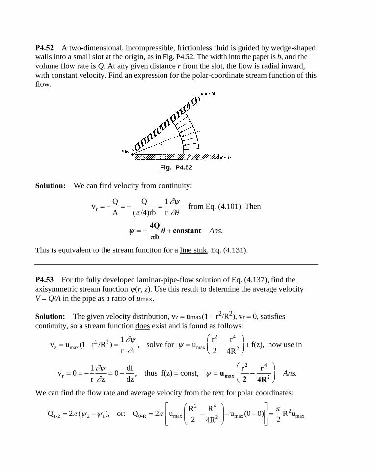
P4.52 A two-dimensional, incompressible, frictionless fluid is guided by wedge-shaped walls into a small slot at the origin, as in Fig. P4.52. The width into the paper is b, and the volume flow rate is Q. At any given distance r from the slot, the flow is radial inward, with constant velocity. Find an expression for the polar-coordinate stream function of this flow.
Fig. P4.52
Solution: We can find velocity from continuity:
rQ Q 1
v from Eq. (4.101). ThenA ( /4)rb r
.Ans 4Q constant
bθ
π
This is equivalent to the stream function for a line sink, Eq. (4.131).
P4.53 For the fully developed laminar-pipe-flow solution of Eq. (4.137), find the axisymmetric stream function (r, z). Use this result to determine the average velocity V Q/A in the pipe as a ratio of umax.
Solution: The given velocity distribution, vz umax(1 – r2/R2), vr 0, satisfies continuity, so a stream function does exist and is found as follows:
2 42 2
z max max 2
1 r rv u (1 r /R ) , solve for u f(z), now use in
r r 2 4R
r1 df
v 0 0 , thus f(z) const, .r z dz
Ans
2 4
max 2
r ru
2 4R
We can find the flow rate and average velocity from the text for polar coordinates:
2 42
1-2 2 1 0-R max max max2
R RQ 2 ( ), or: Q 2 u u (0 0) R u
2 24R
Chapter 4 Differential Relations for a Fluid Particle 337
2 2avg pipe maxThen V Q/A [( /2)R u /( R )] .Ans max
1u
2
338 Solutions Manual Fluid Mechanics, Fifth Edition
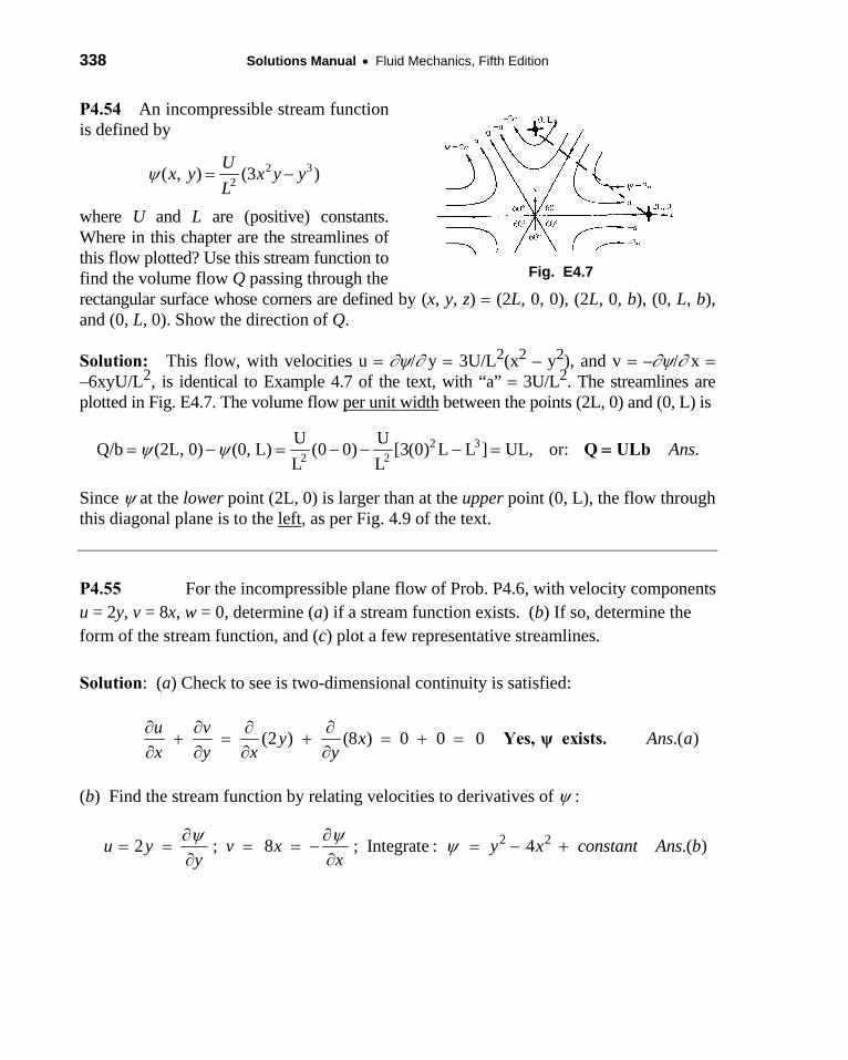
P4.54 An incompressible stream function is defined by
2 32
( , ) (3 )U
x y x y yL
where U and L are (positive) constants. Where in this chapter are the streamlines of this flow plotted? Use this stream function to find the volume flow Q passing through the
Fig. E4.7
rectangular surface whose corners are defined by (x, y, z) (2L, 0, 0), (2L, 0, b), (0, L, b), and (0, L, 0). Show the direction of Q.
Solution: This flow, with velocities u / y 3U/L2(x2 – y2), and v –/ x –6xyU/L2, is identical to Example 4.7 of the text, with “a” 3U/L2. The streamlines are plotted in Fig. E4.7. The volume flow per unit width between the points (2L, 0) and (0, L) is
2 32 2
U UQ/b (2L, 0) (0, L) (0 0) [3(0) L L ] UL, or: .
L LAns Q ULb
Since at the lower point (2L, 0) is larger than at the upper point (0, L), the flow through this diagonal plane is to the left, as per Fig. 4.9 of the text.
P4.55 For the incompressible plane flow of Prob. P4.6, with velocity components u = 2y, v = 8x, w = 0, determine (a) if a stream function exists. (b) If so, determine the form of the stream function, and (c) plot a few representative streamlines. Solution: (a) Check to see is two-dimensional continuity is satisfied:
(2 ) (8 ) 0 0 0 .( )u v
y x Ans ax y x y
Yes, ψ exists.
(b) Find the stream function by relating velocities to derivatives of :
2 22 ; 8 ; Integrate : 4 .( )u y v x y x constant Ans by x
Chapter 4 Differential Relations for a Fluid Particle 339
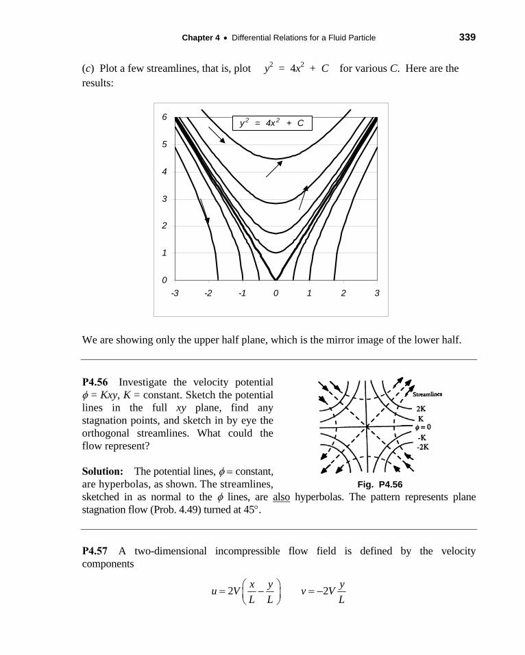
(c) Plot a few streamlines, that is, plot y2 = 4x2 + C for various C. Here are the results:
0
1
2
3
4
5
6
-3 -2 -1 0 1 2 3
y2 = 4x2 + C
We are showing only the upper half plane, which is the mirror image of the lower half.
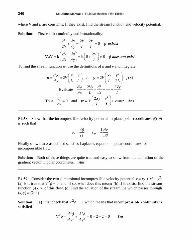
P4.56 Investigate the velocity potential = Kxy, K = constant. Sketch the potential lines in the full xy plane, find any stagnation points, and sketch in by eye the orthogonal streamlines. What could the flow represent?
Solution: The potential lines, constant, are hyperbolas, as shown. The streamlines,
Fig. P4.56
sketched in as normal to the lines, are also hyperbolas. The pattern represents plane stagnation flow (Prob. 4.49) turned at 45.
P4.57 A two-dimensional incompressible flow field is defined by the velocity components
2 2x y y
u V v VL L L
340 Solutions Manual Fluid Mechanics, Fifth Edition
where V and L are constants. If they exist, find the stream function and velocity potential.
Solution: First check continuity and irrotationality:
2 20
20 0
u v V V
x y L L
v u Vx
x y L
exists
does not exist
;
V k k
To find the stream function , use the definitions of u and v and integrate:
2
2 , 2 ( )2
x y xy yu V V f x
y L L L L
2 2Evaluate
Thus 0 and .
Vy df Vyv
x L dx L
dfAns
dx
xy y
V constL L
22
P4.58 Show that the incompressible velocity potential in plane polar coordinates (r,) is such that
1r r r
Finally show that as defined satisfies Laplace’s equation in polar coordinates for incompressible flow.
Solution: Both of these things are quite true and easy to show from the definition of the gradient vector in polar coordinates. Ans.
P4.59 Consider the two-dimensional incompressible velocity potential xy x2 – y2. (a) Is it true that 2 0, and, if so, what does this mean? (b) If it exists, find the stream function (x, y) of this flow. (c) Find the equation of the streamline which passes through (x, y) (2, 1).
Solution: (a) First check that 2 0, which means that incompressible continuity is satisfied.
2 22
2 20 2 2 0
x y
Yes
Chapter 4 Differential Relations for a Fluid Particle 341
(b) Now use to find u and v and then integrate to find .
2
2 , hence 2 ( )2
yu y x xy f x
x y
2
2 2 , hence ( )2
df xv x y y f x const
y x dx
The final stream function is thus . (b)Ans 2 212
2y x xy const
(c) The streamline which passes through (x, y) (2, 1) is found by setting a constant:
2 21 3 5( , ) (2, 1), (1 2 ) 2(2)(1) 4
2 2 2At x y
Thus the proper streamline is . (c)Ans 2 21 52
2 2y x xy
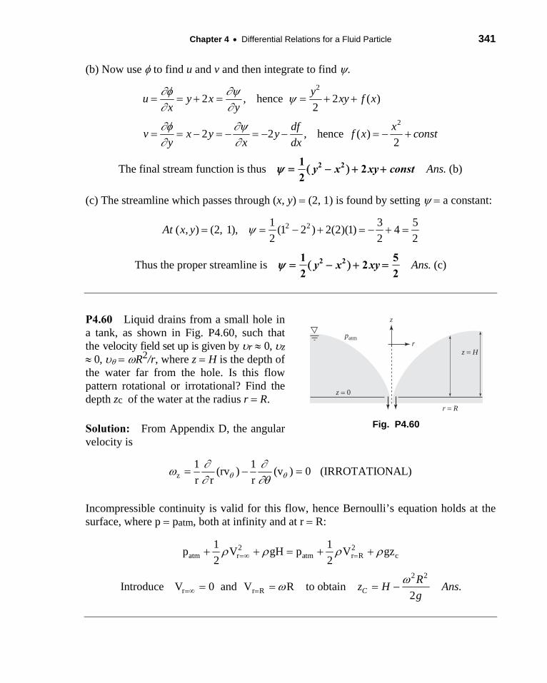
P4.60 Liquid drains from a small hole in a tank, as shown in Fig. P4.60, such that the velocity field set up is given by r 0, z 0, R2/r, where z H is the depth of the water far from the hole. Is this flow pattern rotational or irrotational? Find the depth zc of the water at the radius r R.
Solution: From Appendix D, the angular velocity is
patm
z
r
z = 0
r = R
z = H
Fig. P4.60
z1 1
(rv ) (v ) 0 (IRROTATIONAL)r r r
Incompressible continuity is valid for this flow, hence Bernoulli’s equation holds at the surface, where p patm, both at infinity and at r R:
2 2atm r atm r R c
1 1p V gH p V gz
2 2
2 2
r r RIntroduce V 0 and V R to obtain .2C
Rz H Ans
g
342 Solutions Manual Fluid Mechanics, Fifth Edition
P4.61 For the incompressible plane flow of Prob. P4.6, with velocity components u = 2y, v = 8x, w = 0, determine (a) if a velocity potential exists. (b) If so, determine the form of the velocity potential, and (c) plot a few representative potential lines. Solution: (a) A velocity potential exists if the vorticity is zero. Here, for plane flow in (x, y) coordinates, we need only evaluate rotation around the z axis:
2 8 2 6 0 Rotational , does not exist. .( )z zv u
Ans ax y
(b, c) There is no velocity potential – no plot, no formula. The flow has constant vorticity.
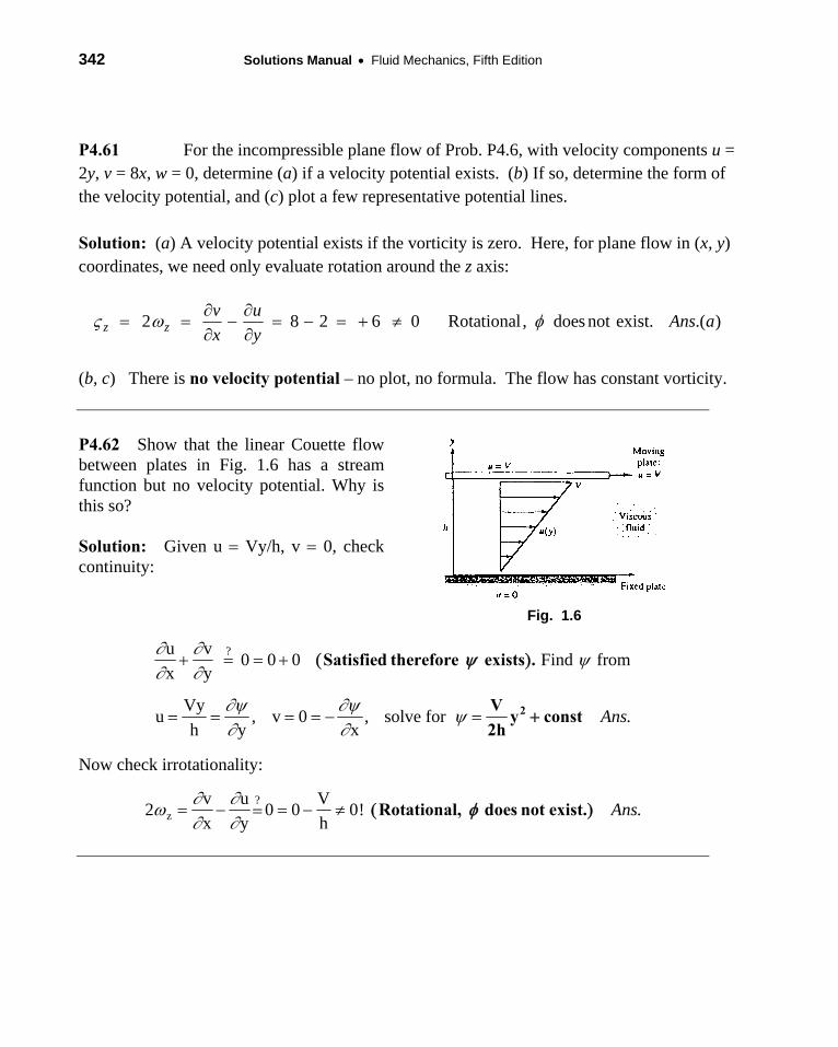
P4.62 Show that the linear Couette flow between plates in Fig. 1.6 has a stream function but no velocity potential. Why is this so?
Solution: Given u Vy/h, v 0, check continuity:
Fig. 1.6
?u v 0 0 0 Find from
x y
Satisfied therefore exists .
Vyu , v 0 , solve for .
h y xAns
2V
y const2h
Now check irrotationality:
?z
v u V2 0 0 0! .
x y hAns
Rotational, does not exist.
Chapter 4 Differential Relations for a Fluid Particle 343
P4.63 Find the two-dimensional velocity potential (r,) for the polar-coordinate flow pattern r Q/r, K/r, where Q and K are constants.
Solution: Relate these velocity components to the polar-coordinate definition of :
r Q K 1
v , v ; solve for .r r r r
Ans
Q ln(r) K const
P4.64 Show that the velocity potential (r, z) in axisymmetric cylindrical coordinates (see Fig. 4.2 of the text) is defined by the formulas:
r zr z
Further show that for incompressible flow this potential satisfies Laplace’s equation in (r, z) coordinates.
Solution: Both of these things are quite true and are easy to show from their definitions. Ans.
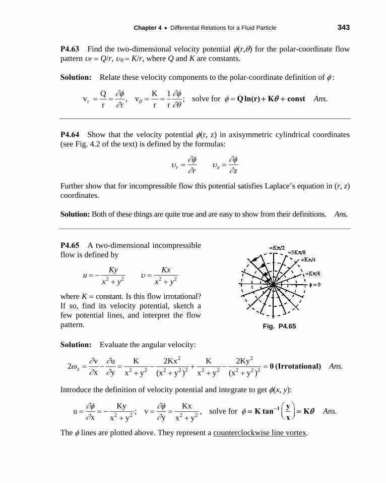
P4.65 A two-dimensional incompressible flow is defined by
2 2 2 2
Ky Kxu
x y x y
where K constant. Is this flow irrotational? If so, find its velocity potential, sketch a few potential lines, and interpret the flow pattern.
Fig. P4.65
Solution: Evaluate the angular velocity:
2 2
z 2 2 2 2 2 2 2 2 2 2
v u K 2Kx K 2Ky2 .
x y x y (x y ) x y (x y )Ans
0 (Irrotational)
Introduce the definition of velocity potential and integrate to get (x, y):
2 2 2 2
Ky Kxu ; v , solve for .
x yx y x yAns
1 y
K tan Kx
The lines are plotted above. They represent a counterclockwise line vortex.
344 Solutions Manual Fluid Mechanics, Fifth Edition
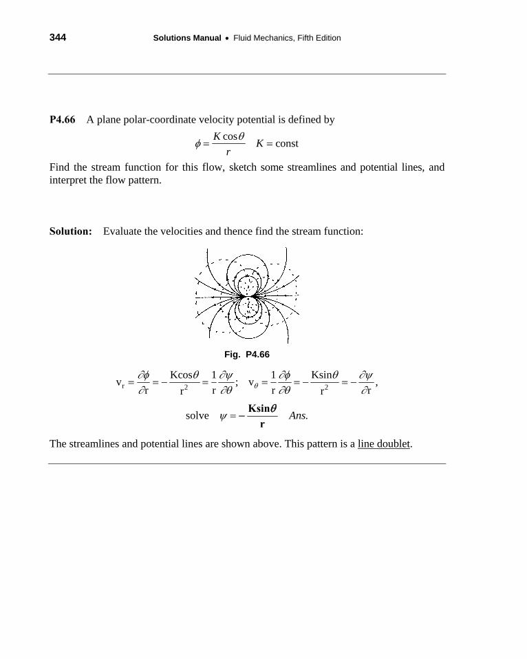
P4.66 A plane polar-coordinate velocity potential is defined by
cosconst
KK
r
Find the stream function for this flow, sketch some streamlines and potential lines, and interpret the flow pattern.
Solution: Evaluate the velocities and thence find the stream function:
Fig. P4.66
r 2 2
Kcos 1 1 Ksinv ; v ,
r r r rr r
solve .Ans
Ksin
r
The streamlines and potential lines are shown above. This pattern is a line doublet.
Chapter 4 Differential Relations for a Fluid Particle 345
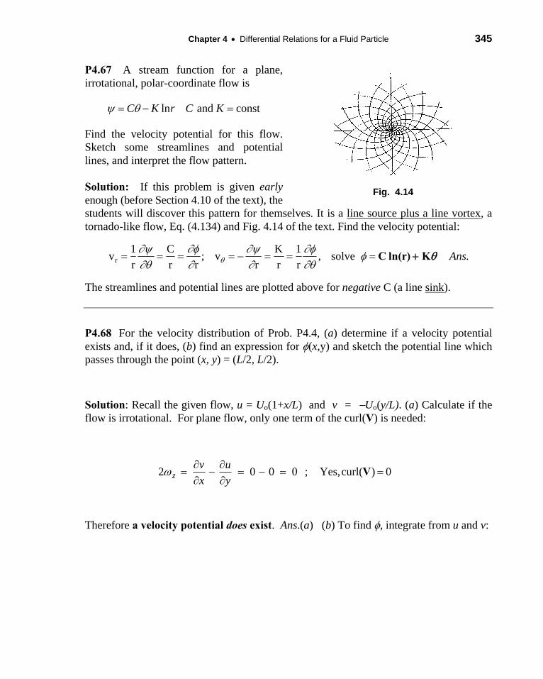
P4.67 A stream function for a plane, irrotational, polar-coordinate flow is
ln and constC K r C K
Find the velocity potential for this flow. Sketch some streamlines and potential lines, and interpret the flow pattern.
Solution: If this problem is given early enough (before Section 4.10 of the text), the
Fig. 4.14
students will discover this pattern for themselves. It is a line source plus a line vortex, a tornado-like flow, Eq. (4.134) and Fig. 4.14 of the text. Find the velocity potential:
r1 C K 1
v ; v , solve .r r r r r r
Ans
C ln(r) K
The streamlines and potential lines are plotted above for negative C (a line sink).
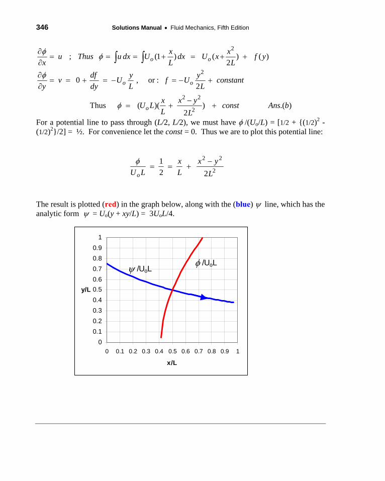
P4.68 For the velocity distribution of Prob. P4.4, (a) determine if a velocity potential exists and, if it does, (b) find an expression for (x,y) and sketch the potential line which passes through the point (x, y) = (L/2, L/2).
Solution: Recall the given flow, u = Uo(1+x/L) and v = Uo(y/L). (a) Calculate if the flow is irrotational. For plane flow, only one term of the curl(V) is needed:
Therefore a velocity potential does exist. Ans.(a) (b) To find , integrate from u and v:
0 )curl(Yes,;0002
Vy
u
x
vz
346 Solutions Manual Fluid Mechanics, Fifth Edition
For a potential line to pass through (L/2, L/2), we must have /(Uo/L) = [1/2 + {(1/2)2 -(1/2)2}/2] = ½. For convenience let the const = 0. Thus we are to plot this potential line:
The result is plotted (red) in the graph below, along with the (blue) line, which has the analytic form = Uo(y + xy/L) = 3UoL/4.
0
0.1
0.2
0.3
0.4
0.5
0.6
0.7
0.8
0.9
1
0 0.1 0.2 0.3 0.4 0.5 0.6 0.7 0.8 0.9 1
x/L
y/L
/UoL /UoL
2
2
2 2
2
; (1 ) ( ) ( )2
0 , or :2
Thus ( )( ) .( )2
o o
o o
o
x xu Thus u dx U dx U x f y
x L L
df y yv U f U constant
y dy L L
x yxU L const Ans b
L L
2
22
22
1
L
yx
L
x
LUo
Chapter 4 Differential Relations for a Fluid Particle 347
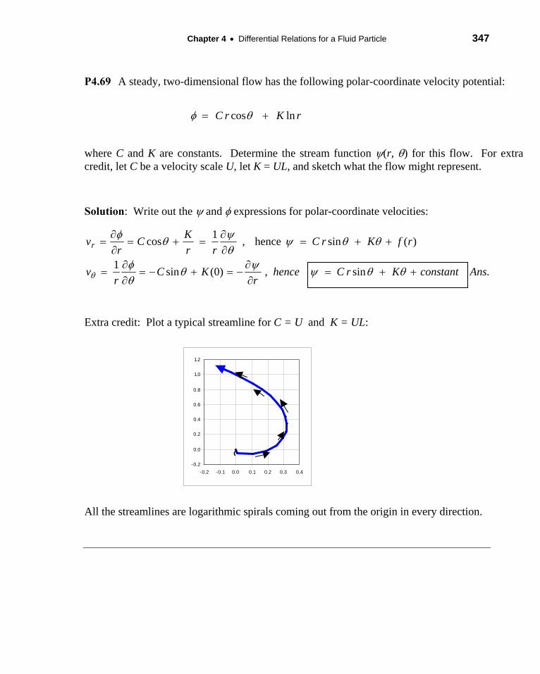
P4.69 A steady, two-dimensional flow has the following polar-coordinate velocity potential:
where C and K are constants. Determine the stream function (r, ) for this flow. For extra credit, let C be a velocity scale U, let K = UL, and sketch what the flow might represent.
Solution: Write out the and expressions for polar-coordinate velocities:
Extra credit: Plot a typical streamline for C = U and K = UL:
-0.2
0.0
0.2
0.4
0.6
0.8
1.0
1.2
-0.2 -0.1 0.0 0.1 0.2 0.3 0.4
O
All the streamlines are logarithmic spirals coming out from the origin in every direction.
rKrC lncos
.sin,)0(sin1
)(sinhence,1
cos
AnsconstantKrChencer
KCr
v
rfKrCrr
KC
rvr
348 Solutions Manual Fluid Mechanics, Fifth Edition
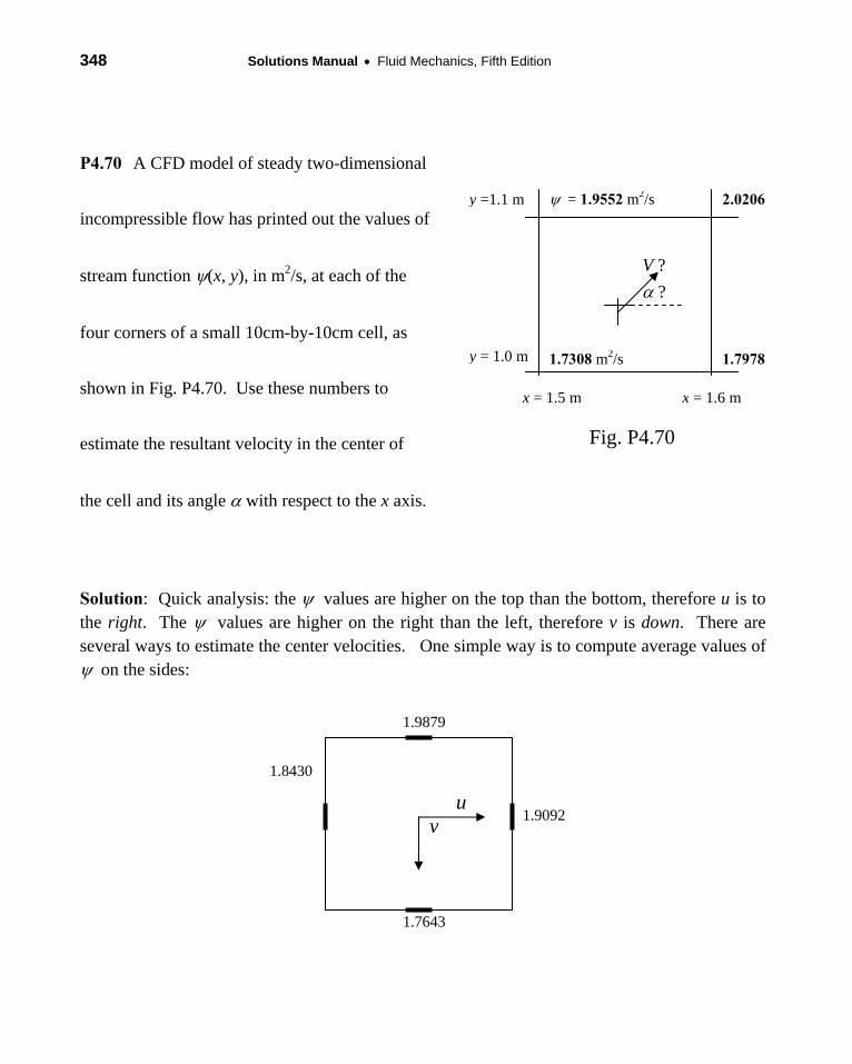
P4.70 A CFD model of steady two-dimensional
incompressible flow has printed out the values of
stream function (x, y), in m2/s, at each of the
four corners of a small 10cm-by-10cm cell, as
shown in Fig. P4.70. Use these numbers to
estimate the resultant velocity in the center of
the cell and its angle with respect to the x axis.
Solution: Quick analysis: the values are higher on the top than the bottom, therefore u is to the right. The values are higher on the right than the left, therefore v is down. There are several ways to estimate the center velocities. One simple way is to compute average values of on the sides:
x = 1.5 m x = 1.6 m
y = 1.0 m
y =1.1 m
?
V ?
= 1.9552 m2/s 2.0206
1.79781.7308 m2/s
Fig. P4.70
uv
1.9879
1.9092
1.7643
1.8430
Chapter 4 Differential Relations for a Fluid Particle 349
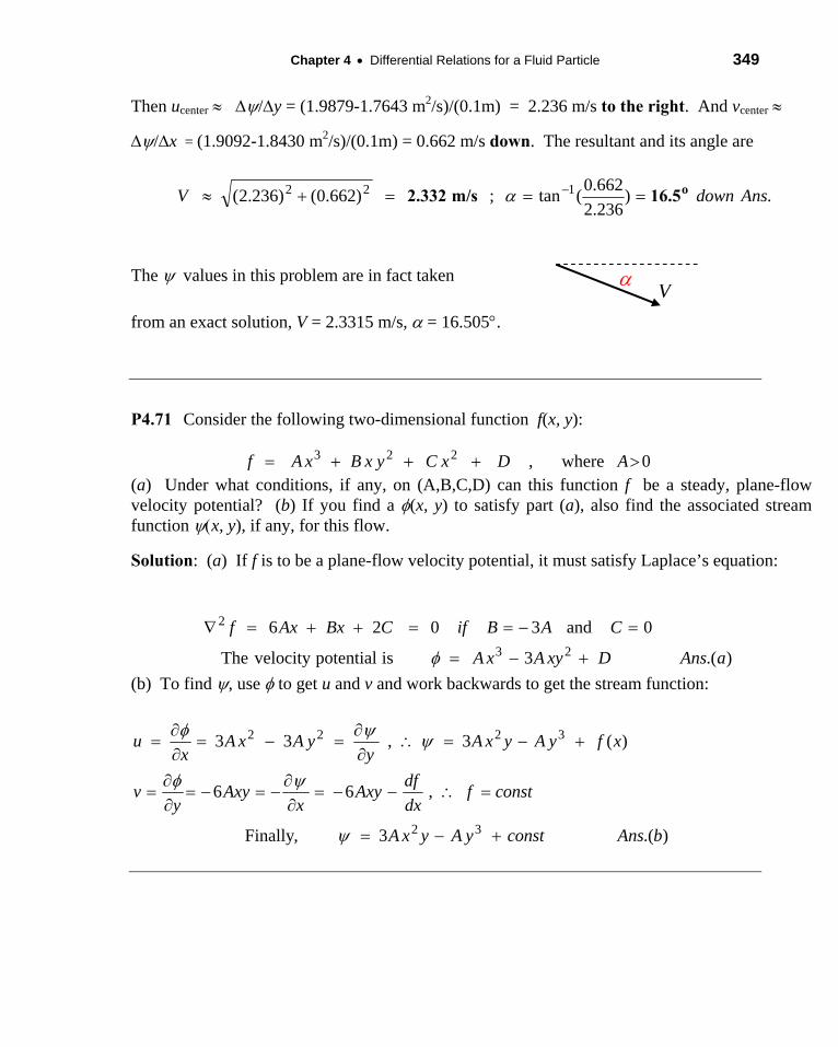
Then ucenter /y = (1.9879-1.7643 m2/s)/(0.1m) = 2.236 m/s to the right. And vcenter
/x = (1.9092-1.8430 m2/s)/(0.1m) = 0.662 m/s down. The resultant and its angle are
The values in this problem are in fact taken
from an exact solution, V = 2.3315 m/s, = 16.505.
P4.71 Consider the following two-dimensional function f(x, y):
(a) Under what conditions, if any, on (A,B,C,D) can this function f be a steady, plane-flow velocity potential? (b) If you find a (x, y) to satisfy part (a), also find the associated stream function x, y), if any, for this flow.
Solution: (a) If f is to be a plane-flow velocity potential, it must satisfy Laplace’s equation:
(b) To find , use to get u and v and work backwards to get the stream function:
.)236.2
662.0(tan;)662.0()236.2( 122 AnsdownV o16.5m/s2.332
V
0where,223 ADxCyxBxAf
).(3ispotentialvelocityThe
0and302623
2
aAnsDxyAxA
CABifCBxAxf
).(3,Finally
,66
)(3,33
32
3222
bAnsconstyAyxA
constfdx
dfAxy
xAxy
yv
xfyAyxAy
yAxAx
u
350 Solutions Manual Fluid Mechanics, Fifth Edition
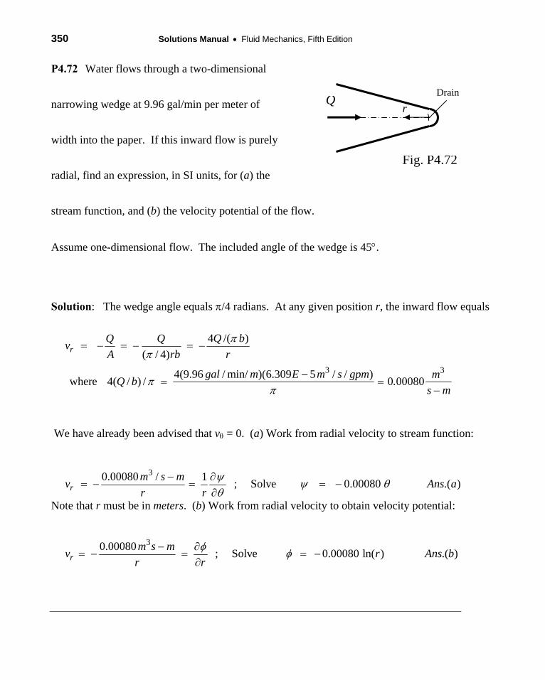
P4.72 Water flows through a two-dimensional
narrowing wedge at 9.96 gal/min per meter of
width into the paper. If this inward flow is purely
radial, find an expression, in SI units, for (a) the
stream function, and (b) the velocity potential of the flow.
Assume one-dimensional flow. The included angle of the wedge is 45.
Solution: The wedge angle equals /4 radians. At any given position r, the inward flow equals
We have already been advised that v = 0. (a) Work from radial velocity to stream function:
Note that r must be in meters. (b) Work from radial velocity to obtain velocity potential:
r Q
Drain
Fig. P4.72
3 3
4 /( )
( / 4)
4(9.96 / min/ )(6.309 5 / / )where 4( / ) / 0 00080
rQ bQ Q
vA rb r
gal m E m s gpm mQ b .
s m
30.00080 / 1; Solve 0.00080 .( )
rm s m
v Ans ar r
30.00080; Solve 0.00080 ln( ) .( )
rm s m
v r Ans br r
Chapter 4 Differential Relations for a Fluid Particle 351
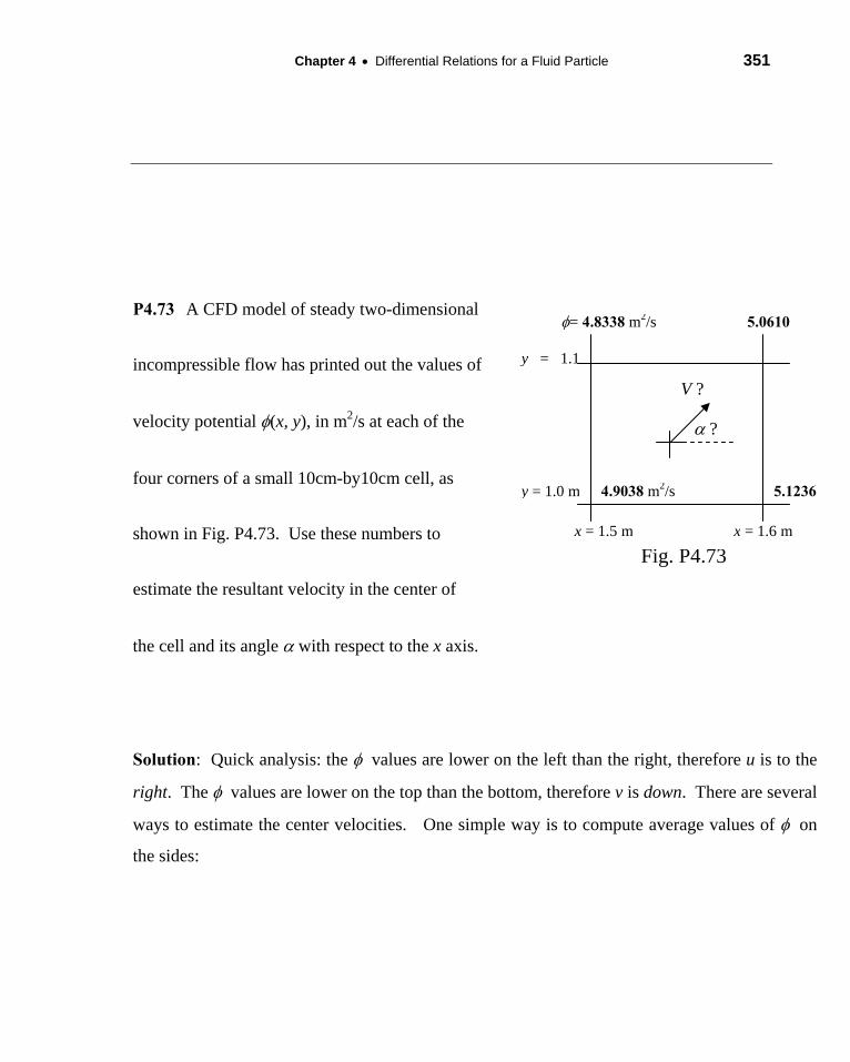
P4.73 A CFD model of steady two-dimensional
incompressible flow has printed out the values of
velocity potential (x, y), in m2/s at each of the
four corners of a small 10cm-by10cm cell, as
shown in Fig. P4.73. Use these numbers to
estimate the resultant velocity in the center of
the cell and its angle with respect to the x axis.
Solution: Quick analysis: the values are lower on the left than the right, therefore u is to the
right. The values are lower on the top than the bottom, therefore v is down. There are several
ways to estimate the center velocities. One simple way is to compute average values of on
the sides:
x = 1.5 m x = 1.6 m
y = 1.0 m
y = 1.1
?
V ?
= 4.8338 m2/s 5.0610
5.12364.9038 m2/s
Fig. P4.73
352 Solutions Manual Fluid Mechanics, Fifth Edition
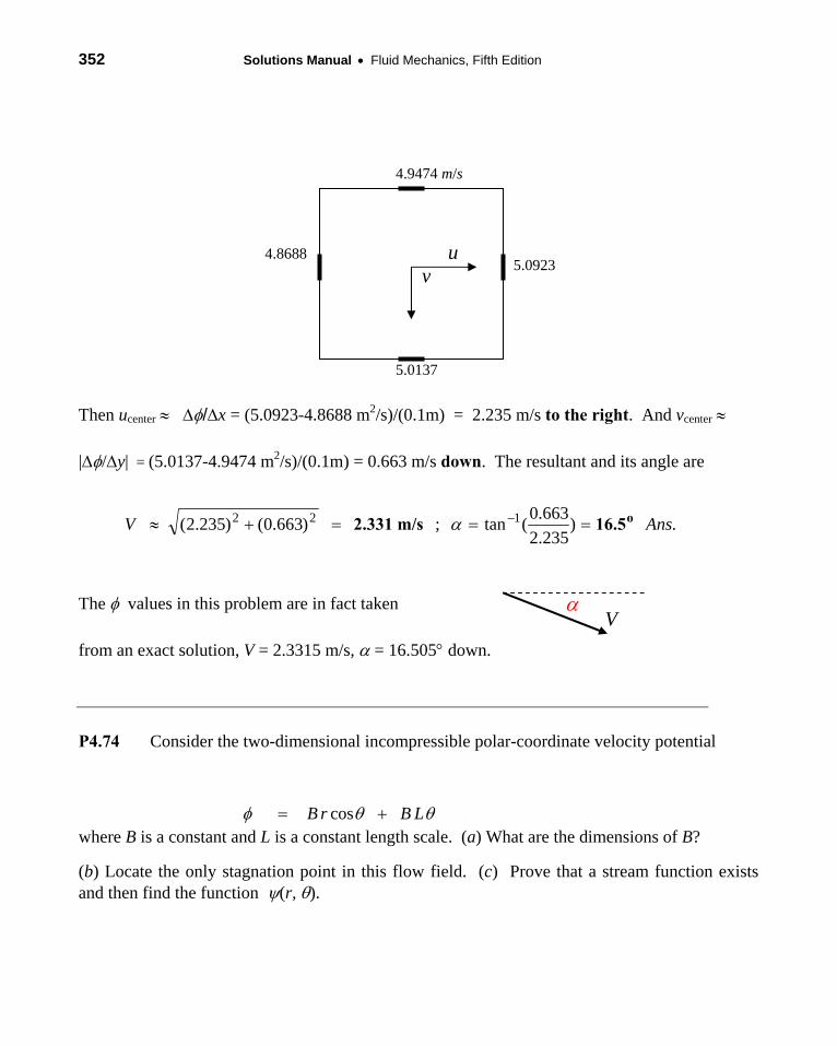
Then ucenter /x = (5.0923-4.8688 m2/s)/(0.1m) = 2.235 m/s to the right. And vcenter
|/y| = (5.0137-4.9474 m2/s)/(0.1m) = 0.663 m/s down. The resultant and its angle are
The values in this problem are in fact taken
from an exact solution, V = 2.3315 m/s, = 16.505 down.
P4.74 Consider the two-dimensional incompressible polar-coordinate velocity potential
where B is a constant and L is a constant length scale. (a) What are the dimensions of B?
(b) Locate the only stagnation point in this flow field. (c) Prove that a stream function exists and then find the function (r, ).
uv
4.9474 m/s
5.0923
5.0137
4.8688
.)235.2
663.0(tan;)663.0()235.2( 122 AnsV o16.5m/s2.331
V
LBrB cos
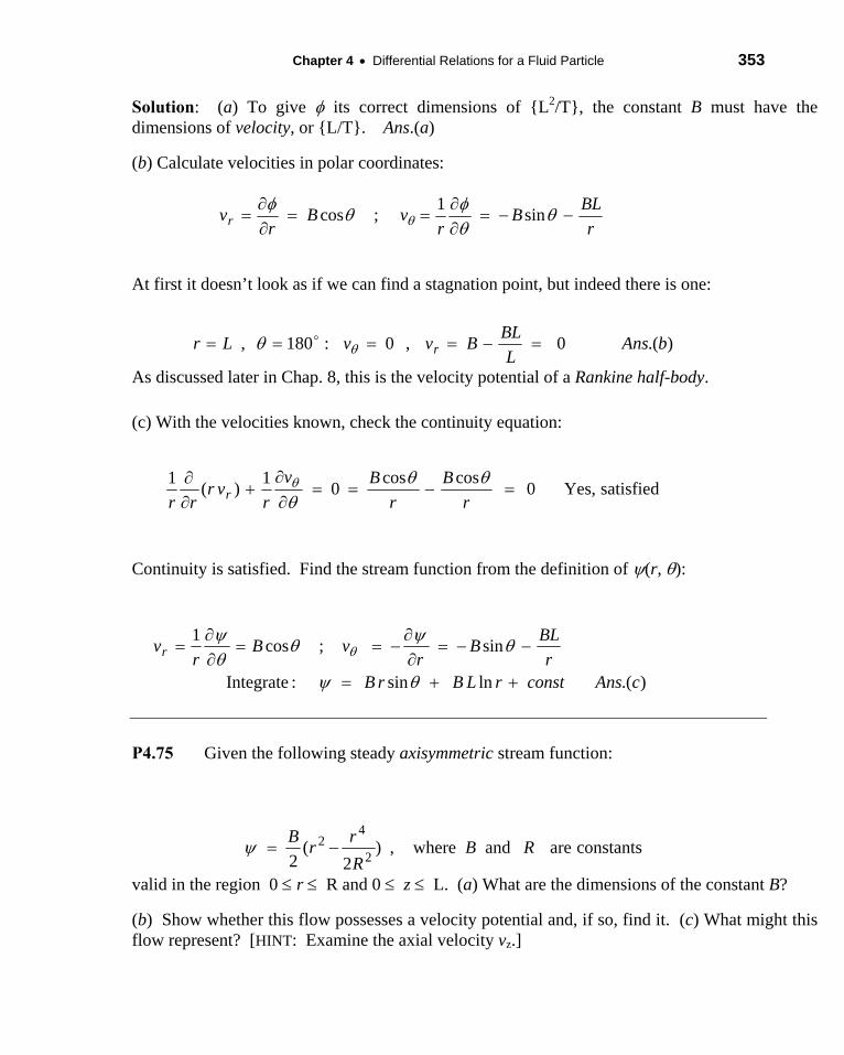
Chapter 4 Differential Relations for a Fluid Particle 353
Solution: (a) To give its correct dimensions of {L2/T}, the constant B must have the dimensions of velocity, or {L/T}. Ans.(a)
(b) Calculate velocities in polar coordinates:
At first it doesn’t look as if we can find a stagnation point, but indeed there is one:
As discussed later in Chap. 8, this is the velocity potential of a Rankine half-body.
(c) With the velocities known, check the continuity equation:
Continuity is satisfied. Find the stream function from the definition of (r, ):
P4.75 Given the following steady axisymmetric stream function:
valid in the region 0 r R and 0 z L. (a) What are the dimensions of the constant B?
(b) Show whether this flow possesses a velocity potential and, if so, find it. (c) What might this flow represent? [HINT: Examine the axial velocity vz.]
r
BLB
rvB
rvr
sin1
;cos
).(0,0:180, bAnsL
BLBvvLr r
satisfiedYes,0coscos
01
)(1
r
B
r
Bv
rvr
rr r
).(lnsin:Integrate
sin;cos1
cAnsconstrLBrBr
BLB
rvB
rvr
constantsareandwhere,)2
(2 2
42 RB
R
rr
B
354 Solutions Manual Fluid Mechanics, Fifth Edition
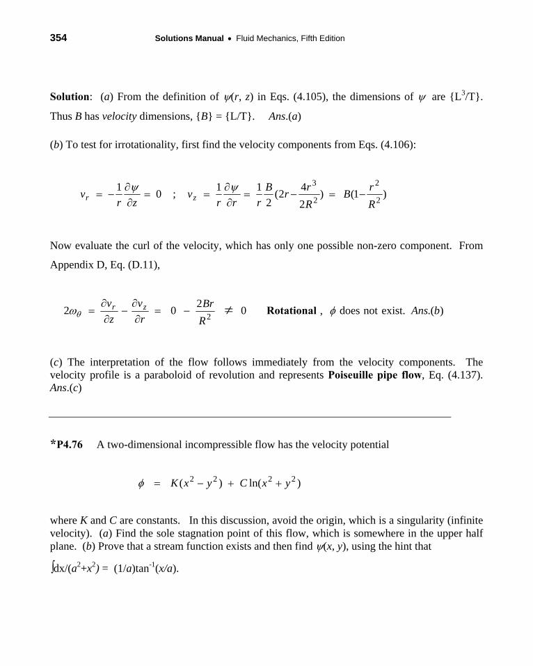
Solution: (a) From the definition of (r, z) in Eqs. (4.105), the dimensions of are {L3/T}.
Thus B has velocity dimensions, {B} = {L/T}. Ans.(a)
(b) To test for irrotationality, first find the velocity components from Eqs. (4.106):
Now evaluate the curl of the velocity, which has only one possible non-zero component. From
Appendix D, Eq. (D.11),
(c) The interpretation of the flow follows immediately from the velocity components. The velocity profile is a paraboloid of revolution and represents Poiseuille pipe flow, Eq. (4.137). Ans.(c)
*P4.76 A two-dimensional incompressible flow has the velocity potential
where K and C are constants. In this discussion, avoid the origin, which is a singularity (infinite velocity). (a) Find the sole stagnation point of this flow, which is somewhere in the upper half plane. (b) Prove that a stream function exists and then find (x, y), using the hint that
dx/(a2+x2) = (1/a)tan-1(x/a).
)1()2
42(
2
11;0
12
2
2
3
R
rB
R
rr
B
rrrv
zrv zr
).(.existnotdoes,02
022
bAnsR
Br
r
v
z
v zr Rotational
)ln()( 2222 yxCyxK
Chapter 4 Differential Relations for a Fluid Particle 355
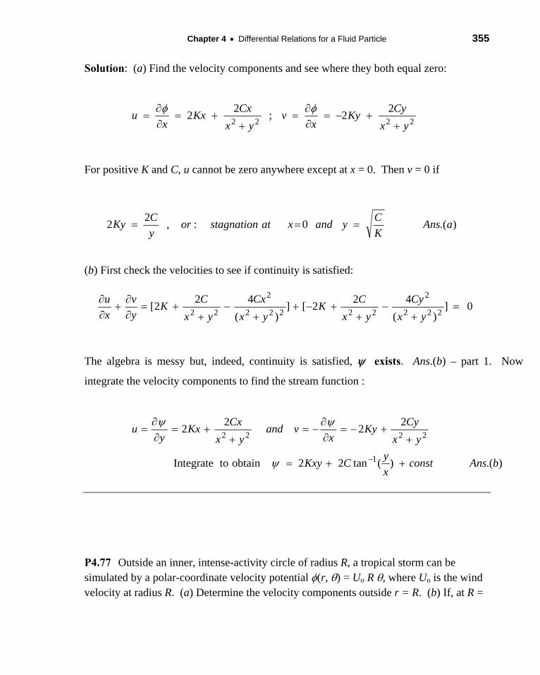
Solution: (a) Find the velocity components and see where they both equal zero:
For positive K and C, u cannot be zero anywhere except at x = 0. Then v = 0 if
(b) First check the velocities to see if continuity is satisfied:
The algebra is messy but, indeed, continuity is satisfied, exists. Ans.(b) – part 1. Now
integrate the velocity components to find the stream function :
P4.77 Outside an inner, intense-activity circle of radius R, a tropical storm can be simulated by a polar-coordinate velocity potential (r, ) = Uo R , where Uo is the wind velocity at radius R. (a) Determine the velocity components outside r = R. (b) If, at R =
2222
22;
22
yx
CyKy
xv
yx
CxKx
xu
).(0:,2
2 aAnsK
Cyandxatstagnationor
y
CKy
0])(
422[]
)(
422[
222
2
22222
2
22
yx
Cy
yx
CK
yx
Cx
yx
CK
y
v
x
u
).()(tan22obtaintoIntegrate
22
22
1
2222
bAnsconstx
yCKxy
yx
CyKy
xvand
yx
CxKx
yu
356 Solutions Manual Fluid Mechanics, Fifth Edition
25 mi, the velocity is 100 mi/h and the pressure 99 kPa, calculate the velocity and pressure at r = 100 mi.
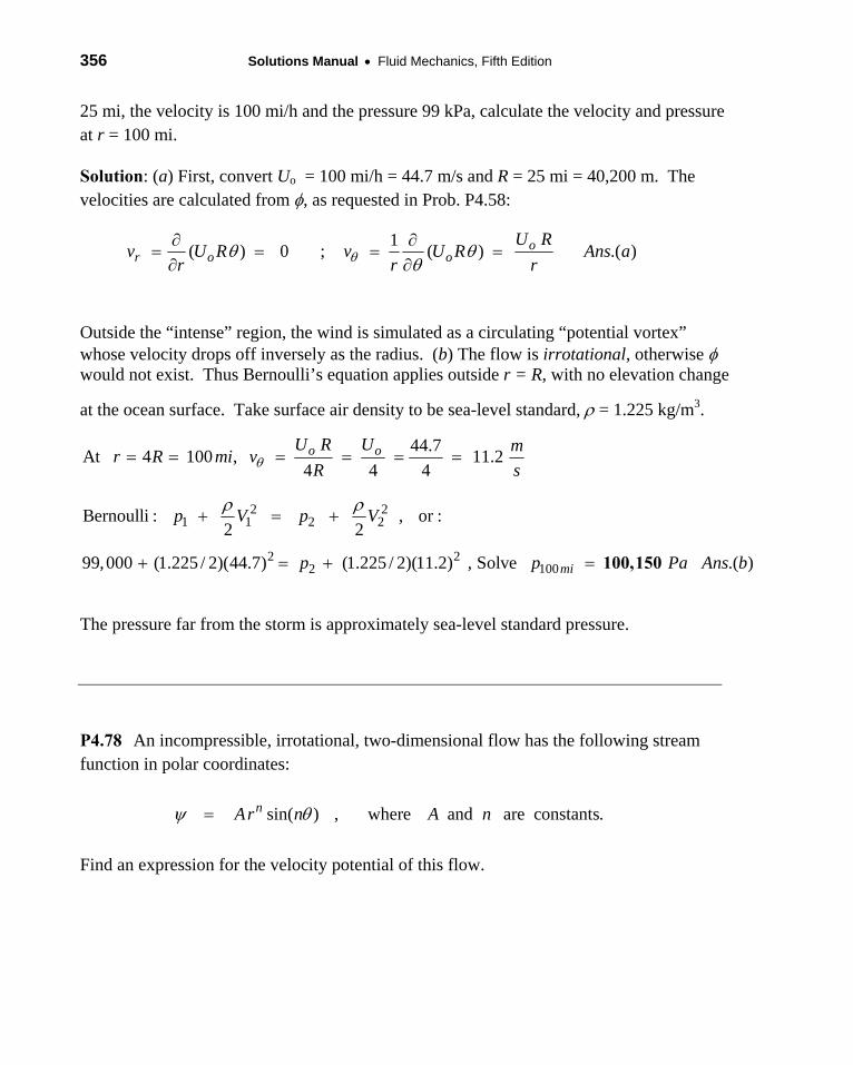
Solution: (a) First, convert Uo = 100 mi/h = 44.7 m/s and R = 25 mi = 40,200 m. The velocities are calculated from , as requested in Prob. P4.58:
1
( ) 0 ; ( ) .( )or o o
U Rv U R v U R Ans a
r r r
Outside the “intense” region, the wind is simulated as a circulating “potential vortex” whose velocity drops off inversely as the radius. (b) The flow is irrotational, otherwise would not exist. Thus Bernoulli’s equation applies outside r = R, with no elevation change
at the ocean surface. Take surface air density to be sea-level standard, = 1.225 kg/m3.
44.7At 4 100 , 11.2
4 4 4o oU R U m
r R mi vR s
2 21 1 2 2Bernoulli : , or :
2 2p V p V
2 2
2 10099,000 (1.225 / 2)(44.7) (1.225 / 2)(11.2) , Solve .( )mip p Pa Ans b 100,150
The pressure far from the storm is approximately sea-level standard pressure.
P4.78 An incompressible, irrotational, two-dimensional flow has the following stream function in polar coordinates:
sin( ) , where and are constants.nAr n A n
Find an expression for the velocity potential of this flow.
Chapter 4 Differential Relations for a Fluid Particle 357
Solution: Use to find the velocity components, then integrate back to find .
1
1
1cos( ) ; Integrate : cos( ) ( )
1 1sin( ) [ sin( )]
Compare : 0 , and thus cos( ) constant .
n nr
n n
n
v n Ar n Ar n fr r
dfv n Ar n nAr n
r r r ddf
Ar n Ansd
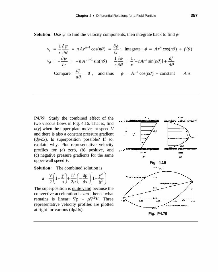
P4.79 Study the combined effect of the two viscous flows in Fig. 4.16. That is, find u(y) when the upper plate moves at speed V and there is also a constant pressure gradient (dp/dx). Is superposition possible? If so, explain why. Plot representative velocity profiles for (a) zero, (b) positive, and (c) negative pressure gradients for the same upper-wall speed V.
Fig. 4.16
Solution: The combined solution is 2 2
2
V y h dp yu 1 1
2 h 2 dx h
The superposition is quite valid because the convective acceleration is zero, hence what remains is linear: p 2V. Three representative velocity profiles are plotted at right for various (dp/dx).
Fig. P4.79
358 Solutions Manual Fluid Mechanics, Fifth Edition
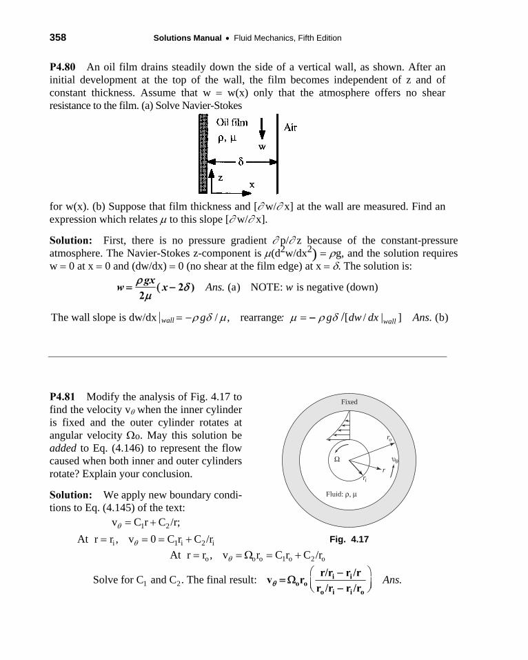
P4.80 An oil film drains steadily down the side of a vertical wall, as shown. After an initial development at the top of the wall, the film becomes independent of z and of constant thickness. Assume that w w(x) only that the atmosphere offers no shear resistance to the film. (a) Solve Navier-Stokes
for w(x). (b) Suppose that film thickness and [ w/ x] at the wall are measured. Find an expression which relates to this slope [ w/ x].
Solution: First, there is no pressure gradient p/ z because of the constant-pressure atmosphere. The Navier-Stokes z-component is (d2w/dx2) g, and the solution requires w 0 at x 0 and (dw/dx) 0 (no shear at the film edge) at x . The solution is:
. (a) NOTE: is negative (down)Ans wgx
w x
2 )2
The wall slope is dw/dx / , rearrange [ / | ] . (b)/wall wallg : g dw dx Ans
P4.81 Modify the analysis of Fig. 4.17 to find the velocity v when the inner cylinder is fixed and the outer cylinder rotates at angular velocity o. May this solution be added to Eq. (4.146) to represent the flow caused when both inner and outer cylinders rotate? Explain your conclusion.
Solution: We apply new boundary condi-tions to Eq. (4.145) of the text:
1 2
i 1 i 2 i
v C r C /r;
At r r , v 0 C r C /r
Fixed
Fluid: ρ, μ
ro
ri
υr
Ω θ
Fig. 4.17
o o o 1 o 2 oAt r r , v r C r C /r
1 2Solve for C and C . The final result: .Ans
i io o
o i i o
r/r r /rv r
r /r r /r
Chapter 4 Differential Relations for a Fluid Particle 359
This solution may indeed be added to the inner-rotation solution, Eq. (4.146), because the convective acceleration is zero and hence the Navier-Stokes equation is linear.
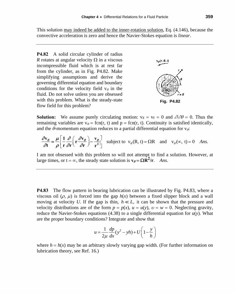
P4.82 A solid circular cylinder of radius R rotates at angular velocity in a viscous incompressible fluid which is at rest far from the cylinder, as in Fig. P4.82. Make simplifying assumptions and derive the governing differential equation and boundary conditions for the velocity field v in the fluid. Do not solve unless you are obsessed with this problem. What is the steady-state flow field for this problem?
Fig. P4.82
Solution: We assume purely circulating motion: vz vr 0 and / 0. Thus the remaining variables are v fcn(r, t) and p fcn(r, t). Continuity is satisfied identically, and the -momentum equation reduces to a partial differential equation for v:
subject to v (R, t) R and v ( , t) 0 .Ans
2
v v v1r
t r r r r
I am not obsessed with this problem so will not attempt to find a solution. However, at large times, or t , the steady state solution is v R2/r. Ans.
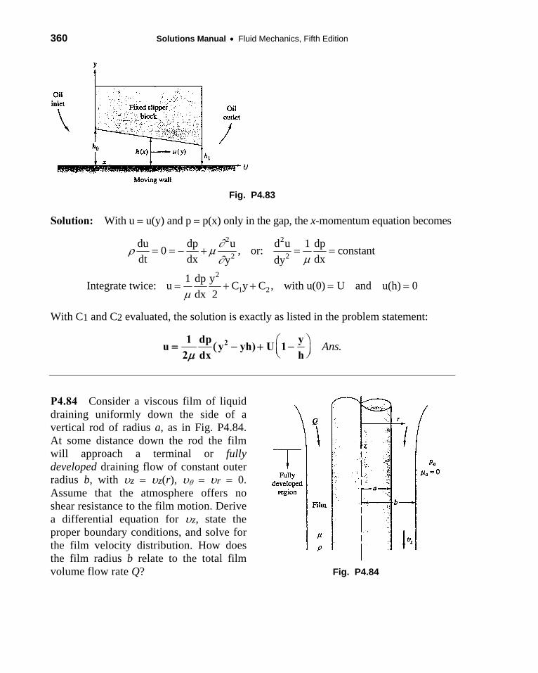
P4.83 The flow pattern in bearing lubrication can be illustrated by Fig. P4.83, where a viscous oil (, ) is forced into the gap h(x) between a fixed slipper block and a wall moving at velocity U. If the gap is thin, ,h L it can be shown that the pressure and velocity distributions are of the form p p(x), u u(y), w 0. Neglecting gravity, reduce the Navier-Stokes equations (4.38) to a single differential equation for u(y). What are the proper boundary conditions? Integrate and show that
21( ) 1
2
dp yu y yh U
dx h
where h h(x) may be an arbitrary slowly varying gap width. (For further information on lubrication theory, see Ref. 16.)
360 Solutions Manual Fluid Mechanics, Fifth Edition
Fig. P4.83
Solution: With u u(y) and p p(x) only in the gap, the x-momentum equation becomes
2 2
2 2
du dp u d u 1 dp0 , or: constant
dt dx dxy dy
2
1 21 dp y
Integrate twice: u C y C , with u(0) U and u(h) 0dx 2
With C1 and C2 evaluated, the solution is exactly as listed in the problem statement:
.Ans
21 dp yu y yh) U 1
2 dx h
P4.84 Consider a viscous film of liquid draining uniformly down the side of a vertical rod of radius a, as in Fig. P4.84. At some distance down the rod the film will approach a terminal or fully developed draining flow of constant outer radius b, with z z(r), r 0. Assume that the atmosphere offers no shear resistance to the film motion. Derive a differential equation for z, state the proper boundary conditions, and solve for the film velocity distribution. How does the film radius b relate to the total film volume flow rate Q?
Fig. P4.84
Chapter 4 Differential Relations for a Fluid Particle 361
Solution: With vz fcn(r) only, the Navier-Stokes z-momentum relation is
2zz
dv p0 g v ,
dt z
2z
z 1 21 d dv g gr
or: r , Integrate twice: v C ln(r) Cr dr dr 4
zvThe proper B.C. are: u(a) 0 (no-slip) and (b) 0 (no free-surface shear stress)
r
The final solution is .Ans
22 2
zgb r g
v ln r a2 a 4
b
za
The flow rate is Q v 2 r dr
bwhere .
aAns
44 2 4ga
3 1 4 4 ln ,8
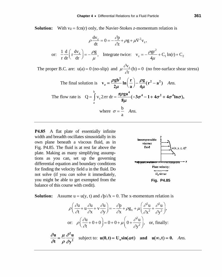
P4.85 A flat plate of essentially infinite width and breadth oscillates sinusoidally in its own plane beneath a viscous fluid, as in Fig. P4.85. The fluid is at rest far above the plate. Making as many simplifying assump-tions as you can, set up the governing differential equation and boundary conditions for finding the velocity field u in the fluid. Do not solve (if you can solve it immediately, you might be able to get exempted from the balance of this course with credit).
Fig. P4.85
Solution: Assume u u(y, t) and p/x 0. The x-momentum relation is
2 2
x 2 2
u u u p u uu v g ,
t x y x x y
2
2
u uor: 0 0 0 0 0 , or, finally:
t y
subject to: .Ans
2
o2
u uu(0, t) U sin t and u , t 0.
t y
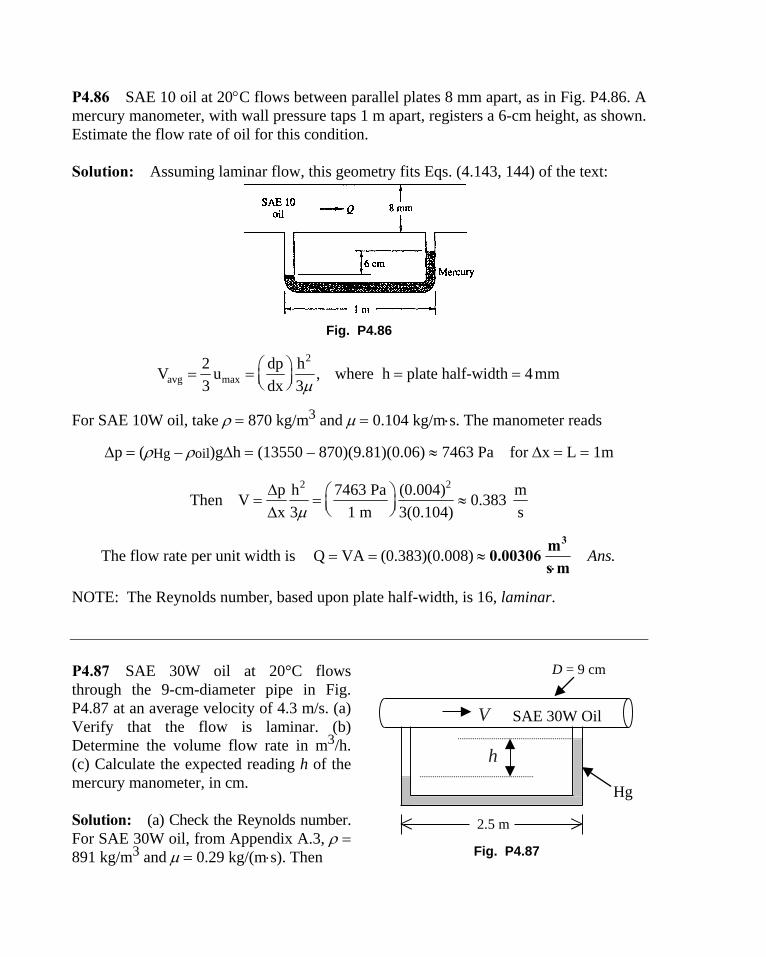
P4.86 SAE 10 oil at 20C flows between parallel plates 8 mm apart, as in Fig. P4.86. A mercury manometer, with wall pressure taps 1 m apart, registers a 6-cm height, as shown. Estimate the flow rate of oil for this condition.
Solution: Assuming laminar flow, this geometry fits Eqs. (4.143, 144) of the text:
Fig. P4.86
2
avg max2 dp h
V u , where h plate half-width 4mm3 dx 3
For SAE 10W oil, take 870 kg/m3 and 0.104 kg/ms. The manometer reads
p (Hg – oil)gh (13550 – 870)(9.81)(0.06) 7463 Pa for x L 1m
2 2p h 7463 Pa (0.004) mThen V 0.383
x 3 1 m 3(0.104) s
The flow rate per unit width is Q VA (0.383)(0.008) .Ans 3m
0.00306 s m
NOTE: The Reynolds number, based upon plate half-width, is 16, laminar.
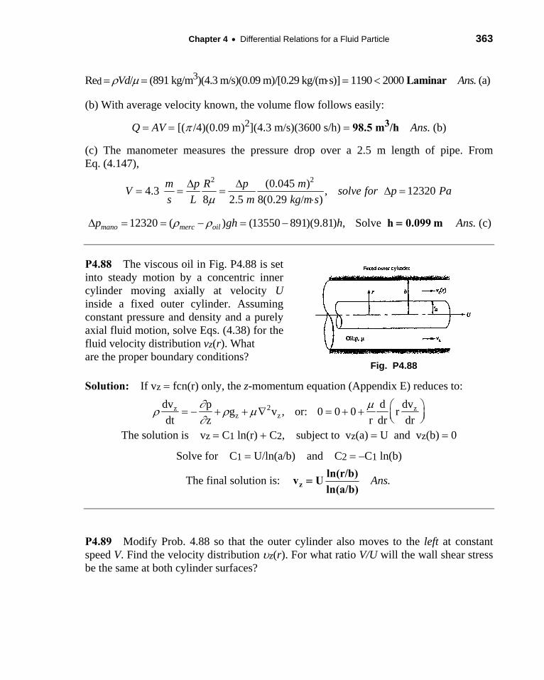
P4.87 SAE 30W oil at 20°C flows through the 9-cm-diameter pipe in Fig. P4.87 at an average velocity of 4.3 m/s. (a) Verify that the flow is laminar. (b) Determine the volume flow rate in m3/h. (c) Calculate the expected reading h of the mercury manometer, in cm.
Solution: (a) Check the Reynolds number. For SAE 30W oil, from Appendix A.3, 891 kg/m3 and 0.29 kg/(ms). Then
2.5 m
D = 9 cm
Hg
SAE 30W Oil
h
V
Fig. P4.87
Chapter 4 Differential Relations for a Fluid Particle 363
Red Vd/ (891 kg/m3)(4.3 m/s)(0.09 m)/[0.29 kg/(ms)] 1190 2000 Laminar Ans. (a)
(b) With average velocity known, the volume flow follows easily:
Q AV [(/4)(0.09 m)2](4.3 m/s)(3600 s/h) 98.5 m3/h Ans. (b)
(c) The manometer measures the pressure drop over a 2.5 m length of pipe. From Eq. (4.147),
2 2(0.045 )4.3 , 12320
8 2.5 8(0.29 / )
m p R p mV solve for p Pa
s L m kg m s
12320 ( ) (13550 891)(9.81) , Solvemano merc oilp gh h h 0.099 m Ans. (c)
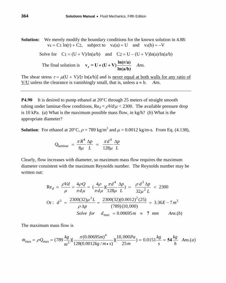
P4.88 The viscous oil in Fig. P4.88 is set into steady motion by a concentric inner cylinder moving axially at velocity U inside a fixed outer cylinder. Assuming constant pressure and density and a purely axial fluid motion, solve Eqs. (4.38) for the fluid velocity distribution vz(r). What are the proper boundary conditions?
Fig. P4.88
Solution: If vz fcn(r) only, the z-momentum equation (Appendix E) reduces to:
2z zz z
dv p d dvg v , or: 0 0 0 r
dt z r dr dr
The solution is vz C1 ln(r) C2, subject to vz(a) U and vz(b) 0
Solve for C1 U/ln(a/b) and C2 –C1 ln(b)
The final solution is: .Anszln(r/b)
v Uln(a/b)
P4.89 Modify Prob. 4.88 so that the outer cylinder also moves to the left at constant speed V. Find the velocity distribution z(r). For what ratio V/U will the wall shear stress be the same at both cylinder surfaces?
364 Solutions Manual Fluid Mechanics, Fifth Edition
Solution: We merely modify the boundary conditions for the known solution in 4.88: vz C1 ln(r) C2, subject to vz(a) U and vz(b) –V
Solve for C1 (U V)/ln(a/b) and C2 U – (U V)ln(a)/ln(a/b)
The final solution is = zln(r/a)
v U (U V)ln(a/b)
Ans.
The shear stress (U V)/[r ln(a/b)] and is never equal at both walls for any ratio of V/U unless the clearance is vanishingly small, that is, unless a b. Ans.
P4.90 It is desired to pump ethanol at 20C through 25 meters of straight smooth tubing under laminar-flow conditions, Red = Vd/ < 2300. The available pressure drop is 10 kPa. (a) What is the maximum possible mass flow, in kg/h? (b) What is the appropriate diameter?
Solution: For ethanol at 20C, = 789 kg/m3 and = 0.0012 kg/m-s. From Eq. (4.138),
4 4
laminar 8 128
R p d pQ
L L
Clearly, flow increases with diameter, so maximum mass flow requires the maximum diameter consistent with the maximum Reynolds number. The Reynolds number may be written out:
34
2
2 23 3
max
4 4Re ( )( ) 2300
128 32
2300(32) 2300(32)(0.0012) (25)Or : 3.36 7
(789) (10,000)
0.00695 .( )
dd pVd Q d p
d d L L
Ld E m
p
Solve for d m mm Ans b
7
The maximum mass flow is
4
max max 3
(0.00695 ) 10,000(789 )[ ]( ) 0.0151 .( )
128(0.0012 / ) 25
kg m Pa kg kgm Q Ans a
kg m s m s hm
54
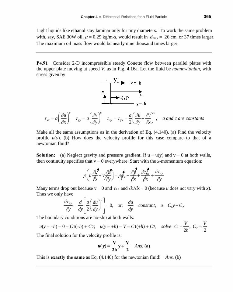
Chapter 4 Differential Relations for a Fluid Particle 365
Light liquids like ethanol stay laminar only for tiny diameters. To work the same problem with, say, SAE 30W oil, = 0.29 kg/m-s, would result in dmax = 26 cm, or 37 times larger. The maximum oil mass flow would be nearly nine thousand times larger.
P4.91 Consider 2-D incompressible steady Couette flow between parallel plates with the upper plate moving at speed V, as in Fig. 4.16a. Let the fluid be nonnewtonian, with stress given by
,2
c c c
xx yy xy yxu v a u v
a ax y y x
a and c are constants
Make all the same assumptions as in the derivation of Eq. (4.140). (a) Find the velocity profile u(y). (b) How does the velocity profile for this case compare to that of a newtonian fluid?
Solution: (a) Neglect gravity and pressure gradient. If u u(y) and v 0 at both walls, then continuity specifies that v 0 everywhere. Start with the x-momentum equation:
xyxxx
u u pu v g
x y x x y
Many terms drop out because v 0 and xx and u/x 0 (because u does not vary with x). Thus we only have
1 20, : ,2
cxy d a du du
or constant u C y Cy dy dy dy
The boundary conditions are no-slip at both walls:
u(y –h) 0 C1(–h) C2; u(y h) V C1(h) C2, solve 1 2,2 2
V VC C
h
The final solution for the velocity profile is:
. (a)Ansu yV V
( ) y2h 2
This is exactly the same as Eq. (4.140) for the newtonian fluid! Ans. (b)
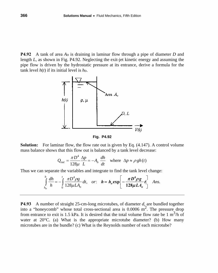
366 Solutions Manual Fluid Mechanics, Fifth Edition
P4.92 A tank of area Ao is draining in laminar flow through a pipe of diameter D and length L, as shown in Fig. P4.92. Neglecting the exit-jet kinetic energy and assuming the pipe flow is driven by the hydrostatic pressure at its entrance, derive a formula for the tank level h(t) if its initial level is ho.
Fig. P4.92
Solution: For laminar flow, the flow rate out is given by Eq. (4.147). A control volume mass balance shows that this flow out is balanced by a tank level decrease:
4
where ( )128out o
D p dhQ A p gh t
L dt
Thus we can separate the variables and integrate to find the tank level change: 4
0
, : .128
o
h t
oh
dh D gdt or Ans
h LA
o
o
D gh h t
LA
4
exp128
P4.93 A number of straight 25-cm-long microtubes, of diameter d, are bundled together into a “honeycomb” whose total cross-sectional area is 0.0006 m2. The pressure drop from entrance to exit is 1.5 kPa. It is desired that the total volume flow rate be 1 m3/h of water at 20°C. (a) What is the appropriate microtube diameter? (b) How many microtubes are in the bundle? (c) What is the Reynolds number of each microtube?
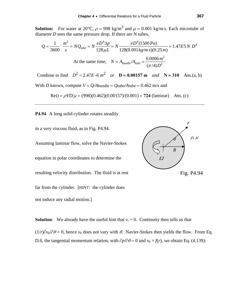
Chapter 4 Differential Relations for a Fluid Particle 367
Solution: For water at 20°C, 998 kg/m3 and 0.001 kg/ms. Each microtube of diameter D sees the same pressure drop. If there are N tubes,
3 4 441 (1500 )
1.47 5 3600 128 128(0.001 / )(0.25 )tube
m D p D PaQ NQ N N E N D
s L kg m s m
2
2
0.0006At the same time, /
( /4)bundle tube
mN A A
D
Combine to find D2 2.47E6 m2 or D 0.00157 m and N 310 Ans.(a, b)
With D known, compute V Q/Abundle Qtube/Atube 0.462 m/s and
ReD VD/ (998)(0.462)(0.00157)/(0.001) 724 (laminar) Ans. (c)
P4.94 A long solid cylinder rotates steadily
in a very viscous fluid, as in Fig. P4.94.
Assuming laminar flow, solve the Navier-Stokes
equation in polar coordinates to determine the
resulting velocity distribution. The fluid is at rest
far from the cylinder. [HINT: the cylinder does
not induce any radial motion.]
Solution: We already have the useful hint that vr = 0. Continuity then tells us that
(1/r)v/ = 0, hence v does not vary with . Navier-Stokes then yields the flow. From Eq.
D.6, the tangential momentum relation, with p/0 and v = f(r), we obtain Eq. (4.139):
R
r
Fig. P4.94
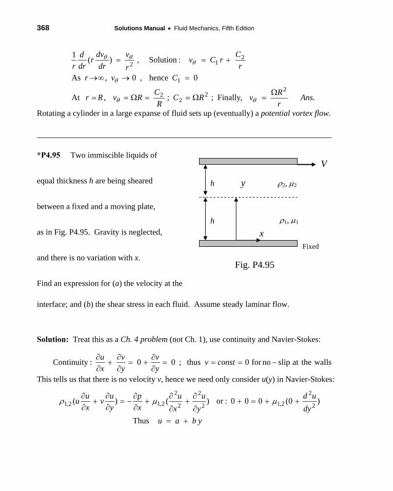
368 Solutions Manual Fluid Mechanics, Fifth Edition
Rotating a cylinder in a large expanse of fluid sets up (eventually) a potential vortex flow.
________________________________________________________________________
*P4.95 Two immiscible liquids of
equal thickness h are being sheared
between a fixed and a moving plate,
as in Fig. P4.95. Gravity is neglected,
and there is no variation with x.
Find an expression for (a) the velocity at the
interface; and (b) the shear stress in each fluid. Assume steady laminar flow.
Solution: Treat this as a Ch. 4 problem (not Ch. 1), use continuity and Navier-Stokes:
This tells us that there is no velocity v, hence we need only consider u(y) in Navier-Stokes:
.,Finally;;,At
0hence,0,As
:Solution,)(1
22
22
1
212
Ansr
RvRC
R
CRvRr
Cvr
r
CrCv
r
v
dr
dvr
dr
d
r
h
h
V
Fixed
x
y
1, 1
2, 2
Fig. P4.95
wallstheatslipnofor0thus;00:Continuity
constvy
v
y
v
x
u
ybau
dy
ud
y
u
x
u
x
p
y
uv
x
uu
Thus
)0(000:or)()(2
2
2,12
2
2
2
2,12,1
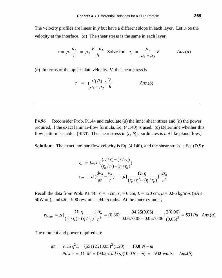
Chapter 4 Differential Relations for a Fluid Particle 369
The velocity profiles are linear in y but have a different slope in each layer. Let uI be the
velocity at the interface. (a) The shear stress is the same in each layer:
(b) In terms of the upper plate velocity, V, the shear stress is
________________________________________________________________________
P4.96 Reconsider Prob. P1.44 and calculate (a) the inner shear stress and (b) the power required, if the exact laminar-flow formula, Eq. (4.140) is used. (c) Determine whether this flow pattern is stable. [HINT: The shear stress in (r, ) coordinates is not like plane flow.] Solution: The exact laminar-flow velocity is Eq. (4.140), and the shear stress is Eq. (D.9):
Recall the data from Prob. P1.44: ri = 5 cm, ro = 6 cm, L = 120 cm, = 0.86 kg/m-s (SAE 50W oil), and i = 900 rev/min = 94.25 rad/s. At the inner cylinder,
The moment and power required are
).(forSolve21
221 aAnsVu
h
uV
h
uI
II
).()(21
21 bAnsh
V
2
( / ) ( / )[ ]( / ) ( / )
2( ) [ ]
( / ) ( / )
o oi i
o i i o
i i or
o i i o
r r r rv r
r r r r
dv v r r
dr r r r r r r
2 2
2 94.25(0.05) 2(0.06)[ ] (0.86)[ ] .( )( / ) ( / ) 0.06 / 0.05 0.05 / 0.06 (0.05)
i i o
innero i i o i
r rPa Ans a
r r r r r531
2 22 (531) 2 (0.05) (1.20)
(94.25 / )(10.0 ) .( )i i
i
M r L N m
Power M rad s N m watts Ans b
10.0
943
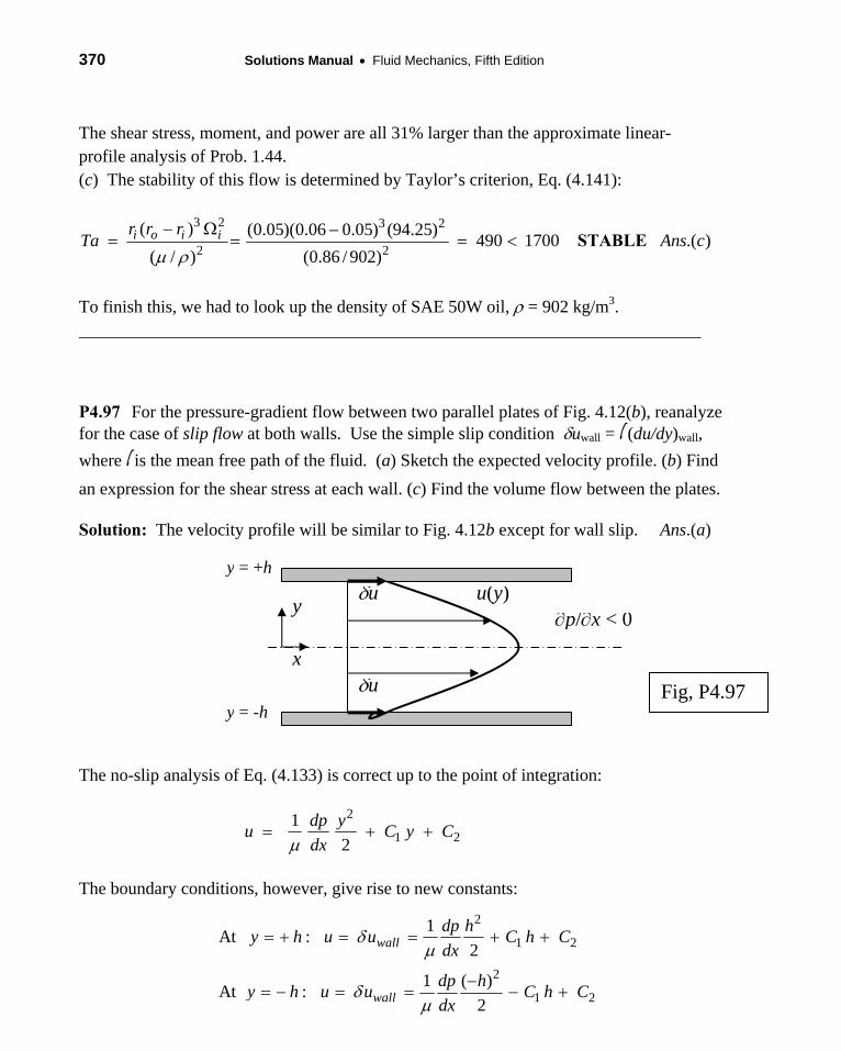
370 Solutions Manual Fluid Mechanics, Fifth Edition
The shear stress, moment, and power are all 31% larger than the approximate linear-profile analysis of Prob. 1.44. (c) The stability of this flow is determined by Taylor’s criterion, Eq. (4.141):
To finish this, we had to look up the density of SAE 50W oil, = 902 kg/m3. _______________________________________________________________________
P4.97 For the pressure-gradient flow between two parallel plates of Fig. 4.12(b), reanalyze for the case of slip flow at both walls. Use the simple slip condition uwall = l (du/dy)wall,
where l is the mean free path of the fluid. (a) Sketch the expected velocity profile. (b) Find
an expression for the shear stress at each wall. (c) Find the volume flow between the plates.
Solution: The velocity profile will be similar to Fig. 4.12b except for wall slip. Ans.(a)
The no-slip analysis of Eq. (4.133) is correct up to the point of integration:
The boundary conditions, however, give rise to new constants:
y
x
u(y)u
u
p/x < 0
Fig, P4.97
y = +h
y = -h
2
1 21
2
dp yu C y C
dx
2
1 2
2
1 2
1At :
2
1 ( )At :
2
wall
wall
dp hy h u u C h C
dx
dp hy h u u C h C
dx
3 2 3 2
2 2
( ) (0.05)(0.06 0.05) (94.25)490 1700 .( )
( / ) (0.86 / 902)i o i ir r r
Ta Ans c
STABLE
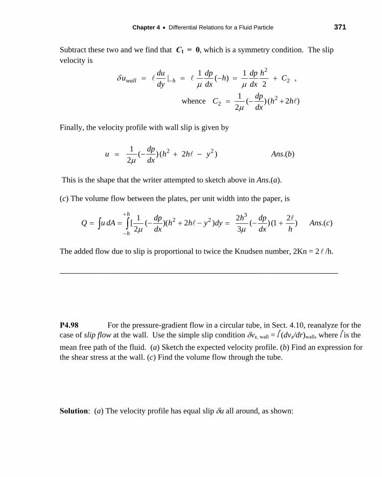
Chapter 4 Differential Relations for a Fluid Particle 371
Subtract these two and we find that C1 = 0, which is a symmetry condition. The slip velocity is
Finally, the velocity profile with wall slip is given by
This is the shape that the writer attempted to sketch above in Ans.(a).
(c) The volume flow between the plates, per unit width into the paper, is
The added flow due to slip is proportional to twice the Knudsen number, 2Kn = 2 /h.
______________________________________________________________________
P4.98 For the pressure-gradient flow in a circular tube, in Sect. 4.10, reanalyze for the case of slip flow at the wall. Use the simple slip condition vz, wall = l (dvz/dr)wall, where l is the
mean free path of the fluid. (a) Sketch the expected velocity profile. (b) Find an expression for the shear stress at the wall. (c) Find the volume flow through the tube.
Solution: (a) The velocity profile has equal slip u all around, as shown:
2
2
22
1 1| ( ) ,
2
1whence ( ) ( 2 )
2
wall hdu dp dp h
u h Cdy dx dx
dpC h h
dx
2 21( ) ( 2 ) .( )
2
dpu h h y Ans b
dx
32 21 2 2
[ ( )( 2 ) ( ) (1 ) .( )2 3
h
h
dp h dpQ u dA h h y dy Ans c
dx dx h
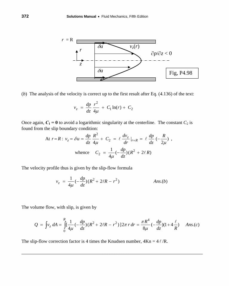
372 Solutions Manual Fluid Mechanics, Fifth Edition
(b) The analysis of the velocity is correct up to the first result after Eq. (4.136) of the text:
Once again, C1 = 0 to avoid a logarithmic singularity at the centerline. The constant C2 is found from the slip boundary condition:
The velocity profile thus is given by the slip-flow formula
The volume flow, with slip, is given by
The slip-flow correction factor is 4 times the Knudsen number, 4Kn = 4 /R.
____________________________________________________________________________
r
z
vz(r)u
u
p/z < 0
Fig, P4.98
r = R
2
1 2ln( )4z
dp rv C r C
dz
2
2
22
At : | ( ) ,4 2
1whence ( ) ( 2 )
4
zz r R
dvdp R dp Rr R v u C
dz dr dz
dpC R R
dz
2 21( ) ( 2 ) .( )
4zdp
v R R r Ans bdz
42 2
0
1[ ( ) ( 2 ) ]2 ( )(1 4 ) .( )4 8
R
zdp R dp
Q v dA R R r r dr Ans cdz dz R
Chapter 4 Differential Relations for a Fluid Particle 373
FUNDAMENTALS OF ENGINEERING EXAM PROBLEMS: Answers
Chapter 4 is not a favorite of the people who prepare the FE Exam. Probably not a single
problem from this chapter will appear on the exam, but if some did, they might be like these:
FE4.1 Given the steady, incompressible velocity distribution V 3xi Cyj 0k,
where C is a constant, if conservation of mass is satisfied, the value of C should be
(a) 3 (b) 3/2 (c) 0 (d) –3/2 (e) –3
FE4.2 Given the steady velocity distribution V 3xi 0j Cyk, where C is a constant,
if the flow is irrotational, the value of C should be
(a) 3 (b) 3/2 (c) 0 (d) –3/2 (e) –3
FE4.3 Given the steady, incompressible velocity distribution V 3xi Cyj 0k,
where C is a constant, the shear stress xx at the point (x, y, z) is given by
(a) 3 (b) (3x Cy) (c) 0 (d) C (e) (3 C)
FE4.4 Given the steady incompressible velocity distribution u = Ax, v = By, and w = Cxy, where (A, B, C) are constants. This flow satisfies the equation of continuity if A equals
(a) B , (b) B + C , (c) B – C , (d) – B , (e) –(B + C) FE4.5 For the velocity field in Prob. FE4.4, the convective acceleration in the x direction is
(a) A x2 , (b) A2 x , (c) B2 y , (d) B y2 , (e) C x2 y
FE4.6 If, for laminar flow in a smooth straight tube, the tube diameter and length both double, while everything else remains the same, the volume flow rate will increase by a factor of
(a) 2 , (b) 4 , (c) 8 , (d) 12 , (e) 16
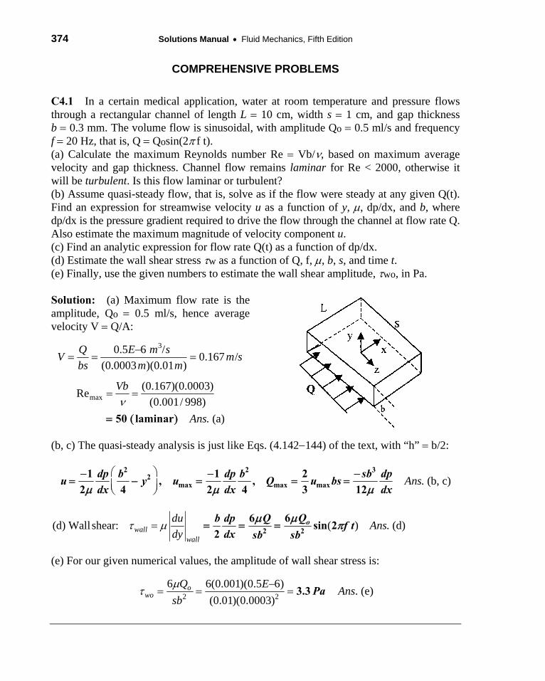
374 Solutions Manual Fluid Mechanics, Fifth Edition
COMPREHENSIVE PROBLEMS
C4.1 In a certain medical application, water at room temperature and pressure flows through a rectangular channel of length L 10 cm, width s 1 cm, and gap thickness b 0.3 mm. The volume flow is sinusoidal, with amplitude Qo 0.5 ml/s and frequency f 20 Hz, that is, Q Qosin(2 f t). (a) Calculate the maximum Reynolds number Re Vb/, based on maximum average velocity and gap thickness. Channel flow remains laminar for Re < 2000, otherwise it will be turbulent. Is this flow laminar or turbulent? (b) Assume quasi-steady flow, that is, solve as if the flow were steady at any given Q(t). Find an expression for streamwise velocity u as a function of y, , dp/dx, and b, where dp/dx is the pressure gradient required to drive the flow through the channel at flow rate Q. Also estimate the maximum magnitude of velocity component u. (c) Find an analytic expression for flow rate Q(t) as a function of dp/dx. (d) Estimate the wall shear stress w as a function of Q, f, , b, s, and time t. (e) Finally, use the given numbers to estimate the wall shear amplitude, wo, in Pa.
Solution: (a) Maximum flow rate is the amplitude, Qo 0.5 ml/s, hence average velocity V Q/A:
30.5 6 /0.167 /
(0.0003 )(0.01 )
Q E m sV m s
bs m m
max(0.167)(0.0003)
Re(0.001/ 998)
. (a)
Vb
Ans
50 laminar
(b, c) The quasi-steady analysis is just like Eqs. (4.142144) of the text, with “h” b/2:
. (b, c)Ans
dp b dp b sb dpu y u Q u bs
dx dx dx
2 2 32
max max max1 1 2
, ,2 4 2 4 3 12
(d) Wall shear: ( ) . (d)wallwall
duAns
dy oQb dp Q
f tdx sb sb2 2
66sin 2
2
(e) For our given numerical values, the amplitude of wall shear stress is:
2 2
6 6(0.001)(0.5 6)
(0.01)(0.0003)o
woQ E
sb
3.3 Pa Ans. (e)
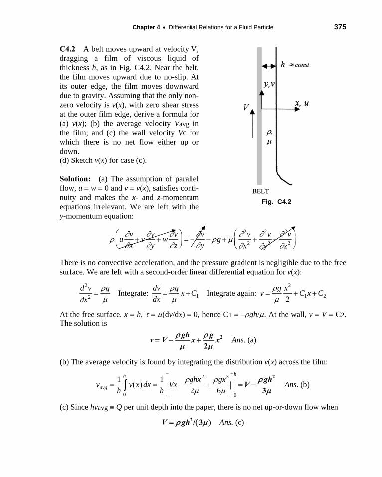
Chapter 4 Differential Relations for a Fluid Particle 375
C4.2 A belt moves upward at velocity V, dragging a film of viscous liquid of thickness h, as in Fig. C4.2. Near the belt, the film moves upward due to no-slip. At its outer edge, the film moves downward due to gravity. Assuming that the only non-zero velocity is v(x), with zero shear stress at the outer film edge, derive a formula for (a) v(x); (b) the average velocity Vavg in the film; and (c) the wall velocity VC for which there is no net flow either up or down. (d) Sketch v(x) for case (c).
Solution: (a) The assumption of parallel flow, u w 0 and v v(x), satisfies conti-nuity and makes the x- and z-momentum equations irrelevant. We are left with the y-momentum equation:
Fig. C4.2
2 2 2
2 2 2
v v v v v v vu v w g
x y z y x y z
There is no convective acceleration, and the pressure gradient is negligible due to the free surface. We are left with a second-order linear differential equation for v(x):
2 2
1 1 22Integrate: Integrate again:
2
d v g dv g g xx C v C x C
dxdx
At the free surface, x h, (dv/dx) 0, hence C1 –gh/. At the wall, v V C2. The solution is
. (a)Ansgh g
v V x x
2
2
(b) The average velocity is found by integrating the distribution v(x) across the film:
2 3
0 0
1 1( ) . (b)
2 6
hh
avgghx gx
v v x dx Vx Ansh h
ghV
2
3
(c) Since hvavg Q per unit depth into the paper, there is no net up-or-down flow when
. (c)AnsV gh 2 / 3
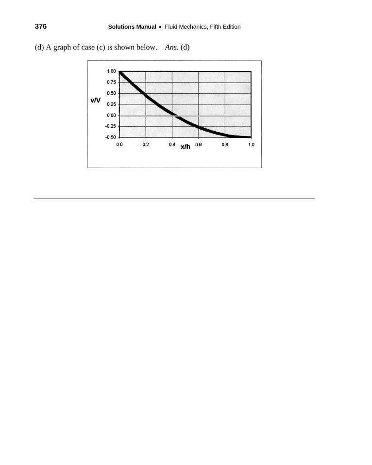
376 Solutions Manual Fluid Mechanics, Fifth Edition
(d) A graph of case (c) is shown below. Ans. (d)