Photogrammetry for Dimensional Control of Bridges

by

S. A. Veress University of Washington

Department of Civil Engineering Seattle, Wa 98195

USA

ABSTRACT

A curved segmental concrete bridge at Vail Pass, Colorado was the sub­ject of investigation. The geometric property of the nrecast segments were determined by analytical photogrammetry. This data was compared to design data to obtain quality control for casting . The segments, as determined by photogrannnetry, were connected mathematically to obtain a "dry fit". The "dry fit" compared to the actual fit provided data for constructional qual­ity control . The mathematical solutions for field control and photogramme­try are discussed along with the error propagation of the "dry fit" .

1 . Introduction

The modern precast segmental bridge design provides an opportunity for further expansion of an application of photogrammetry . Such a photogrammet­ric application is utilized in the case of Vail Pass ' curved segmental con­crete bridge . Photogrammetric studies were conducted on the precast elements. These studies permit dimensional analysis of each element for comparison of achieved dimensions and deviations from designed dimensions and detects dis­tortions due to casting and/or storage process . This enables a cantilever to be mathematically "dry fit" to predict erected geometry with " zero" joint widths .

2. Control Survey

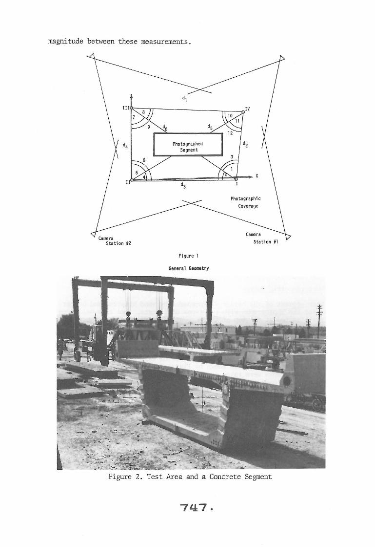
A test area was developed by a control survey where 26 segments of the curved concrete bridge was photogrammetrically surveyed. The geometry of the test area is shown by Figure 1, where the ground control points are designated as I, II, III and IV measured angles numbered from 1 to 12 and measured distances are shown as d , d2, ,, d6 .

The control points consist ot 2 1nch lll diameter steel pipe driven into the ground approximately one meter until zero penetration . The top of the pipe is fitted with a ceramic ball of 32 . 13 ±0.13 rnm for a reference point . The overall view of the test area is shown by Figure 2. The concrete bridge segments were placed by a Travel Lift onto the center of the control net for a premarked position. A horizontal control survey was established by distance and angle measurements . Distances were measured with invar tape and the angles were measured by a theodolite with a least-reading of one second . The maximum discrepancy was found to be 13 .1 and the minimum -0 . 4 of a second of arch.

The horizontal control net was adjusted by trilateration ; the angle measurement was used only for control . The elevations obtained by a Kern leveling instrument equipped with an optical micrometer . The leveling was performed in the morning and in the eveni ng before and after photography . The repeated measurements were only precautions against a possible motion due to the Travel Lift Movement, there was no difference of respectable

7LJ:S.

magnitude between these measurements .

Photographed Segment

Figure 1

General Geometry

Photographic Coverage

Camera Station Ill

Figure 2. Test Area and a Concrete Segment

7/47.

1ne coordinates of station II were selected as X = 100 . 00 m, Y = 100.00 m. The orientation of the ground coordinates system was such that the Y axis coincides with II - III line .

The general function for the least-squares adjustment to obtain the ground coordinates is:

X.)2 + (Y . - Y.)2 = F(X., Y., X. , Y.) ...........•.. (2.1) l J l l J J J

where d .. is the measured distance between J and I net points (the measured distanceJranged from d4 = 6.514 m to d5 = 12.464 m).

Approximate coordinates (XQ, Y0 ) were introduced for the net points and linearized by the Taylor Series to form an observation equation for the least-squares adjustment, which in a general form is:

v . . i£__ !::.X. + i£__ 'Y + iL_ 'X. + aF 'Y [d F(X Y X Y )] lJ ax

0. J aY

0. Ll j aX

0. Ll 1 aY

0. Ll j - ij + i' i' j ' j

J J l J or

V- 1'0(- L· ....................................................... (2.2)

Where the X matrix is composed of X's andY's and is computed from the nor-mal equation by: x = (ATAfl ATL ...................................... (2.3) The probable coordinate values and their standard errors are:

X. = X + !':.X. , Y . = Y + !:::. Y . . aX2 l o. l l o . l

l l

002 ()XX ' (J 2 = v Tv ................. ( 2 . 4) o n-u

The maximum and minimum values for t he connuted standard errors are :

±0.92 mrn.

3. Photogra..rnmetric Survey

Each ser.ment of the bridge was prepared by sand blasting and by tar­geting for t 1-:e photographs with two types of targets. One is a ball type of target located at the top of the segments (see Figure 2. ). These targets were leve:ecl nreviou.s to the photographs. Two is the painted targets, which are locate .~ at the match cast and bulkhead end of the segments. Stencils were made for the painted targets which matched the shape of the segments, thus, the targets (1-1/2" in diameter dots) were placed near (within 1 mm) the same part of each segment. The total of 68 targets were placed on each segment and their location is shown by Figure 2 and 4.

The photographs were taken from about 15 m photographic distance. Hasselblad MK 70 cameras with f = 60 mm were used. Four photographs were made from each segment and 26 segments were photographed.

The photographs were measured on the analytical plotter at the Univer­sity of 1Vashington. The photo-coordinates were obtained from the negative and their average standard error was ±3 micrometers .

The photogrammetric data reduction consisted of the following steps. 1) Space resection. 2) Determination of the orientation matrix. 3) Space intersection.

The geometrical princinle of these steps is shown by Figure 3. and described as follows: The machine coordinates are obtained by the analyti­cal plotter and transformed into the photo-coordinate system, using the known coordinates of the reseau, b)' affine transformation. The approximate coordinates X , Y , Z of the camera station for the space resection were

0 0 0

7l:I:B.

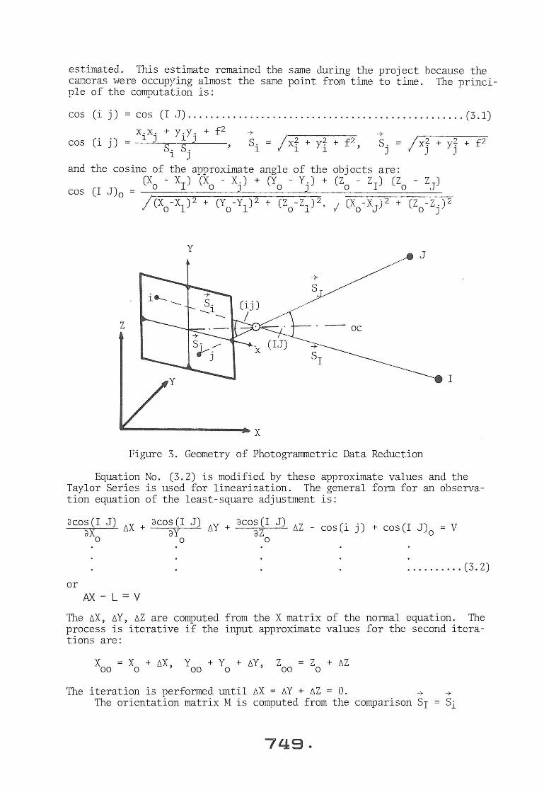
estimated. This estimate remained the same during the project because the cameras were occup.ring almost the same point from time to time. The princi­ple of the computation is:

cos (i j) cos (I J) ................................................. (3 .1) x.x. + y .y . + f 2 -+ -+

cos (i j) l J l J s. s.

l J S. = /x? + y? + f 2 S.

l l l ' J /xj + Yj + f2

and the cosine of the approximate angle of the objects are: (X - X

1) (X - X.) + (Y - Y.) + (Z - ZI) (Z - ZJ)

cos (I J)o = o o J o J o o

l ex -x ) 2 + (Y -Y ) 2 + cz -z ) 2. 1 ex -x )2 + cz -z.)2 0 1 0 1 0 1 y 0 J 0 J

y -~ J

-+ s

z . -- oc

Figure 3. Geometry of Photogrammetric Data Reduction

Equation No . (3 . 2) is modified by these approximate values and the Taylor Series is used for linearization. The general form for an observa­tion equation of the least-square adjustment is:

acos(I J) ~X+ acos(I J) ~y + acos(I J) ~ Z _ cos(i J.) + cos(I J) = v ax aY az o

0 0 0

.......... (3. 2)

or

The ~X, ~Y, ~Z are computed from the X matrix of the normal equation. The process is iterative if the input approximate values for the second itera­tions are:

X = X + ~X, Y + Y + ~Y, Z 00 0 00 0 00

z + ~z 0

The iteration is performed until ~X = ~Y + ~Z = 0. -+ -+ The orientation matrix M is comDuted from the comparison SI = Si

7£:&:9.

vectors in Figure 3. The relationship between these two vectors is: + +

M' SI = s. 1

or in detail : mll' ml2' m13 cos XIO cos xiO

m21' m22' m23 cos YIO = cos yiO

m31' m32' m33 cos ZIO cos ziO .............. (3 . 3)

where the direction cosines were computed from the vector components . Be­cause theM orientation matrix has nine terms in it, the minimum of three points are required to solve M. That is:

+ + + + + + -1 M = (Si · Sj · Sk) (SI · SJ · SK) .............................. (3 . 4)

The least-squares adjustment must be used to solve the term in M matrix if four control points are given such as in this project.

The spatial coordinates of the targets are determined by space inter­section, from which equations of the line to the target I from camera sta­tions 1 and 2 are :

z - z I 01

cos zo1r

YI - YO 2I - 20 2 2

--.rr;:-.,.,- = ----,~..., cos Y02I oos zo2I ................................... (3 . 5)

The targets located on the side of the segment were visible and photo­graphed from two cam~ra stations and the targets located on the top of the segment was photographed from four camera stations . Thus, for each target two or four equations such as No . (3 . 5) were written and a least-squares adjustment was used to obtain the X, Y, Z coordinates of each target . The average standard error of the coordinates were found to be ±1 . 1 mrn .

The final product of the photogramrnetric survey, therefore, is the co­ordinates of the target in the system of ground control which will be called ''Ground Coordinates'' .

4. Geometrical Control of Concrete Segments

The ground coordinates of the targets of the segments changed. The numerical value of the corresponding targets varied from segment to segment depending upon how the Travel Lift placed the segments into the premarked position for photography . This variation in the coordinates made the deter­mination of the proper geometrical shape of each segment difficult . There­fore, a local coordinate system has been chosen whose axes are located on each segment, and from these coordinates the physical dimension of the segment is readily obtainable .

In the local coordinate system, the X axis is located at the base of the concrete segment on the bulkhead side , the Y axis is perpendicular to it at the ·center line of the segment at its base and the Z is perpendicular to the X Y plane . The arrangement of this local coordinate system is shown

750.

by Figure 4.

z

Figure

Formula (4 . 1) was used coordinates .

XL mll' ml2'

56- 58 Targets

X Local Coordinate System

4. Local Coordinate System

for the transformation from ground to

ml3 XG T X

local

YL = m21 ' m22' m23 + YG + T ................ (4 . 1) y

ZL m31' m32 ' m33 ZG T z -

The G and L subscripts indicate ground and local coordinates, the m's deter­mine the rotational matrix and the Tx, Ty, Tz are the translational elements in X, Y, Z direction . First, four points were chosen whose coordinates were computed in both systems and these were used to determine the rotational matrix and the translational elements . Then the transformation of all the coordinates was nerformed.

The local coordinates were then compared to the des i gn dimension of the segment for a quality check . Further, the geometry of cast and match faces were drawn according to the local coordinates . A sample of such a drawing is represented by Figure 5. for segments V2W-5, V2W-6 and V2W-7 . This numerical and graphical documentation provides the bases for an evalu­ation of the major dimensions, web and slab thickness , geometry of the sides (I . E. exterior angles) and deviations of the end faces . Thus, a complete quality check of the casting yard has been provided .

5. Dry Fit for Construction Control

The mathematical "dry fit" consists of two parts :

1. To connect the individual section into a single unit in the ground coordinate system.

2. To use this assembled unit as a rigid body to transform it to the field coordinate system as given at the pier on section E- 2 and W-2 (Figure 5. ) .

Individual connections of the sections were performed in the ground co­ordinate system using the target on the corresponding side of the segments . The transformations were performed by the same equation as equation No . (4 . 1).

75:1..

The details of this computation provided the orientation matrices and the coordinates of each target with their standard errors in the ground coordi­nate system of the first segment .

17-1

31

62-32

. 007 m1- ····· 66-36 f"" .

targets 1 1

I

:; .005] 83-33

87-57

V2W-7

62-32

I I . 008 mr··· 66-36 r· .. 009 m

.007 m 1 I

I

. . 002 m~ 83-33 -.002 m

87-57

V2W-6 V2W-5

Figure 5. Geometry of Cast and Match Cast Faces

\ '2W 3 - V2W 2 - <

28-1 88 58 88

l2s -- 0 0 -- 0 0 0 0

26 25 26 Pie 24 23 24

Segme t XF 1000 m

y"C 1000 m ZF

. ZF 1000 P.1

23 24 23 24 26 25 26 0 0 0 0 0 0 0

88 58 88 -- --

16-28 V2E-2 V2E-3

Figure 6. Field Coordinate System

5 8 0

23

25 0

The second computation was performed to fit the unified segments into the Field Coordinate System. These coordinates served as a check upon con­struction by comparing them with the design data.

The standard errors of the coordinates of the targets made it possible to compute the error propagation.

The general equation is used

U f(x y z) then 0 2 = (au)2

' ' u ax

for error propagation if the

02 + (au)202 + (au)2 02 x ay y az z

752.

function is:

The error in the mathematical "dry fit" grow progressively as more and more segments are connected. The errors were computed along both edges (webs) of the segments which are the most critical lines. The illustration of the accumulated errors are shown by Figure 7. for one side of the bridge which clearly indicates that the most critical are the vertical and perpen­di~ular directions to the center line of the bridge.

±ax y or Z .rrnn . Error Propagation Along Points ' 32/62 (2)

30 Se

20

10 -0 W-2 W-3 W-4 W-5 W-6 W-7 V-8 1V-9 W-10 W-1

±ax '

y or Z mm. Error Propagation Along Points

30 57/87 (27) Segments

20

10

0 iv.:.-z w..:3 1\T-4 W-5 W-6 W-7 'W-8

Figure 7. Error Propagation

The error in the mathematical "dry fit" grow progressively as more and more segments are connected. The errors were computed along both edges (webs) of the segments which are the most critical lines. The illustration of the accumulated errors are shown by Figure 7. for one side of the bridge which clearly indicates that the most critical are the vertical and per­pendicular directions to the center line of the bridge.

6. Discussion

This project of industrial application of photogrammetry indicates that one of the most influential factors on achievable accuracy is the precision of a control net . The preparation of the concrete segments by sand blasting is completely adequate in providing a reasonably smooth surface for the photogrammetric survey.

The overall precision of the photograrnmetric survey was adequate as far as the determination of the major dimensions of the segments. A qual­ity control was provided not only for the casting but for the storage. Qualit)' control was also provided, particularly because the deck slab be­tween the webs had a tendency to shrink away from the bulkhead due to the lack of restraints. The maximum value of this deviation is 13.1 mm. The mathematical "dry fit" of the elements to compare the resulting assembled cantilever with the casting curves was less successful then hoped for. It was concluded that propagated errors were of the same order of magnitude as the physical discrepancies which could produce observable displacements from the casting curves.

753.

Acknowledgement

This project was performed for the Colorado State Department of High­ways through Arvid Grant and Associ ates, Inc . The author would like to ex­press his gratitude to Dr . M. C. Y. Hou of the University of Washington for his contribution.

Selected References

1. American Society of Photogrammetry, Handbook of Non-Topographic Photo­grammetry, 1979 .

2. Brandenberger, A. J . and Erez, M. T. , "Photogrammetric Determination of Deformations in Large Engineering Structures", Canadian Surveying, Vol . 26 , Nov . 2, 1972 .

3. Cotovanu , E, "Messung von Brucken durch terrestrische Photogrammetrie", Buletin de Fotogrammetrie , Special Issue, 1972 .

4. Erez , M. T., "Analytical Terrestrial Photogrammetry Applied to the Heasurement of Deformations in Large Engineering Structures , 1 1 Disserta­tion, University of Laval, 1971 .

5. Erlandson, J . P. and Veress , S. A. , "Contemporary Problems in Terrestri­al Photogrammetry , " Photogramtnetric Engineering , Vol. XL, pp 1079-1085, 1974 .

6. Erlandson, J . P. and Veress, S. A. , "Photogral!IDletrische Erfassung von Bauwerksveranderungen," VR-Vermessungswesen und Raumordnung, Vol . 8, 1976 .

7. Planick , A., "Die Benutzung der terrestrischen Photogrammetrie in De­formationsmessung von Steinschuttendammen," Paper presented at the 6th International Meeting on High Precision Engi neering Surveys , 1970 .

8. Veress, S. A., "Adjustment by Least-Squares ," American Congress on Surveying and Mapping , 1974 .

9. Veress, S. A. , "Determination of Motion and Deflection of Retaining Walls" , Part I and IIfmTheoretical Considerations, University of Washington , Final Tee ical Report , 1971 .