Embed Size (px)
Citation preview
88
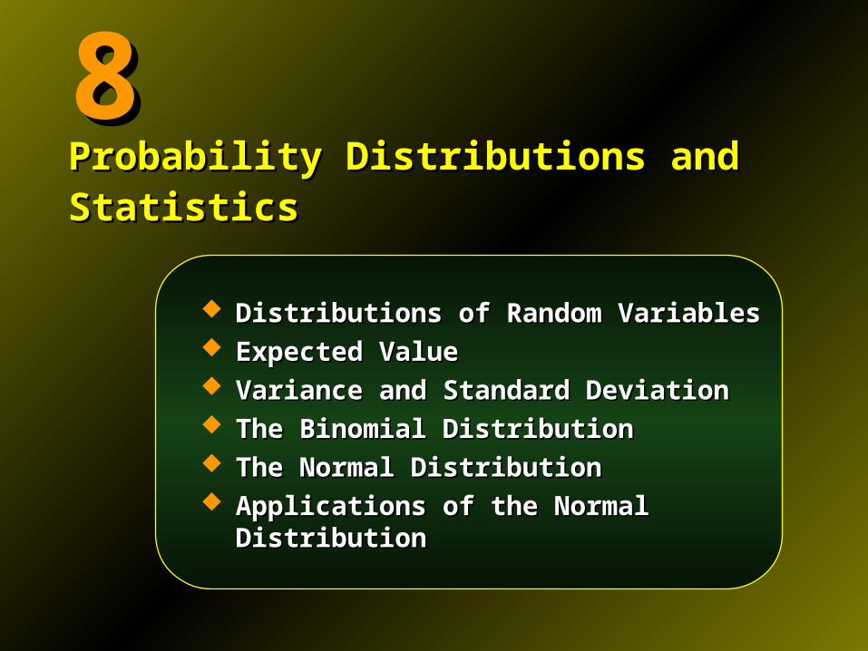
Distributions of Random VariablesDistributions of Random Variables Expected ValueExpected Value Variance and Standard DeviationVariance and Standard Deviation The Binomial DistributionThe Binomial Distribution The Normal DistributionThe Normal Distribution Applications of the Normal DistributionApplications of the Normal Distribution
Probability Distributions and StatisticsProbability Distributions and Statistics
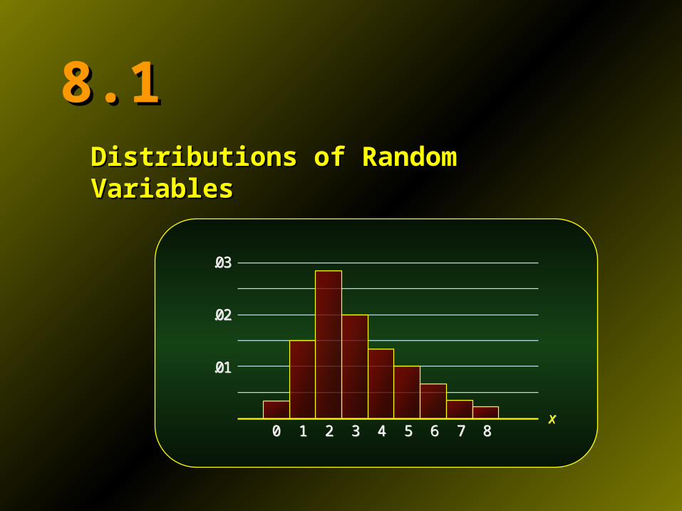
8.18.1Distributions of Random VariablesDistributions of Random Variables
00 11 22 33 44 55 66 77 88
.03.03
.02.02
.01.01
xx

Random VariableRandom Variable
A random variable is a rule that assigns A random variable is a rule that assigns a number to each outcome of a chance a number to each outcome of a chance experiment.experiment.
ExampleExample
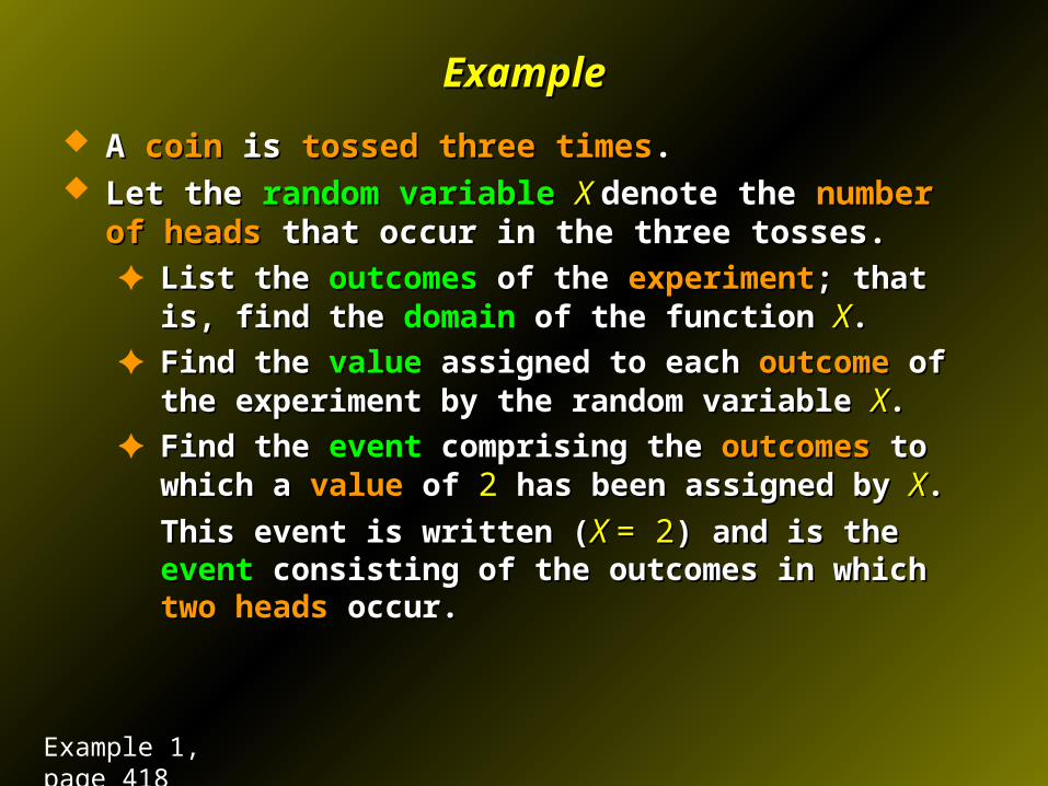
A A coincoin is is tossed three timestossed three times. . Let the Let the random variablerandom variable X X denote the denote the number of headsnumber of heads
that occur in the three tosses.that occur in the three tosses.✦ List the List the outcomesoutcomes of the of the experimentexperiment; that is, find the ; that is, find the
domaindomain of the function of the function XX..
✦ Find the Find the valuevalue assigned to each assigned to each outcomeoutcome of the of the experiment by the random variable experiment by the random variable XX..
✦ Find the Find the eventevent comprising the comprising the outcomesoutcomes to which a to which a valuevalue of of 22 has been assigned by has been assigned by XX. .
This event is written (This event is written (X X = 2= 2) and is the ) and is the eventevent consisting of consisting of the outcomes in which the outcomes in which two headstwo heads occur. occur.
Example 1, page 418
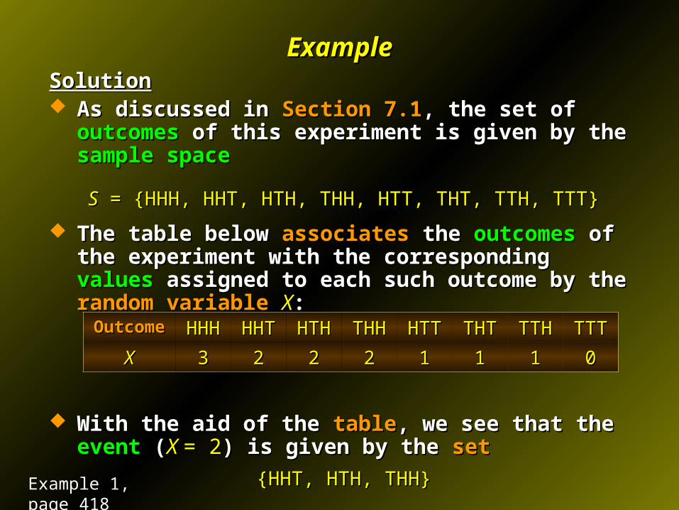
ExampleExampleSolutionSolution As discussed in As discussed in Section 7.1Section 7.1, the set of , the set of outcomesoutcomes of this of this
experiment is given by the experiment is given by the sample spacesample space
SS = {HHH, HHT, HTH, THH, HTT, THT, TTH, TTT} = {HHH, HHT, HTH, THH, HTT, THT, TTH, TTT}
The table below The table below associatesassociates the the outcomesoutcomes of the of the experiment with the corresponding experiment with the corresponding valuesvalues assigned to assigned to each such outcome by the each such outcome by the random variablerandom variable XX::
With the aid of the With the aid of the tabletable, we see that the , we see that the eventevent ( (X X = 2= 2) is ) is given by the given by the setset
{HHT, HTH, THH}{HHT, HTH, THH}
OutcomeOutcome HHHHHH HHTHHT HTHHTH THHTHH HTTHTT THTTHT TTHTTH TTTTTT
XX 33 22 22 22 11 11 11 00
Example 1, page 418
Applied Example: Applied Example: Product ReliabilityProduct Reliability
A disposable flashlight is turned on until its battery A disposable flashlight is turned on until its battery runs out.runs out.
Let the Let the random variablerandom variable Z Z denote the length (in hours) denote the length (in hours) of the of the lifelife of the battery. of the battery.
What What valuesvalues can can ZZ assume? assume?SolutionSolution The The valuesvalues assumed by assumed by ZZ can be any can be any nonnegativenonnegative real real
numbersnumbers; that is, the ; that is, the possible valuespossible values of of ZZ comprise the comprise the interval interval 0 0 ZZ < < ∞∞..
Applied Example 3, page 419
Probability Distributions and Random VariablesProbability Distributions and Random Variables
Since the Since the random variablerandom variable associated with an associated with an experimentexperiment is related to the is related to the outcomeoutcome of the experiment, of the experiment, we can construct a we can construct a probability distributionprobability distribution associated associated with the with the random variablerandom variable, rather than one associated , rather than one associated with the with the outcomes of the experimentoutcomes of the experiment..
In the next several examples, we illustrate the In the next several examples, we illustrate the construction of probability distributions.construction of probability distributions.
4
3( 4) ( )
36P X P E 4
3( 4) ( )
36P X P E
ExampleExample
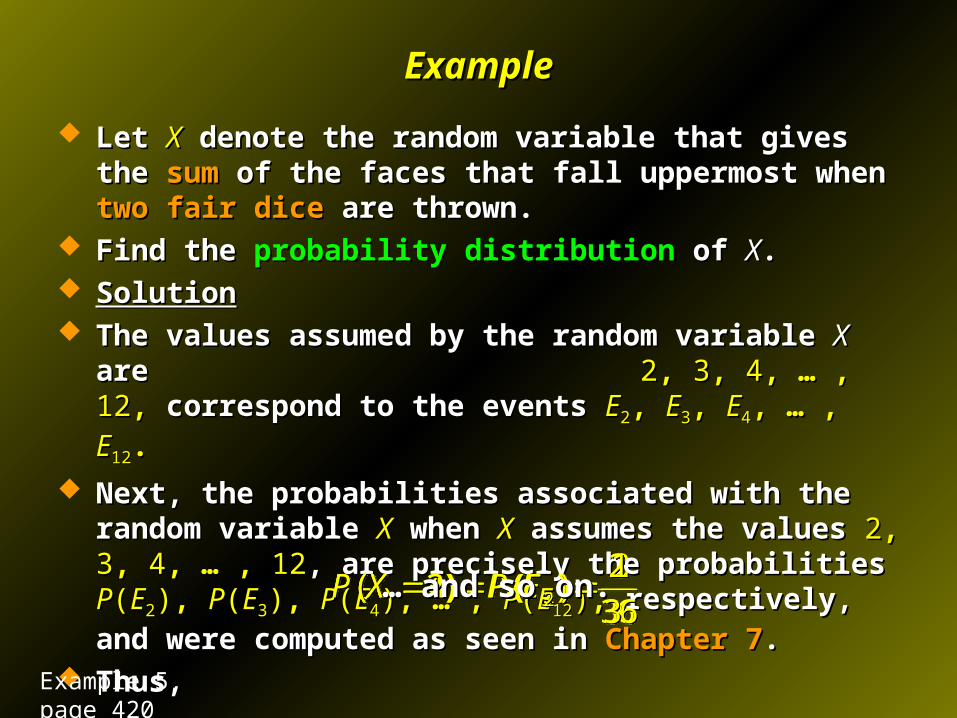
Let Let XX denote the random variable that gives the denote the random variable that gives the sumsum of the of the faces that fall uppermost when faces that fall uppermost when two fair dicetwo fair dice are thrown. are thrown.
Find the Find the probability distributionprobability distribution of of XX.. SolutionSolution The values assumed by the random variable The values assumed by the random variable XX are are
22, , 33, , 44, … , , … , 1212,, correspond to the events correspond to the events EE22, , EE33, , EE44, … , …
, , EE1212..
Next, the probabilities associated with the random Next, the probabilities associated with the random variable variable XX when when XX assumes the values assumes the values 22, , 33, , 44, … , , … , 1212, are , are precisely the probabilities precisely the probabilities PP((EE22)), , PP((EE33)), , PP((EE44)), … , , … , PP((EE1212)),,
respectively, and were computed as seen in respectively, and were computed as seen in Chapter 7Chapter 7.. Thus, Thus,
3
2( 3) ( )
36P X P E 3
2( 3) ( )
36P X P E 2
1( 2) ( )
36P X P E 2
1( 2) ( )
36P X P E … … and so on.and so on.
Example 5, page 420
Applied Example: Applied Example: Waiting LinesWaiting Lines
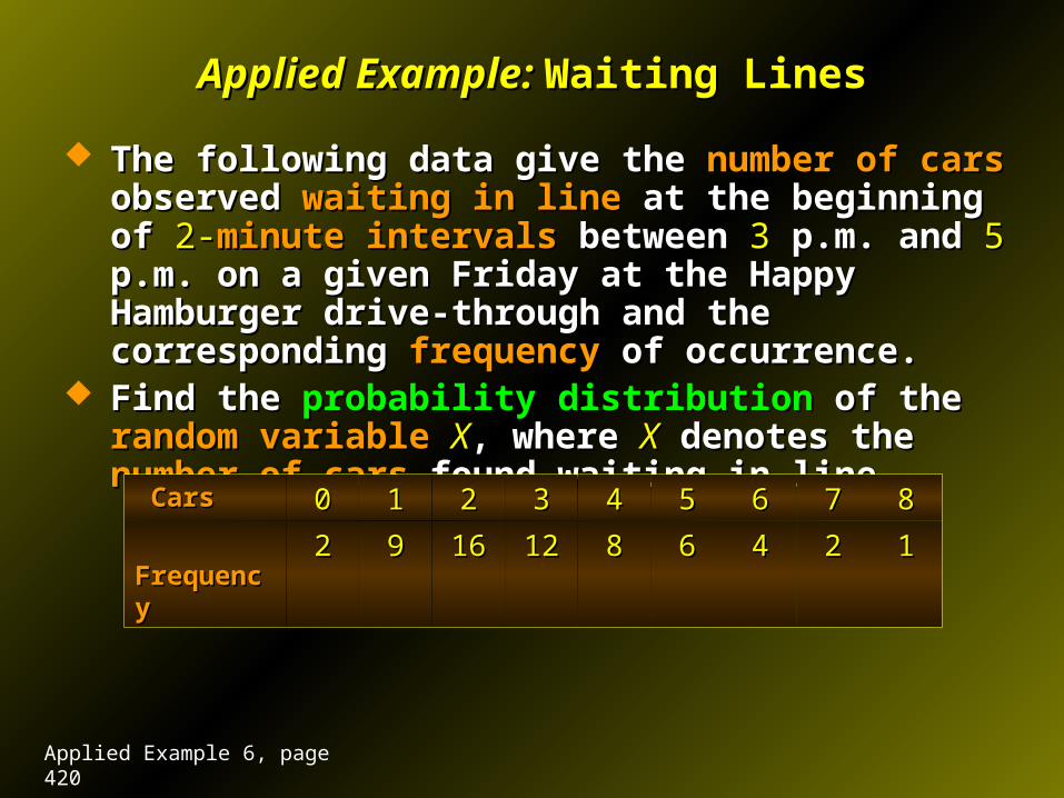
The following data give the The following data give the number of carsnumber of cars observed observed waiting in linewaiting in line at the beginning of at the beginning of 2-2-minute intervalsminute intervals between between 33 p.m. and p.m. and 55 p.m. on a given Friday at the Happy p.m. on a given Friday at the Happy Hamburger drive-through and the corresponding Hamburger drive-through and the corresponding frequencyfrequency of occurrence. of occurrence.
Find the Find the probability distributionprobability distribution of the of the random variablerandom variable XX, , where where XX denotes the denotes the number of carsnumber of cars found waiting in line. found waiting in line.
CarsCars 00 11 22 33 44 55 66 77 88
FrequencyFrequency 22 99 1616 1212 88 66 44 22 11
Applied Example 6, page 420
Applied Example: Applied Example: Waiting LinesWaiting Lines
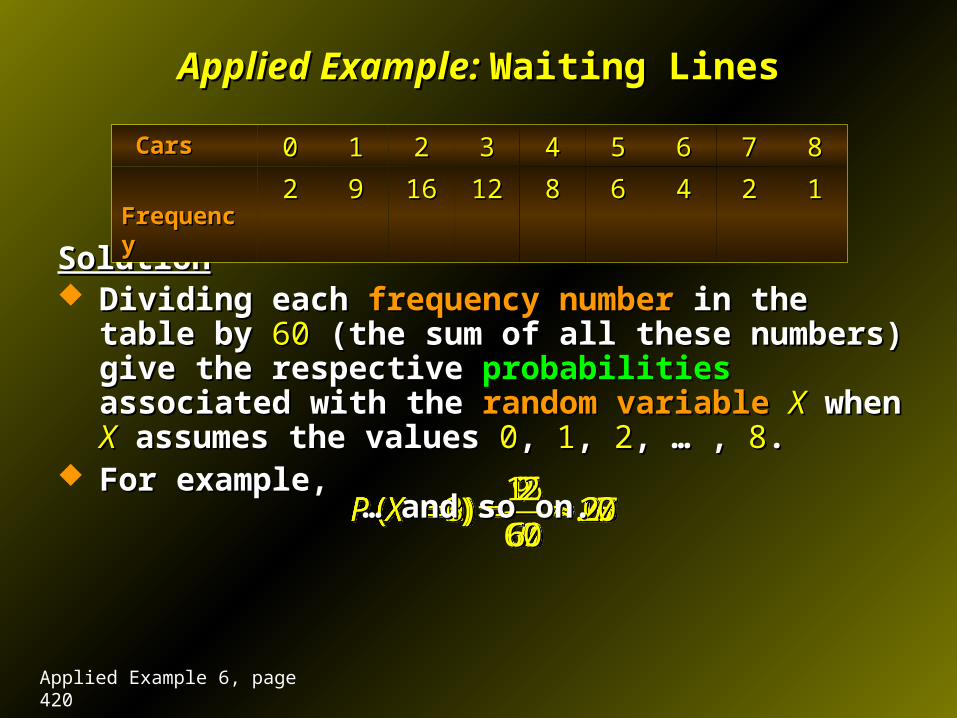
SolutionSolution Dividing each Dividing each frequency numberfrequency number in the table by in the table by 6060 (the (the
sum of all these numbers) give the respective sum of all these numbers) give the respective probabilitiesprobabilities associated with the associated with the random variablerandom variable XX when when XX assumes the assumes the values values 00, , 11, , 22, … , , … , 88..
For example,For example,
CarsCars 00 11 22 33 44 55 66 77 88
FrequencyFrequency 22 99 1616 1212 88 66 44 22 11
Applied Example 6, page 420
16( 2) .27
60P X
16( 2) .27
60P X 9
( 1) .1560
P X 9
( 1) .1560
P X 2( 0) .03
60P X
2( 0) .03
60P X 12
( 3) .2060
P X 12
( 3) .2060
P X … … and so on.and so on.
Applied Example: Applied Example: Waiting LinesWaiting Lines
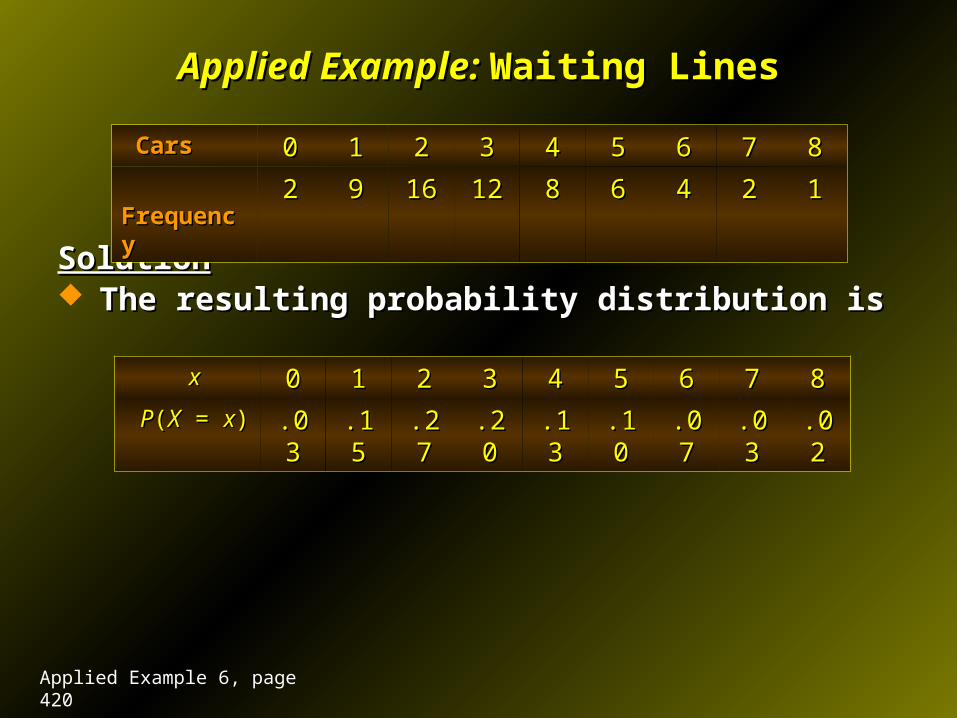
SolutionSolution The resulting probability distribution is The resulting probability distribution is
CarsCars 00 11 22 33 44 55 66 77 88
FrequencyFrequency 22 99 1616 1212 88 66 44 22 11
xx 00 11 22 33 44 55 66 77 88
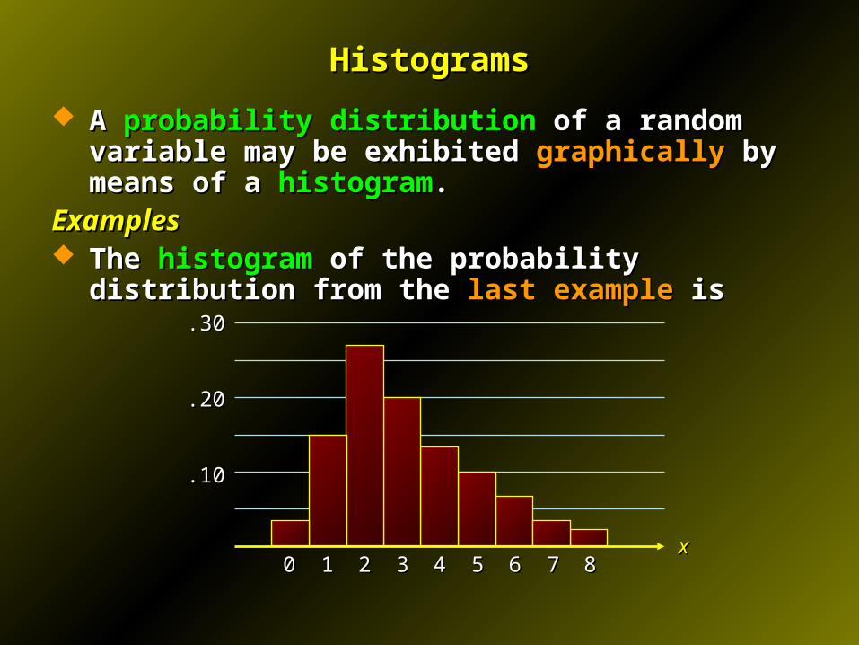
PP((XX = = xx)) .03.03 .15.15 .27.27 .20.20 .13.13 .10.10 .07.07 .03.03 .02.02
Applied Example 6, page 420
HistogramsHistograms
A A probability distributionprobability distribution of a random variable may be of a random variable may be exhibited exhibited graphicallygraphically by means of a by means of a histogramhistogram..
ExamplesExamples The The histogramhistogram of the probability distribution from the of the probability distribution from the last last
exampleexample is is
00 11 22 33 44 55 66 77 88
.30.30
.20.20
.10.10
xx
HistogramsHistograms
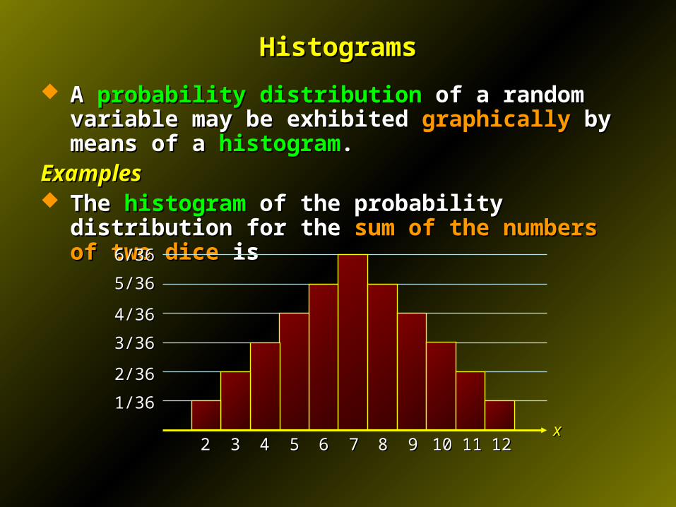
A A probability distributionprobability distribution of a random variable may be of a random variable may be exhibited exhibited graphicallygraphically by means of a by means of a histogramhistogram..
ExamplesExamples The The histogramhistogram of the probability distribution for the of the probability distribution for the sum sum
of the numbers of two diceof the numbers of two dice is is
22 33 44 55 66 77 88 99 1010 1111 1212
6/366/36
5/365/36
4/364/36
3/363/36
2/362/36
1/361/36
xx
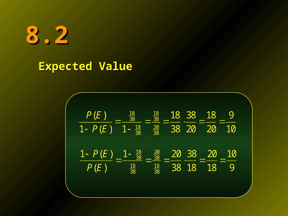
8.28.2Expected ValueExpected Value
18 2038 38
18 1838 38
1 ( ) 1 20 38 20 10
( ) 38 18 18 9
P E
P E
18 2038 38
18 1838 38
1 ( ) 1 20 38 20 10
( ) 38 18 18 9
P E
P E
18 1838 38
18 2038 38
( ) 18 38 18 9
1 ( ) 1 38 20 20 10
P E
P E
18 1838 38
18 2038 38
( ) 18 38 18 9
1 ( ) 1 38 20 20 10
P E
P E
Average, or MeanAverage, or Mean
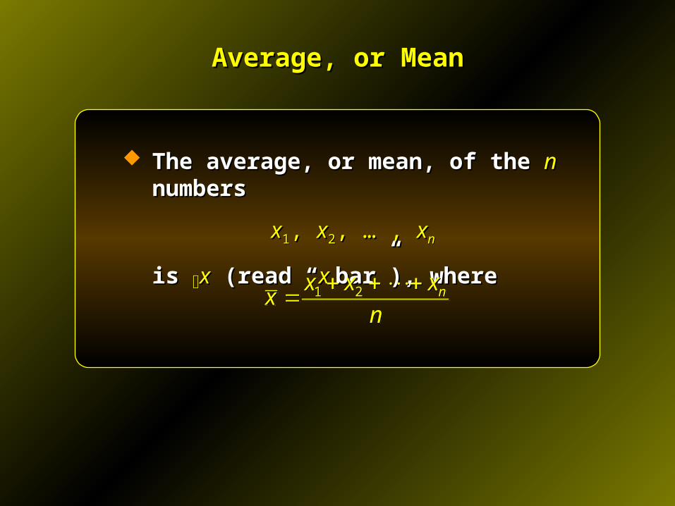
The average, or mean, of the The average, or mean, of the nn numbers numbers
xx11, , xx22, … , , … , xxnn
is is xx (read “ (read “x x bar”), wherebar”), where
1 2 nx x xx
n
1 2 nx x x
xn
Applied Example: Applied Example: Waiting LinesWaiting Lines
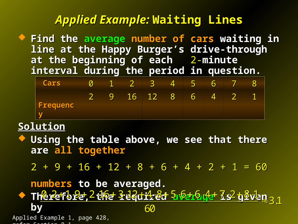
Find the Find the averageaverage number of cars number of cars waiting in line at the waiting in line at the Happy Burger’s drive-through at the beginning of each Happy Burger’s drive-through at the beginning of each 2-2-minute interval during the period in question.minute interval during the period in question.
SolutionSolution Using the table above, we see that there are Using the table above, we see that there are all togetherall together
2 + 9 + 16 + 12 + 8 + 6 + 4 + 2 + 1 = 602 + 9 + 16 + 12 + 8 + 6 + 4 + 2 + 1 = 60
numbersnumbers to be averaged. to be averaged. Therefore, the required Therefore, the required averageaverage is given by is given by
CarsCars 00 11 22 33 44 55 66 77 88
FrequencyFrequency 22 99 1616 1212 88 66 44 22 11
0 2 1 9 2 16 3 12 4 8 5 6 6 4 7 2 8 13.1
60
0 2 1 9 2 16 3 12 4 8 5 6 6 4 7 2 8 13.1
60
Applied Example 1, page 428, refer Section 8.1
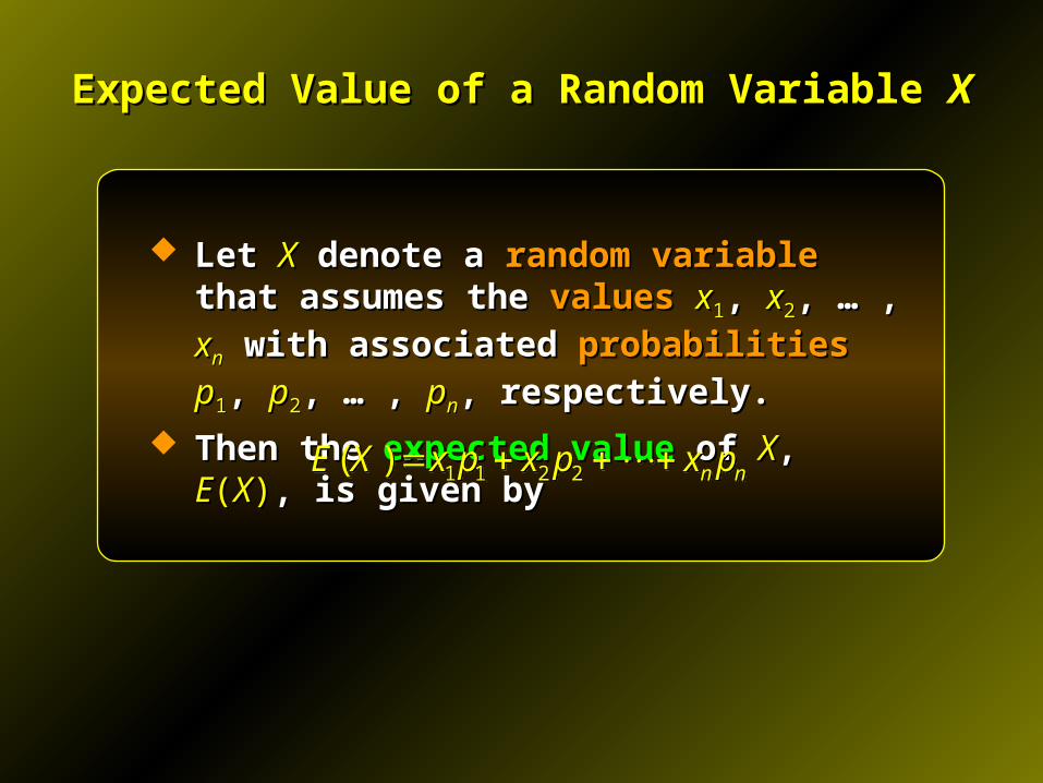
Expected Value of a Random Variable Expected Value of a Random Variable XX
Let Let XX denote a denote a random variablerandom variable that assumes that assumes the the valuesvalues xx11, , xx22, … , , … , xxnn with associated with associated
probabilitiesprobabilities pp11, , pp22, … , , … , ppnn, respectively., respectively.
Then the Then the expected valueexpected value of of XX, , EE((XX)), is given by, is given by
1 1 2 2( ) n nE X x p x p x p 1 1 2 2( ) n nE X x p x p x p
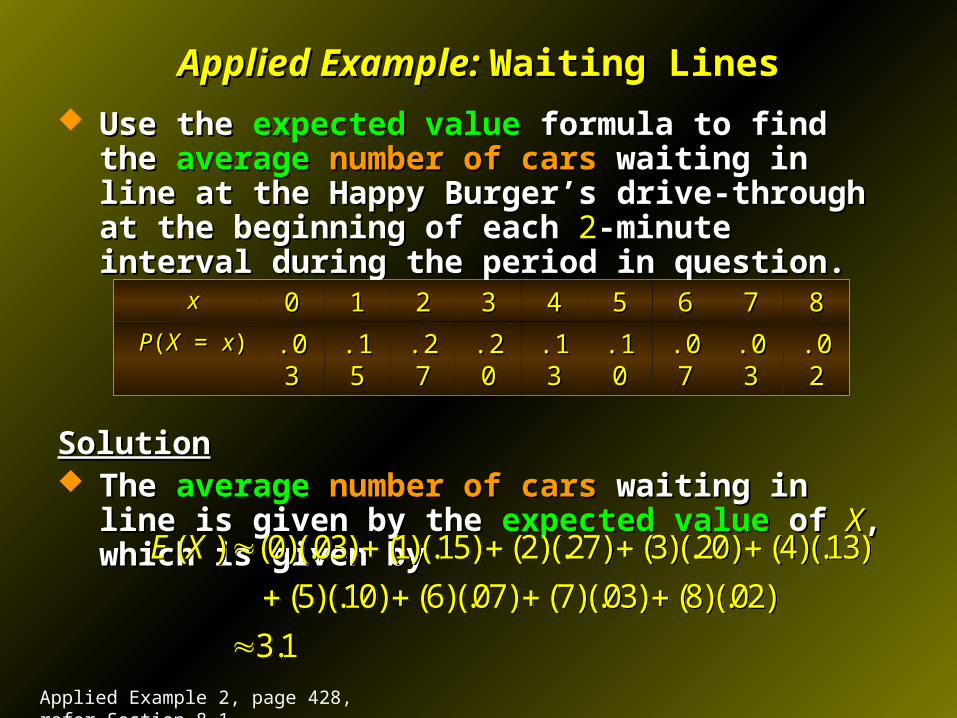
Applied Example: Applied Example: Waiting LinesWaiting Lines
Use the Use the expected valueexpected value formula to find the formula to find the averageaverage number of carsnumber of cars waiting in line at the Happy Burger’s waiting in line at the Happy Burger’s drive-through at the beginning of each drive-through at the beginning of each 22-minute interval -minute interval during the period in question.during the period in question.
SolutionSolution The The averageaverage number of carsnumber of cars waiting in line is given by the waiting in line is given by the
expected valueexpected value of of XX, which is given by, which is given by
( ) (0)(.03) (1)(.15) (2)(.27) (3)(.20) (4)(.13)
(5)(.10) (6)(.07) (7)(.03) (8)(.02)
3.1
E X
( ) (0)(.03) (1)(.15) (2)(.27) (3)(.20) (4)(.13)
(5)(.10) (6)(.07) (7)(.03) (8)(.02)
3.1
E X
xx 00 11 22 33 44 55 66 77 88
PP((XX = = xx)) .03.03 .15.15 .27.27 .20.20 .13.13 .10.10 .07.07 .03.03 .02.02
Applied Example 2, page 428, refer Section 8.1
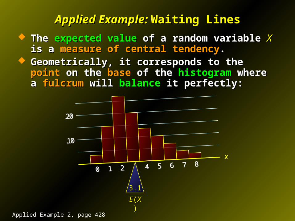
Applied Example: Applied Example: Waiting LinesWaiting Lines
The The expected valueexpected value of a random variable of a random variable XX is a is a measure of measure of central tendencycentral tendency..
Geometrically, it corresponds to the Geometrically, it corresponds to the pointpoint on the on the basebase of of the the histogramhistogram where a where a fulcrumfulcrum will will balancebalance it perfectly: it perfectly:
00 11 22 44 55 66 77 88
.20.20
.10.10
xx
3.13.1
EE((XX))
Applied Example 2, page 428
Applied Example:Applied Example: Raffles Raffles
The Island Club is holding a fundraising raffle.The Island Club is holding a fundraising raffle. Ten thousandTen thousand tickets have been sold for tickets have been sold for $2$2 each. each. There will be a There will be a first prizefirst prize of of $3000$3000, , 33 second prizessecond prizes of of
$1000$1000 each, each, 55 third prizesthird prizes of of $500$500 each, and each, and 2020 consolation prizesconsolation prizes of of $100$100 each. each.
Letting Letting XX denote the denote the net winningsnet winnings (winnings less the cost (winnings less the cost of the ticket) associated with the tickets, find of the ticket) associated with the tickets, find EE((XX))..
Interpret your results.Interpret your results.
Applied Example 5, page 431
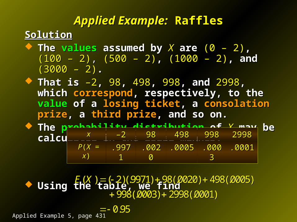
Applied Example:Applied Example: Raffles RafflesSolutionSolution The The valuesvalues assumed by assumed by XX are are (0 – 2)(0 – 2),, (100 – 2) (100 – 2),, (500 – 2) (500 – 2),,
(1000 – 2)(1000 – 2), and, and (3000 – 2) (3000 – 2). . That is That is –2–2, , 9898, , 498498, , 998998, and , and 29982998, which , which correspondcorrespond, ,
respectively, to the respectively, to the valuevalue of aof a losing ticket losing ticket, a , a consolation consolation prizeprize, a , a third prizethird prize, and so on., and so on.
The The probability distributionprobability distribution of of XX may be calculated in may be calculated in the usual manner:the usual manner:
Using the table, we findUsing the table, we find
xx ––22 9898 498498 998998 29982998
PP((XX = = xx)) .9971.9971 .0020.0020 .0005.0005 .0003.0003 .0001.0001
( ) ( 2)(.9971) 98(.0020) 498(.0005)
998(.0003) 2998(.0001)
0.95
E X
( ) ( 2)(.9971) 98(.0020) 498(.0005)
998(.0003) 2998(.0001)
0.95
E X
Applied Example 5, page 431
Applied Example:Applied Example: Raffles RafflesSolutionSolution The expected value of The expected value of EE((XX) = –.95) = –.95 gives the gives the long-run long-run
average lossaverage loss (negative gain) of a holder of one ticket. (negative gain) of a holder of one ticket. That is, if one participated That is, if one participated regularlyregularly in such a raffle by in such a raffle by
purchasing one ticket each time, in the long-run, purchasing one ticket each time, in the long-run, one one may expect to lose, on average,may expect to lose, on average, 9595 cents per raffle. cents per raffle.
Applied Example 5, page 431
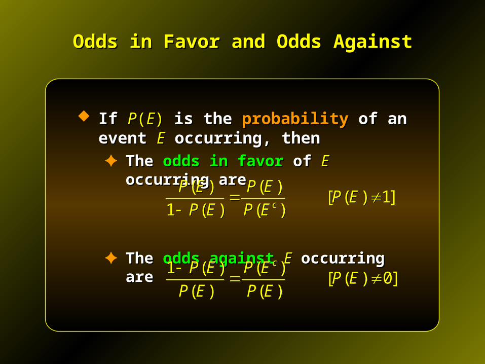
Odds in Favor and Odds AgainstOdds in Favor and Odds Against
If If PP((EE)) is the is the probabilityprobability of an event of an event EE occurring, thenoccurring, then✦ The The odds in favorodds in favor of of EE occurring are occurring are
✦ The The odds againstodds against EE occurring are occurring are
( ) ( )[ ( ) 1]
1 ( ) ( )c
P E P EP E
P E P E
( ) ( )[ ( ) 1]
1 ( ) ( )c
P E P EP E
P E P E
1 ( ) ( )[ ( ) 0]
( ) ( )
cP E P EP E
P E P E
1 ( ) ( )[ ( ) 0]
( ) ( )
cP E P EP E
P E P E
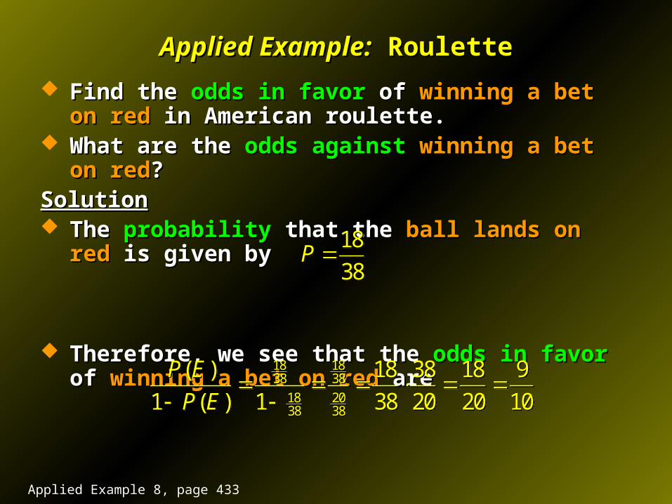
Applied Example:Applied Example: Roulette Roulette
Find the Find the odds in favorodds in favor of of winning a bet on redwinning a bet on red in in American roulette.American roulette.
What are the What are the odds againstodds against winning a bet on redwinning a bet on red??SolutionSolution The The probabilityprobability that the that the ball lands on redball lands on red is given by is given by
Therefore, we see that the Therefore, we see that the odds in favorodds in favor of of winning a bet winning a bet on redon red are are
18
38P
18
38P
18 1838 38
18 2038 38
( ) 18 38 18 9
1 ( ) 1 38 20 20 10
P E
P E
18 1838 38
18 2038 38
( ) 18 38 18 9
1 ( ) 1 38 20 20 10
P E
P E
Applied Example 8, page 433
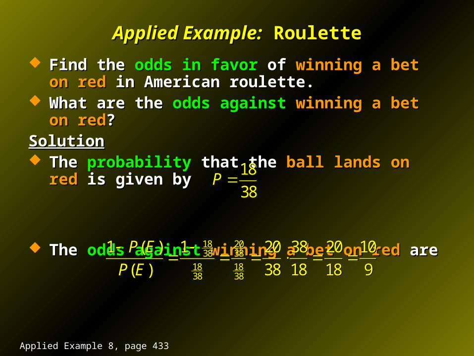
Applied Example:Applied Example: Roulette Roulette
Find the Find the odds in favorodds in favor of of winning a bet on redwinning a bet on red in in American roulette.American roulette.
What are the What are the odds againstodds against winning a bet on redwinning a bet on red??SolutionSolution The The probabilityprobability that the that the ball lands on redball lands on red is given by is given by
The The odds againstodds against winning a bet on redwinning a bet on red are are
18
38P
18
38P
18 2038 38
18 1838 38
1 ( ) 1 20 38 20 10
( ) 38 18 18 9
P E
P E
18 2038 38
18 1838 38
1 ( ) 1 20 38 20 10
( ) 38 18 18 9
P E
P E
Applied Example 8, page 433
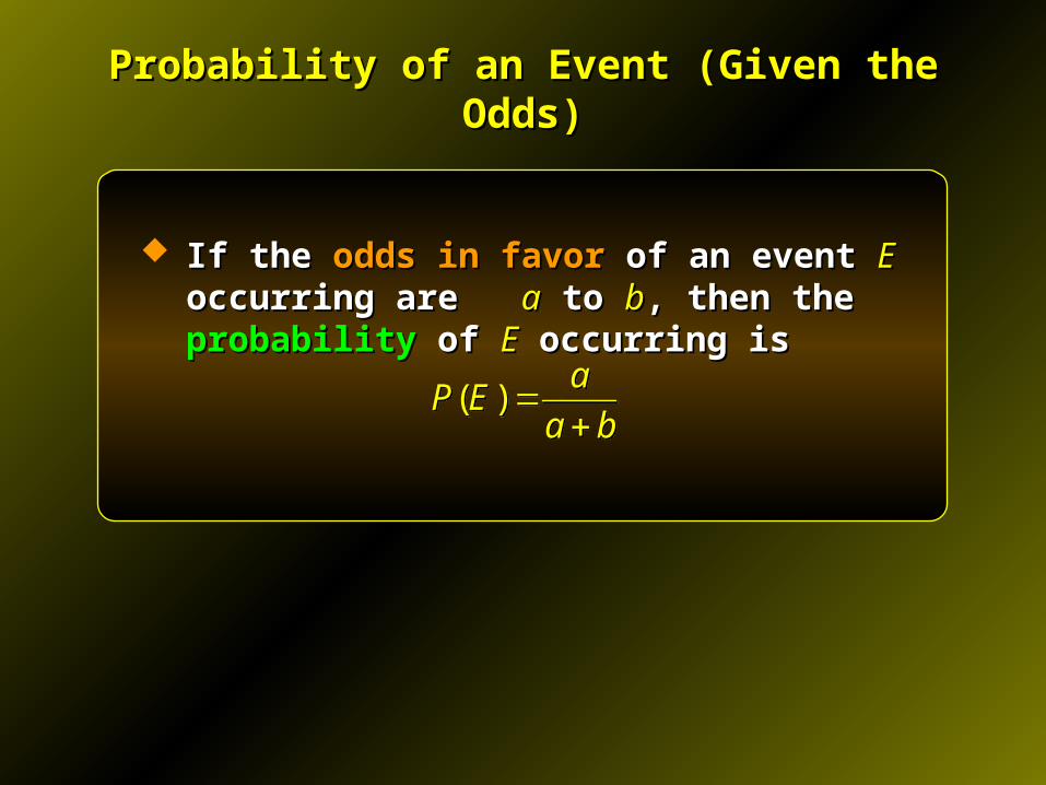
Probability of an Event (Given the Odds)Probability of an Event (Given the Odds)
If the If the odds in favorodds in favor of an event of an event E E occurring are occurring are aa to to bb, then the , then the probabilityprobability of of EE occurring is occurring is
( )a
P Ea b
( )a
P Ea b
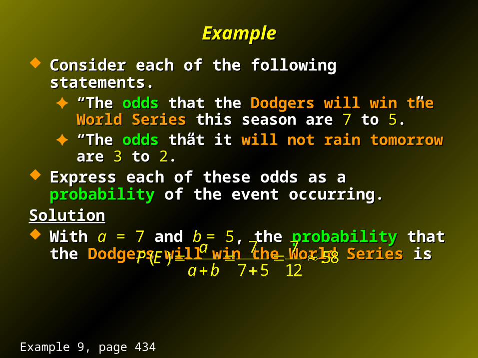
ExampleExample
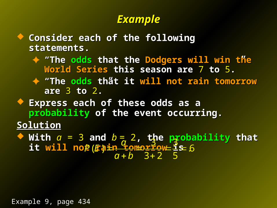
Consider each of the following statements.Consider each of the following statements.✦ ““The The oddsodds that the that the Dodgers will win the World SeriesDodgers will win the World Series
this season are this season are 77 to to 55.”.”✦ ““The The oddsodds that it that it will not rain tomorrowwill not rain tomorrow are are 33 to to 22.”.”
Express each of these odds as a Express each of these odds as a probabilityprobability of the event of the event occurring.occurring.
SolutionSolution With With aa = 7 = 7 and and b b = 5= 5, the , the probabilityprobability that the that the Dodgers will Dodgers will
win the World Serieswin the World Series is is
7 7( ) .58
7 5 12
aP E
a b
7 7
( ) .587 5 12
aP E
a b
Example 9, page 434
ExampleExample
Consider each of the following statements.Consider each of the following statements.✦ ““The The oddsodds that the that the Dodgers will win the World SeriesDodgers will win the World Series
this season are this season are 77 to to 55.”.”✦ ““The The oddsodds that it that it will not rain tomorrowwill not rain tomorrow are are 33 to to 22.”.”
Express each of these odds as a Express each of these odds as a probabilityprobability of the event of the event occurring.occurring.
SolutionSolution With With aa = 3 = 3 and and b b = 2= 2, the , the probabilityprobability that it that it will not rain will not rain
tomorrowtomorrow is is
3 3( ) .6
3 2 5
aP E
a b
3 3
( ) .63 2 5
aP E
a b
Example 9, page 434
MedianMedian
The The medianmedian of a group of numbers arranged of a group of numbers arranged in increasing or decreasing order is in increasing or decreasing order is
a.a. The The middle numbermiddle number if there is an if there is an oddodd number of entries or number of entries or
b.b. The The mean of the two middle numbersmean of the two middle numbers if if there is an there is an eveneven number of entries. number of entries.
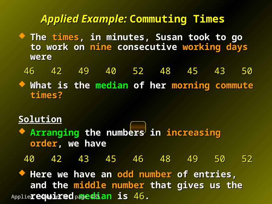
Applied Example: Applied Example: Commuting Times Commuting Times
The The timestimes, in minutes, Susan took to go to work on , in minutes, Susan took to go to work on nine nine consecutiveconsecutive working days working days were were
46 42 49 40 52 48 45 43 5046 42 49 40 52 48 45 43 50
What is the What is the medianmedian of her of her morning commute times?morning commute times?
SolutionSolution ArrangingArranging the numbers in the numbers in increasing orderincreasing order, we have, we have
40 42 43 45 46 48 49 50 5240 42 43 45 46 48 49 50 52
Here we have an Here we have an odd numberodd number of entries, and the of entries, and the middle middle numbernumber that gives us the required that gives us the required medianmedian is is 4646..
Applied Example 10, page 435
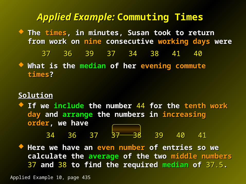
Applied Example: Applied Example: Commuting Times Commuting Times
The The timestimes, in minutes, Susan took to return from work on , in minutes, Susan took to return from work on nine nine consecutiveconsecutive working days working days were were
37 36 39 37 34 38 41 40 37 36 39 37 34 38 41 40
What is the What is the medianmedian of her of her evening commute timesevening commute times??
SolutionSolution If weIf we include include the numberthe number 4444 for the for the tenth work daytenth work day and and
arrangearrange the numbers in the numbers in increasing orderincreasing order, we have, we have
34 36 37 37 38 39 40 4134 36 37 37 38 39 40 41
Here we have an Here we have an even numbereven number of entries so we calculate of entries so we calculate the the averageaverage of the two of the two middle numbers middle numbers 3737 andand 3838 to find to find the required the required medianmedian of of 37.537.5..
Applied Example 10, page 435

ModeMode
The mode of a group of numbers is the The mode of a group of numbers is the number in the set that occurs most number in the set that occurs most frequently.frequently.
ExampleExample
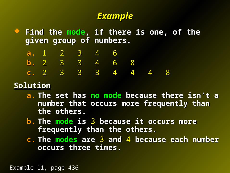
Find the Find the modemode, if there is one, of the given group of , if there is one, of the given group of numbers.numbers.
a.a. 1 2 3 4 61 2 3 4 6b.b. 2 3 3 4 6 82 3 3 4 6 8c.c. 2 3 3 3 4 4 4 82 3 3 3 4 4 4 8
SolutionSolutiona.a. The set has The set has no modeno mode because there isn’t a number that because there isn’t a number that
occurs more frequently than the others.occurs more frequently than the others.
b.b. The The modemode is is 33 because it occurs more frequently than the because it occurs more frequently than the others.others.
c.c. The The modesmodes are are 33 and and 44 because each number occurs three because each number occurs three times.times.
Example 11, page 436
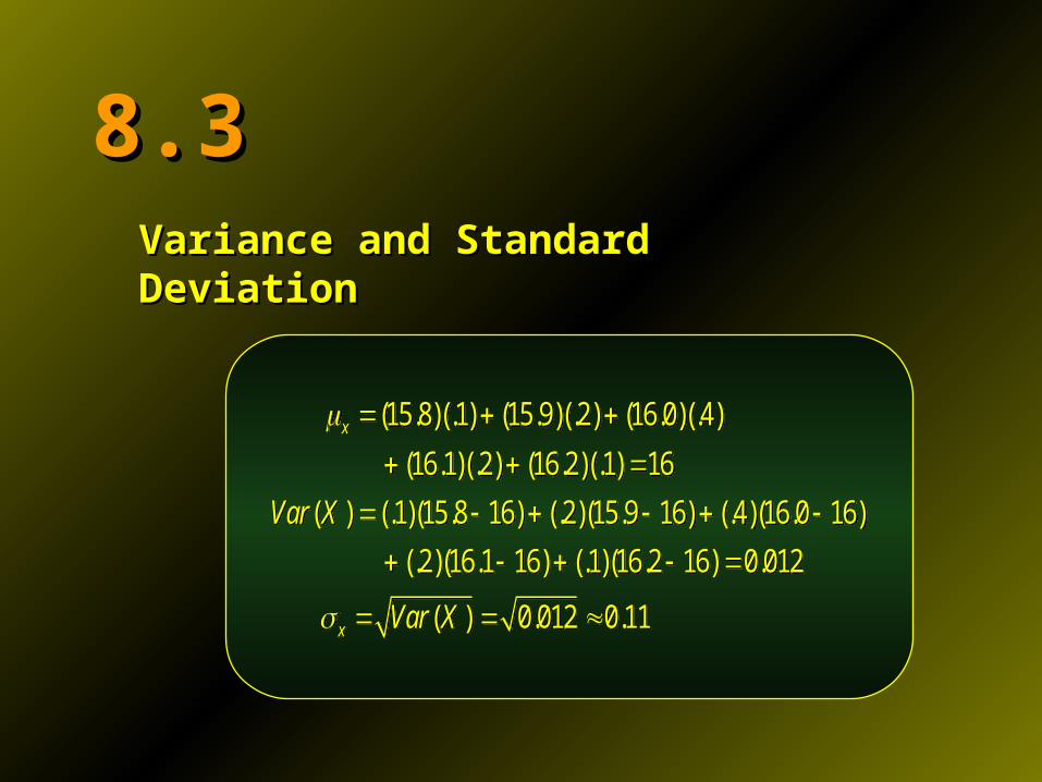
8.38.3Variance and Standard DeviationVariance and Standard Deviation
(15.8)(.1) (15.9)(.2) (16.0)(.4)
(16.1)(.2) (16.2)(.1) 16
( ) (.1)(15.8 16) (.2)(15.9 16) (.4)(16.0 16)
(.2)(16.1 16) (.1)(16.2 16) 0.012
( ) 0
x
x
Var X
Var X
.012 0.11
(15.8)(.1) (15.9)(.2) (16.0)(.4)
(16.1)(.2) (16.2)(.1) 16
( ) (.1)(15.8 16) (.2)(15.9 16) (.4)(16.0 16)
(.2)(16.1 16) (.1)(16.2 16) 0.012
( ) 0
x
x
Var X
Var X
.012 0.11
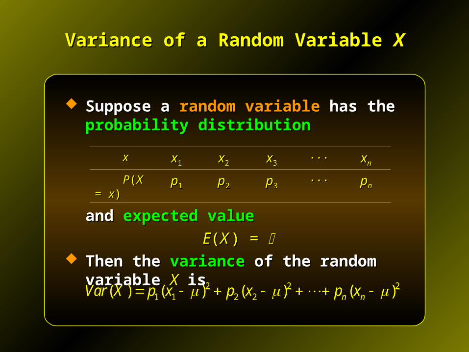
Variance of a Random Variable Variance of a Random Variable XX
Suppose a Suppose a random variablerandom variable has the has the probability probability distributiondistribution
and and expected valueexpected value
EE((XX ) = ) = Then the Then the variancevariance of the random variable of the random variable XX is is
xx xx11 xx22 xx33 · · ·· · · xxnn
PP((XX = = xx)) pp11 pp22 pp33 · · ·· · · ppnn
2 2 21 1 2 2( ) ( ) ( ) ( )n nVar X p x p x p x 2 2 21 1 2 2( ) ( ) ( ) ( )n nVar X p x p x p x
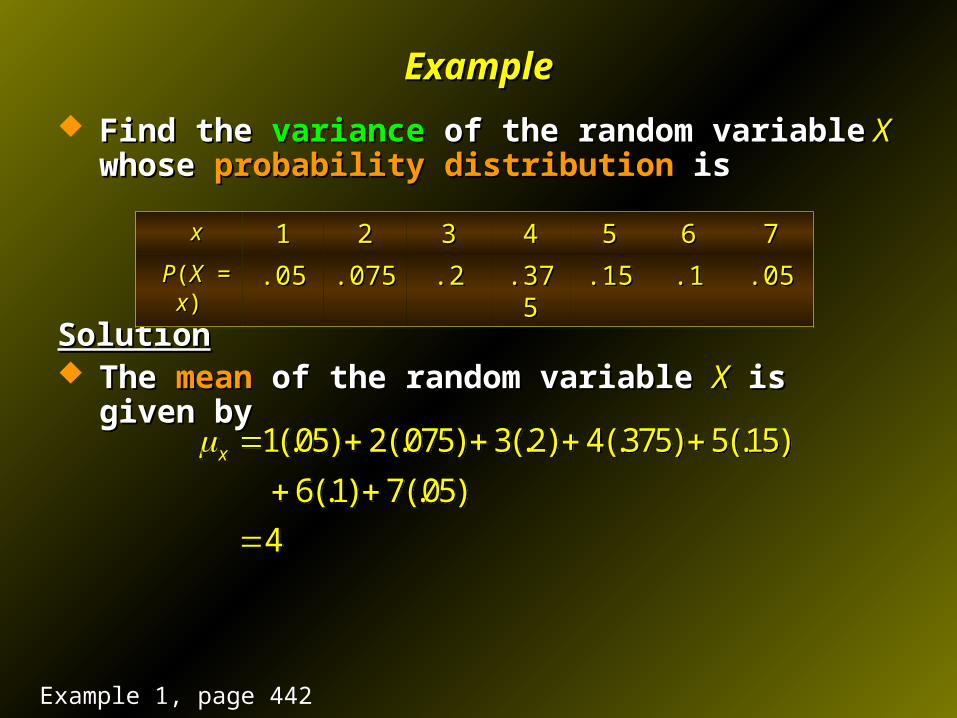
ExampleExample
Find the Find the variancevariance of the random variable of the random variable X X whose whose probability distributionprobability distribution is is
SolutionSolution The The meanmean of the random variable of the random variable XX is given by is given by
xx 11 22 33 44 55 66 77
PP((XX = = xx))
.05.05 .075.075 .2.2 .375.375 .15.15 .1.1 .05.05
1(.05) 2(.075) 3(.2) 4(.375) 5(.15)
6(.1) 7(.05)
4
x
1(.05) 2(.075) 3(.2) 4(.375) 5(.15)
6(.1) 7(.05)
4
x
Example 1, page 442

ExampleExample
Find the Find the variancevariance of the random variable of the random variable X X whose whose probability distributionprobability distribution is is
SolutionSolution Therefore, the Therefore, the variancevariance of of XX is given by is given by
xx 11 22 33 44 55 66 77
PP((XX = = xx))
.05.05 .075.075 .2.2 .375.375 .15.15 .1.1 .05.05
2 2 2
2 2
2 2
( ) (.05)(1 4) (.075)(2 4) (.2)(3 4)
(.375)(4 4) (.15)(5 4)
(.1)(6 4) (.05)(7 4)
1.95
Var X
2 2 2
2 2
2 2
( ) (.05)(1 4) (.075)(2 4) (.2)(3 4)
(.375)(4 4) (.15)(5 4)
(.1)(6 4) (.05)(7 4)
1.95
Var X
Example 1, page 442
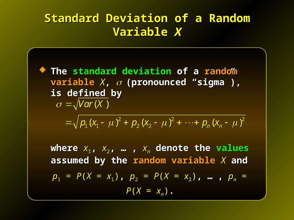
Standard Deviation of a Random Variable Standard Deviation of a Random Variable XX
The The standard deviationstandard deviation of a of a random variablerandom variable XX, , (pronounced “sigma”), is defined by(pronounced “sigma”), is defined by
where where xx11, , xx22, … , , … , xxnn denote the denote the valuesvalues assumed by assumed by
the the random variablerandom variable XX and and
pp11 = = PP((XX = = xx11)), , pp22 = = PP((XX = = xx22)), … , , … , ppnn = = PP((XX = = xxnn))..
2 2 21 1 2 2
( )
( ) ( ) ( )n n
Var X
p x p x p x
2 2 21 1 2 2
( )
( ) ( ) ( )n n
Var X
p x p x p x
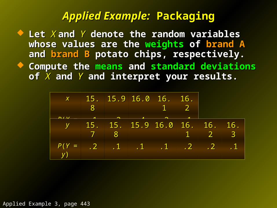
Let Let X X and and YY denote the random variables whose values are denote the random variables whose values are the the weightsweights of of brand Abrand A and and brand Bbrand B potato chips, potato chips, respectively. respectively.
Compute the Compute the meansmeans and and standard deviationsstandard deviations of of XX and and YY and interpret your results.and interpret your results.
xx 15.815.8 15.915.9 16.016.0 16.116.1 16.216.2
PP((XX = = xx)) .1.1 .2.2 .4.4 .2.2 .1.1
yy 15.715.7 15.815.8 15.915.9 16.016.0 16.116.1 16.216.2 16.316.3
PP((YY = = yy)) .2.2 .1.1 .1.1 .1.1 .2.2 .2.2 .1.1
Applied Example:Applied Example: Packaging Packaging
Applied Example 3, page 443
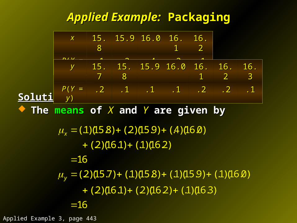
Applied Example:Applied Example: Packaging Packaging
SolutionSolution The The meansmeans of of XX and and YY are given by are given by
xx 15.815.8 15.915.9 16.016.0 16.116.1 16.216.2
PP((XX = = xx)) .1.1 .2.2 .4.4 .2.2 .1.1
yy 15.715.7 15.815.8 15.915.9 16.016.0 16.116.1 16.216.2 16.316.3
PP((YY = = yy)) .2.2 .1.1 .1.1 .1.1 .2.2 .2.2 .1.1
(.1)(15.8) (.2)(15.9) (.4)(16.0)
(.2)(16.1) (.1)(16.2)
16
(.2)(15.7) (.1)(15.8) (.1)(15.9) (.1)(16.0)
(.2)(16.1) (.2)(16.2) (.1)(16.3)
16
x
y
(.1)(15.8) (.2)(15.9) (.4)(16.0)
(.2)(16.1) (.1)(16.2)
16
(.2)(15.7) (.1)(15.8) (.1)(15.9) (.1)(16.0)
(.2)(16.1) (.2)(16.2) (.1)(16.3)
16
x
y
Applied Example 3, page 443
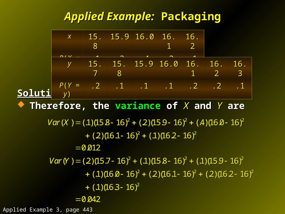
Applied Example:Applied Example: Packaging Packaging
SolutionSolution Therefore, the Therefore, the variancevariance of of XX and and YY are are
xx 15.815.8 15.915.9 16.016.0 16.116.1 16.216.2
PP((XX = = xx)) .1.1 .2.2 .4.4 .2.2 .1.1
yy 15.715.7 15.815.8 15.915.9 16.016.0 16.116.1 16.216.2 16.316.3
PP((YY = = yy)) .2.2 .1.1 .1.1 .1.1 .2.2 .2.2 .1.1
2 2 2
2 2
2 2 2
2 2 2
( ) (.1)(15.8 16) (.2)(15.9 16) (.4)(16.0 16)
(.2)(16.1 16) (.1)(16.2 16)
0.012
( ) (.2)(15.7 16) (.1)(15.8 16) (.1)(15.9 16)
(.1)(16.0 16) (.2)(16.1 16) (.2)(16.2 16)
(.1)(16
Var X
Var Y
2.3 16)
0.042
2 2 2
2 2
2 2 2
2 2 2
( ) (.1)(15.8 16) (.2)(15.9 16) (.4)(16.0 16)
(.2)(16.1 16) (.1)(16.2 16)
0.012
( ) (.2)(15.7 16) (.1)(15.8 16) (.1)(15.9 16)
(.1)(16.0 16) (.2)(16.1 16) (.2)(16.2 16)
(.1)(16
Var X
Var Y
2.3 16)
0.042
Applied Example 3, page 443
Applied Example:Applied Example: Packaging Packaging
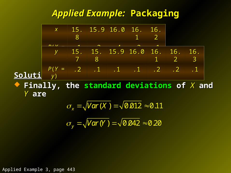
SolutionSolution Finally, the Finally, the standard deviationsstandard deviations of of XX and and YY are are
xx 15.815.8 15.915.9 16.016.0 16.116.1 16.216.2
PP((XX = = xx)) .1.1 .2.2 .4.4 .2.2 .1.1
yy 15.715.7 15.815.8 15.915.9 16.016.0 16.116.1 16.216.2 16.316.3
PP((YY = = yy)) .2.2 .1.1 .1.1 .1.1 .2.2 .2.2 .1.1
( ) 0.012 0.11
( ) 0.042 0.20
x
y
Var X
Var Y
( ) 0.012 0.11
( ) 0.042 0.20
x
y
Var X
Var Y
Applied Example 3, page 443
Applied Example:Applied Example: Packaging Packaging
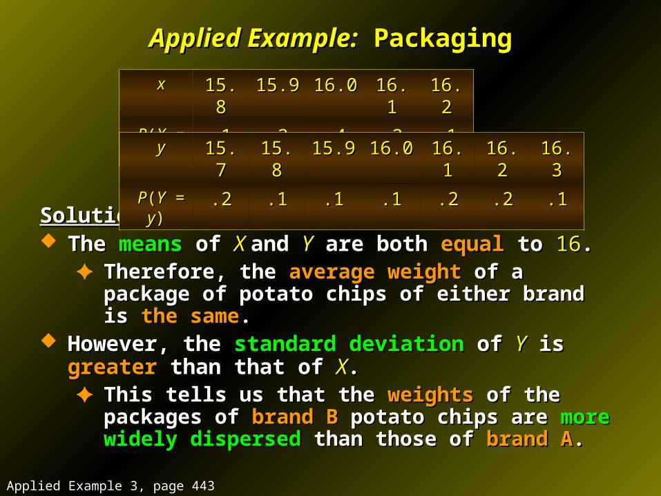
SolutionSolution The The meansmeans of of X X and and YY are both are both equalequal to to 1616. .
✦ Therefore, the Therefore, the average weightaverage weight of a package of potato of a package of potato chips of either brand is chips of either brand is the samethe same..
However, the However, the standard deviationstandard deviation of of YY is is greatergreater than that than that of of XX. . ✦ This tells us that the This tells us that the weightsweights of the packages of of the packages of brand Bbrand B
potato chips are potato chips are more widely dispersedmore widely dispersed than those of than those of brand Abrand A..
xx 15.815.8 15.915.9 16.016.0 16.116.1 16.216.2
PP((XX = = xx)) .1.1 .2.2 .4.4 .2.2 .1.1
yy 15.715.7 15.815.8 15.915.9 16.016.0 16.116.1 16.216.2 16.316.3
PP((YY = = yy)) .2.2 .1.1 .1.1 .1.1 .2.2 .2.2 .1.1
Applied Example 3, page 443
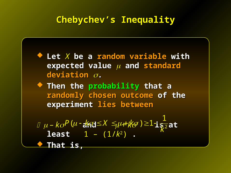
Chebychev’s InequalityChebychev’s Inequality
Let Let XX be a be a random variablerandom variable with expected with expected value value and and standard deviationstandard deviation ..
Then the Then the probabilityprobability that a that a randomly chosen randomly chosen outcomeoutcome of the experiment of the experiment lies betweenlies between
– – kk and and + k + k is at least is at least 1 – (1/1 – (1/kk22)) . . That is,That is,
2
1( ) 1P k X k
k 2
1( ) 1P k X k
k
Applied Example:Applied Example: Industrial Accidents Industrial Accidents
Great Lumber Co. employs Great Lumber Co. employs 400400 workers in its mills. workers in its mills. It has been estimated that It has been estimated that XX, the random variable , the random variable
measuring the measuring the number of mill workersnumber of mill workers who have who have industrial accidentsindustrial accidents during a during a 11-year period, is distributed -year period, is distributed with a with a meanmean of of 4040 and a and a standard deviationstandard deviation of of 66..
Use Use Chebychev’s InequalityChebychev’s Inequality to find a bound on the to find a bound on the probabilityprobability that the that the number of workersnumber of workers who will have an who will have an industrial industrial accidentaccident over a over a 11-year period is -year period is betweenbetween 3030 and and 5050, inclusive., inclusive.
Applied Example 5, page 445
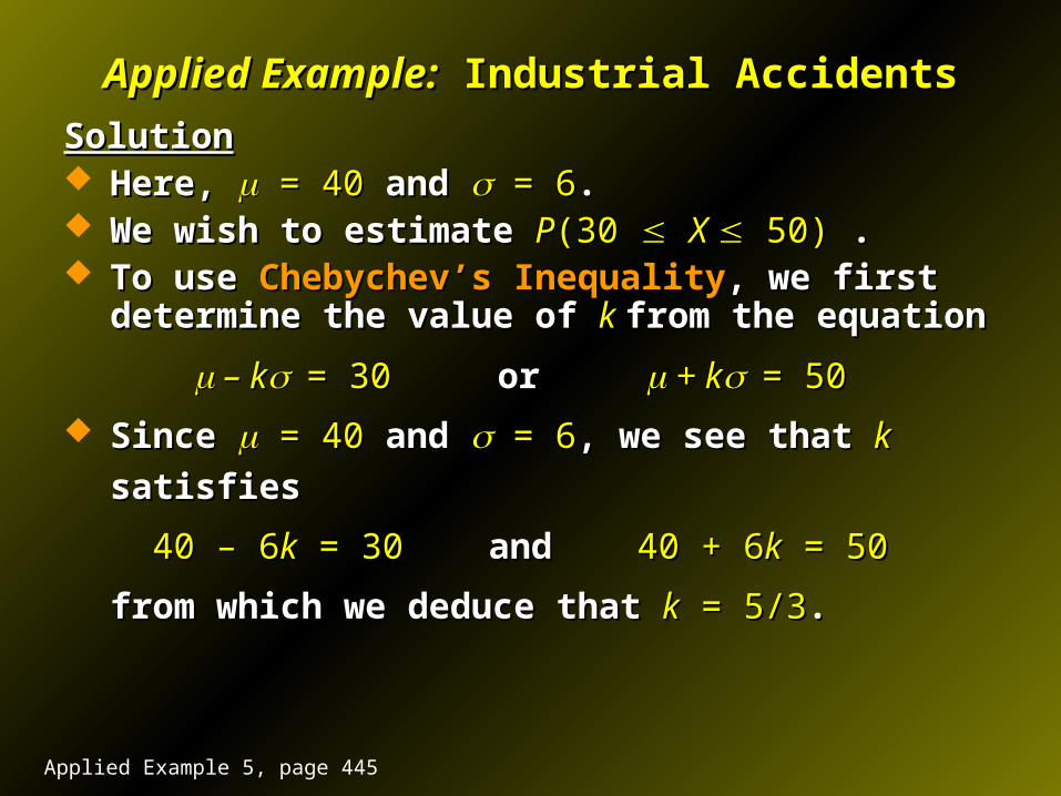
Applied Example:Applied Example: Industrial Accidents Industrial Accidents
SolutionSolution Here, Here, = 40 = 40 and and = 6= 6.. We wish to estimate We wish to estimate PP(30 (30 X X 50) 50) . . To use To use Chebychev’s InequalityChebychev’s Inequality, we first determine the , we first determine the
value of value of k k from the equationfrom the equation
– – kk= 30= 30 or or + k + k= 50= 50
Since Since = 40= 40 and and = 6= 6, we see that , we see that k k satisfiessatisfies
40 – 640 – 6kk = 30 = 30 and and 40 + 640 + 6kk = 50 = 50
from which we deduce that from which we deduce that kk = 5/3 = 5/3. .
Applied Example 5, page 445
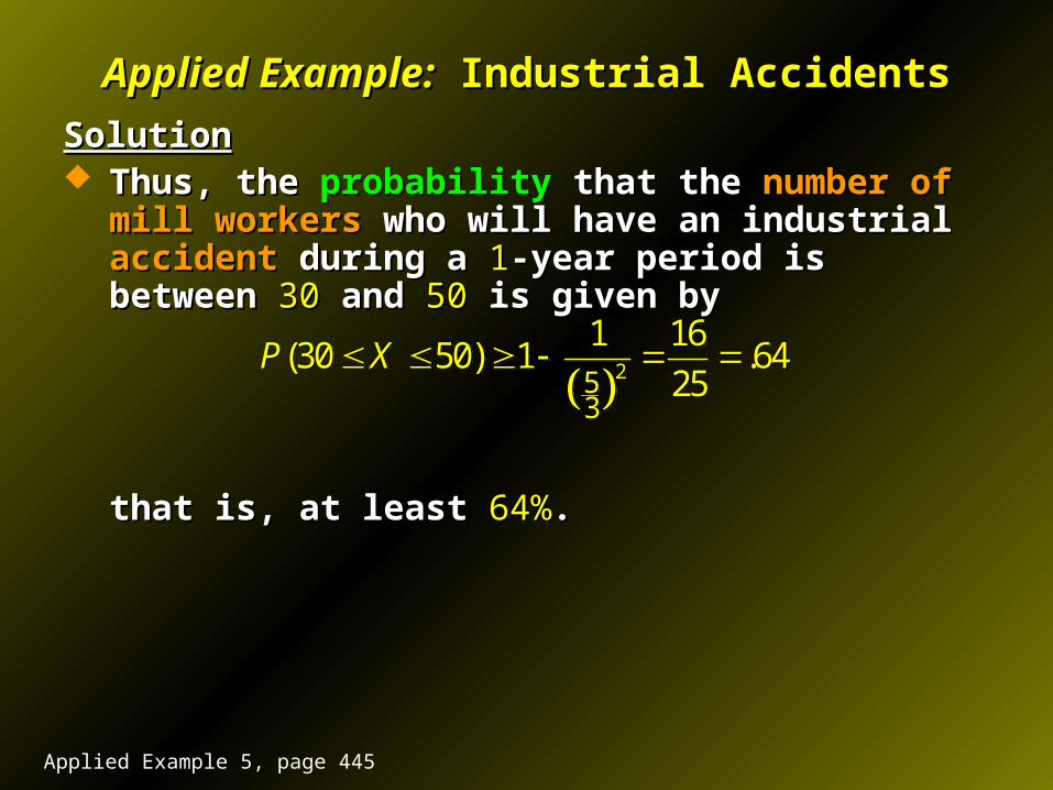
Applied Example:Applied Example: Industrial Accidents Industrial Accidents
SolutionSolution Thus, the Thus, the probabilityprobability that the that the number of mill workersnumber of mill workers who who
will have an industrial will have an industrial accidentaccident during a during a 11-year period is -year period is between between 3030 and and 5050 is given by is given by
that is, at least that is, at least 64%64%..
253
1 16(30 50) 1 .64
25P X
253
1 16(30 50) 1 .64
25P X
Applied Example 5, page 445
8.48.4The Binomial DistributionThe Binomial Distribution
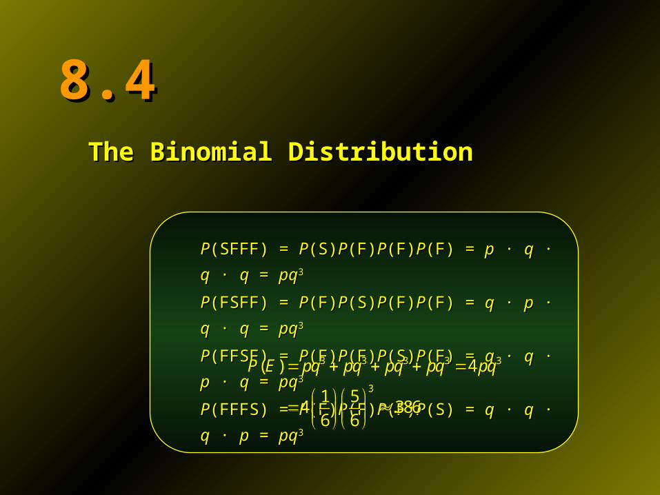
PP(SFFF) = (SFFF) = PP(S)(S)PP(F)(F)PP(F)(F)PP(F) = (F) = pp · · qq · · qq · · qq = = pqpq33
PP(FSFF) = (FSFF) = PP(F)(F)PP(S)(S)PP(F)(F)PP(F) = (F) = qq · · pp · · qq · · qq = = pqpq33
PP(FFSF) = (FFSF) = PP(F)(F)PP(F)(F)PP(S)(S)PP(F) = (F) = qq · · qq · · pp · · qq = = pqpq33
PP(FFFS) = (FFFS) = PP(F)(F)PP(F)(F)PP(F)(F)PP(S) = (S) = qq · · qq · · qq · · pp = = pqpq33
3 3 3 3 3
3
( ) 4
1 54 .386
6 6
P E pq pq pq pq pq
3 3 3 3 3
3
( ) 4
1 54 .386
6 6
P E pq pq pq pq pq
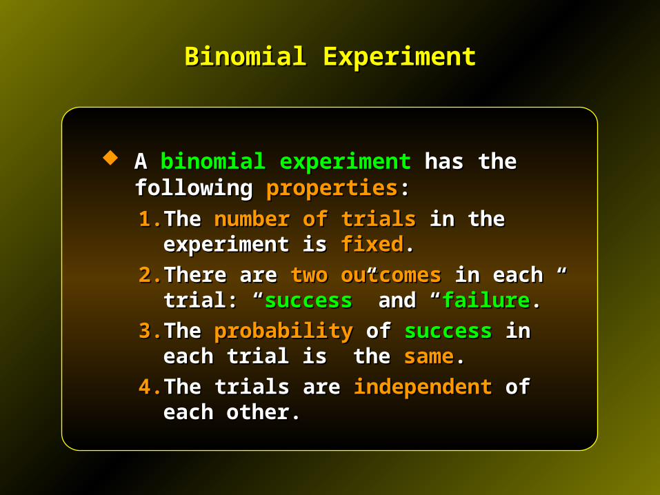
Binomial ExperimentBinomial Experiment
A A binomial experimentbinomial experiment has the following has the following propertiesproperties::
1.1. The The number of trialsnumber of trials in the experiment is in the experiment is fixedfixed..
2.2. There are There are two outcomestwo outcomes in each trial: in each trial: ““successsuccess” and “” and “failurefailure.”.”
3.3. The The probability probability ofof successsuccess in each trial is in each trial is the the samesame..
4.4. The trials are The trials are independentindependent of each other. of each other.
ExampleExample
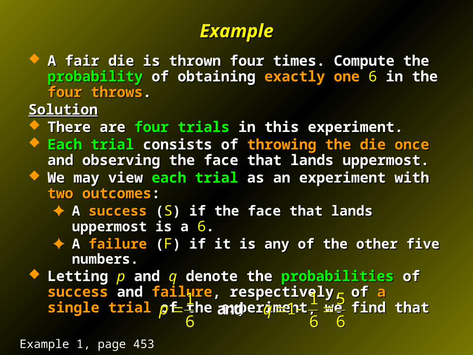
A fair die is thrown four times. Compute the A fair die is thrown four times. Compute the probabilityprobability of obtaining of obtaining exactly oneexactly one 66 in the in the four throwsfour throws..
SolutionSolution There are There are four trialsfour trials in this experiment. in this experiment. Each trialEach trial consists of consists of throwing the die oncethrowing the die once and observing and observing
the face that lands uppermost.the face that lands uppermost. We may view We may view each trialeach trial as an experiment with as an experiment with two two
outcomesoutcomes::✦ A A successsuccess ( (SS) if the face that lands uppermost is a ) if the face that lands uppermost is a 66..✦ A A failurefailure ( (FF) if it is any of the other five numbers.) if it is any of the other five numbers.
Letting Letting pp and and qq denote the denote the probabilities probabilities of of successsuccess and and failurefailure, respectively, of , respectively, of a single triala single trial of the experiment, we of the experiment, we find thatfind that
1 1 51
6 6 6p q and
1 1 51
6 6 6p q and
Example 1, page 453
ExampleExample
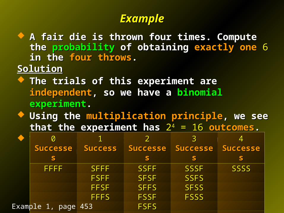
A fair die is thrown four times. Compute the A fair die is thrown four times. Compute the probabilityprobability of of obtaining obtaining exactly oneexactly one 66 in the in the four throwsfour throws..
SolutionSolution The trials of this experiment are The trials of this experiment are independentindependent, so we have a , so we have a
binomial experimentbinomial experiment.. Using the Using the multiplication principlemultiplication principle, we see that the , we see that the
experiment has experiment has 2244 = 16 = 16 outcomesoutcomes.. The The possible outcomespossible outcomes associated with the experiment are: associated with the experiment are:
00 Successes Successes 1 1 SuccessSuccess 22 Successes Successes 33 Successes Successes 44 Successes Successes
FFFFFFFF SFFFSFFF SSFFSSFF SSSFSSSF SSSSSSSSFSFFFSFF SFSFSFSF SSFSSSFSFFSFFFSF SFFSSFFS SFSSSFSSFFFSFFFS FSSFFSSF FSSSFSSS
FSFSFSFSFFSSFFSS
Example 1, page 453
00 Success Success 1 1 SuccessSuccess 22 Successes Successes 33 Successes Successes 44 Successes Successes
FFFFFFFF SFFFSFFF SSFFSSFF SSSFSSSF SSSSSSSSFSFFFSFF SFSFSFSF SSFSSSFSFFSFFFSF SFFSSFFS SFSSSFSSFFFSFFFS FSSFFSSF FSSSFSSS
FSFSFSFSFFSSFFSS
ExampleExample
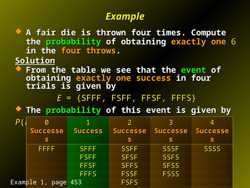
A fair die is thrown four times. Compute the A fair die is thrown four times. Compute the probabilityprobability of of obtaining obtaining exactly oneexactly one 66 in the in the four throwsfour throws..
SolutionSolution From the table we see that the From the table we see that the eventevent of obtaining of obtaining exactly exactly
one successone success in four trials is given by in four trials is given by
EE = {SFFF, FSFF, FFSF, FFFS} = {SFFF, FSFF, FFSF, FFFS} The The probabilityprobability of this event is given by of this event is given by
PP((EE) = ) = PP(SFFF) + (SFFF) + PP(FSFF) + (FSFF) + PP(FFSF) + (FFSF) + PP(FFFS) (FFFS)
00 Successes Successes 1 1 SuccessSuccess 22 Successes Successes 33 Successes Successes 44 Successes Successes
FFFFFFFF SFFFSFFF SSFFSSFF SSSFSSSF SSSSSSSSFSFFFSFF SFSFSFSF SSFSSSFSFFSFFFSF SFFSSFFS SFSSSFSSFFFSFFFS FSSFFSSF FSSSFSSS
FSFSFSFSFFSSFFSS
Example 1, page 453
ExampleExample
A fair die is thrown four times. Compute the A fair die is thrown four times. Compute the probabilityprobability of of obtaining obtaining exactly oneexactly one 66 in the in the four throwsfour throws..
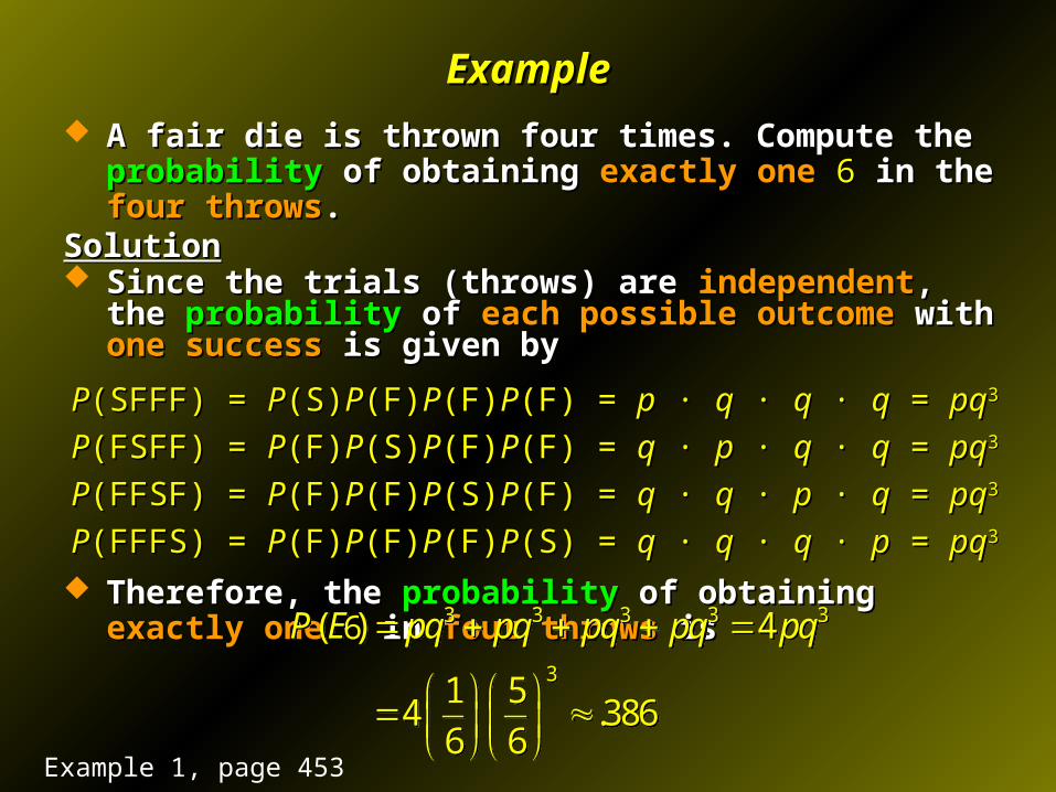
SolutionSolution Since the trials (throws) are Since the trials (throws) are independentindependent, the , the probabilityprobability of of
each possible outcomeeach possible outcome with with one successone success is given by is given by
PP(SFFF) = (SFFF) = PP(S)(S)PP(F)(F)PP(F)(F)PP(F) = (F) = pp · · qq · · qq · · qq = = pqpq33
PP(FSFF) = (FSFF) = PP(F)(F)PP(S)(S)PP(F)(F)PP(F) = (F) = qq · · pp · · qq · · qq = = pqpq33
PP(FFSF) = (FFSF) = PP(F)(F)PP(F)(F)PP(S)(S)PP(F) = (F) = qq · · qq · · pp · · qq = = pqpq33
PP(FFFS) = (FFFS) = PP(F)(F)PP(F)(F)PP(F)(F)PP(S) = (S) = qq · · qq · · qq · · pp = = pqpq33
Therefore, the Therefore, the probabilityprobability of obtaining of obtaining exactly oneexactly one 66 in in four four throwsthrows is is
3 3 3 3 3
3
( ) 4
1 54 .386
6 6
P E pq pq pq pq pq
3 3 3 3 3
3
( ) 4
1 54 .386
6 6
P E pq pq pq pq pq
Example 1, page 453
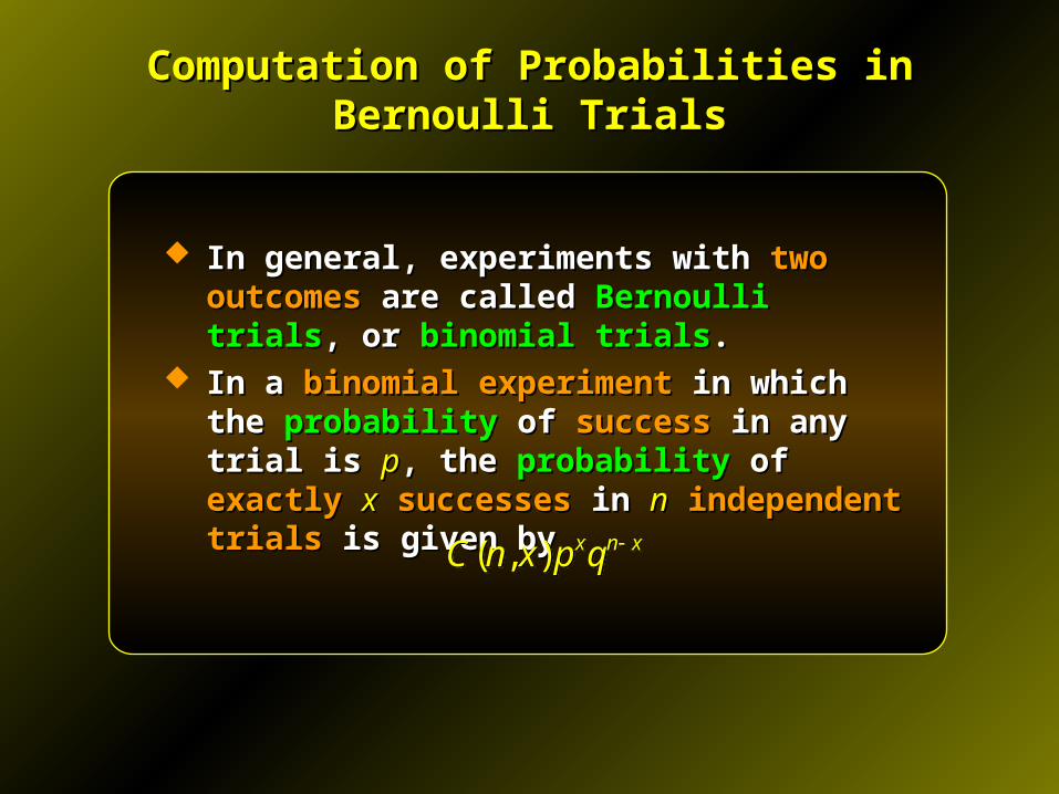
In general, experiments with In general, experiments with two outcomestwo outcomes are called are called Bernoulli trialsBernoulli trials, or , or binomial trialsbinomial trials..
In a In a binomial experimentbinomial experiment in which the in which the probabilityprobability ofof success success in any trial is in any trial is pp, the , the probabilityprobability of of exactlyexactly xx successessuccesses in in nn independent trialsindependent trials is given by is given by
Computation of Probabilities in Bernoulli TrialsComputation of Probabilities in Bernoulli Trials
( , ) x n xC n x p q ( , ) x n xC n x p q
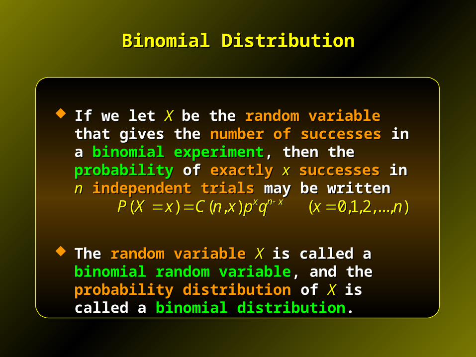
If we let If we let XX be the be the random variablerandom variable that gives the that gives the number of successesnumber of successes in a in a binomial experimentbinomial experiment, , then the then the probabilityprobability of of exactlyexactly xx successessuccesses in in nn independent trialsindependent trials may be written may be written
The The random variablerandom variable XX is called a is called a binomial binomial random variablerandom variable, and the , and the probability distributionprobability distribution of of XX is called a is called a binomial distributionbinomial distribution..
Binomial DistributionBinomial Distribution
( ) ( , ) ( 0,1,2,..., )x n xP X x C n x p q x n ( ) ( , ) ( 0,1,2,..., )x n xP X x C n x p q x n
ExampleExample
A fair die is thrown A fair die is thrown five timesfive times. . If a If a 11 or a or a 66 lands uppermost in a trial, then the throw is lands uppermost in a trial, then the throw is
considered a considered a successsuccess.. Otherwise, the throw is considered a Otherwise, the throw is considered a failurefailure.. Find the Find the probabilitiesprobabilities of obtaining of obtaining exactlyexactly 00, , 11, , 22, , 33, , 44, and , and 55
successessuccesses, in this experiment., in this experiment. Using the results obtained, construct the Using the results obtained, construct the binomial binomial
distributiondistribution for this experiment and draw the for this experiment and draw the histogramhistogram associated with it.associated with it.
Example 2, page 455
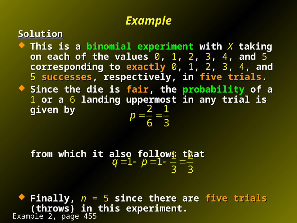
ExampleExampleSolutionSolution This is a This is a binomial experimentbinomial experiment with with XX taking on each of the taking on each of the
values values 00, , 11, , 22, , 33, , 44, and , and 55 corresponding to corresponding to exactlyexactly 00, , 11, , 22, , 33, , 44, and , and 55 successessuccesses, respectively, in , respectively, in five trialsfive trials..
Since the die is Since the die is fairfair, the , the probabilityprobability of a of a 11 or a or a 66 landing landing uppermost in any trial is given by uppermost in any trial is given by
from which it also follows thatfrom which it also follows that
Finally, Finally, nn = 5 = 5 since there are since there are five trialsfive trials (throws) in this (throws) in this experiment.experiment.
2 1
6 3p
2 1
6 3p
1 21 1
3 3q p
1 21 1
3 3q p
Example 2, page 455
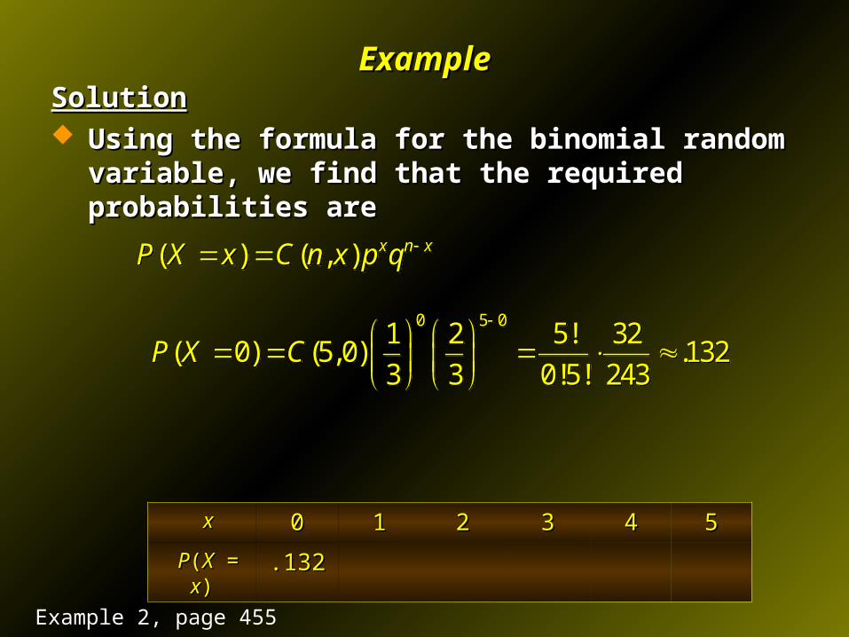
ExampleExampleSolutionSolution Using the formula for the binomial random variable, we Using the formula for the binomial random variable, we
find that the required probabilities arefind that the required probabilities are
( ) ( , ) x n xP X x C n x p q ( ) ( , ) x n xP X x C n x p q
0 5 01 2 5! 32
( 0) (5,0) .1323 3 0!5! 243
P X C
0 5 01 2 5! 32
( 0) (5,0) .1323 3 0!5! 243
P X C
xx 00 11 22 33 44 55
PP((XX = = xx)) .132.132
Example 2, page 455
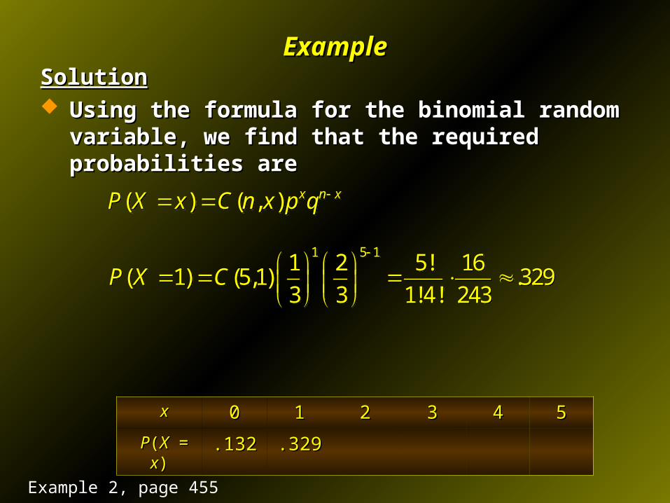
ExampleExampleSolutionSolution Using the formula for the binomial random variable, we Using the formula for the binomial random variable, we
find that the required probabilities arefind that the required probabilities are
( ) ( , ) x n xP X x C n x p q ( ) ( , ) x n xP X x C n x p q
1 5 11 2 5! 16
( 1) (5,1) .3293 3 1!4! 243
P X C
1 5 11 2 5! 16
( 1) (5,1) .3293 3 1!4! 243
P X C
xx 00 11 22 33 44 55
PP((XX = = xx)) .132.132 .329.329
Example 2, page 455

ExampleExampleSolutionSolution Using the formula for the binomial random variable, we Using the formula for the binomial random variable, we
find that the required probabilities arefind that the required probabilities are
( ) ( , ) x n xP X x C n x p q ( ) ( , ) x n xP X x C n x p q
2 5 21 2 5! 8
( 2) (5,2) .3293 3 2!3! 243
P X C
2 5 21 2 5! 8
( 2) (5,2) .3293 3 2!3! 243
P X C
xx 00 11 22 33 44 55
PP((XX = = xx)) .132.132 .329.329 329329
Example 2, page 455

ExampleExampleSolutionSolution Using the formula for the binomial random variable, we Using the formula for the binomial random variable, we
find that the required probabilities arefind that the required probabilities are
( ) ( , ) x n xP X x C n x p q ( ) ( , ) x n xP X x C n x p q
3 5 31 2 5! 4
( 3) (5,3) .1653 3 3!2! 243
P X C
3 5 31 2 5! 4
( 3) (5,3) .1653 3 3!2! 243
P X C
xx 00 11 22 33 44 55
PP((XX = = xx)) .132.132 .329.329 329329 .165.165
Example 2, page 455

ExampleExampleSolutionSolution Using the formula for the binomial random variable, we Using the formula for the binomial random variable, we
find that the required probabilities arefind that the required probabilities are
( ) ( , ) x n xP X x C n x p q ( ) ( , ) x n xP X x C n x p q
4 5 41 2 5! 2
( 4) (5,4) .0413 3 4!1! 243
P X C
4 5 41 2 5! 2
( 4) (5,4) .0413 3 4!1! 243
P X C
xx 00 11 22 33 44 55
PP((XX = = xx)) .132.132 .329.329 329329 .165.165 .041.041
Example 2, page 455
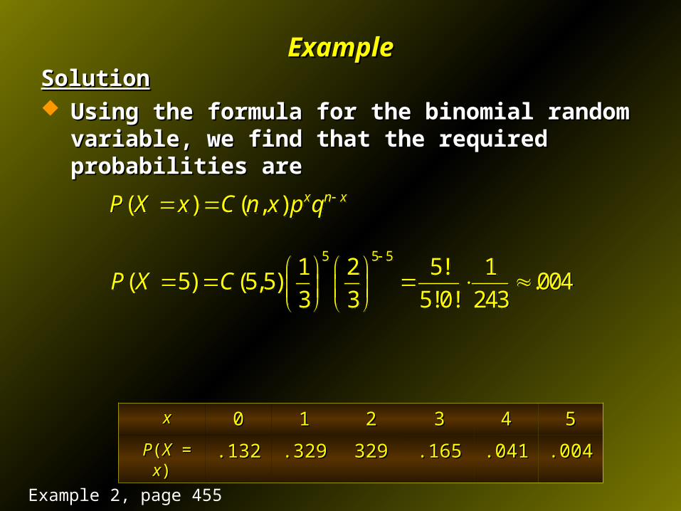
ExampleExampleSolutionSolution Using the formula for the binomial random variable, we Using the formula for the binomial random variable, we
find that the required probabilities arefind that the required probabilities are
( ) ( , ) x n xP X x C n x p q ( ) ( , ) x n xP X x C n x p q
5 5 51 2 5! 1
( 5) (5,5) .0043 3 5!0! 243
P X C
5 5 51 2 5! 1
( 5) (5,5) .0043 3 5!0! 243
P X C
xx 00 11 22 33 44 55
PP((XX = = xx)) .132.132 .329.329 329329 .165.165 .041.041 .004.004
Example 2, page 455
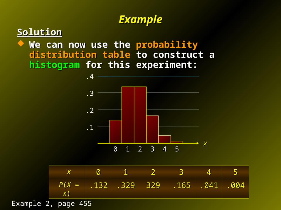
ExampleExampleSolutionSolution We can now use the We can now use the probability distribution tableprobability distribution table to to
construct a construct a histogramhistogram for this experiment: for this experiment:
xx 00 11 22 33 44 55
PP((XX = = xx)) .132.132 .329.329 329329 .165.165 .041.041 .004.004
00 11 22 33 44 55
.4
.3
.2
.1
xx
Example 2, page 455
Applied Example:Applied Example: Quality Control Quality Control
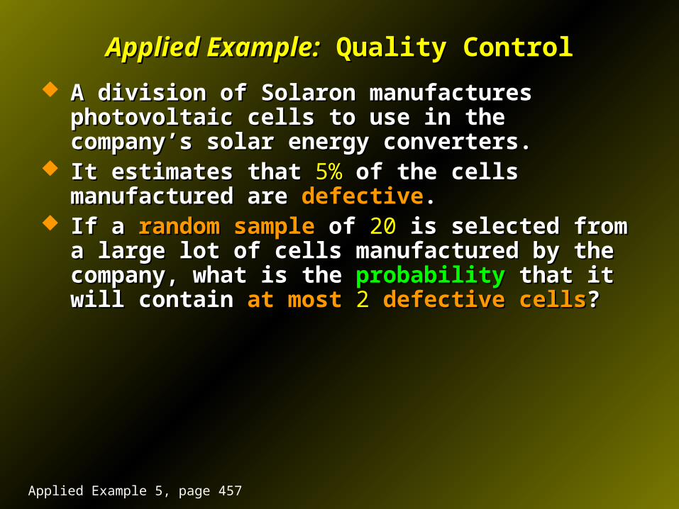
A division of Solaron manufactures photovoltaic cells to A division of Solaron manufactures photovoltaic cells to use in the company’s solar energy converters.use in the company’s solar energy converters.
It estimates that It estimates that 5%5% of the cells manufactured are of the cells manufactured are defectivedefective..
If a If a random samplerandom sample of of 2020 is selected from a large lot of is selected from a large lot of cells manufactured by the company, what is the cells manufactured by the company, what is the probabilityprobability that it will contain that it will contain at mostat most 22 defective cellsdefective cells??
Applied Example 5, page 457
Applied Example:Applied Example: Quality Control Quality Control
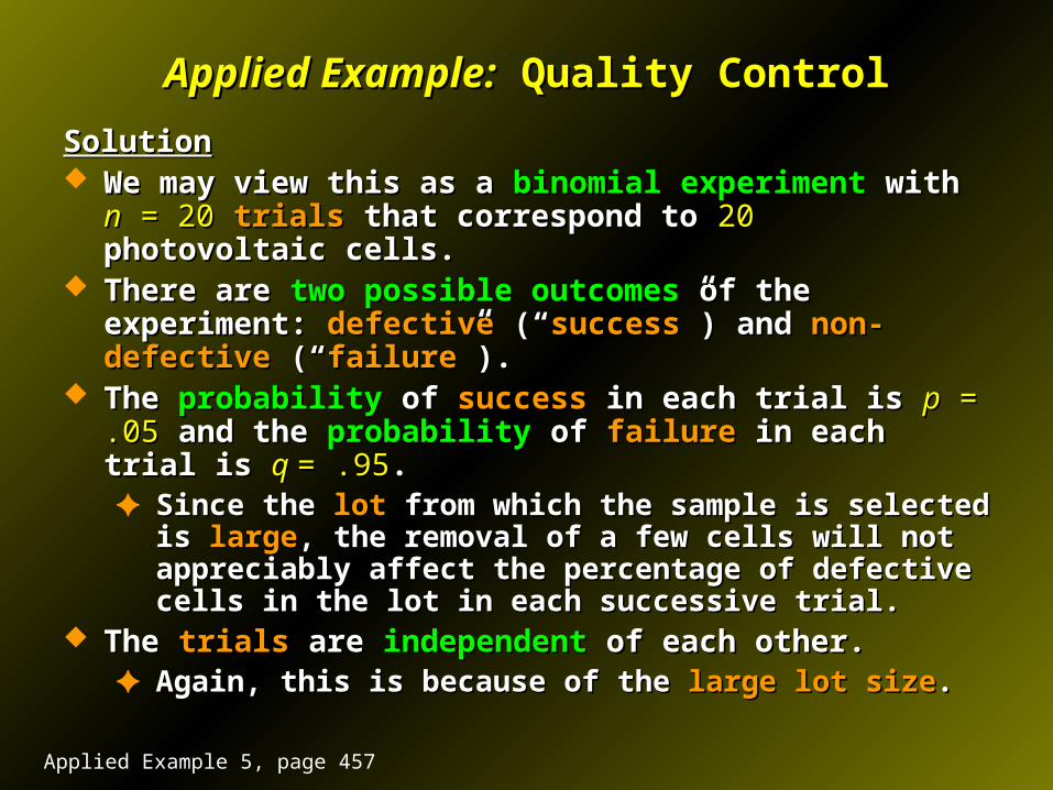
SolutionSolution We may view this as a We may view this as a binomial experimentbinomial experiment with with nn = 20 = 20
trialstrials that correspond to that correspond to 2020 photovoltaic cells. photovoltaic cells. There are There are two possible outcomestwo possible outcomes of the experiment: of the experiment:
defectivedefective (“ (“successsuccess”) and ”) and non-defectivenon-defective (“ (“failurefailure”).”). The The probability probability ofof successsuccess in each trial is in each trial is pp = .05 = .05 and the and the
probability probability ofof failurefailure in each trial is in each trial is q q = .95= .95..✦ Since the Since the lotlot from which the sample is selected is from which the sample is selected is largelarge, ,
the removal of a few cells will not appreciably affect the the removal of a few cells will not appreciably affect the percentage of defective cells in the lot in each successive percentage of defective cells in the lot in each successive trial.trial.
The The trialstrials are are independentindependent of each other. of each other.✦ Again, this is because of the Again, this is because of the large lot sizelarge lot size..
Applied Example 5, page 457
Applied Example:Applied Example: Quality Control Quality Control
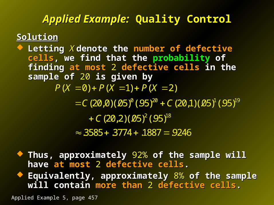
SolutionSolution Letting Letting X X denote the denote the number of defective cellsnumber of defective cells, we find , we find
that the that the probabilityprobability of finding of finding at mostat most 22 defective cellsdefective cells in in the sample of the sample of 2020 is given by is given by
Thus, approximately Thus, approximately 92%92% of the sample will have of the sample will have at mostat most 22 defective cellsdefective cells..
Equivalently, approximately Equivalently, approximately 8%8% of the sample will contain of the sample will contain more thanmore than 22 defective cellsdefective cells..
0 20 1 19
2 18
( 0) ( 1) ( 2)
(20,0)(.05) (.95) (20,1)(.05) (.95)
(20,2)(.05) (.95)
.3585 .3774 .1887 .9246
P X P X P X
C C
C
0 20 1 19
2 18
( 0) ( 1) ( 2)
(20,0)(.05) (.95) (20,1)(.05) (.95)
(20,2)(.05) (.95)
.3585 .3774 .1887 .9246
P X P X P X
C C
C
Applied Example 5, page 457
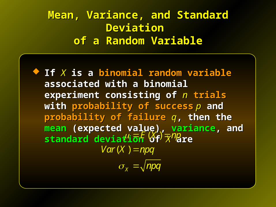
If If XX is a is a binomial random variablebinomial random variable associated with associated with a binomial experiment consisting of a binomial experiment consisting of nn trialstrials with with probability of successprobability of success p p and and probability of failureprobability of failure qq, then the , then the meanmean (expected value), (expected value), variancevariance, and , and standard deviationstandard deviation of of XX are are
Mean, Variance, and Standard Deviation Mean, Variance, and Standard Deviation of a Random Variableof a Random Variable
( )
( )
X
E X np
Var X npq
npq
( )
( )
X
E X np
Var X npq
npq
Applied Example:Applied Example: Quality Control Quality Control
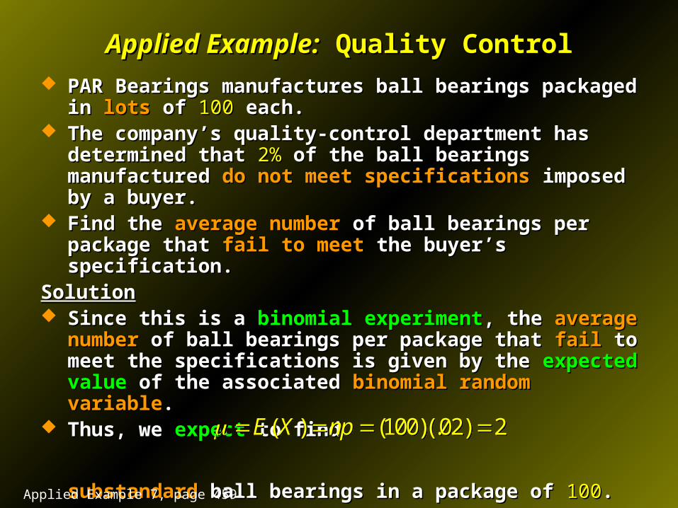
PAR Bearings manufactures ball bearings packaged in PAR Bearings manufactures ball bearings packaged in lotslots of of 100100 each. each.
The company’s quality-control department has determined The company’s quality-control department has determined that that 2%2% of the ball bearings manufactured of the ball bearings manufactured do not meet do not meet specificationsspecifications imposed by a buyer. imposed by a buyer.
Find the Find the average numberaverage number of ball bearings per package that of ball bearings per package that fail to meetfail to meet the buyer’s specification. the buyer’s specification.
SolutionSolution Since this is a Since this is a binomial experimentbinomial experiment, the , the average numberaverage number of of
ball bearings per package that ball bearings per package that failfail to meet the specifications to meet the specifications is given by the is given by the expected valueexpected value of the associated of the associated binomial binomial random variablerandom variable. .
Thus, we Thus, we expectexpect to find to find
substandardsubstandard ball bearings in a package of ball bearings in a package of 100100..
( ) (100)(.02) 2E X np ( ) (100)(.02) 2E X np
Applied Example 7, page 459
8.58.5The Normal DistributionThe Normal Distribution
x
y
( )y f x ( )y f x
Area is
.9545
– 2 + 2
Probability Density FunctionsProbability Density Functions
In this section we consider probability distributions In this section we consider probability distributions associated with a associated with a continuous random variablecontinuous random variable: : ✦ A random variable that may take on A random variable that may take on any valueany value lying in lying in
an interval of an interval of real numbersreal numbers.. Such probability distributions are called Such probability distributions are called continuous continuous
probability distributionsprobability distributions.. A continuous probability distribution is defined by a A continuous probability distribution is defined by a
functionfunction ff whose whose domaindomain coincides with the interval of coincides with the interval of values taken on by the values taken on by the random variablerandom variable associated with associated with the the experimentexperiment..
Such a Such a functionfunction ff is called the is called the probability density functionprobability density function associated with the probability distribution.associated with the probability distribution.
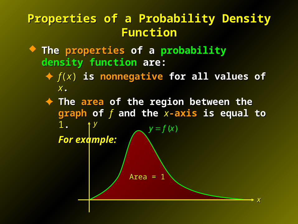
Properties of a Probability Density FunctionProperties of a Probability Density Function
The The propertiesproperties of a of a probability density functionprobability density function are: are:✦ ff((xx)) is is nonnegativenonnegative for all values of for all values of xx..
✦ The The areaarea of the region between the of the region between the graphgraph of of ff and and the the xx-axis-axis is equal to is equal to 11. .
For example:For example:
xx
yy( )y f x ( )y f x
Area = 1Area = 1
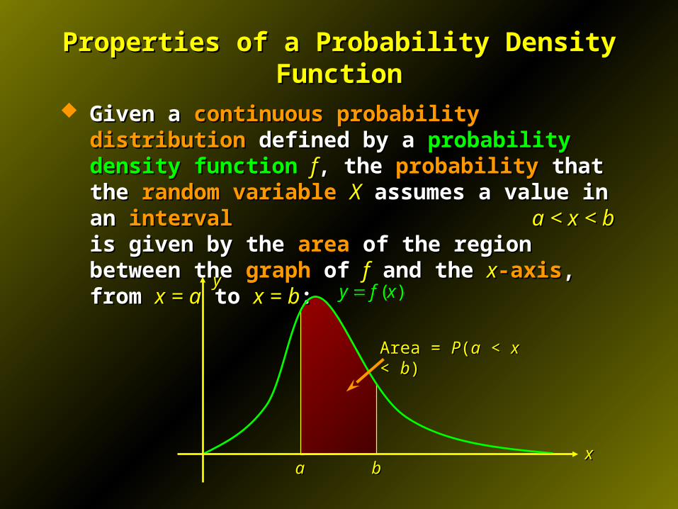
Properties of a Probability Density FunctionProperties of a Probability Density Function
Given a Given a continuous probability distributioncontinuous probability distribution defined by a defined by a probability density functionprobability density function ff, the , the probabilityprobability that the that the random variablerandom variable XX assumes a value in an assumes a value in an intervalinterval a < x < ba < x < b is given by the is given by the areaarea of the region between of the region between the the graphgraph of of ff and the and the xx-axis-axis, from , from x = ax = a to to x = bx = b::
xx
yy
Area = Area = PP((aa < < xx < < bb))
aa bb
( )y f x ( )y f x
Properties of a Probability Density FunctionProperties of a Probability Density Function
The The meanmean and the and the standard deviationstandard deviation of a of a continuouscontinuous probability distribution have probability distribution have roughly the same meaningroughly the same meaning as as the mean and standard deviation of a the mean and standard deviation of a finitefinite probability probability distribution.distribution.
The The meanmean of a of a continuouscontinuous probability distribution is a probability distribution is a measure of the measure of the central tendencycentral tendency of the probability of the probability distribution, and the distribution, and the standard deviationstandard deviation measures its measures its spread about the meanspread about the mean..
Normal DistributionsNormal Distributions
A A special classspecial class of continuous probability distributions is of continuous probability distributions is known as known as normal distributionsnormal distributions..
The The normal distributionsnormal distributions are without doubt the are without doubt the most most importantimportant of all the probability distributions. of all the probability distributions.
There are There are many phenomenamany phenomena with probability with probability distributions that are approximately distributions that are approximately normalnormal::✦ For example, the heights of people, the weights of For example, the heights of people, the weights of
newborn infants, the IQs of college students, the actual newborn infants, the IQs of college students, the actual weights of 16-ounce packages of cereal, and so on.weights of 16-ounce packages of cereal, and so on.
The The normal distributionnormal distribution also provides us with an also provides us with an accurate approximation to the distributions of many accurate approximation to the distributions of many random variablesrandom variables associated with associated with random-samplingrandom-sampling problems.problems.
Normal DistributionsNormal Distributions
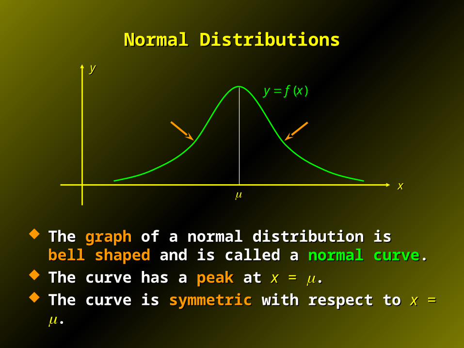
The The graphgraph of a normal distribution is of a normal distribution is bell shapedbell shaped and is and is called a called a normal curvenormal curve..
The curve has a The curve has a peakpeak at at xx = = .. The curve is The curve is symmetricsymmetric with respect to with respect to xx = = ..
xx
yy
( )y f x ( )y f x
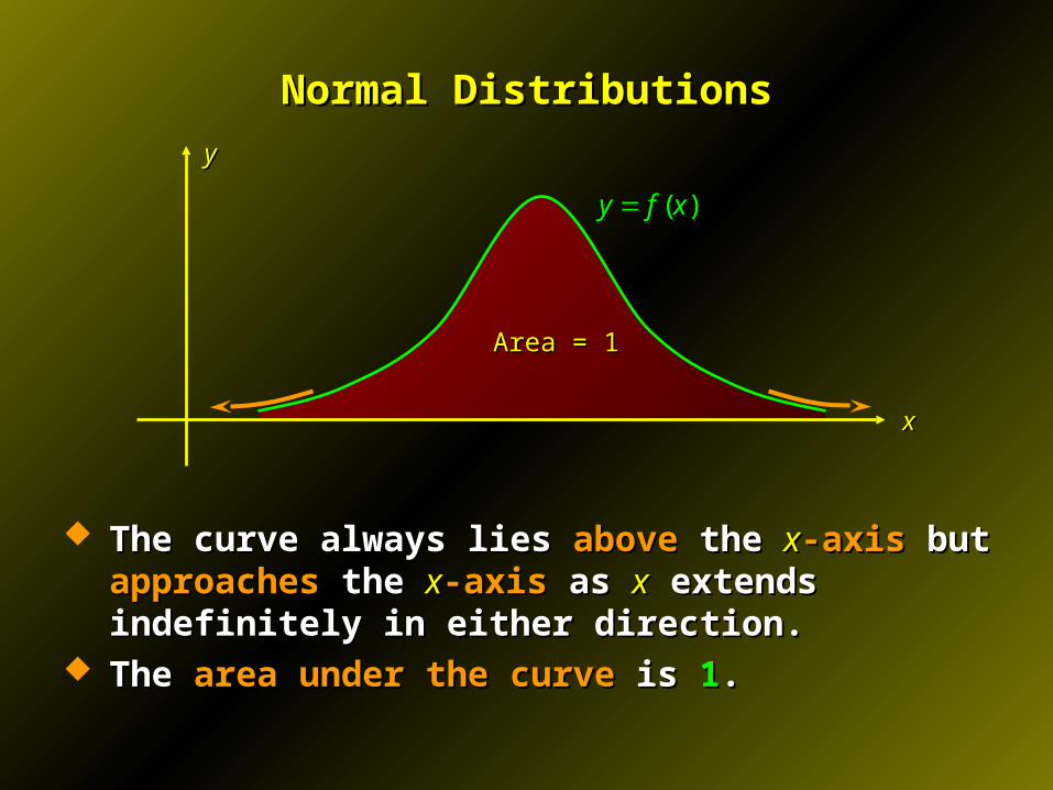
Normal DistributionsNormal Distributions
The curve always lies The curve always lies aboveabove the the xx-axis-axis but but approachesapproaches the the xx-axis-axis as as xx extends indefinitely in either direction. extends indefinitely in either direction.
The The area under the curvearea under the curve is is 11..
xx
yy
( )y f x ( )y f x
Area = 1Area = 1
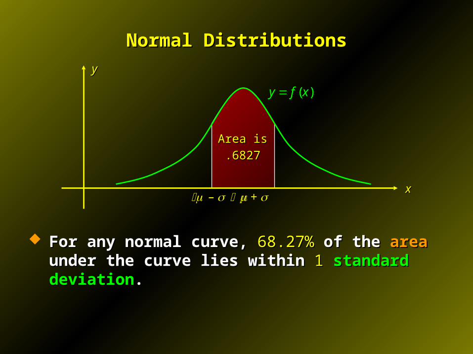
Normal DistributionsNormal Distributions
For any normal curve, For any normal curve, 68.27%68.27% of the of the areaarea under the under the curve lies within curve lies within 11 standard deviationstandard deviation..
xx
yy
( )y f x ( )y f x
Area isArea is
.6827.6827
– – + +
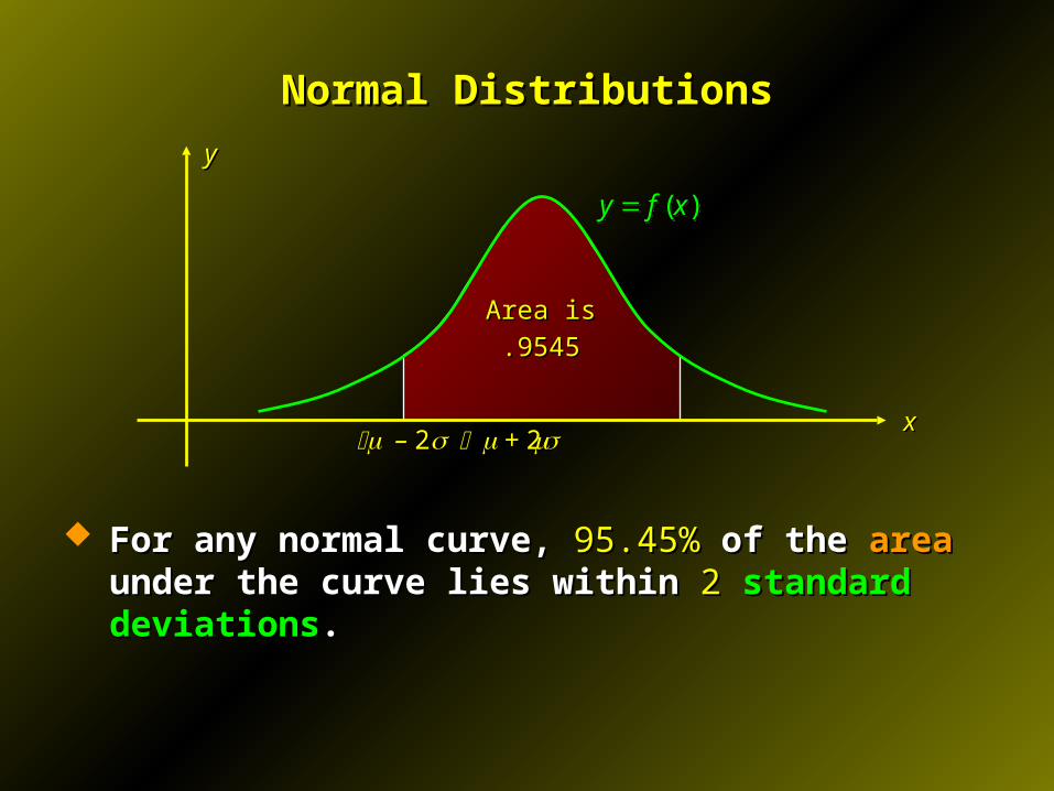
Normal DistributionsNormal Distributions
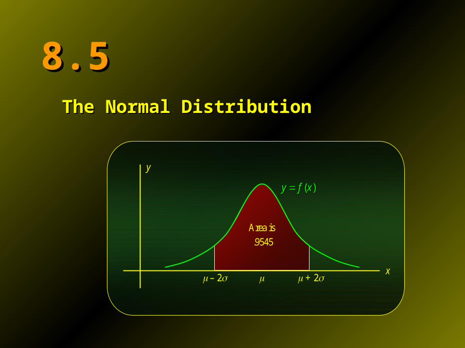
For any normal curve, For any normal curve, 95.45%95.45% of the of the areaarea under the under the curve lies within curve lies within 22 standard deviationsstandard deviations..
xx
yy
( )y f x ( )y f x
Area isArea is
.9545.9545
– – 22 + + 22
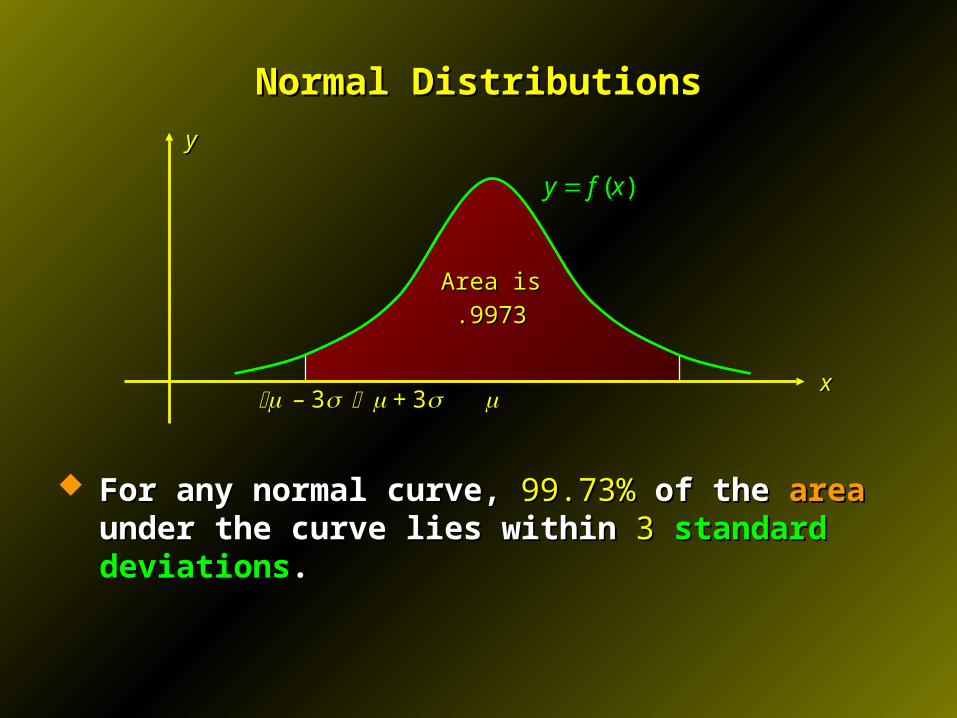
Normal DistributionsNormal Distributions
For any normal curve, For any normal curve, 99.73%99.73% of the of the areaarea under the under the curve lies within curve lies within 33 standard deviationsstandard deviations..
xx
yy
( )y f x ( )y f x
Area isArea is
.9973.9973
– – 33 + + 33
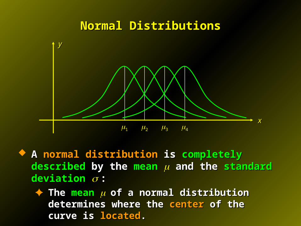
Normal DistributionsNormal Distributions
A A normal distributionnormal distribution is is completely describedcompletely described by the by the meanmean and the and the standard deviation standard deviation ::✦ The The meanmean of a normal distribution determines where of a normal distribution determines where
the the centercenter of the curve is of the curve is locatedlocated..
xx
yy
11 22 33 44
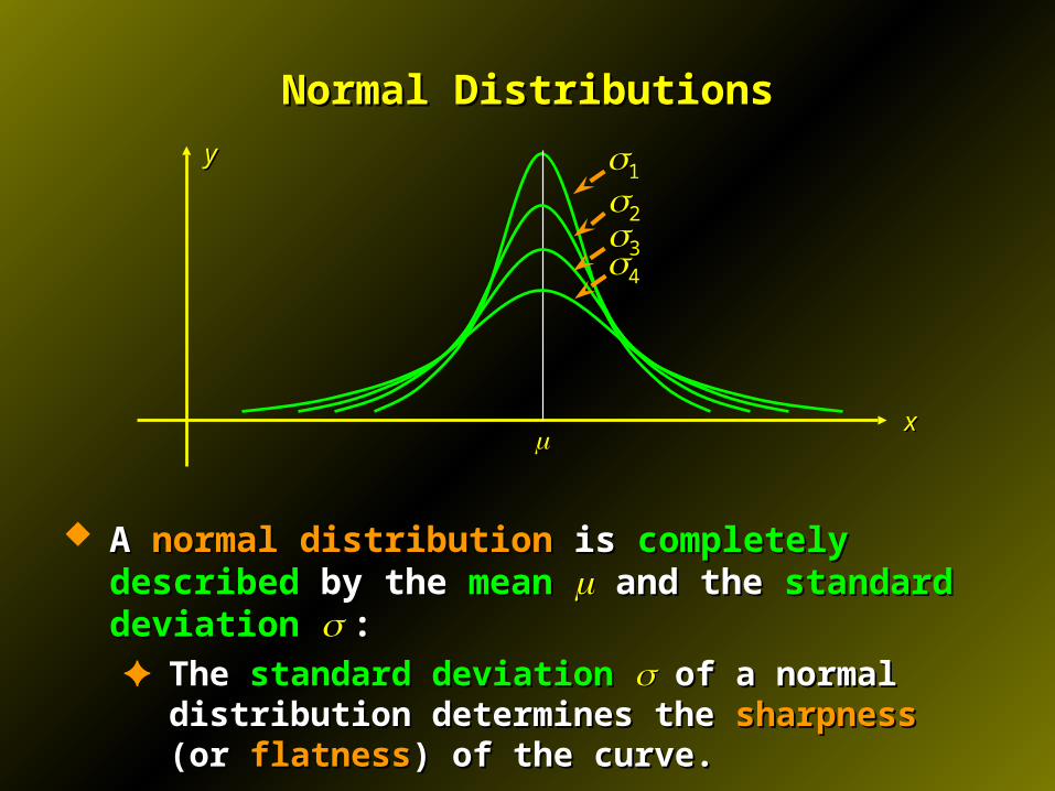
Normal DistributionsNormal Distributions
A A normal distributionnormal distribution is is completely describedcompletely described by the by the meanmean and the and the standard deviation standard deviation ::✦ The The standard deviationstandard deviation of a normal distribution of a normal distribution
determines the determines the sharpnesssharpness (or (or flatnessflatness) of the curve.) of the curve.
xx
yy
11
223344
Normal DistributionsNormal Distributions
There are infinitely There are infinitely many normal curvesmany normal curves corresponding corresponding to different to different meansmeans and and standard deviations standard deviations ..
Fortunately, Fortunately, any normal curveany normal curve may be may be transformedtransformed into into any other normal curveany other normal curve, so in the study of normal curves , so in the study of normal curves it is enough to single out one such particular curve for it is enough to single out one such particular curve for special attention.special attention.
The normal curve with The normal curve with meanmean = 0= 0 and and standard standard deviation deviation = 1= 1 is called the is called the standard normal curvestandard normal curve..
The corresponding distribution is called the The corresponding distribution is called the standard standard normal distributionnormal distribution..
The random variable itself is called the The random variable itself is called the standard normal standard normal variablevariable and is commonly denoted by and is commonly denoted by ZZ..
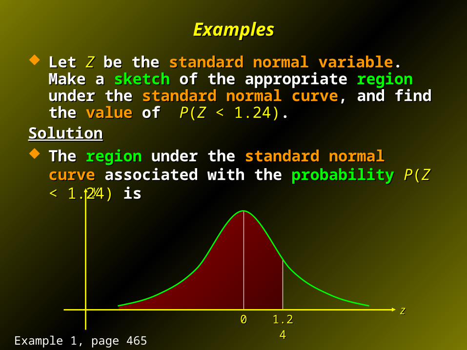
ExamplesExamples
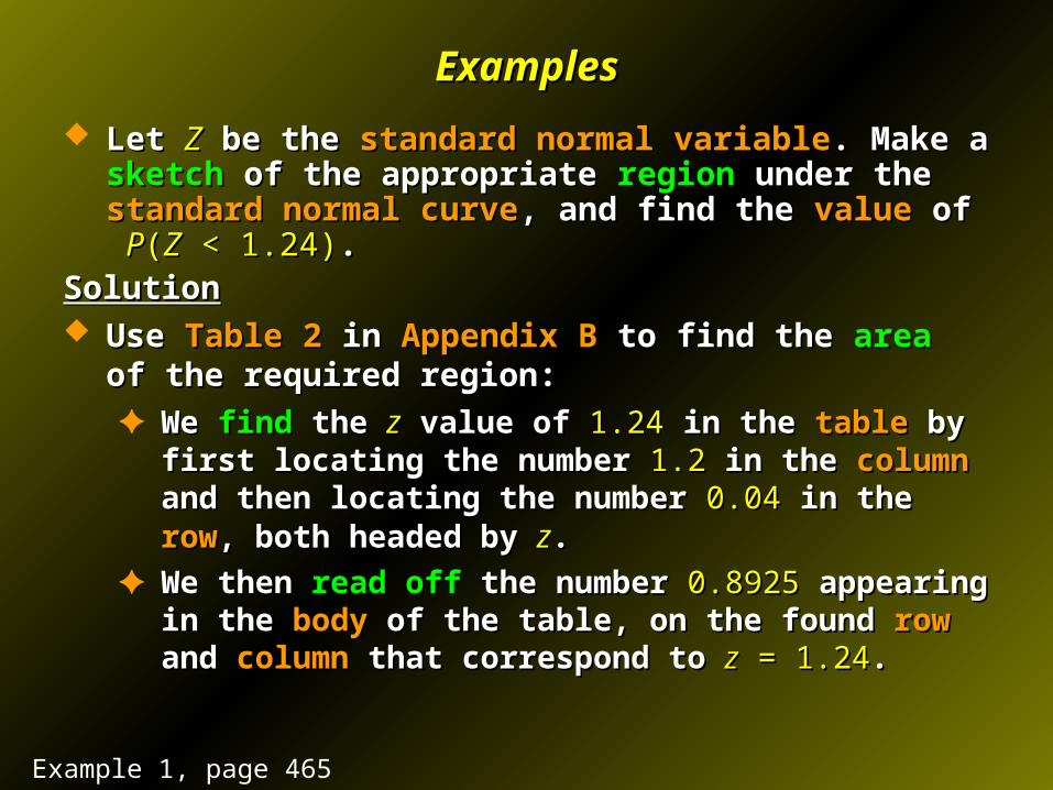
Let Let ZZ be the be the standard normal variablestandard normal variable. Make a . Make a sketchsketch of of the appropriate the appropriate regionregion under the under the standard normal curvestandard normal curve, , and find the and find the valuevalue of of PP((ZZ < 1.24) < 1.24). .
SolutionSolution The The regionregion under the under the standard normal curvestandard normal curve associated associated
with the with the probabilityprobability PP((ZZ < 1.24) < 1.24) is is
zz
yy
1.241.2400
Example 1, page 465
ExamplesExamples
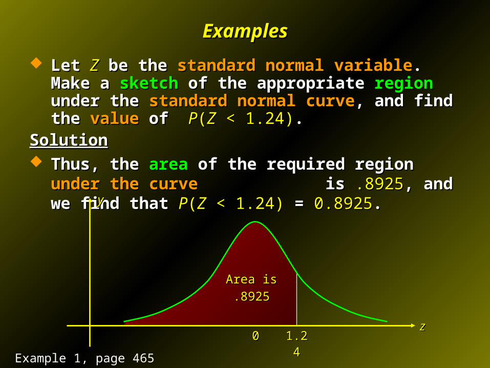
Let Let ZZ be the be the standard normal variablestandard normal variable. Make a . Make a sketchsketch of of the appropriate the appropriate regionregion under the under the standard normal curvestandard normal curve, , and find the and find the valuevalue of of PP((ZZ < 1.24) < 1.24). .
SolutionSolution Use Use Table 2Table 2 in in Appendix BAppendix B to find the to find the areaarea of the required of the required
region:region:✦ We We findfind the the zz value of value of 1.241.24 in the in the tabletable by first locating by first locating
the number the number 1.21.2 in the in the columncolumn and then locating the and then locating the number number 0.040.04 in the in the rowrow, both headed by , both headed by zz..
✦ We then We then read offread off the number the number 0.8925 0.8925 appearing in the appearing in the bodybody of the table, on the found of the table, on the found rowrow and and columncolumn that that correspond to correspond to zz = 1.24 = 1.24..
Example 1, page 465
ExamplesExamples
Let Let ZZ be the be the standard normal variablestandard normal variable. Make a . Make a sketchsketch of of the appropriate the appropriate regionregion under the under the standard normal curvestandard normal curve, , and find the and find the valuevalue of of PP((ZZ < 1.24) < 1.24). .
SolutionSolution Thus, the Thus, the areaarea of the required region of the required region under the curveunder the curve
is is .8925.8925, and we find that , and we find that PP((ZZ < 1.24) < 1.24) = = 0.8925 0.8925..
zz
yy
Area isArea is
.8925.8925
1.241.2400
Example 1, page 465
ExamplesExamples
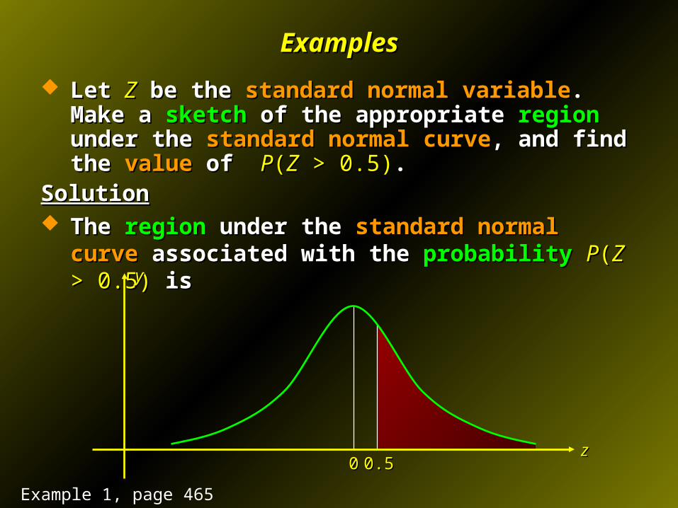
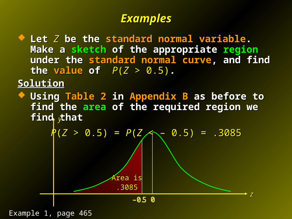
Let Let ZZ be the be the standard normal variablestandard normal variable. Make a . Make a sketchsketch of of the appropriate the appropriate regionregion under the under the standard normal curvestandard normal curve, , and find the and find the valuevalue of of PP((ZZ > 0.5) > 0.5). .
SolutionSolution The The regionregion under the under the standard normal curvestandard normal curve associated associated
with the with the probabilityprobability PP((ZZ > 0.5) > 0.5) is is
zz
yy
0.50.500
Example 1, page 465
00–– 0.50.5
ExamplesExamples
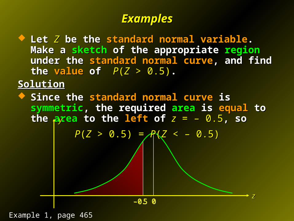
Let Let ZZ be the be the standard normal variablestandard normal variable. Make a . Make a sketchsketch of of the appropriate the appropriate regionregion under the under the standard normal curvestandard normal curve, , and find the and find the valuevalue of of PP((ZZ > 0.5) > 0.5). .
SolutionSolution Since the Since the standard normal curvestandard normal curve is is symmetricsymmetric, the , the
required required areaarea is is equalequal to the to the areaarea to the to the leftleft of of zz = – 0.5 = – 0.5, so, so
PP((ZZ > 0.5) > 0.5) = = PP((ZZ < – 0.5) < – 0.5)
zz
yy
Example 1, page 465
00–– 0.50.5
ExamplesExamples
Let Let ZZ be the be the standard normal variablestandard normal variable. Make a . Make a sketchsketch of of the appropriate the appropriate regionregion under the under the standard normal curvestandard normal curve, , and find the and find the valuevalue of of PP((ZZ > 0.5) > 0.5). .
SolutionSolution Using Using Table 2Table 2 in in Appendix BAppendix B as before to find the as before to find the areaarea of of
the required region we find thatthe required region we find that
PP((ZZ > 0.5) > 0.5) = = PP((ZZ < – 0.5) = .3085 < – 0.5) = .3085
zz
yy
Area isArea is.3085.3085
Example 1, page 465
ExamplesExamples
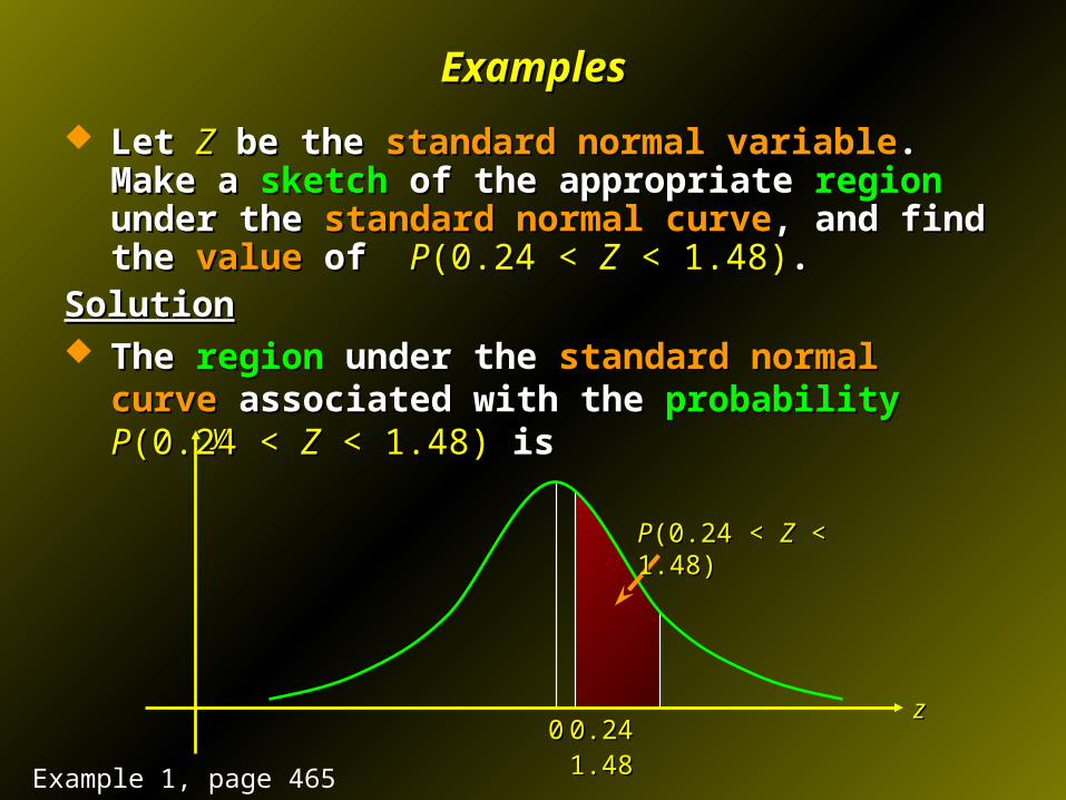
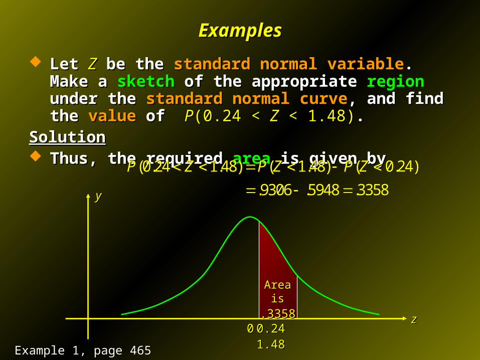
Let Let ZZ be the be the standard normal variablestandard normal variable. Make a . Make a sketchsketch of of the appropriate the appropriate regionregion under the under the standard normal curvestandard normal curve, , and find the and find the valuevalue of of PP(0.24 < (0.24 < ZZ < 1.48) < 1.48). .
SolutionSolution The The regionregion under the under the standard normal curvestandard normal curve associated associated
with the with the probabilityprobability PP(0.24 < (0.24 < ZZ < 1.48) < 1.48) is is
zz
yy
0.24 1.480.24 1.4800
PP(0.24 < (0.24 < ZZ < 1.48) < 1.48)
Example 1, page 465
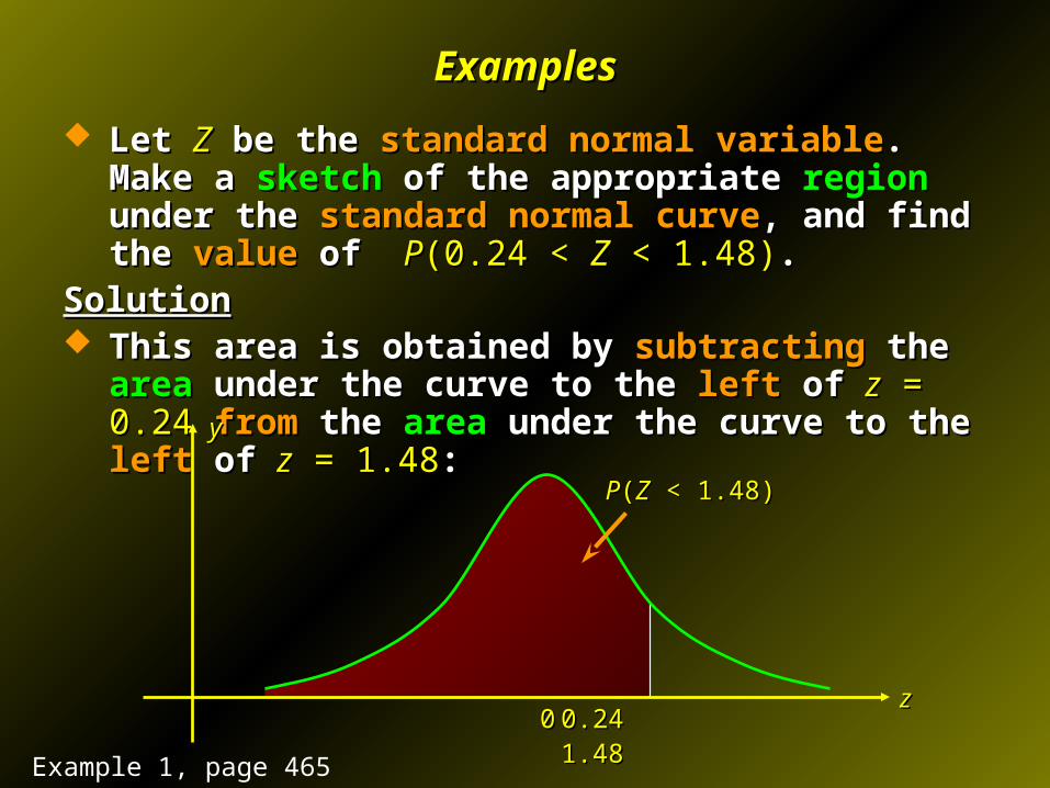
ExamplesExamples
Let Let ZZ be the be the standard normal variablestandard normal variable. Make a . Make a sketchsketch of of the appropriate the appropriate regionregion under the under the standard normal curvestandard normal curve, , and find the and find the valuevalue of of PP(0.24 < (0.24 < ZZ < 1.48) < 1.48). .
SolutionSolution This area is obtained by This area is obtained by subtractingsubtracting the the areaarea under the under the
curve to the curve to the leftleft of of zz = 0.24 = 0.24 fromfrom the the areaarea under the curve under the curve to the to the leftleft of of zz = 1.48 = 1.48::
zz
yy
00
PP((ZZ < 1.48) < 1.48)
0.24 1.480.24 1.48
Example 1, page 465
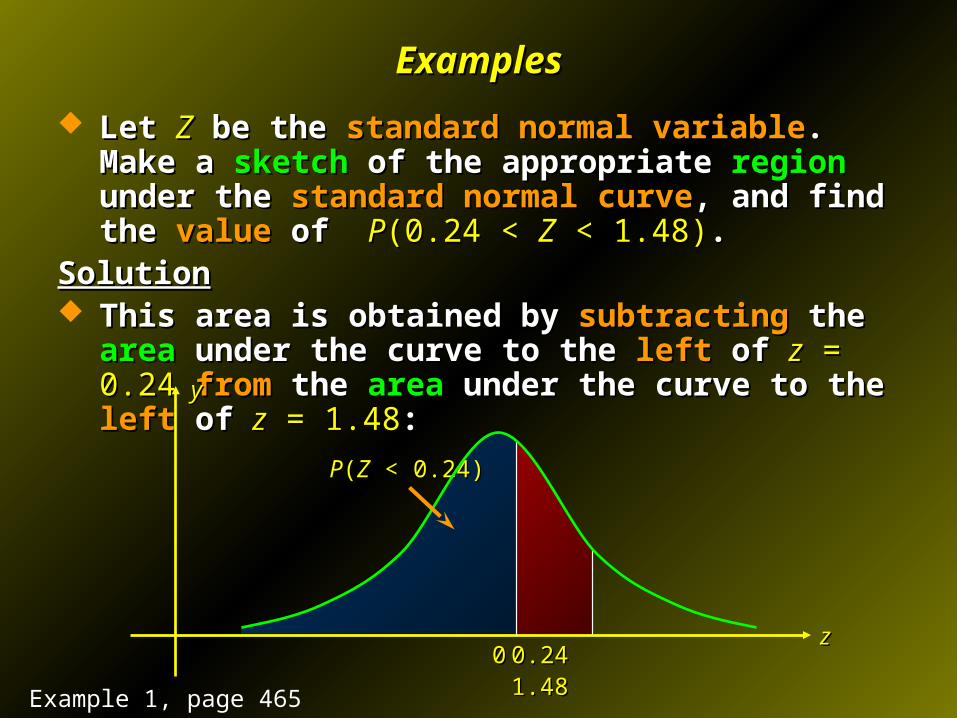
ExamplesExamples
Let Let ZZ be the be the standard normal variablestandard normal variable. Make a . Make a sketchsketch of of the appropriate the appropriate regionregion under the under the standard normal curvestandard normal curve, , and find the and find the valuevalue of of PP(0.24 < (0.24 < ZZ < 1.48) < 1.48). .
SolutionSolution This area is obtained by This area is obtained by subtractingsubtracting the the areaarea under the under the
curve to the curve to the leftleft of of zz = 0.24 = 0.24 fromfrom the the areaarea under the curve under the curve to the to the leftleft of of zz = 1.48 = 1.48::
zz
yy
0.24 1.480.24 1.4800
PP((ZZ < 0.24) < 0.24)
Example 1, page 465
ExamplesExamples
Let Let ZZ be the be the standard normal variablestandard normal variable. Make a . Make a sketchsketch of of the appropriate the appropriate regionregion under the under the standard normal curvestandard normal curve, , and find the and find the valuevalue of of PP(0.24 < (0.24 < ZZ < 1.48) < 1.48). .
SolutionSolution Thus, the required Thus, the required areaarea is given by is given by
zz
yy
0.24 1.480.24 1.4800
(0.24 1.48) ( 1.48) ( 0.24)
.9306 .5948 .3358
P Z P Z P Z
(0.24 1.48) ( 1.48) ( 0.24)
.9306 .5948 .3358
P Z P Z P Z
Area isArea is
.3358.3358
Example 1, page 465

Transforming into a Standard Normal CurveTransforming into a Standard Normal Curve
When dealing with a When dealing with a non-standard normal curvenon-standard normal curve, it is , it is possible to possible to transformtransform such a curve into a such a curve into a standard standard normal curvenormal curve..
XZ
X
Z
If If XX is a normal random variable with is a normal random variable with meanmean and and standard deviationstandard deviation , then it can be , then it can be transformedtransformed into the standard normal into the standard normal random variable random variable ZZ by substituting in by substituting in

The The areaarea of the region under the of the region under the normal curvenormal curve between between x x == a a and and x x == b b is equal to the is equal to the areaarea of the of the region under the region under the standard normal curvestandard normal curve between between
Thus, in terms of Thus, in terms of probabilitiesprobabilities we have we have
a bz z
and a b
z z
and
( )a b
P a X b P Z
( )
a bP a X b P Z
Transforming into a Standard Normal CurveTransforming into a Standard Normal Curve
Transforming into a Standard Normal CurveTransforming into a Standard Normal Curve
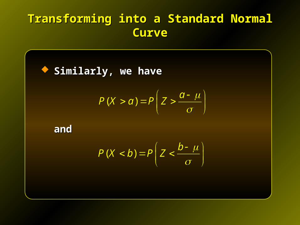
Similarly, we haveSimilarly, we have
andand
( )b
P X b P Z
( )
bP X b P Z
( )a
P X a P Z
( )
aP X a P Z

Transforming into a Standard Normal CurveTransforming into a Standard Normal Curve
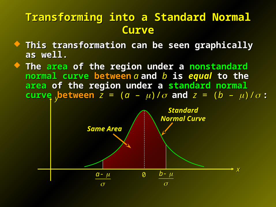
This transformation can be seen graphically as well.This transformation can be seen graphically as well. The The areaarea of the region under a of the region under a nonstandard normal curvenonstandard normal curve
betweenbetween a a and and bb is is equalequal to the to the areaarea of the region under a of the region under a standard normal curvestandard normal curve betweenbetween zz = ( = (aa – – )/)/ and and zz = ( = (bb – – )/)/::
xx
yy
aa bb
Nonstandard Nonstandard Normal CurveNormal Curve
Same AreaSame Area
Transforming into a Standard Normal CurveTransforming into a Standard Normal Curve
xx
yy
00a a b
b
This transformation can be seen graphically as well.This transformation can be seen graphically as well. The The areaarea of the region under a of the region under a nonstandard normal curvenonstandard normal curve
betweenbetween a a and and bb is is equalequal to the to the areaarea of the region under a of the region under a standard normal curvestandard normal curve betweenbetween zz = ( = (aa – – )/)/ and and zz = ( = (bb – – )/)/::
Standard Standard Normal CurveNormal Curve
Same AreaSame Area
ExampleExample
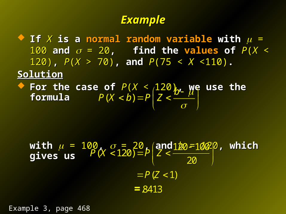
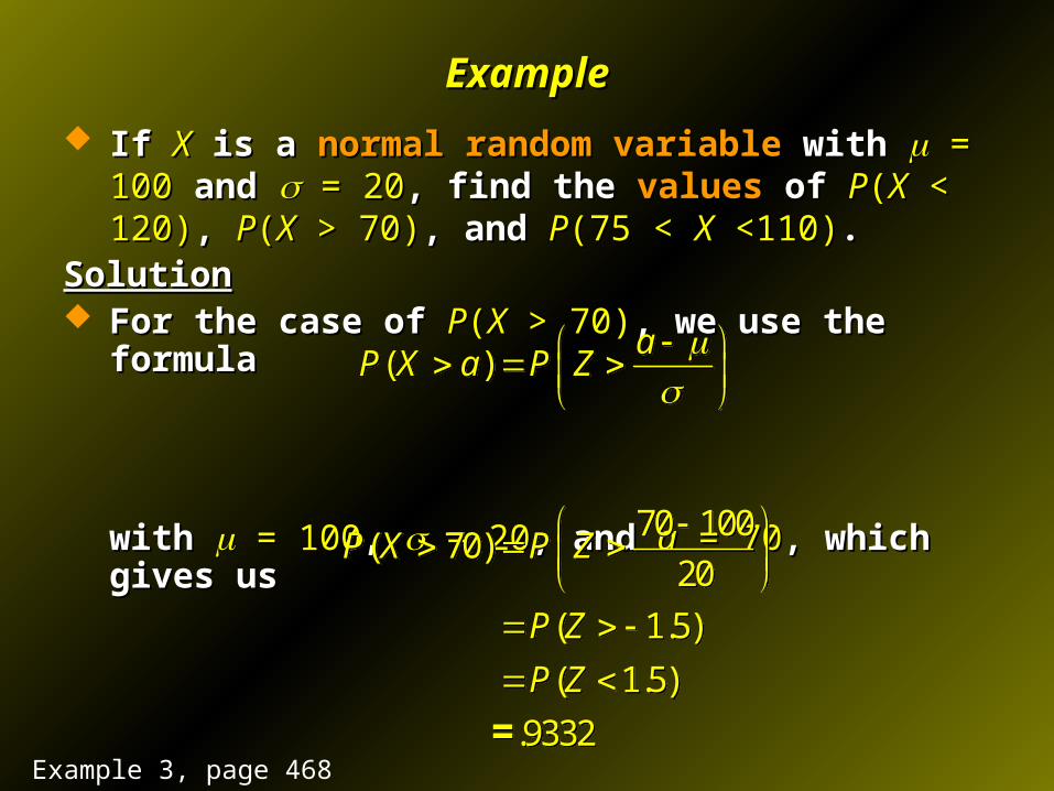
If If XX is a is a normal random variablenormal random variable with with = 100= 100 and and = 20 = 20, , find the find the valuesvalues of of PP((XX < 120) < 120), , PP((XX > 70) > 70), and , and PP(75 < (75 < XX <110) <110). .
SolutionSolution For the case of For the case of PP((XX < 120) < 120), we use the formula, we use the formula
with with = 100= 100, , = 20 = 20, and , and bb = 120 = 120, which gives us, which gives us
( )b
P X b P Z
( )
bP X b P Z
120 100( 120)
20
( 1)
.8413
P X P Z
P Z
=
120 100( 120)
20
( 1)
.8413
P X P Z
P Z
=
Example 3, page 468
ExampleExample
If If XX is a is a normal random variablenormal random variable with with = 100= 100 and and = 20 = 20, , find the find the valuesvalues of of PP((XX < 120) < 120), , PP((XX > 70) > 70), and , and PP(75 < (75 < XX <110) <110). .
SolutionSolution For the case of For the case of PP((XX > 70) > 70), we use the formula, we use the formula
with with = 100= 100, , = 20 = 20, and , and aa = 70 = 70, which gives us, which gives us
( )a
P X a P Z
( )
aP X a P Z
70 100( 70)
20
( 1.5)
( 1.5)
.9332
P X P Z
P Z
P Z
=
70 100( 70)
20
( 1.5)
( 1.5)
.9332
P X P Z
P Z
P Z
=
Example 3, page 468
ExampleExample
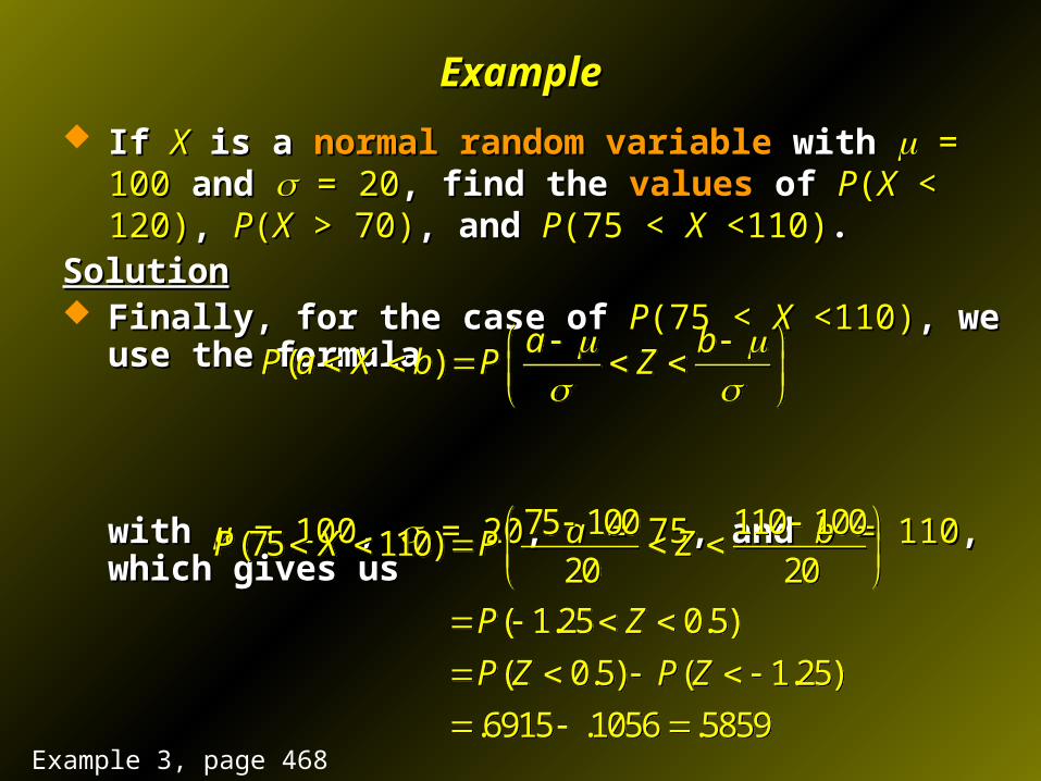
If If XX is a is a normal random variablenormal random variable with with = 100= 100 and and = 20 = 20, , find the find the valuesvalues of of PP((XX < 120) < 120), , PP((XX > 70) > 70), and , and PP(75 < (75 < XX <110) <110). .
SolutionSolution Finally, for the case of Finally, for the case of PP(75 < (75 < XX <110) <110), we use the formula, we use the formula
with with = 100= 100, , = 20 = 20, , aa = 75 = 75, and , and bb = 110 = 110, which gives us, which gives us
( )a b
P a X b P Z
( )
a bP a X b P Z
75 100 110 100(75 110)
20 20
( 1.25 0.5)
( 0.5) ( 1.25)
.6915 .1056 .5859
P X P Z
P Z
P Z P Z
75 100 110 100(75 110)
20 20
( 1.25 0.5)
( 0.5) ( 1.25)
.6915 .1056 .5859
P X P Z
P Z
P Z P Z
Example 3, page 468
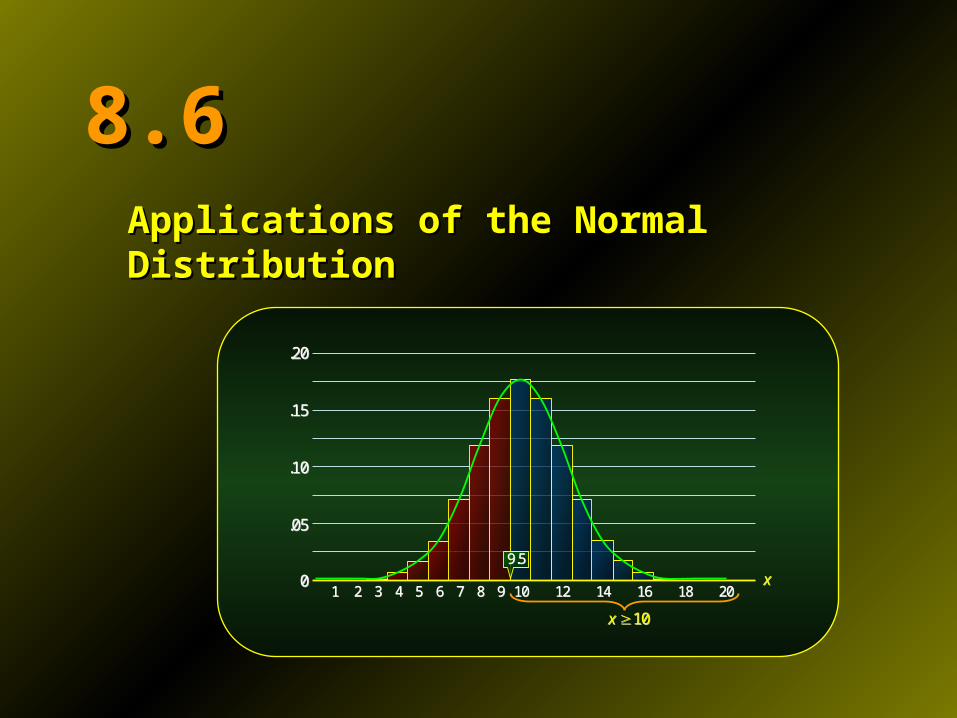
8.68.6Applications of the Normal DistributionApplications of the Normal Distribution
.20.20
.15.15
.10.10
.05.05
0011 22 33 44 55 66 77 88 99 1010 1212 1414 1616 1818 2020
xx
xx 1010
9.59.5
Applied Example:Applied Example: Birth Weights of Infants Birth Weights of Infants
The medical records of infants delivered at the Kaiser The medical records of infants delivered at the Kaiser Memorial Hospital show that the infants’ Memorial Hospital show that the infants’ birth weightsbirth weights in in pounds are pounds are normally distributednormally distributed with a with a meanmean of of 7.4 7.4 and a and a standard deviationstandard deviation of of 1.2 1.2..
Find the Find the probabilityprobability that an infant that an infant selected at randomselected at random from among those delivered at the hospital from among those delivered at the hospital weighed more weighed more thanthan 9.29.2 pounds at birth. pounds at birth.
Applied Example 1, page 471
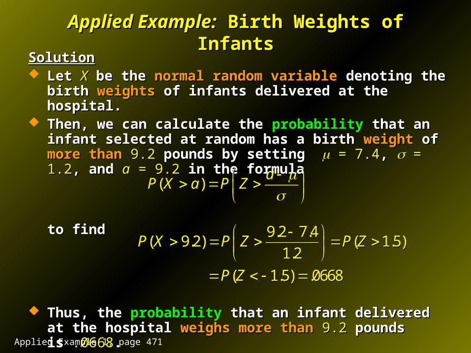
Applied Example:Applied Example: Birth Weights of Infants Birth Weights of InfantsSolutionSolution Let Let XX be the be the normal random variablenormal random variable denoting the birth denoting the birth
weightsweights of infants delivered at the hospital. of infants delivered at the hospital. Then, we can calculate the Then, we can calculate the probabilityprobability that an infant selected that an infant selected
at random has a birth at random has a birth weightweight of of more thanmore than 9.2 9.2 pounds by pounds by setting setting = 7.4 = 7.4, , = 1.2 = 1.2, and , and aa = 9.2 = 9.2 in the formula in the formula
to findto find
Thus, the Thus, the probabilityprobability that an infant delivered at the hospital that an infant delivered at the hospital weighs more thanweighs more than 9.29.2 pounds is pounds is .0668.0668..
( )a
P X a P Z
( )
aP X a P Z
9.2 7.4( 9.2) ( 1.5)
1.2
( 1.5) .0668
P X P Z P Z
P Z
9.2 7.4( 9.2) ( 1.5)
1.2
( 1.5) .0668
P X P Z P Z
P Z
Applied Example 1, page 471
Approximating Binomial DistributionsApproximating Binomial Distributions
One important application of the normal distribution is One important application of the normal distribution is that it can be used to that it can be used to accurately approximateaccurately approximate other other continuous continuous probability distributionsprobability distributions..
As an example, we will see how a As an example, we will see how a binomial distributionbinomial distribution may be may be approximatedapproximated by a suitable by a suitable normal distributionnormal distribution..
This provides a convenient and simple solution to certain This provides a convenient and simple solution to certain problems involving binomial distributions.problems involving binomial distributions.
Approximating Binomial DistributionsApproximating Binomial Distributions
Recall that a Recall that a binomial distributionbinomial distribution is a probability is a probability distribution of the formdistribution of the form
For For small valuessmall values of of nn, the arithmetic computations may be , the arithmetic computations may be done with relative done with relative easeease. However, if . However, if nn is is largelarge, then the , then the work involved becomes work involved becomes overwhelmingoverwhelming, even when tables of , even when tables of PP((X X = = xx)) are available. are available.
( ) ( , ) x n xP X x C n x p q ( ) ( , ) x n xP X x C n x p q
Approximating Binomial DistributionsApproximating Binomial Distributions
To see how a To see how a normal distributionnormal distribution can help in such can help in such situations, consider a situations, consider a coin-tossingcoin-tossing experiment. experiment.
Suppose a fair coin is tossed Suppose a fair coin is tossed 2020 timestimes and we wish to and we wish to compute the compute the probabilityprobability of obtaining of obtaining 1010 or more headsor more heads..
The solution to this problem may be obtained, of course, The solution to this problem may be obtained, of course, by by laboriouslylaboriously computing computing
As an alternative solution, let’s begin by interpreting the As an alternative solution, let’s begin by interpreting the solution in terms of finding the solution in terms of finding the areasareas of rectangles in the of rectangles in the histogramhistogram..
( 10) ( 10) ( 11) ( 20)P X P X P X P X ( 10) ( 10) ( 11) ( 20)P X P X P X P X
Approximating Binomial DistributionsApproximating Binomial Distributions
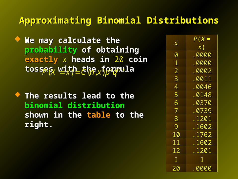
We may calculate the We may calculate the probabilityprobability of of obtaining obtaining exactlyexactly xx heads in heads in 2020 coin coin tosses with the formulatosses with the formula
The results lead to the The results lead to the binomial binomial distributiondistribution shown in the shown in the tabletable to to the right.the right.
( ) ( , ) x n xP X x C n x p q ( ) ( , ) x n xP X x C n x p q
xx PP((X X = = xx))00 .0000.000011 .0000.000022 .0002.000233 .0011.001144 .0046.004655 .0148.014866 .0370.037077 .0739.073988 .1201.120199 .1602.1602
1010 .1762.17621111 .1602.16021212 .1201.1201
2020 .0000.0000
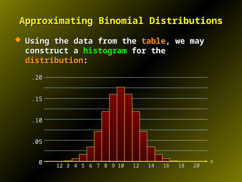
Approximating Binomial DistributionsApproximating Binomial Distributions
Using the data from the Using the data from the tabletable, we may construct a , we may construct a histogramhistogram for the for the distributiondistribution::
.20.20
.15.15
.10.10
.05.05
00 11 22 33 44 55 66 77 88 99 1010 1212 1414 1616 1818 2020
xx
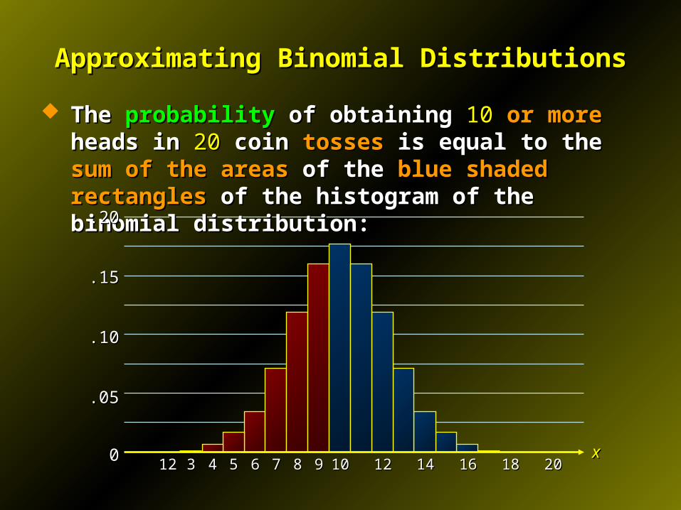
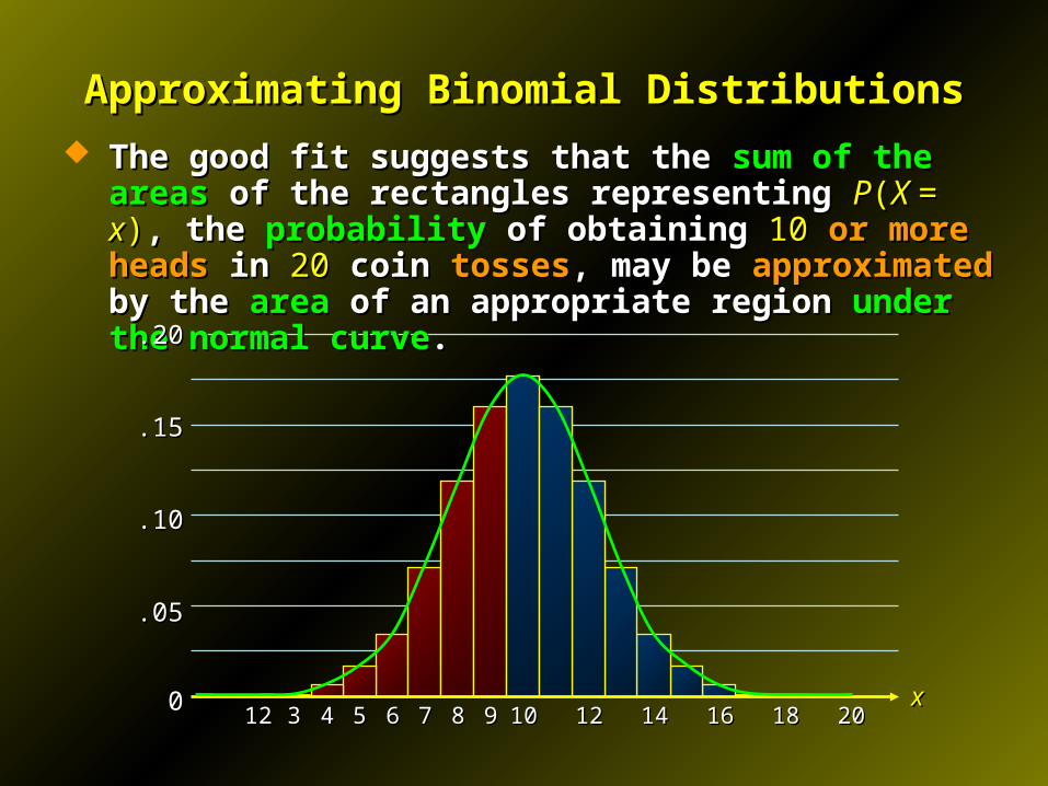
Approximating Binomial DistributionsApproximating Binomial Distributions
The The probabilityprobability of obtaining of obtaining 1010 or moreor more heads in heads in 2020 coin coin tossestosses is equal to the is equal to the sum of the areassum of the areas of the of the blue shaded blue shaded rectanglesrectangles of the histogram of the binomial distribution: of the histogram of the binomial distribution:
.20.20
.15.15
.10.10
.05.05
00 11 22 33 44 55 66 77 88 99 1010 1212 1414 1616 1818 2020
xx
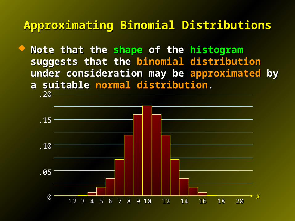
Approximating Binomial DistributionsApproximating Binomial Distributions
Note that the Note that the shapeshape of the of the histogramhistogram suggests that the suggests that the binomial distributionbinomial distribution under consideration may be under consideration may be approximatedapproximated by a suitable by a suitable normal distributionnormal distribution..
.20.20
.15.15
.10.10
.05.05
00 11 22 33 44 55 66 77 88 99 1010 1212 1414 1616 1818 2020
xx
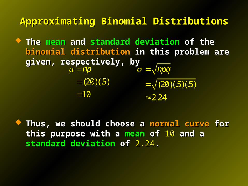
Approximating Binomial DistributionsApproximating Binomial Distributions
The The meanmean and and standard deviationstandard deviation of the of the binomial binomial distributiondistribution in this problem are given, respectively, by in this problem are given, respectively, by
Thus, we should choose a Thus, we should choose a normal curvenormal curve for this purpose for this purpose with a with a meanmean of of 1010 and a and a standard deviationstandard deviation of of 2.242.24..
(20)(.5)
10
np
(20)(.5)
10
np
(20)(.5)(.5)
2.24
npq
(20)(.5)(.5)
2.24
npq
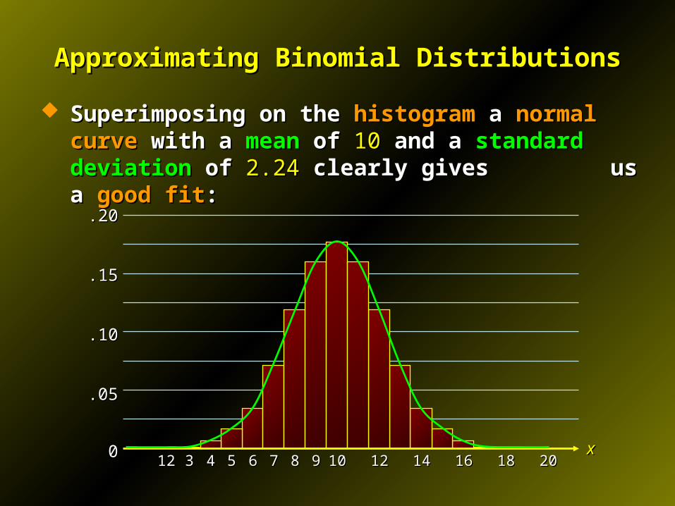
Approximating Binomial DistributionsApproximating Binomial Distributions
Superimposing on the Superimposing on the histogramhistogram a a normal curvenormal curve with a with a meanmean of of 1010 and a and a standard deviationstandard deviation of of 2.24 2.24 clearly gives clearly gives us a us a good fitgood fit::
.20.20
.15.15
.10.10
.05.05
00 11 22 33 44 55 66 77 88 99 1010 1212 1414 1616 1818 2020
xx
Approximating Binomial DistributionsApproximating Binomial Distributions
The good fit suggests that the The good fit suggests that the sum of the areassum of the areas of the of the rectangles representing rectangles representing PP((X X = = xx)), the , the probabilityprobability of obtaining of obtaining 1010 or more headsor more heads in in 2020 coin coin tossestosses, may be , may be approximatedapproximated by by the the areaarea of an appropriate region of an appropriate region under the normal curveunder the normal curve..
.20.20
.15.15
.10.10
.05.05
00 11 22 33 44 55 66 77 88 99 1010 1212 1414 1616 1818 2020
xx
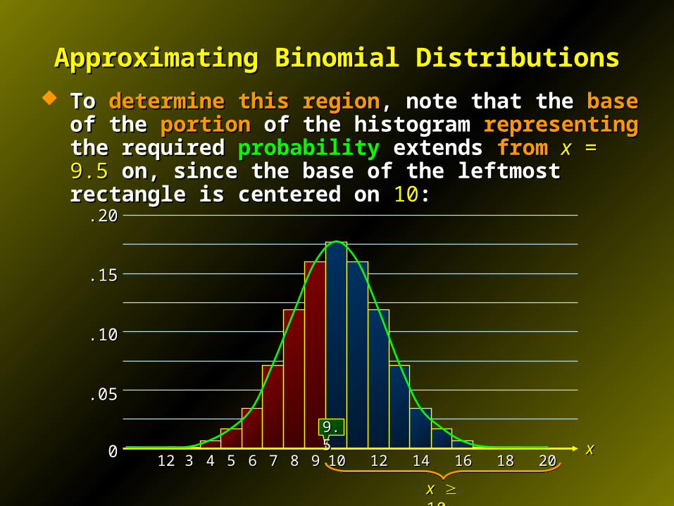
Approximating Binomial DistributionsApproximating Binomial Distributions
To To determine this regiondetermine this region, note that the , note that the basebase of the of the portionportion of of the histogram the histogram representingrepresenting the required the required probabilityprobability extends extends fromfrom xx = 9.5 = 9.5 on, since the base of the leftmost rectangle is on, since the base of the leftmost rectangle is centered on centered on 1010::
.20.20
.15.15
.10.10
.05.05
00 11 22 33 44 55 66 77 88 99 1010 1212 1414 1616 1818 2020
xx
xx 10 10
9.59.5
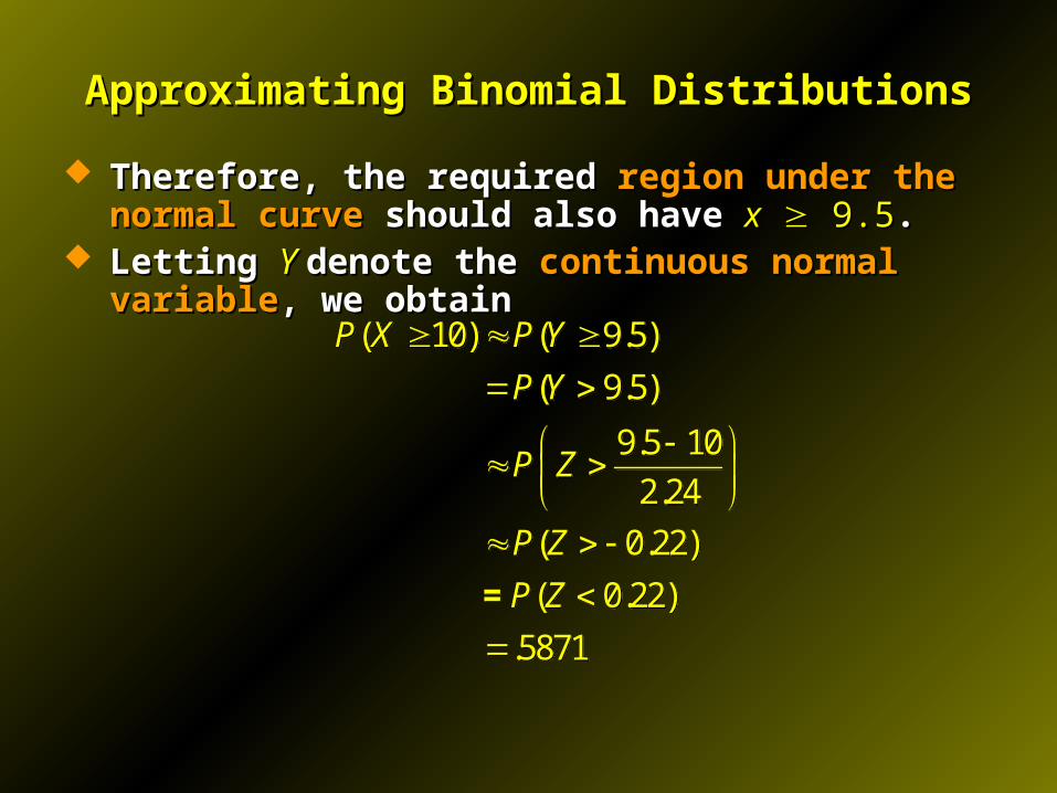
Approximating Binomial DistributionsApproximating Binomial Distributions
Therefore, the required Therefore, the required regionregion under the normal curveunder the normal curve should also have should also have xx 9.5 9.5..
Letting Letting Y Y denote the denote the continuous normal variablecontinuous normal variable, we obtain, we obtain
( 10) ( 9.5)
( 9.5)
9.5 10
2.24
( 0.22)
( 0.22)
.5871
P X P Y
P Y
P Z
P Z
P Z
=
( 10) ( 9.5)
( 9.5)
9.5 10
2.24
( 0.22)
( 0.22)
.5871
P X P Y
P Y
P Z
P Z
P Z
=
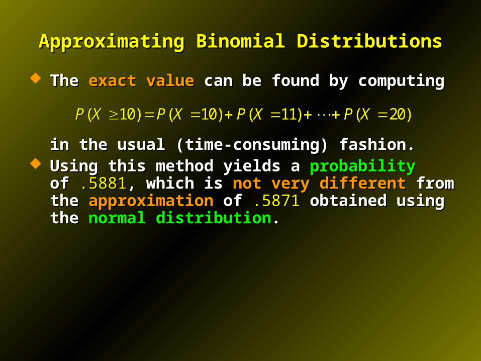
Approximating Binomial DistributionsApproximating Binomial Distributions
The The exact valueexact value can be found by computing can be found by computing
in the usual (time-consuming) fashion.in the usual (time-consuming) fashion. Using this method yields a Using this method yields a probabilityprobability of of .5881.5881, which is , which is not not
very differentvery different from the from the approximationapproximation of of .5871.5871 obtained obtained using the using the normal distributionnormal distribution..
( 10) ( 10) ( 11) ( 20)P X P X P X P X ( 10) ( 10) ( 11) ( 20)P X P X P X P X
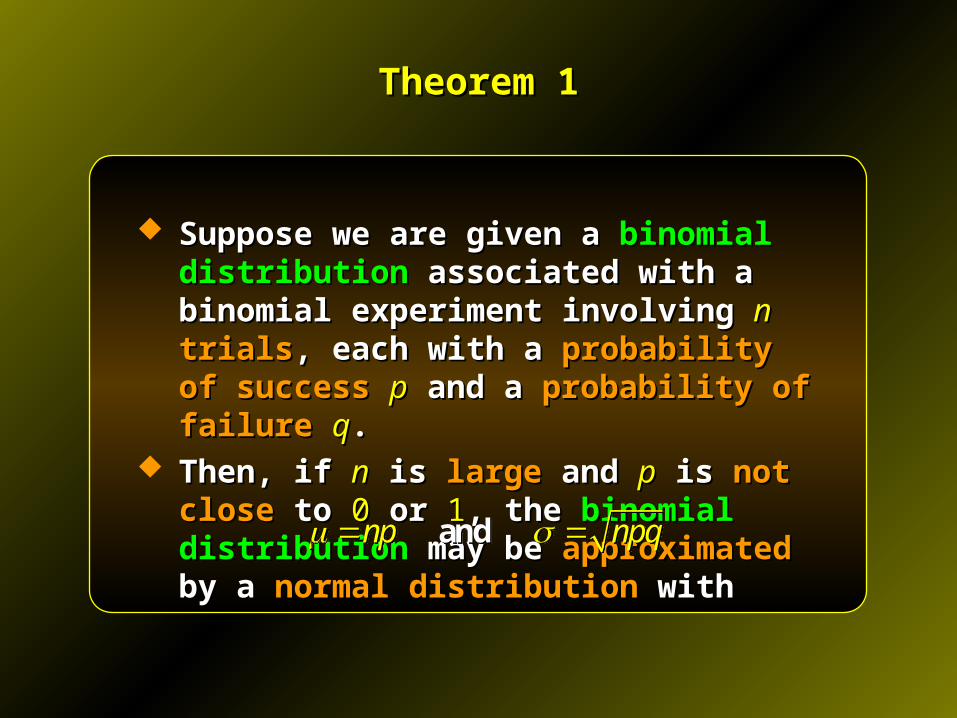
Suppose we are given a Suppose we are given a binomial distributionbinomial distribution associated with a binomial experiment associated with a binomial experiment involving involving nn trialstrials, each with a , each with a probability of probability of successsuccess pp and a and a probability of failureprobability of failure qq..
Then, if Then, if nn is is largelarge and and pp is is not closenot close to to 00 or or 11, , the the binomial distributionbinomial distribution may be may be approximatedapproximated by a by a normal distributionnormal distribution with with
Theorem 1Theorem 1
np npq and np npq and
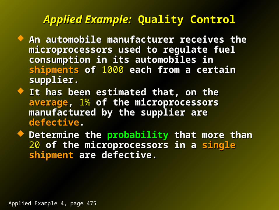
Applied Example:Applied Example: Quality Control Quality Control
An automobile manufacturer receives the An automobile manufacturer receives the microprocessors used to regulate fuel consumption in its microprocessors used to regulate fuel consumption in its automobiles in automobiles in shipmentsshipments of of 10001000 each from a certain each from a certain supplier.supplier.
It has been estimated that, on the It has been estimated that, on the averageaverage, , 1%1% of the of the microprocessors manufactured by the supplier are microprocessors manufactured by the supplier are defectivedefective..
Determine the Determine the probabilityprobability that more than that more than 2020 of the of the microprocessors in a microprocessors in a single shipmentsingle shipment are defective. are defective.
Applied Example 4, page 475
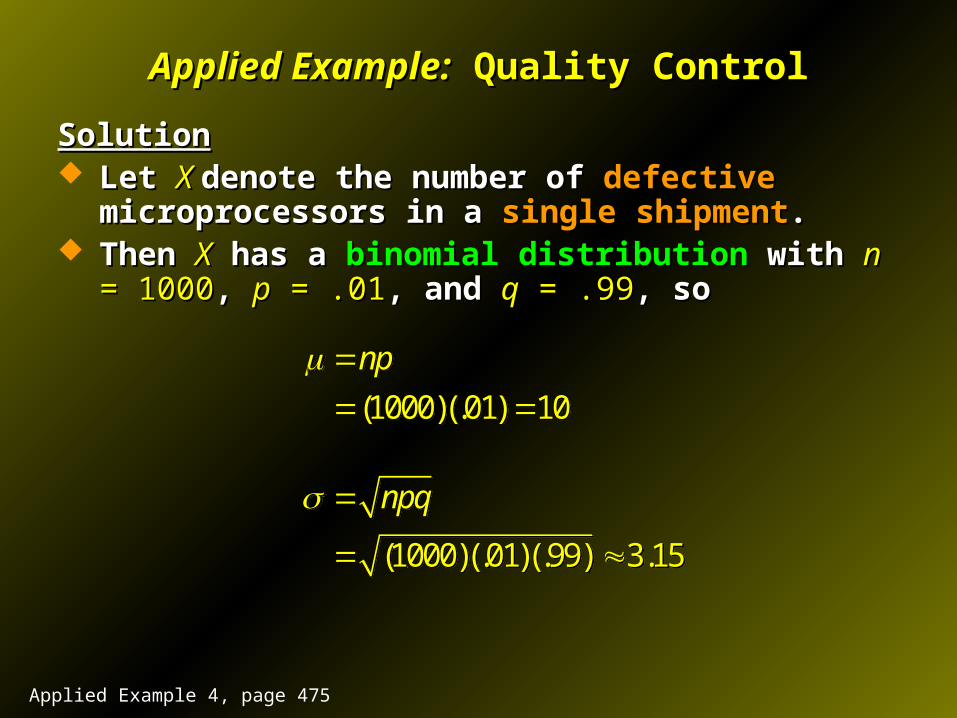
Applied Example:Applied Example: Quality Control Quality Control
SolutionSolution Let Let X X denote the number of denote the number of defectivedefective microprocessors in a microprocessors in a
single shipmentsingle shipment.. Then Then XX has a has a binomial distributionbinomial distribution with with nn = 1000= 1000, , pp = .01= .01, ,
and and qq = .99= .99, so, so
(1000)(.01) 10
(1000)(.01)(.99) 3.15
np
npq
(1000)(.01) 10
(1000)(.01)(.99) 3.15
np
npq
Applied Example 4, page 475
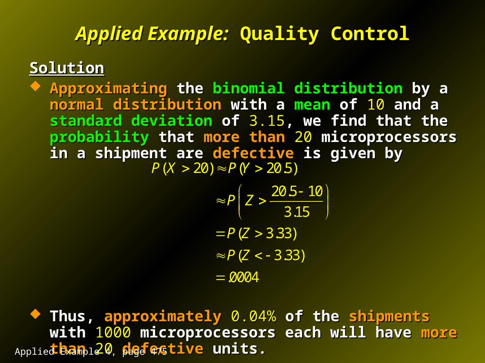
Applied Example:Applied Example: Quality Control Quality Control
SolutionSolution ApproximatingApproximating the the binomial distributionbinomial distribution by a by a normal normal
distributiondistribution with a with a meanmean of of 1010 and a and a standard deviationstandard deviation of of 3.153.15, we find that the , we find that the probabilityprobability that that more thanmore than 2020 microprocessors in a shipment are microprocessors in a shipment are defectivedefective is given by is given by
Thus, Thus, approximatelyapproximately 0.04%0.04% of the of the shipmentsshipments with with 1000 1000 microprocessors each will have microprocessors each will have more thanmore than 2020 defectivedefective units. units.
( 20) ( 20.5)
20.5 10
3.15
( 3.33)
( 3.33)
.0004
P X P Y
P Z
P Z
P Z
( 20) ( 20.5)
20.5 10
3.15
( 3.33)
( 3.33)
.0004
P X P Y
P Z
P Z
P Z
Applied Example 4, page 475

End of End of Chapter Chapter