8.1 Hypothesis Testing Do the data provide sufficient ...stevetoner.com/lec_notes/Toner_notes_8-9_Bluman_8e.pdf · 8.1 Hypothesis Testing A hypothesis is a statement or a claim about

Math 120 – Introduction to Statistics – Mr. Toner’s Lecture Notes

© 2011 Stephen Toner 59

8.1 Hypothesis Testing

A hypothesis is a statement or a claim about

the value of a population parameter. There are

two types of hypotheses:

1. null hypothesis (H0)- assumed to be true

until proven false through the use of sample

data.

2. alternate hypothesis (H1)- what must be

true if Ho is false.

There are 3 types of alternate hypothesis tests:

1. 2-tailed test- when Ho must equal a certain

value, H1 is not equal to it.

2. left-tailed test- when Ho must be at least a

certain value, H1 is less than it.

3. right-tailed test- when Ho can't be more

than a value, H1 says it must be higher.

example: A new car claims to average 35 mpg

for highway driving

H0:

H1: ... two-tailed

To test a claim, assume Ho is true and then

verify whether is within a certain number of

standard deviations of . ( Is within 2

standard deviations to either side of ? )

example: One year, the mean energy

consumed per U.S. household was 103.6

million British thermal units (BTU). For that

same year, 20 randomly selected households in

the West had the following energy

consumptions, in millions of BTU.

104 80 82 70 84 78 61 65 72 74

94 83 95 76 65 76 69 81 100 84

Do the data provide sufficient evidence to

conclude that the mean energy consumption by

western households differed from that of all

U.S. households? Assume that the standard

deviation of energy consumptions of all

western households was 15 million BTU.

a) State the null and alternate hypotheses.

b) Obtain a precise criterion for deciding

whether or not to reject the null hypothesis

in favor of the alternate hypothesis.

c) Apply your criterion in part (b) to the

sample data and state your conclusion.


60 © 2011 Stephen Toner

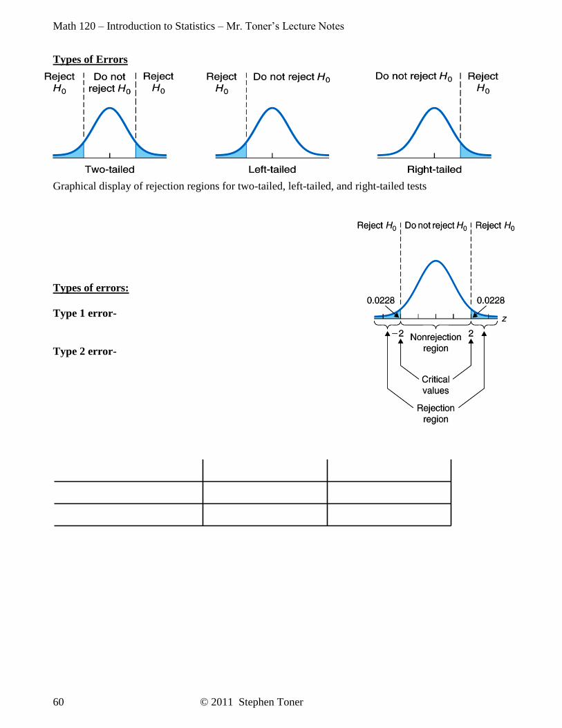
Types of Errors

Graphical display of rejection regions for two-tailed, left-tailed, and right-tailed tests

Types of errors:

Type 1 error-

Type 2 error-



Probability of Type 1 and Type 2 errors:

• The significance level of a hypothesis

test is the probability of making a Type 1

error, rejecting a true null hypothesis.

• (beta) denotes the probability of making

a Type 2 error.

• For a fixed sample size, the smaller the

Type 1 error probability, the larger the

Type 2 error probability (and vice versa).

There are 2 possible conclusions of a

hypothesis test:

If Ho is rejected, conclude that H1 is

probably true (the data seems to suggest

that…); or,

If Ho is accepted, conclude that the data

"do not provide sufficient evidence to

conclude that < the alternate hypothesis. >"

example: Ten years ago, the mean age of

juveniles held in public custody was 16.0 years.

The ages of a random sample of juveniles

currently being held in public custody are to be

used to decide whether this year's mean age of

all juveniles held in public custody is less than

it was 10 years ago. The null and alternate

hypotheses for the hypothesis test are:

Ho: = 16.0 years

H1: < 16.0 years,

where is this year's mean age of all juveniles

being held in public custody. Explain what

each of the following would mean.

a) a Type 1 error-

b) a Type 2 error-

c) a correct decision-

Now suppose the results of carrying out the

hypothesis test lead to rejection of the null

hypothesis, = 16.0 years, that is, to the

conclusion < 16.0 years. Classify that

conclusion by error type or as a correct

decision if in fact this year's mean age, , of

all juveniles being held in public custody

d) is 16.0 years.

e) is less than 16.0 years.

8.2 Z-Tests for a Mean

Suppose a hypothesis test is to be performed at

significance level . Then the critical values

must be chosen so that if Ho is true, the

probability is equal to that the test statistic is

in the rejection region. A Z-test is typically

used when the sample size is large (n 30)

or normally distributed and is known.

General Procedure for Z-test (Classical

Approach):

Assumptions: a. Normal population or large samples

b. known

1. State Ho and H1.

2. Determine significance level . (This will

always be given to you.)

Find the critical values:

a) 2-tailed... use InvNorm( /2)

b) left-tailed... use InvNorm( )

c) right-tailed...use -InvNorm( )

The value of the test statistic is found when

you perform a Z-test on your TI-83.

Decide whether to accept or reject Ho. Is

the test statistic in the acceptance or

rejection region?

6. State your conclusion in words. (use

statistical doublespeak)



example: A car manufacturer states that its

new model averages 35 mpg. Assume the

population's mpg is normally distributed with

=10 mpg. A sample of size n=64 cars is

taken which yields x =30. Test the

manufacturer's hypothesis at =0.05

significance.

step 1: Ho:

H1:

step 2: =

step 3: critical value(s):

step 4: test statistic:

step 5: decision:

step 6: conclusion:

example: The mean daily room charge for a

semi-private room in US hospitals in 1998 was

$253. In that same year, a random sample of

30 Massachusetts hospitals yielded a mean

daily semi-private room charge of $260.68 with

a standard deviation of $12.77. At the 5%

significance level, do the data provide

sufficient evidence to conclude that in 1998 the

mean daily semi-private room charge in

Massachusetts hospitals exceeded the national

mean of $253?

step 1: Ho:

H1:

step 2: =

step 3: Which Test?

step 4: test statistic and P-value:

step 5: decision:

step 6: conclusion:



The P-value of a hypothesis test is the

observed significance level of a hypothesis test.

It is the probability (within the rejection region)

to the right or left of the test statistic, rather

than to the right of the critical value.

Therefore, the smaller the P-value, the

stronger the evidence against the null

hypothesis.

Quite often when we reject a null hypothesis,

we find that the test statistic is far into the

rejection region. The P-value helps denote this,

telling the reader of the hypothesis test just

how strong the rejection actually was.

There are many critics of the 95% hypothesis

test. The use of the P-value for a test rather

than doing a accept/reject conclusion is gaining

popularity in current literature.

Guidelines for using the P-value to assess the evidence against the null hypothesis:

Comparison of critical-value and P-value approaches:



example: Ten years ago, the mean age of

juveniles held in public custody was 16.0 years.

The mean age of 250 randomly selected

juveniles currently being held in public custody

is 15.86 years. Assuming =1.01 years, does

it appear that the mean age, , of all juveniles

being held in public custody this year is less

than it was 10 years ago? Perform the

appropriate hypothesis test using =0.10.

8.3 T-test for a Mean

A T-test is performed when is unknown

and the population under is known to be

normally distributed (or is large enough so

that the sampling mean will be approximately

normally distributed.)

General Procedure for T-test (Classical

Approach):

Assumptions: a. Normal population or large samples

b. unknown

1. State Ho and H1.



3. Find the critical values: (use the t-table with

df=n-1 or the program INVERSE )

a) 2-tailed... use 2t

b) left-tailed... use t

c) right-tailed... use t

The value of the test statistic is found when

you perform a t-test on your TI-83, using

ns

xt

as the test statistic.

Decide whether to accept or reject Ho. Is

the test statistic in the acceptance or

rejection region?

6. State your conclusion in words.

Note the components of a confidence interval:

alpha, the significance level

the standard deviation

the sample size



example: In 1987, the mean verbal SAT score

was 430 out of 800. Last year a sample of 25

randomly selected scores was taken, yielding

the following scores:

346 491 381 420 494 496 360 303 485

289 352 385 434 446 436 378 500 562

479 516 315 558 496 422 615

At the 10% significance level, have SAT scores

improved over the 1987 mean of 430 points?

step 1: Ho:

H1:

step 2: =

step 3: Which Test?

step 4: test statistic and P-value:

step 5: decision:

step 6: conclusion:

Referring to the example above, find and

interpret a 90% confidence interval for the

mean verbal SAT score last year.

example: A paint manufacturer claims that the

average drying time for its new latex paint is 2

hours. To test that claim, the drying times are

obtained for 20 randomly selected cans of

paint. Here are the drying times, in minutes.

123 109 115 121 130

127 106 120 116 136

131 128 139 110 133

122 133 119 135 109


conclude that the mean drying time is greater

than the manufacturer’s claim of 120 minutes?

Use 05.0 .

step 1: Ho:

H1:

step 2: =

step 3: Which Test?

step 4: test statistic:

step 5: decision:

step 6: conclusion:

Referring to the example above, find a 90%

confidence interval for the mean drying time of

this new latex paint.



8.4 Z-Test for a Proportion

Assumptions: np and n(1-p) both 5,

simple random samples

General Procedure:

1. State Ho and H1.



Find the value of the test statistic and the P-

value using your calculator.

4. Decide whether to accept or reject Ho based

upon P.

5. State your conclusion in words.

example: A college is considering construction

of a new parking lot because it feels at least

60% of all students drove to campus. If a

random sample of n=250 students contains 165

drivers, can the administration's claim be

rejected at a 3% level of significance?

Confidence interval:

example: A survey of 379 people who viewed

the Reagan/Mondale debate resulted in 205

who thought that Mondale won the debate.

With 5% significance, can we infer that the

majority of all registered voters who watched

the debate also thought that Mondale did

better?

Confidence interval:



9.1 Comparing Population Means

Sometimes we wish to compare 2 different populations to make a decision.

example: Let's say that Mr. Toner teaches two

sections of the same class and wishes to

compare their mean class scores.

We could use the following hypotheses:

After calculating each sample mean, a criterion

needs to be established to determine how great

a difference between means is acceptable. To

determine the criterion, you must look at the

sampling difference between the two means.

There are 3 types of alternate hypotheses

when Ho:

a) 2-tailed...

b) left-tailed...

c) right-tailed...

example: The U.S. National Center for Health

Statistics compiles data on the length of stay by

patients in short-term hospitals and publishes

its findings in Vital and Health Statistics.

Independent samples of 39 male patients and

35 female patients gave the following data on

length of stay, in days.

a. Do the data provide sufficient evidence to

conclude that, on the average, the lengths of

stay in short-term hospitals by males and

females differ? Assume 4.51 days and

6.42 days. Perform the appropriate

hypothesis test at the 5% significance level.

b. Determine a 95% confidence interval for

the differences between the mean

lengths of stay in short-term hospitals by

males and females.

Male Female

4 4 12 18 9 14 7 15 1 12

6 12 10 3 6 1 3 7 21 4

15 7 3 13 1 1 5 4 4 3

2 10 13 5 7 5 18 12 5 1

1 23 9 2 1 7 7 2 15 4

17 2 24 11 14 9 10 7 3 6

6 2 1 8 1 5 9 6 2 14

3 19 3 1



9.2 Comparing Population Means (2-

Sample t test)

Suppose 1n and 2n are from normally

distributed populations. Also suppose that the

samples are taken independently. If the

population standard deviations can be assumed

to be equal, then we “pool” the sample standard

deviations together.

Assumptions:

1. independent samples

2. normal populations (or large samples)

3. equal population standard deviations (but

unknown sometimes)

When considering the pooled t-test, it is

important to watch for outliers. The presence

of outliers calls into question the normality

assumption. And even for large samples,

outliers can sometimes unduly affect a pooled

t-test because the sample mean and sample

standard deviation are not resistant to them.

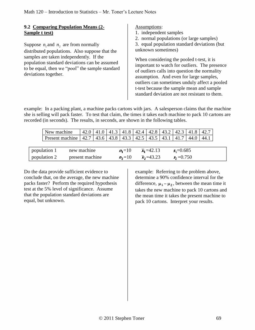
example: In a packing plant, a machine packs cartons with jars. A salesperson claims that the machine

she is selling will pack faster. To test that claim, the times it takes each machine to pack 10 cartons are

recorded (in seconds). The results, in seconds, are shown in the following tables.

New machine 42.0 41.0 41.3 41.8 42.4 42.8 43.2 42.3 41.8 42.7

Present machine 42.7 43.6 43.8 43.3 42.5 43.5 43.1 41.7 44.0 44.1

population 1 new machine =10 =42.13 =0.685

population 2 present machine =10 =43.23 =0.750


conclude that, on the average, the new machine

packs faster? Perform the required hypothesis

test at the 5% level of significance. Assume

that the population standard deviations are

equal, but unknown.

example: Referring to the problem above,

determine a 90% confidence interval for the

difference, , between the mean time it

takes the new machine to pack 10 cartons and

the mean time it takes the present machine to

pack 10 cartons. Interpret your results.



example: Researchers studying obesity

wanted to compare the effectiveness of dieting

with exercise to dieting without exercise. 73

patients were randomly divided into two

groups. Group 1, composed of 37 patients, was

put on a program of dieting with exercise.

Group 2, composed of 36 patients, dieted only.

The results for weight loss, in pounds, after 2

months are summarized as follows: (Assume

that both sets of data are normally distributed.)

GROUP 1 =37 =16.8 lb =3.5 lb

GROUP 2 =36 =17.1 lb =5.2 lb

a) At the 0.05 significance level, determine

whether there is a difference between the two

treatments.

b) Identify the study as a designed experiment

or an observational study. Explain your

answer.

The pooled problems only works when .

If you aren't sure, or if it has not been stated,

you must use the non-pooled-t test.

Assumptions:

independent samples

normal populations

Example: The following are ACT results for

college-bound students, broken down by

gender.

population 1 male =15 =18.3 =3.8

population 2 female =15 =16.2 =4.0

If you cannot assume that the population

standard deviation of test scores for males

and females are equal, does it appear that

college-bound males are, on the average,

outperforming college-bound females in the

math portion of the ACT? Test at a 5%

significance level.

Same question, but use a 10% significance

level.

c) Are the results the same? Why or why not?



9.3 Paired Samples (not independent)

Sometimes you wish to examine the mean

value of a population before and after some

stimulus cause a change. Since the samples are

chosen from the same population, they aren't

necessarily independent.

example: 10 balding men are in an experiment.

Their mean hair density is measured both

before and after a hair tonic is applied in order

to determine whether the hair tonic increased

the mean hair density. This is a paired sample

experiment. We wish to determine if the

difference is significant.

You will need to “trick” your calculator so that

you can pair the data.

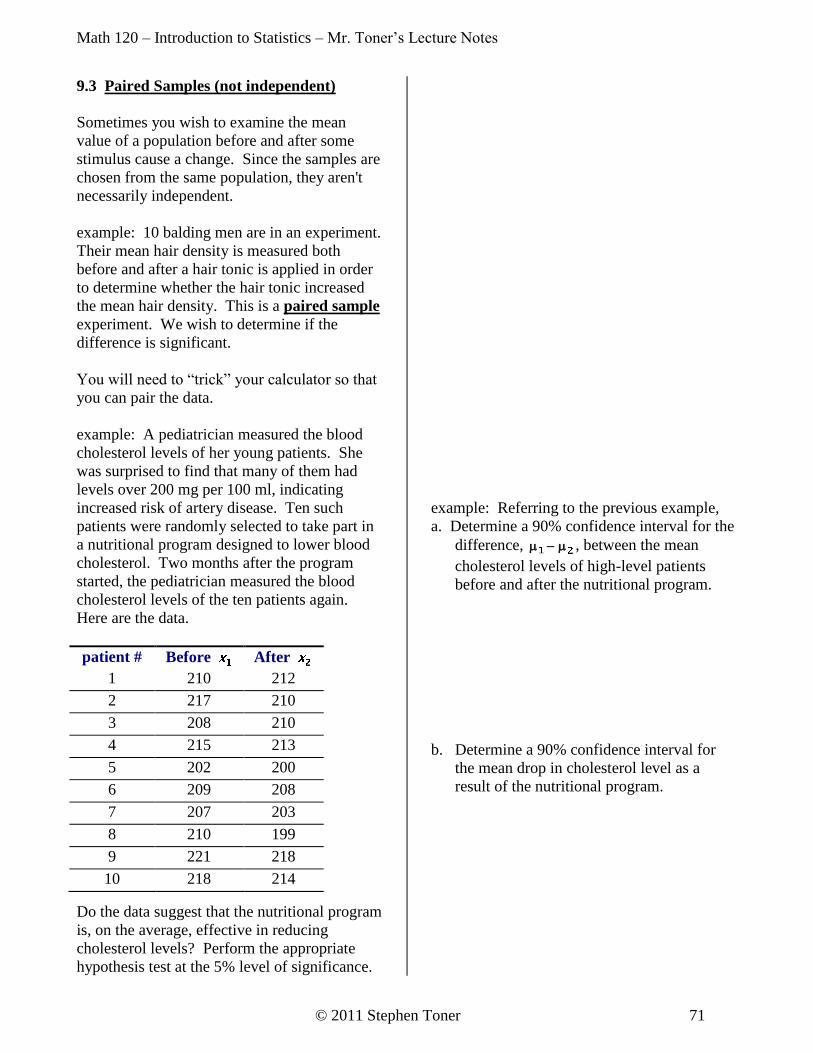
example: A pediatrician measured the blood

cholesterol levels of her young patients. She

was surprised to find that many of them had

levels over 200 mg per 100 ml, indicating

increased risk of artery disease. Ten such

patients were randomly selected to take part in

a nutritional program designed to lower blood

cholesterol. Two months after the program

started, the pediatrician measured the blood

cholesterol levels of the ten patients again.

Here are the data.

Do the data suggest that the nutritional program

is, on the average, effective in reducing

cholesterol levels? Perform the appropriate

hypothesis test at the 5% level of significance.

example: Referring to the previous example,

a. Determine a 90% confidence interval for the

difference, , between the mean

cholesterol levels of high-level patients

before and after the nutritional program.

b. Determine a 90% confidence interval for

the mean drop in cholesterol level as a

result of the nutritional program.

patient # Before After

1 210 212

2 217 210

3 208 210

4 215 213

5 202 200

6 209 208

7 207 203

8 210 199

9 221 218

10 218 214



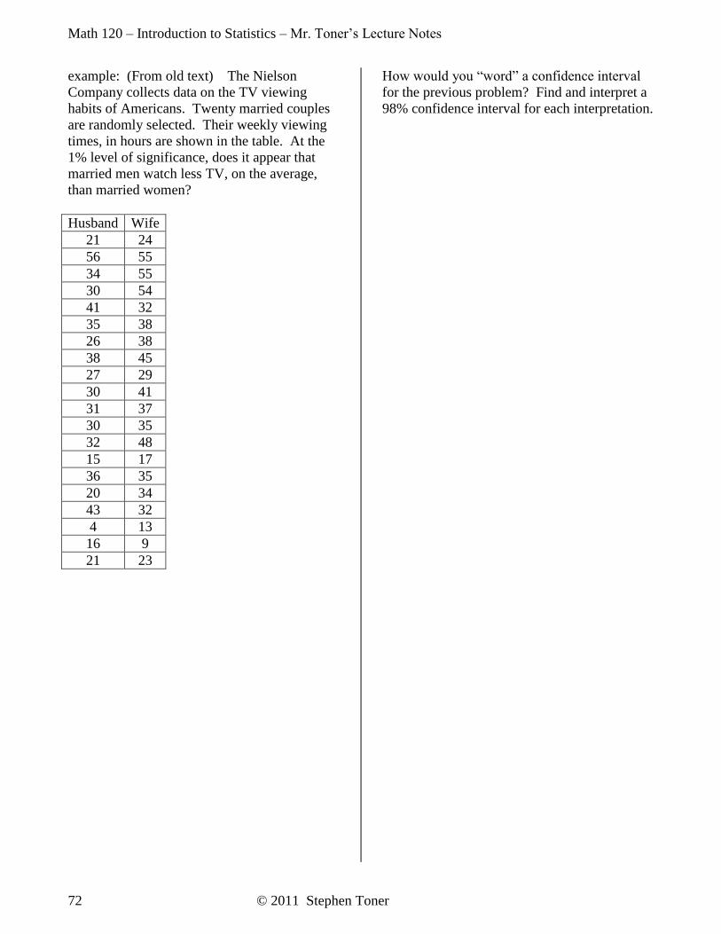
example: (From old text) The Nielson

Company collects data on the TV viewing

habits of Americans. Twenty married couples

are randomly selected. Their weekly viewing

times, in hours are shown in the table. At the

1% level of significance, does it appear that

married men watch less TV, on the average,

than married women?

Husband Wife

21 24

56 55

34 55

30 54

41 32

35 38

26 38

38 45

27 29

30 41

31 37

30 35

32 48

15 17

36 35

20 34

43 32

4 13

16 9

21 23

How would you “word” a confidence interval

for the previous problem? Find and interpret a

98% confidence interval for each interpretation.



9.4 Comparing Population Proportions of

Different Populations

Assumptions:

1. independent samples

2. n1p1, n1(1-p1), n2p2, n2(1-p2) are all at least 5

Here we are pooling the proportions when we

calculate pp̂ because the standard deviations of

each population may differ. The margin of

error, E, is half the confidence interval;

likewise the sample size can be found (having

an error of at most E) using the formula

example: In April and May 1985, the Gallup

organization conducted a poll to estimate the

percentage of Americans who approved of how

President Reagan was handling his job. At the

5% significance level, do the data suggest that

the percentage of those who approved of

Reagan increased from April to May 1985?

population 1 April = 0.5203

population 2 May = 0.5497

Construct a 90% confidence interval for the

differing percentages of those Americans who

approve of Reagan from April to May 1985

( ).

Example: The Organization for Economic

Cooperation and Development summarizes

data on labor-force participation rates.

Independent samples were taken of 300 U.S.

women and 250 Canadian women. Of the U.S.

women, 211 were found to be in the labor

force; of the Canadian women, 170 were found

to be in the labor force. At the 5% significance

level, do the data suggest that there is a

difference between the labor-force participation

rates of U.S. and Canadian women?

Find and interpret a 95% confidence interval

for the difference , between the labor

force participation rates of U.S. and Canadian

women.



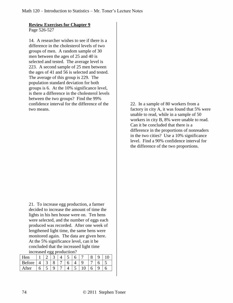
Review Exercises for Chapter 9 Page 526-527

14. A researcher wishes to see if there is a

difference in the cholesterol levels of two

groups of men. A random sample of 30

men between the ages of 25 and 40 is

selected and tested. The average level is

223. A second sample of 25 men between

the ages of 41 and 56 is selected and tested.

The average of this group is 229. The

population standard deviation for both

groups is 6. At the 10% significance level,

is there a difference in the cholesterol levels

between the two groups? Find the 99%

confidence interval for the difference of the

two means.

21. To increase egg production, a farmer

decided to increase the amount of time the

lights in his hen house were on. Ten hens

were selected, and the number of eggs each

produced was recorded. After one week of

lengthened light time, the same hens were

monitored again. The data are given here.

At the 5% significance level, can it be

concluded that the increased light time

increased egg production?

Hen 1 2 3 4 5 6 7 8 9 10

Before 4 3 8 7 6 4 9 7 6 5

After 6 5 9 7 4 5 10 6 9 6

22. In a sample of 80 workers from a

factory in city A, it was found that 5% were

unable to read, while in a sample of 50

workers in city B, 8% were unable to read.

Can it be concluded that there is a

difference in the proportions of nonreaders

in the two cities? Use a 10% significance

level. Find a 90% confidence interval for

the difference of the two proportions.

Documents

8.1 Hypothesis Testing Do the data provide sufficient ...stevetoner.com/lec_notes/Toner_notes_8-9_Bluman_8e.pdf · 8.1 Hypothesis Testing A hypothesis is a statement or a claim about