8.1 representation of periodic sequences:the discrete fourier series8.2 the fourier transform of periodic signals8.3 properties of the discrete fourier series8.4 fourier representation of finite-duration sequences:

Definition of the discrete fourier transform8.5 sampling the fourier transform(point of sampling)8.6 properties of the fourier transform8.7 linear convolution using the discrete fourier transform8.8 the discrete cosine transform(DCT)

Chapter 8 the discrete fourier transform

8.1 representation of periodic sequences:the discrete fourier series

NknjknN

N

n

knN

N

k

knN

eW

NkWnxkX

NnWkXN

nx

/2

1

0

~~

1

0

~~

1,..0),2(][][

1,..0),1(][1

][

][~)(

][~][~ 1

0

kXN

nrNkWnxrNkX

N

n

)10/sin(

)2/sin(][

4

0

10/410

~

k

keWkX

n

kjkn

Figure 8.1

EXAMPLE.

N=10

Figure 8.2

phase X denotes ： magnitude=0 ， phase is indeterminate

8.2 the fourier transform of periodic signals

1

0 0

22][

~)

2(][

~2)(

~ N

k

j

other

kNN

kXN

kkX

NeX

dispersion in time domain results in periodicity in frequency domain;

Periodicity in time domain results in dispersion in frequency domain.

DFS is a method to calculate frequency spectrum of periodic signals.

FIGURE 8.5

][~

][~],[~

][~],[~

][~2211 kX

DFSnxkX

DFSnxkX

DFSnx

8.3 properties of the discrete fourier series

][~

][~

][~][~:.1 2121 kXbkXaDFS

nxbnxalinearity

N=4 ， 12 points DFS

N=6 ， 12 points DFS

compositive sequence N=12 ， 12 points DFS

two periodic sequences with different period

both period=12

][~

][~:.2 kXN

kmW

DFSmnxsequenceaofshift

][~

][~ lkXDFS

nxN

nlW

][~][~

:.3 kxNDFS

nXduality

[k]*X~DFS

n][*x~k],[*X~DFS

[n]*x~

:properties4.symmetry

[k]X~

k])[*X~

[k]X~

(2

1DFS[n])*x~[n]x~(

2

1[n]}x~Re{ e

[k]X~

k])[*X~

[k]X~

(2

1DFS[n])*x~[n]x~(

2

1[n]}x~jIm{ o

]}[X~

Re{[k])*X~

[k]X~

(2

1DFSn])[*x~[n]x~(

2

1[n]x~e k

]}[~

Im{])[*~

][~

(2

1])[*~][~(

2

1][~ kXjkXkX

DFSnxnxnxo

][*][~~

nxnx

][~

][~

|][~

||][~

|

]}[~

Im{]}[~

Im{

]}[~

Re{]}[~

Re{

kXkX

kXkX

kXkX

kXkX

][*~

][~

kXkX

For a real sequence:

FIGURE 8.2

EXAMPLE. DFS of real sequence

][~][~][~][~][~][~][~

:.5

12

1

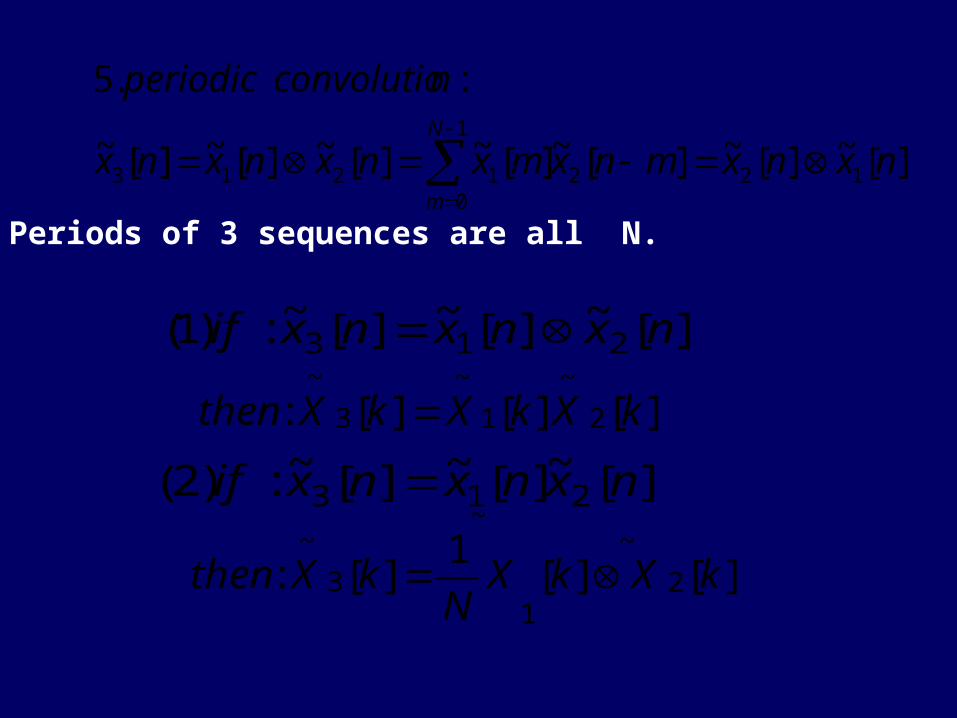
021213 nxnxmnxmxnxnxnx

nconvolutioperiodicN

m

][~][~][~:)1( 213 nxnxnxif

][][][: 2

~

1

~

3

~kXkXkXthen

][~][~][~:)2( 213 nxnxnxif

][][1

][: 2

~

1

~

3

~kXkX

NkXthen

Periods of 3 sequences are all N.

Figure 8.3

graphic method to calculate periodic

convolution

8.4 fourier representation of finite-duration sequences:

Definition of the discrete fourier transform ]))[((]mod[][][~

Nr

nxNnxrNnxnx

][][~][ nRnxnx N

Figure 8.8

EXAMPLE.

The last two expressions are only suitable to no aliasing.

Two derivations of definition:

1. Periodic extension of the finite-duration sequence with period N ;

DFS of the periodic sequence ;

DFT is the dominant period of DFS.

2. DTFT of the finite-duration sequence;

DFT is the N-points spectral sampling.

kNjezk

N

j zXeXkX

2|)(|)(][ 2

NnWkXN

nx

NkWnxkX

N

k

knN

N

n

knN

,...1,0,][1

][

1,....1,0,][][

1

0

1

0

duration of sequence is N

1

0

1

0

][1

]0[

][]0[

N

k

N

n

kXN

x

nxX

Figure 8.10

EXAMPLE.

]}[~{ nxDFS

][][ 5

~

kRkX

]))[(( 5nx

periodic extension

with period 5

explanations ： 1. DFT and DFS have the same expression, but DFT are samples of frequency spectrum of the finite-duration sequence , DFS is frequency spectrum of periodic sequence 。 2. the periods of DFS in time and frequency domain is N, DFT in frequency domain is defined to be finite duration, but has the immanent period N 。 3. the meaning of DFT not only is samples of frequency spectrum , but also can reconstruct time-domain signal 。

8.5 sampling the fourier transformEXAMPLE.

Figure 8.5

periodic extension with

period 10

reflect frequency spectrum of signal more truly than figure 8.10

conclusion ： sequence with length N is extended to M by filling 0 in time domain, then do M-points DFT. We can get more dense samples of its FT, and can reconstruct time-domain signal by taking the first N nonzero values from the reconstructed signal 。 contrarily, if we want to get M-points samples of FT by DFT, we can use the method of filling 0 in time domain.

1...1,0,][|)( 2

MkWnxeXn

knM

kM

j

][)][(][' nRrMnxnx Nr

genetic instance ：

Sequence with length N （ or infinite length ） , sample M points in frequency domain （ more than or less than or equal to N ），then the reconstructed time-domain signal is dominant period of the periodic extension with period M of original signal （ maybe aliasing ）。 Viz. if

then the result of IDFT is ：

Conclusion ： when M<N, the reconstructed time-domain signal is domain period of the periodic extension with aliasing of original signal. Contrarily , if we want to get M (M<N) sample points of FT by DFT ， we can extend the sequence with period M in time domain, take the dominant period and do M-points DFT.

sampling theorem in frequency domain ：If sampling points N in frequency domain is more than the length of sequence ， the time-domain signal can be reconstructed ；and the sampling spectral line can be constructed to be continuous spectral function by ideal interpolation ：

1

0 1

][/1)(

N

kjk

N

Njj

eW

kXNeeX

1

0

1

0

1

0

1

0

1

0

1

0

1

][/1

)]([1

)][1

(][)(

:

N

kjk

N

Nj

njN

k

N

n

knN

njN

n

N

k

knN

N

n

njj

eW

kXNe

eWkXN

eWkXN

enxeX

prove

)(][ 11jFT

eXnx

][][][][ 2

points

2 nRrMnxnxkX Mr

IDFTM

r

IDFSMrMnxnxkX ][][~][

~33

点

M点取样

M点取样

DFT of a finite-duration sequence 、 DFS of a periodic sequence are both samples of FT of another sequence, then the relationship among the three sequences in time domain ：

periodic extension in time domainsampling in frequency domain

取长为M的主周期

summary 8.5

1. DFT is N-points samples of frequency spectrum of sequence with length N. the more spectral sampling points, the more genuine to reflect the frequency spectrum

2. get M-points spectral samples of N-points sequence by M-points DFT:

（ 1 ） M=N ， do M-points DFT directly

（ 2 ） M>N ， extend x[n] to M points by filling 0 ， then do M-points DFT

（ 3 ） M<N ， periodic extension of x[n] with period M and aliasing ， take the dominant period with length M, then do M-points DFT

3. whether spectral sampling can reconstruct original time-domain signal

spectral sampling theorem ： if spectral sampling points is larger than or equal to the length of signal, the time-domain signal can be reconstructed. Contrarily, it can not be done.

4. If frequency spectrum is the same ， its samples are equal ； contrarily, it does not come into existence 。 if frequency spectrum has linear phase, its samples has linear phase, too ； co

ntrarily, it does not come into existence 。

][][],[][],[][ 2211 kXDFT

nxkXDFT

nxkXDFT

nx

8.6 properties of the fourier transform

][][][][:.1 2121 kbXkaXDFT

nbxnaxlinearity

2.circular shift of a sequence

][])))([((][]))[((][1 nRmNnxnRmnxnx NNNN

][][]))[(( kXN

kmW

DFTnRmnx NN

][]))[((][ln

kRlkXDFT

nxN

W NN

Figure 8.12

EXAMPLE.

circular shift

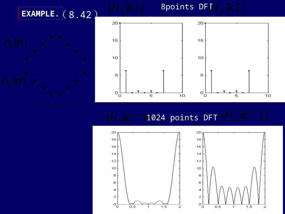
（ 8.42）EXAMPLE.

][1 nh

][2 nh

8points DFT|][| 1 kH |][| 2 kH

1024 points DFT|)(| 1jeH |)(| 2

jeH

][][]))[((][:.3 kNNxkRkNxDFT

nXduality NN

)2.0cos(][ nnnx

|]}[{||][| nxDFTkX

]}[{ nXDFT

EXAMPLE.

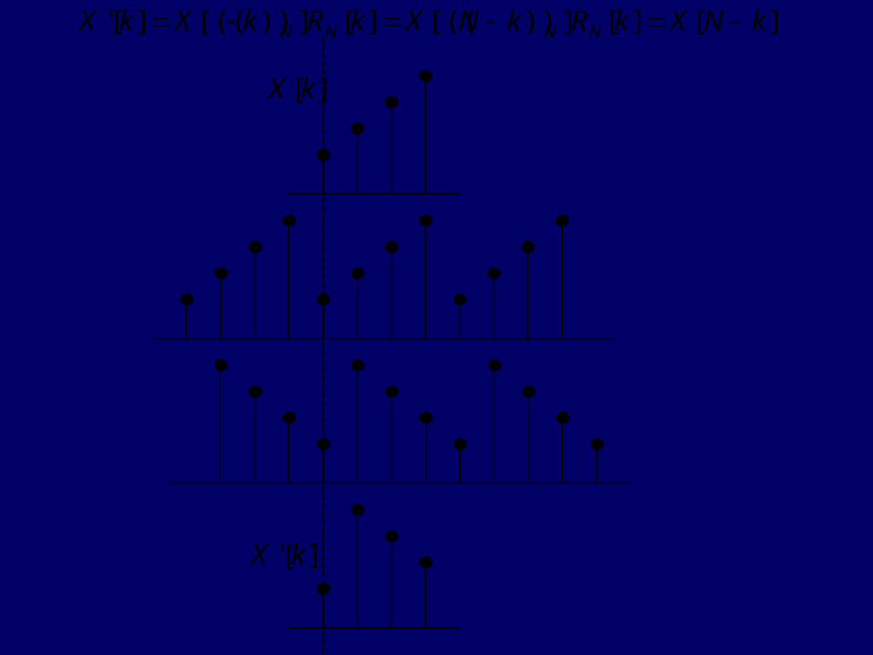
][][]))[((][]))[((][' kNXkRkNXkRkXkX NNNN

][kX

][' kX

][][]))[((][]))[((][ **** kNXkRkNXkRkXDFT

nx NNNN

][][][]))[(( *** kXDFT

nNxnRnx NN

4. Symmetry properties:

]}[Re{])[*][(2

1])[*][(

2

1][ kXkXkX

DFTnNxnxnxep

][])[*][(2

1])[*][(

2

1]}[Re{ kXkNXkX

DFTnxnxnx ep

][])[*][(2

1])[*~][~(

2

1]}[~Im{ kXkNXkX

DFTnxnxnxj op

]}[Im{])[*][(2

1])[*][(

2

1][ kXjkXkX

DFTnNxnxnxop

symmetriceven ispart imaginary , symmetric odd ispart real

lenth ][*])[*][(2

1][

symmetric odd ispart imaginary , symmetriceven ispart real

length ][*])[*][(2

1][

while

][][][

decomposed becan length with sequence

components ricantisymmet-conjugate periodic:][

components symmetric-conjugate periodic:][

definition

NkNXkNXkXkX

NkNXkNXkXkX

kXkXkX

N

kX

kX

opop

epep

opep

op

ep

，

，

：

：

：

][*][ kNXkX

For a real sequence:

][][

|][||][|

kNXkX

kNXkX

]}[Im{]}[Im{

]}[Re{]}[Re{

kNXkX

kNXkX

][*][ nxnx

N=10EXAMPLE.

DFT of real sequence9...0),5.0cos(5.0][ nnnx n

Real{X[k]} Imag{X[k]}

|X[k]| arg{X[k]}

N=9

|X[k]|

Arg{X[k]}

5.circular convolution

][])))[((]))[((( 21 nRnxnx NNN

][][][)]([)1( 2121 kXkXDFT

nxNnx

][)]([1

][][)2( 2121 kXNkXN

DFTnxnx

][)]([][ 21 nxNnxny

1

0

21 ][])))[((]))[(((N

m

NNN nRmnxmx

Length of x1[n],x2[n],y[n] are N.

][]))1[((

]1[)]([

nRnx

nNnx

NN

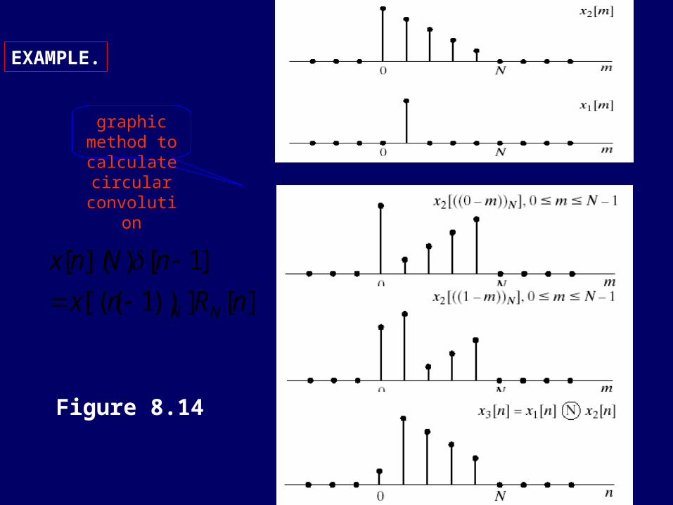
Figure 8.14

EXAMPLE.

graphic method to calculate circular

convolution

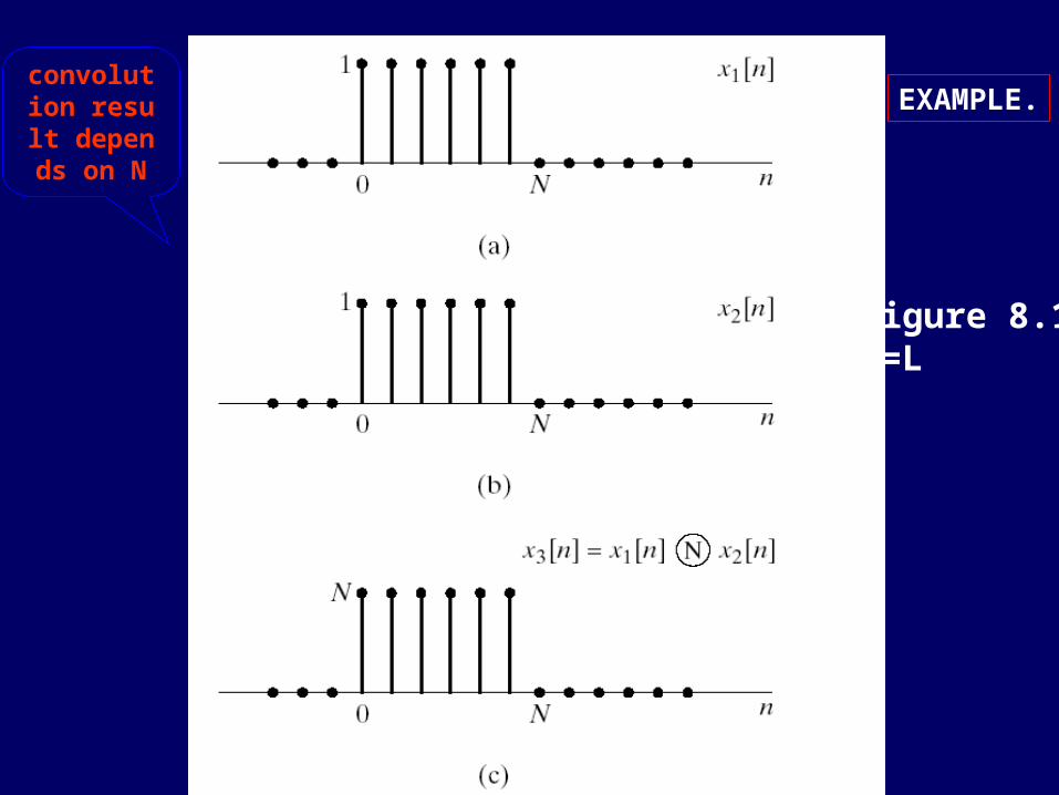
Figure 8.15N=L

EXAMPLE.convolution result depen

ds on N

Figure 8.16 N=2L

EXAMPLE.

1

0

1

0

][*][1

][*][N

k

N

n

kYkXN

nynx

6.paswal’s theory

1

0

21

0

2 |][|1

|][|N

k

N

n

kXN

nx

8.7 linear convolution using the discrete fourier transform

][][][][:

][*][][:

nRrNnynhNnxthen

nhnxnyif

N

r

）（

][][][ nynhnx

][)]([ nhNnx

)()( jj eHeX

][][ kHkXN point sample

IDFT

][][ nRrNny N

r

][kY

)( jeY

according to properties of circular

convolution

according to spectral

sampling

FT

PROVE

If N>=N1+N2-1,then x[n]*h[n]=x[n](N)h[n]

Figure 8.18

EXAMPLE.

linear convolution

shift right of the linear convolution

shift right of the

linear convolution

6 points circular convolution= linear convolution with aliasing

12 points circular convolution= linear convolution

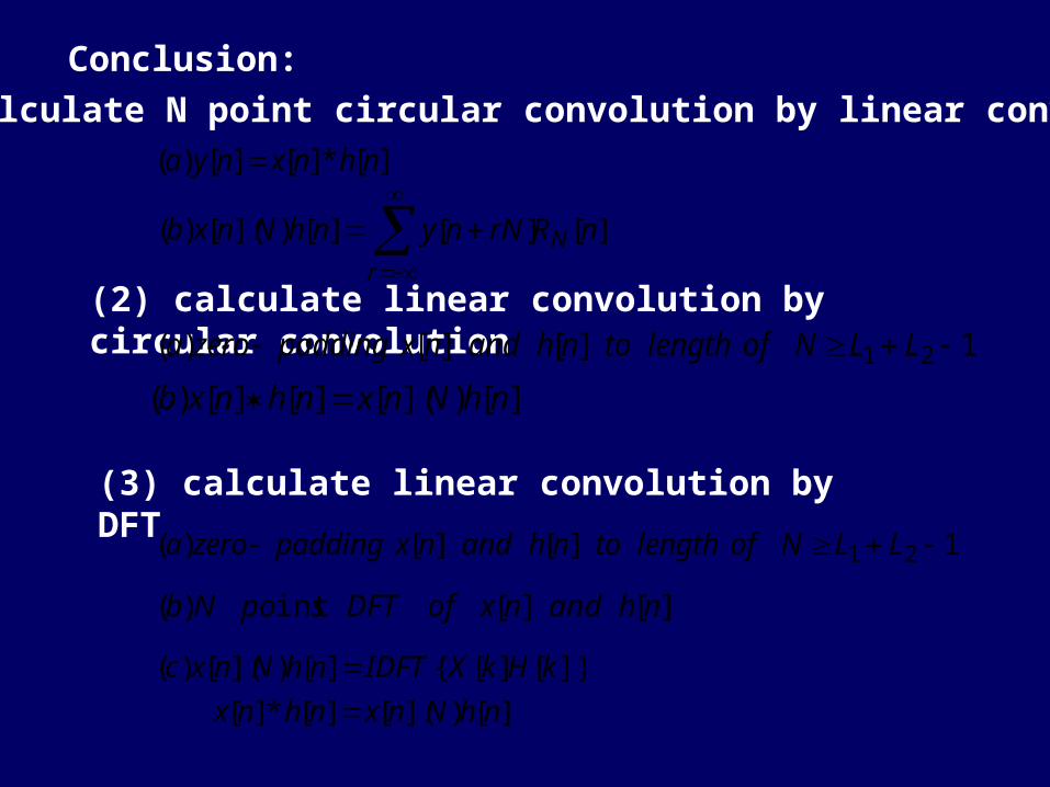
Conclusion:

][*][][)( nhnxnya

(2) calculate linear convolution by circular convolution

1][][)( 21 LLNoflengthtonhandnxpaddingzeroa

1][][)( 21 LLNoflengthtonhandnxpaddingzeroa

(1)calculate N point circular convolution by linear convolution

(3) calculate linear convolution by DFT

][][][)]([)( nRrNnynhNnxb N

r

][)]([][][)( nhNnxnhnxb

][][int)( nhandnxofDFTspoNb

][)]([][*][

]}[][{][)]([)(

nhNnxnhnx

kHkXIDFTnhNnxc

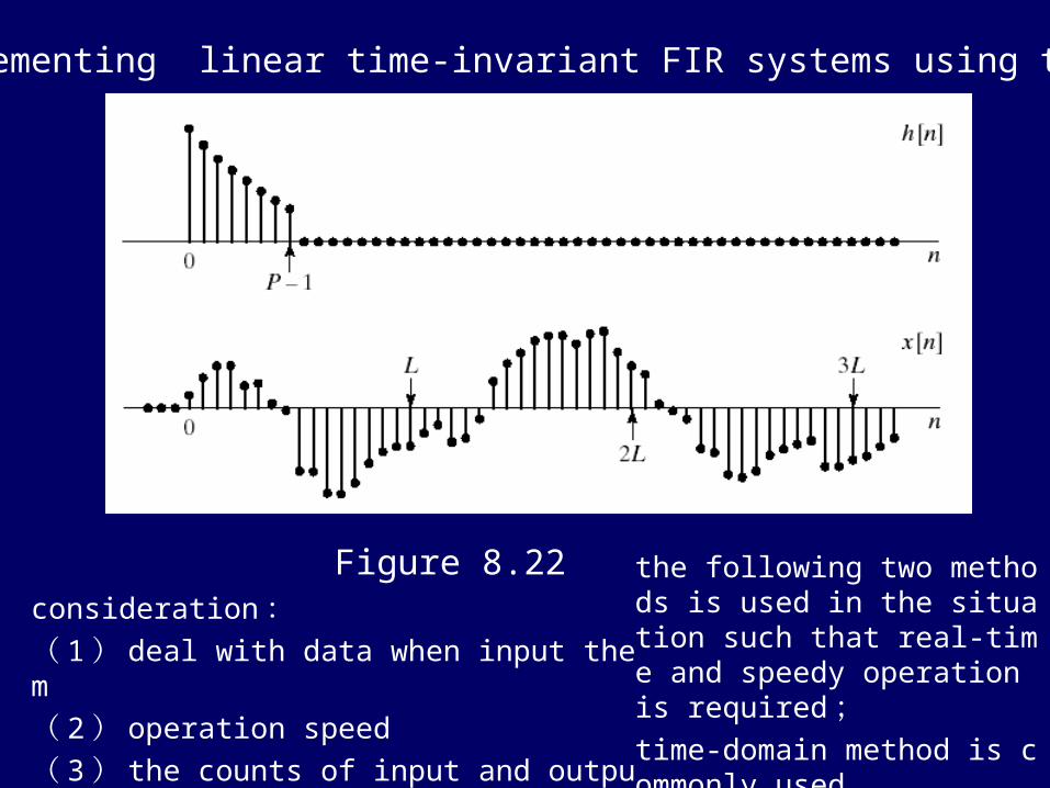
Figure 8.22

implementing linear time-invariant FIR systems using the DFT

consideration：（ 1） deal with data when input them

（ 2） operation speed

（ 3） the counts of input and output data are equal

the following two methods is used in the situation such that real-time and speedy operation is required；time-domain method is commonly used。

overlap-add method

(1)segment into sections of length L;

(2)fill 0 into and some section of , then do L+P-1 points FFT ;

(3) calculate

(4)add the points n=0…P-2 in to the last P-1 points in the former section y[n]，the output for this section is the points n=0…L-1

)(nh)(nx

)(nx

2,...0)}()({)( PLnkXkHIFFTny ，

)(ny

length of h[n] is P

P-1 points

2,...

...]3[]3[]2[0]1[0]0[0)(0

PLLn

hnxhhhny

2,..0...,]4[0]3[0

]2[]2[]1[]1[]0[][)(1

Pnhh

hnxhnxhnxny

2,...0],[][)( 212 Pnnynyny

Figure 8.24

overlap-save method

the length of h[n] is P

P-1 points

linear convolution

result

If do L+P-1 points DFT, then wipe off the first and last P-1 points in the result, respectively, output is the middle L-P+1 points。To guarantee the output is linear convolution result, the minimum points of DFT is L。

(1)segment into sections of length L, overlap P-1 points;

(2)fill 0 into and some section of , then do L points FFT ;

(3) calculate

(4) the output for this section is the L-P+1 points n=P-1,…L-1 of y[n]

)(nx

)(nh )(nx

1,...0)}()({)( LnkXkHIFFTny ，

Conclusion : use of DFT：（ 1） calculate spectral sample of signals

（ 2） calculate sample of frequency response of systems

（ 3） frequency-domain realization for FIR system

8.8 the discrete cosine transform(DCT)

10),2

)12(cos(][

2][

10),2

)12(cos(][

2][2

10),1

cos(][1

2][

10),1

cos(][1

2][1

1

0

1

0

1

0

1

0

NnN

nkkXc

Nnx

NkN

nknxc

NkXDCT

NnN

knkXcc

Nnx

NkN

knnxcc

NkXDCT

N

n

k

N

n

k

N

n

kn

N

n

nk

：

：

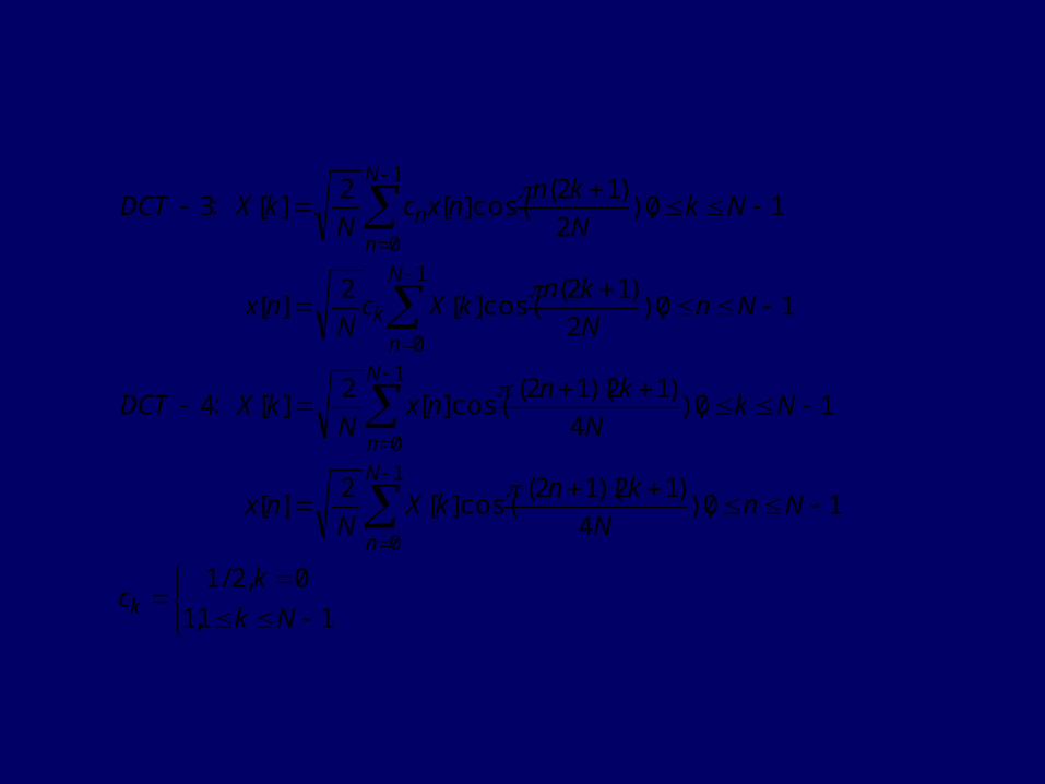
11,1

0,2/1

10),4

)12)(12(cos(][

2][

10),4

)12)(12(cos(][

2][4

10),2

)12(cos(][

2][

10),2

)12(cos(][

2][3

1

0

1

0

1

0

1

0

Nk

kc

NnN

knkX

Nnx

NkN

knnx

NkXDCT

NnN

knkXc

Nnx

NkN

knnxc

NkXDCT

k

N

n

N

n

N

n

k

N

n

n

：

：

-2 –1. 0. 1. 2. 3. 4. 5

-4 –3 -2-1 0. 1. 2. 3. 4. 5. 6. 7

DCT-1

DCT-2

-2 –1. 0. 1. 2. 3. 4. 5

-2 –1. 0. 1. 2. 3. 4. 5

-4 –3 -2-1 0. 1. 2. 3. 4. 5. 6. 7

-4 –3 -2-1 0. 1. 2. 3. 4. 5. 6. 7

symmetric and periodic extension of signal, then do DFS

and get DCT by taking the dominant period。

)2

/(][2

)2

)12(cos(][2

][][

]12[][][][

12,...],12[

1,...0],[][

2

2/2

1

0

2/2

1

0

)12(2

1

0

2

12

2

1

0

2

12

0

2

kkN

N

n

kN

N

n

nNkN

N

n

knN

N

Nn

knN

N

n

knN

N

n

knN

cN

kXW

N

knnxW

WnxWnx

WnNxWnxWnykY

NNnnNX

Nnnxny

DCT

relationship between 2N-poinsts DFT of extended sequence and N-points DCT o

f original sequence

Compare with DFT:energy compaction property

0 1 2 3 4 5 6 7

DCT

0 1 2 3 4 5 6 7

DFT

summary

8.1 representation of periodic sequences: the discrete fourier series

8.2 the fourier transform of periodic signals

8.3 properties of the discrete fourier series

8.4 fourier representation of finite-duration sequences:Definition of the discrete fourier transform

8.5 sampling the fourier transform (point of sampling)

8.6 properties of the fourier transform

8.7 linear convolution using the discrete fourier transform

8.8 the discrete cosine transform (DCT)

requirements：definition, calculation and properties of DFS;

derivation of definition of DFT： DFS or spectral sampling;

concepts of spectral sampling, ， time-domain periodic extension;

properties of DFT： linearity、 circular shift , symmetry, circular convolution、 paswal’s theory;

relationship between linear and circular convolution;

derivation of definition DCT and comparison with DFT.

key and difficulty： spectral sampling and properties of DFT

exercises

8.26 8.29 8.39 8.45 8.49