830 IEEE TRANSACTIONS ON CONTROL SYSTEMS …people.bu.edu/cgc/Published/TCSTprint_03_16.pdf830 IEEE TRANSACTIONS ON CONTROL SYSTEMS TECHNOLOGY, VOL. 24, NO. 3, MAY 2016 Adaptive Quasi-Dynamic

830 IEEE TRANSACTIONS ON CONTROL SYSTEMS TECHNOLOGY, VOL. 24, NO. 3, MAY 2016

Adaptive Quasi-Dynamic Traffic Light ControlJulia L. Fleck, Christos G. Cassandras, Fellow, IEEE, and Yanfeng Geng, Student Member, IEEE

Abstract— We consider the traffic light control problem fora single intersection modeled as a stochastic hybrid system.We study a quasi-dynamic policy based on partial state infor-mation defined by detecting whether vehicle backlogs are aboveor below certain thresholds. The policy is parameterized bygreen and red cycle lengths as well as the road contentthresholds. Using infinitesimal perturbation analysis, we deriveonline gradient estimators of a cost metric with respect to thecontrollable light cycles and threshold parameters and use theseestimators to iteratively adjust all the controllable parametersthrough an online gradient-based algorithm so as to improvethe overall system performance under various traffic conditions.The results obtained by applying this methodology to a simulatedurban setting are also included.

Index Terms— Optimization, perturbation analysis, stochastichybrid systems (SHSs), traffic light control (TLC), traffic signalsystems, transportation systems.

I. INTRODUCTION

THE traffic light control (TLC) problem consists inadjusting green and red signal settings in order to

control the traffic flow through an intersection and, moregenerally, through a set of intersections and traffic lightsin an urban roadway network. The ultimate objective is tominimize congestion (hence delays experienced by drivers andresulting reductions in fuel usage and pollution) at a particularintersection, as well as an entire area consisting of multipleintersections. There are two types of control strategies forthe TLC problem in the literature: fixed-time and traffic-responsive strategies. In the former, several timing planscovering different traffic intensity scenarios are periodicallyinterchanged; for example, the urban traffic controlsystem [48], TRANSYT [37], and MAXBAND [30] allmake use of historical traffic flow data to determine lightcycles offline and cannot adapt in real time to evolving trafficconditions. Traffic-responsive strategies address this limitationby making use of current traffic information to determine opti-mal signal settings online. They employ algorithms that adjusta signal’s phase length and phase sequences so as to minimize

Manuscript received December 9, 2014; revised May 8, 2015; acceptedJuly 27, 2015. Date of publication August 28, 2015; date of current versionApril 18, 2016. Manuscript received in final form August 4, 2015. Thiswork was supported in part by the National Science Foundation underGrant CNS-1239021 and Grant IIP-1430145, in part by the Air ForceOffice of Scientific Research under Grant FA9550-12-1-0113, in part by theOffice of Naval Research under Grant N00014-09-1-1051, and in part bythe Cyprus Research Promotion Foundation through the New InfrastructureProject/Strategic/0308/26. Recommended by Associate Editor F. Basile.

J. L. Fleck and C. G. Cassandras are with the Division of Systems Engi-neering, Center for Information and Systems Engineering, Boston University,Brookline, MA 02446 USA (e-mail: [email protected]; [email protected]).

Y. Geng is with Amazon, Boston, MA 02138 USA (e-mail:[email protected]).

Color versions of one or more of the figures in this paper are availableonline at http://ieeexplore.ieee.org.

Digital Object Identifier 10.1109/TCST.2015.2468181

delays and reduce the number of stops, requiring transitsurveillance, typically implemented using pavement loopdetectors, in order to adjust signal timing in real time.SCATS [32] and SCOOT [29] are two well-known examplesof traffic control systems that implement traffic-responsivestrategies.

Recent technological developments, which exploit theability to collect traffic data in real time, have made it possiblefor new methods to be applied to the TLC problem, resulting insystems such as OPAC [20], PRODYN [26], RHODES [39],and ACS Lite [40]. Leveraging the fact that TLC isfundamentally a form of scheduling for systems operatingthrough simple switching control actions, numerous solutionalgorithms have been proposed and we briefly review someof them next. Fuzzy logic was first used in [34] for a singleintersection without turning traffic, and in [8], a fuzzy logiccontroller was presented capable of coping with traffic con-gestion over multiple intersections. Expert systems were usedin [15], [16], and [46] to design TLC systems with featuressuch as distributed control and an ability to deal withcongested traffic. Evolutionary algorithms such as geneticalgorithms [31], swarm optimization algorithms [10], [11],and ant algorithms [47] have also been proposed. Severalapproaches using artificial neural networks have been reportedin [12], [27], and [41]. Reinforcement learning has also beenused for TLC within a Markov decision process (MDP)framework, as reported in [1], [3], [39], and [46].A discrete-time stationary MDP framework was also usedin [52] to develop an adaptive control model of a networkof signalized intersections. A game theoretic approach wasapplied to a finite controlled Markov chain model in [2].In [35], a decision tree model was used with a rolling horizondynamic programming approach, while a multiobjectivemixed integer linear programming formulation was proposedin [14]. Optimal TLC was also stated as a special case ofan extended linear complementarity problem in [38] andformulated as a hybrid system optimization problem in [53].Robust optimization methods that take into account uncertaintraffic flows have also been proposed. For example, in [42],a semidefinite programming routine for model predictivecontrol is used; in [44], a robust optimal signal controlproblem is formulated as a linear program; in [51], signaltimings were determined so as to minimize the mean delayper vehicle under daily traffic flow variations.

The aforementioned methods for real-time adaptive trafficcontrol must address two main issues: 1) the developmentof a mathematical model for a stochastic and highly non-linear traffic system and 2) the design of appropriate controllaws. Although most existing adaptive signal control strategiesimplicitly recognize that variations in traffic conditions are

1063-6536 © 2015 IEEE. Personal use is permitted, but republication/redistribution requires IEEE permission.See http://www.ieee.org/publications_standards/publications/rights/index.html for more information.

FLECK et al.: ADAPTIVE QUASI-DYNAMIC TLC 831

caused by random processes, they frequently resort to usingdeterministic models, which significantly simplify the descrip-tion of vehicle flow. In addition, heuristic control strategiesare also commonly employed for TLC without an embeddedtraffic flow model, as in the case of artificial intelligencetechniques, which rely on historical data. Such applicationsare, as a result, better suited for traffic systems in steadystate, which is in fact seldom attained. Stochastic controlapproaches address this limitation by explicitly accountingfor the random variations in traffic flow, typically within anMDP framework, which requires specific probabilistic models.Furthermore, many of these approaches, such as those basedon dynamic programming, are computationally inefficient,thus not immediately amenable to online implementations.In contrast to the above, perturbation analysis techniques [5]are entirely data driven and allow for stochastic control withno explicit traffic model required. They have proven to beadaptive and easily implementable online.

Perturbation analysis was used in [18] and [25] basedon modeling a traffic light intersection as a stochasticdiscrete event system (DES). An infinitesimal perturbationanalysis (IPA) approach, using a stochastic flow model (SFM)to represent the queue content dynamics of roads at anintersection, was presented in [33]. IPA was also applied withrespect to controllable green and red phase times for a singleisolated intersection in [22] and for multiple intersectionsin [21] and [24]. Modeling traffic flow through an intersectioncontrolled by switching traffic lights as an SFM convenientlycaptures the system’s inherent hybrid nature: while trafficlight switches exhibit event-driven dynamics, the flow ofvehicles through an intersection is best represented usingtime-driven dynamics. Moreover, traffic flow rates need not berestricted to take on deterministic values, but may be treatedas stochastic processes [6], which are suited to representthe continuous random variations in traffic conditions. Usingthe general IPA theory for stochastic hybrid systems (SHSs)in [7] and [45], online gradients of performance measures maybe estimated with respect to several controllable parameterswith only minor technical conditions imposed on the randomprocesses that define input and output flows at an intersection.Note that the purpose of IPA is not to estimate performancemeasures themselves, but only their gradients, whichmay be subsequently incorporated into standard gradient-based algorithms in order to effectively control parameters ofinterest. In particular, we stress that the IPA estimates obtaineddo not depend on any modeling assumptions for randomtraffic processes and involve only directly observable data.

There are several advantages associated with the use ofIPA for the TLC problem:

1) IPA estimates have been shown to be unbiased undervery mild conditions [50].

2) IPA estimators are robust with respect to the stochasticprocesses used in our model [4]. This is particularlyrelevant in the context of TLC, since the vehicle arrivaland departure processes are intrinsically random.

3) IPA is event driven and hence scalable in the number ofevents in the system (generally manageable), and doesnot explode with the space dimensionality.

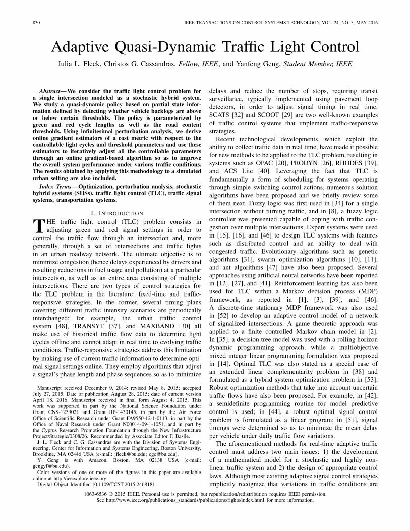
Fig. 1. Single traffic light intersection with two cross roads.

4) IPA possesses a decomposability property [4],i.e., IPA state derivatives become memoryless aftercertain events take place.

5) The IPA methodology can be easily implemented online,allowing us to take advantage of directly observed data.

In contrast to [9], [19], and [28] where the adjustment oflight phases did not make use of real-time state information,a quasi-dynamic control setting was proposed in [23] inwhich partial state information is used to adjust the greenand red light times conditioned upon a given queue contentthreshold being reached. A complementary approach, inwhich a quasi-dynamic policy is used to control the thresholdparameters while assuming fixed phase times, is presentedin [17]. Building upon these results, here we derive IPAperformance measure estimators necessary to simultaneouslyoptimize phase times and queue content threshold valueswithin a quasi-dynamic control setting.

From a practical perspective, the goal of this paper is topresent the basic IPA techniques applied to efficient adaptivetraffic signal control using real-time information. Therefore,we introduce the relevant concepts related to an IPA-basedTLC system ignoring several traffic engineering details whichwe believe can be readily incorporated into the proposedcontroller, as further discussed in Section III-C.

The remainder of this paper is organized as follows.In Section II, we formulate the TLC problem for a singleintersection and present the modeling framework usedthroughout our analysis for controlling green and red phaselengths and vehicle queue thresholds. Section III details thederivation of an IPA estimator for the cost function gradientwith respect to a controllable parameter vector defined bythe green and red phase lengths and threshold parameters.The IPA estimator is then incorporated into a gradient-basedoptimization algorithm, and a number of implementationissues are discussed. We include the simulation resultsin Section IV, showing how the proposed quasi-dynamiccontrol offers considerable improvement over prior results.Finally, we conclude and discuss future work in Section V.

II. PROBLEM FORMULATION

We consider a single intersection, as shown in Fig. 1. Forsimplicity, left-turn and right-turn traffic flows are not consid-ered and yellow light times are implicitly accounted for withina red phase. This system involves a number of stochasticprocesses that are all defined on a common probability space(�, F, P). Each road is modeled as a queue with a randomarrival flow process {αn(t)}, n = 1, 2, where αn(t) is theinstantaneous vehicle arrival rate at time t . When the traffic


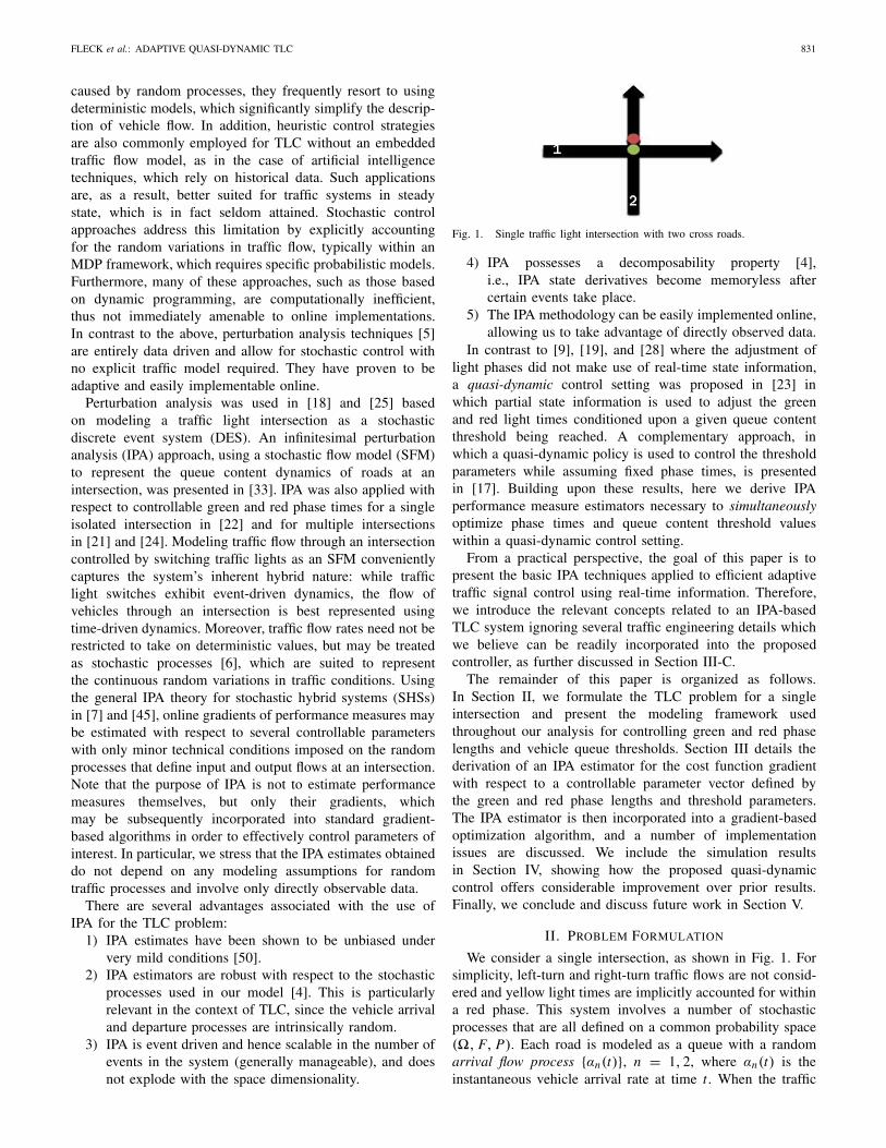
Fig. 2. State-space representation.

light corresponding to road n is GREEN, the departure flowprocess is denoted by {βn(t)}, n = 1, 2. We define a statevector x(t) = [x1(t), x2(t)], where xn(t) ∈ R

+ is the flowcontent of queue i , and assign to each queue n a guaran-teed minimum GREEN light length θn,min and a maximumlength θn,max. For each queue n, we also define a clock statevariable zn(t), n = 1, 2, which measures the time since the lastswitch from RED to GREEN of the traffic light for queue n,so that zn(t) ∈ [0, θn,max]. Setting z(t) = [z1(t), z2(t)], thecomplete system state vector is [x(t), z(t)].

A dynamic controller is one that makes full use of thestate information z(t) and x(t). Obviously, z(t) is thecontroller’s known internal state, but the queue content stateis generally not instantaneously observable. We assume,however, that it is partially observable. Specifically, we canonly observe whether xn(t) is below or above some thresholdsn , i = 1, 2. This is consistent with actual traffic systemswhere sensors, e.g., inductive loop detectors, are installed ateach road near the intersection. Moreover, there is a growingtrend toward exploiting connected vehicle technology toinfer state variables xn(t) from data (e.g., location andspeed) wirelessly exchanged through vehicle-to-vehicle orvehicle-to-infrastructure communication [13]. In this context,we shall define a quasi-dynamic controller where thecontrollable parameter vector of interest is given by

υ = [θ1,min, θ1,max, θ2,min, θ2,max, s1, s2] (1)

where θn,min ≥ 0 and θn,max > θn,min were defined aboveand sn ∈ �+ is a queue content threshold value forroad n = 1, 2 whose precise function is explained next.The notation x(υ, t) = [x1(υ, t), x2(υ, t)] is used to stress thedependence of the state on the six controllable parameters.However, for notational simplicity, we will henceforthwrite x(t) when no confusion arises; the same applies to z(t).

Let us now partition the queue content state space into thefollowing four regions (as shown in Fig. 2):

X0 = {(x1, x2) : x1(t) < s1, x2(t) < s2}X1 = {(x1, x2) : x1(t) < s1, x2(t) ≥ s2}X2 = {(x1, x2) : x1(t) ≥ s1, x2(t) < s2}X3 = {(x1, x2) : x1(t) ≥ s1, x2(t) ≥ s2}.

At any time t , the feasible control set for the traffic lightcontroller is U = {1, 2} and the control is defined as

u(x(t), z(t))≡{

1, i.e., set road 1 GREEN, road 2 RED2, i.e., set road 2 GREEN, road 1 RED.

(2)

We define a quasi-dynamic controller of the formu(X (t), z(t)), with X (t) ∈ {X0, X1, X2, X3}, as follows:

for X (t) ∈ {X0, X3}

u(z(t)) ={

1, if z1(t) ∈ (0, θ1,max) and z2(t) = 0

2, otherwise(3)

for X (t) = X1

u(z(t)) ={

1, if z1(t) ∈ (0, θ1,min) and z2(t) = 0

2, otherwise(4)

for X (t) = X2

u(z(t)) ={

2, if z2(t) ∈ (0, θ2,min) and z1(t) = 0

1, otherwise.(5)

This is a simple form of hysteresis control to ensure thatthe nth traffic flow always receives a minimum GREEN lighttime θn,min. Clearly, the GREEN phase may be dynamicallyinterrupted anytime after θn,min based on the partial statefeedback provided through X (t). For instance, if a transitioninto X1 occurs while u(X (t), z(t)) = 1 and z1(t) > θ1,min,then the light switches from GREEN to RED for road 1 inorder to accommodate an increasing backlog x2(t) ≥ s2 atroad 2. For notational simplicity, we will write u(t) when noconfusion arises, as we do with x(t) and z(t).

We can now write the dynamics of the state variables xn(t)and zn(t), starting with the observation that the departure flowprocess βn(t) on road n is given by

βn(t) =

⎧⎪⎨⎪⎩

hn(X (t), z(t), t), if xn(t) > 0 and u(t) = n

αn(t), if xn(t) = 0 and u(t) = n

0, otherwise(6)

where hn(X (t), z(t), t) [subsequently also written as hn(t)]is the instantaneous vehicle departure rate at time t , whichgenerally depends on the specifics of the intersection andvehicle behavior. Then, adopting the notation n to denote theindex of the road perpendicular to road n = 1, 2, we have

·xn(t) =

⎧⎪⎨⎪⎩

αn(t), if zn(t)=0

0, if xn(t)=0 and αn(t)≤hn(t)

αn(t) − βn(t), otherwise

(7)

·zn(t) =

{1, if zn(t) = 0

0, otherwise(8)

zn(t+) = 0

if zn(t) = θn,max

or zn(t) = θn,min, xn(t) < sn, xn(t) ≥ sn

or zn(t) > θn,min, xn(t−) > sn, xn(t

+) = sn, xn(t) ≥ sn

or zn(t) > θn,min, xn(t) < sn, xn(t−) < sn, xn(t

+) = sn.

Observe that zn(t) is discontinuous in t when the light switchesfrom GREEN to RED on road n, since at this point, theGREEN cycle clock is reset to zero.

Thus, the traffic light intersection in Fig. 1 can be viewedas a hybrid system in which the time-driven dynamics are


Fig. 3. SHA under quasi-dynamic control.

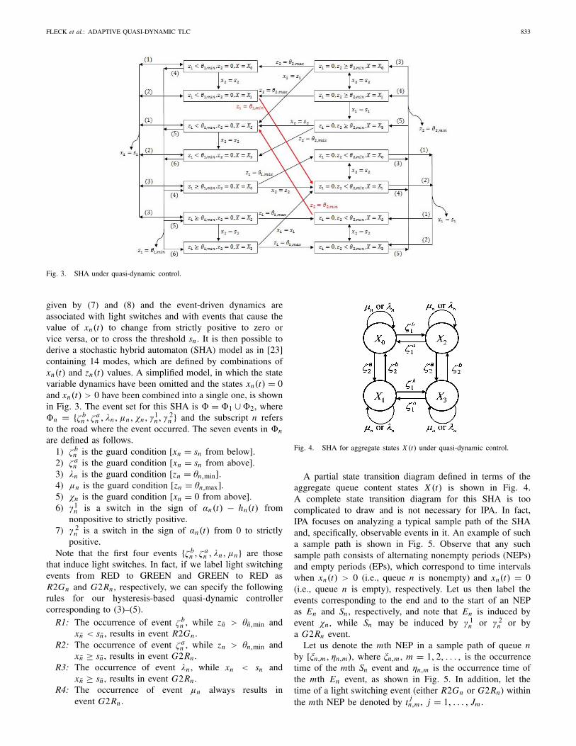
given by (7) and (8) and the event-driven dynamics areassociated with light switches and with events that cause thevalue of xn(t) to change from strictly positive to zero orvice versa, or to cross the threshold sn . It is then possible toderive a stochastic hybrid automaton (SHA) model as in [23]containing 14 modes, which are defined by combinations ofxn(t) and zn(t) values. A simplified model, in which the statevariable dynamics have been omitted and the states xn(t) = 0and xn(t) > 0 have been combined into a single one, is shownin Fig. 3. The event set for this SHA is � = �1 ∪ �2, where�n = {ζ b

n , ζ an , λn, μn, χn, γ

1n, γ 2

n } and the subscript n refersto the road where the event occurred. The seven events in �n

are defined as follows.1) ζ b

n is the guard condition [xn = sn from below].2) ζ a

n is the guard condition [xn = sn from above].3) λn is the guard condition [zn = θn,min].4) μn is the guard condition [zn = θn,max].5) χn is the guard condition [xn = 0 from above].6) γ1

n is a switch in the sign of αn(t) − hn(t) fromnonpositive to strictly positive.

7) γ 2n is a switch in the sign of αn(t) from 0 to strictly

positive.Note that the first four events {ζ b

n , ζ an , λn, μn} are those

that induce light switches. In fact, if we label light switchingevents from RED to GREEN and GREEN to RED asR2Gn and G2Rn , respectively, we can specify the followingrules for our hysteresis-based quasi-dynamic controllercorresponding to (3)–(5).

R1: The occurrence of event ζ bn , while zn > θn,min and

xn < sn , results in event R2Gn .R2: The occurrence of event ζ a

n , while zn > θn,min andxn ≥ sn , results in event G2Rn .

R3: The occurrence of event λn , while xn < sn andxn ≥ sn , results in event G2Rn .

R4: The occurrence of event μn always results inevent G2Rn .

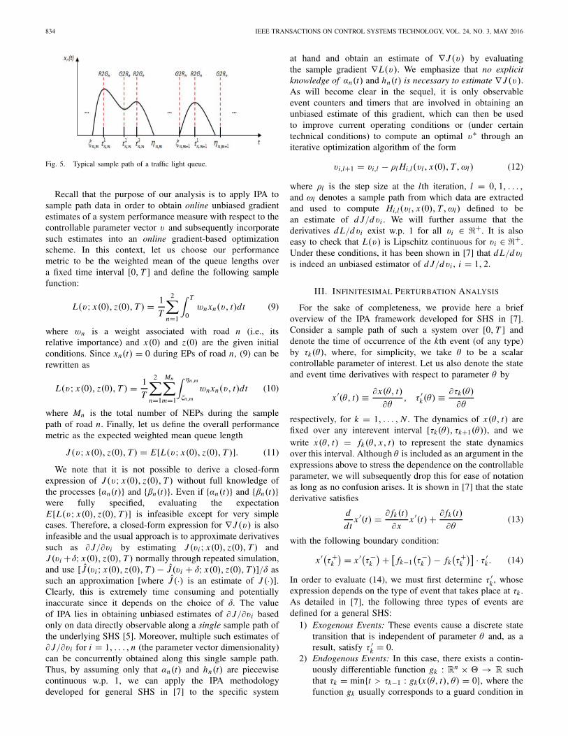
Fig. 4. SHA for aggregate states X (t) under quasi-dynamic control.

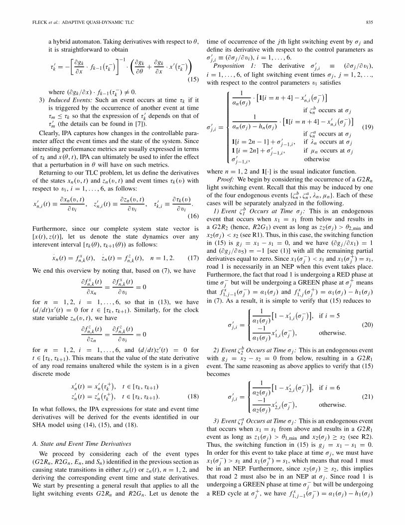
A partial state transition diagram defined in terms of theaggregate queue content states X (t) is shown in Fig. 4.A complete state transition diagram for this SHA is toocomplicated to draw and is not necessary for IPA. In fact,IPA focuses on analyzing a typical sample path of the SHAand, specifically, observable events in it. An example of sucha sample path is shown in Fig. 5. Observe that any suchsample path consists of alternating nonempty periods (NEPs)and empty periods (EPs), which correspond to time intervalswhen xn(t) > 0 (i.e., queue n is nonempty) and xn(t) = 0(i.e., queue n is empty), respectively. Let us then label theevents corresponding to the end and to the start of an NEPas En and Sn , respectively, and note that En is induced byevent χn , while Sn may be induced by γ 1

n or γ 2n or by

a G2Rn event.Let us denote the mth NEP in a sample path of queue n

by [ξn,m , ηn,m), where ξn,m , m = 1, 2, . . . , is the occurrencetime of the mth Sn event and ηn,m is the occurrence time ofthe mth En event, as shown in Fig. 5. In addition, let thetime of a light switching event (either R2Gn or G2Rn) withinthe mth NEP be denoted by t j

n,m , j = 1, . . . , Jm .


Fig. 5. Typical sample path of a traffic light queue.

Recall that the purpose of our analysis is to apply IPA tosample path data in order to obtain online unbiased gradientestimates of a system performance measure with respect to thecontrollable parameter vector υ and subsequently incorporatesuch estimates into an online gradient-based optimizationscheme. In this context, let us choose our performancemetric to be the weighted mean of the queue lengths overa fixed time interval [0, T ] and define the following samplefunction:

L(υ; x(0), z(0), T ) = 1

T

2∑n=1

∫ T

0wn xn(υ, t)dt (9)

where wn is a weight associated with road n (i.e., itsrelative importance) and x(0) and z(0) are the given initialconditions. Since xn(t) = 0 during EPs of road n, (9) can berewritten as

L(υ; x(0), z(0), T ) = 1

T

2∑n=1

Mn∑m=1

∫ ηn,m

ξn,m

wnxn(υ, t)dt (10)

where Mn is the total number of NEPs during the samplepath of road n. Finally, let us define the overall performancemetric as the expected weighted mean queue length

J (υ; x(0), z(0), T ) = E[L(υ; x(0), z(0), T )]. (11)

We note that it is not possible to derive a closed-formexpression of J (υ; x(0), z(0), T ) without full knowledge ofthe processes {αn(t)} and {βn(t)}. Even if {αn(t)} and {βn(t)}were fully specified, evaluating the expectationE[L(υ; x(0), z(0), T )] is infeasible except for very simplecases. Therefore, a closed-form expression for ∇ J (υ) is alsoinfeasible and the usual approach is to approximate derivativessuch as ∂ J/∂vi by estimating J (vi ; x(0), z(0), T ) andJ (vi +δ; x(0), z(0), T ) normally through repeated simulation,and use [ J(vi ; x(0), z(0), T ) − J (vi + δ; x(0), z(0), T )]/δ assuch an approximation [where J (·) is an estimate of J (·)].Clearly, this is extremely time consuming and potentiallyinaccurate since it depends on the choice of δ. The valueof IPA lies in obtaining unbiased estimates of ∂ J/∂vi basedonly on data directly observable along a single sample path ofthe underlying SHS [5]. Moreover, multiple such estimates of∂ J/∂vi for i = 1, . . . , n (the parameter vector dimensionality)can be concurrently obtained along this single sample path.Thus, by assuming only that αn(t) and hn(t) are piecewisecontinuous w.p. 1, we can apply the IPA methodologydeveloped for general SHS in [7] to the specific system

at hand and obtain an estimate of ∇ J (υ) by evaluatingthe sample gradient ∇L(υ). We emphasize that no explicitknowledge of αn(t) and hn(t) is necessary to estimate ∇ J (υ).As will become clear in the sequel, it is only observableevent counters and timers that are involved in obtaining anunbiased estimate of this gradient, which can then be usedto improve current operating conditions or (under certaintechnical conditions) to compute an optimal υ∗ through aniterative optimization algorithm of the form

υi,l+1 = υi,l − ρl Hi,l(υl , x(0), T, ωl ) (12)

where ρl is the step size at the lth iteration, l = 0, 1, . . . ,and ωl denotes a sample path from which data are extractedand used to compute Hi,l(υl, x(0), T, ωl ) defined to bean estimate of d J/dυi . We will further assume that thederivatives d L/dυi exist w.p. 1 for all υi ∈ �+. It is alsoeasy to check that L(υ) is Lipschitz continuous for υi ∈ �+.Under these conditions, it has been shown in [7] that d L/dυi

is indeed an unbiased estimator of d J/dυi , i = 1, 2.

III. INFINITESIMAL PERTURBATION ANALYSIS

For the sake of completeness, we provide here a briefoverview of the IPA framework developed for SHS in [7].Consider a sample path of such a system over [0, T ] anddenote the time of occurrence of the kth event (of any type)by τk(θ), where, for simplicity, we take θ to be a scalarcontrollable parameter of interest. Let us also denote the stateand event time derivatives with respect to parameter θ by

x ′(θ, t) ≡ ∂x(θ, t)

∂θ, τ ′

k(θ) ≡ ∂τk(θ)

∂θ

respectively, for k = 1, . . . , N . The dynamics of x(θ, t) arefixed over any interevent interval [τk(θ), τk+1(θ)), and wewrite

·x(θ, t) = fk(θ, x, t) to represent the state dynamics

over this interval. Although θ is included as an argument in theexpressions above to stress the dependence on the controllableparameter, we will subsequently drop this for ease of notationas long as no confusion arises. It is shown in [7] that the statederivative satisfies

d

dtx ′(t) = ∂ fk(t)

∂xx ′(t) + ∂ fk(t)

∂θ(13)

with the following boundary condition:x ′(τ+

k

) = x ′(τ−k

) + [fk−1

(τ−

k

) − fk(τ+

k

)] · τ ′k . (14)

In order to evaluate (14), we must first determine τ ′k , whose

expression depends on the type of event that takes place at τk .As detailed in [7], the following three types of events aredefined for a general SHS:

1) Exogenous Events: These events cause a discrete statetransition that is independent of parameter θ and, as aresult, satisfy τ ′

k = 0.2) Endogenous Events: In this case, there exists a contin-

uously differentiable function gk : Rn × � → R such

that τk = min{t > τk−1 : gk(x(θ, t), θ) = 0}, where thefunction gk usually corresponds to a guard condition in


a hybrid automaton. Taking derivatives with respect to θ ,it is straightforward to obtain

τ ′k = −

[∂gk

∂x· fk−1

(τ−

k

)]−1

·(

∂gk

∂θ+ ∂gk

∂x· x ′(τ−

k

))(15)

where (∂gk/∂x) · fk−1(τ−k ) �= 0.

3) Induced Events: Such an event occurs at time τk if itis triggered by the occurrence of another event at timeτm ≤ τk so that the expression of τ ′

k depends on that ofτ ′

m (the details can be found in [7]).

Clearly, IPA captures how changes in the controllable para-meter affect the event times and the state of the system. Sinceinteresting performance metrics are usually expressed in termsof τk and x(θ, t), IPA can ultimately be used to infer the effectthat a perturbation in θ will have on such metrics.

Returning to our TLC problem, let us define the derivativesof the states xn(υ, t) and zn(υ, t) and event times τk(υ) withrespect to υi , i = 1, . . . , 6, as follows:x ′

n,i (t) ≡ ∂xn(υ, t)

∂υi, z′

n,i (t) ≡ ∂zn(υ, t)

∂υi, τ ′

k,i ≡ ∂τk(υ)

∂υi.

(16)

Furthermore, since our complete system state vector is[x(t), z(t)], let us denote the state dynamics over anyinterevent interval [τk(θ), τk+1(θ)) as follows:

·xn(t) = f x

n,k(t),·zn(t) = f z

n,k(t), n = 1, 2. (17)

We end this overview by noting that, based on (7), we have

∂ f xn,k(t)

∂xn= ∂ f x

n,k(t)

∂υi= 0

for n = 1, 2, i = 1, . . . , 6, so that in (13), we have(d/dt)x ′(t) = 0 for t ∈ [τk, τk+1). Similarly, for the clockstate variable zn(υ, t), we have

∂ f zn,k(t)

∂zn= ∂ f z

n,k(t)

∂υi= 0

for n = 1, 2, i = 1, . . . , 6, and (d/dt)z′(t) = 0 fort ∈ [τk, τk+1). This means that the value of the state derivativeof any road remains unaltered while the system is in a givendiscrete mode

x ′n(t) = x ′

n

(τ+

k

), t ∈ [τk, τk+1)

z′n(t) = z′

n

(τ+

k

), t ∈ [τk, τk+1). (18)

In what follows, the IPA expressions for state and event timederivatives will be derived for the events identified in ourSHA model using (14), (15), and (18).

A. State and Event Time Derivatives

We proceed by considering each of the event types(G2Rn , R2Gn , En , and Sn) identified in the previous section ascausing state transitions in either xn(t) or zn(t), n = 1, 2, andderiving the corresponding event time and state derivatives.We start by presenting a general result that applies to all thelight switching events G2Rn and R2Gn . Let us denote the

time of occurrence of the j th light switching event by σ j anddefine its derivative with respect to the control parameters asσ ′

j,i ≡ (∂σ j/∂υi ), i = 1, . . . , 6.Proposition 1: The derivative σ ′

j,i ≡ (∂σ j/∂υi ),i = 1, . . . , 6, of light switching event times σ j , j = 1, 2, . . .,with respect to the control parameters υi satisfies

σ ′j,i =

⎧⎪⎪⎪⎪⎪⎪⎪⎪⎪⎪⎪⎪⎨⎪⎪⎪⎪⎪⎪⎪⎪⎪⎪⎪⎪⎩

1

αn(σ j )· [1[i = n + 4] − x ′

n,i

(σ−

j

)]if ζ b

n occurs at σ j1

αn(σ j ) − hn(σ j )· [1[i = n + 4] − x ′

n,i

(σ−

j

)]if ζ a

n occurs at σ j

1[i = 2n − 1] + σ ′j−1,i , if λn occurs at σ j

1 [i = 2n] + σ ′j−1,i , if μn occurs at σ j

σ ′j−1,i , otherwise

(19)

where n = 1, 2 and 1[·] is the usual indicator function.Proof: We begin by considering the occurrence of a G2Rn

light switching event. Recall that this may be induced by oneof the four endogenous events {ζ b

n , ζ an , λn, μn}. Each of these

cases will be separately analyzed in the following.1) Event ζ b

1 Occurs at Time σ j : This is an endogenousevent that occurs when x1 = s1 from below and results ina G2R2 (hence, R2G1) event as long as z2(σ j ) > θ2,min andx2(σ j ) < s2 (see R1). Thus, in this case, the switching functionin (15) is g j = x1 − s1 = 0, and we have (∂g j/∂x1) = 1and (∂g j/∂υ5) = −1 [see (1)] with all the remaining partialderivatives equal to zero. Since x1(σ

−j ) < s1 and x1(σ

+j ) = s1,

road 1 is necessarily in an NEP when this event takes place.Furthermore, the fact that road 1 is undergoing a RED phase attime σ−

j but will be undergoing a GREEN phase at σ+j means

that f x1, j−1(σ

−j ) = α1(σ j ) and f x

1, j (σ+j ) = α1(σ j ) − h1(σ j )

in (7). As a result, it is simple to verify that (15) reduces to

σ ′j,i =

⎧⎪⎪⎨⎪⎪⎩

1

α1(σ j )

[1 − x ′

1,i

(σ−

j

)], if i = 5

−1

α1(σ j )x ′

1,i

(σ−

j

), otherwise.

(20)

2) Event ζ b2 Occurs at Time σ j : This is an endogenous event

with g j = x2 − s2 = 0 from below, resulting in a G2R1event. The same reasoning as above applies to verify that (15)becomes

σ ′j,i =

⎧⎪⎪⎨⎪⎪⎩

1

α2(σ j )

[1 − x ′

2,i

(σ−

j

)], if i = 6

−1

α2(σ j )x ′

2,i

(σ−

j

), otherwise.

(21)

3) Event ζ a1 Occurs at Time σ j : This is an endogenous event

that occurs when x1 = s1 from above and results in a G2R1event as long as z1(σ j ) > θ1,min and x2(σ j ) ≥ s2 (see R2).Thus, the switching function in (15) is g j = x1 − s1 = 0.In order for this event to take place at time σ j , we must havex1(σ

−j ) > s1 and x1(σ

+j ) = s1, which means that road 1 must

be in an NEP. Furthermore, since x2(σ j ) ≥ s2, this impliesthat road 2 must also be in an NEP at σ j . Since road 1 isundergoing a GREEN phase at time σ−

j but will be undergoinga RED cycle at σ+

j , we have f x1, j−1(σ

−j ) = α1(σ j ) − h1(σ j )


and f x1, j (σ

+j ) = α1(σ j ) in (7). As a result, (15) can be seen

to become

σ ′j,i =

⎧⎪⎪⎨⎪⎪⎩

1

α1(σ j ) − h1(σ j )

[1 − x ′

1,i

(σ−

j

)], if i = 5

−1

α1(σ j ) − h1(σ j )x ′

1,i

(σ−

j

), otherwise.

(22)

4) Event ζ a2 Occurs at Time σ j : This is an endogenous

event with g j = x2 − s2 = 0 from above, resulting in a G2R2event. The same reasoning as above applies to verify that (15)reduces to

σ ′j,i =

⎧⎪⎪⎨⎪⎪⎩

1

α2(σ j ) − h2(σ j )

[1 − x ′

2,i

(σ−

j

)], if i = 6

−1

α2(σ j ) − h2(σ j )x ′

2,i

(σ−

j

), otherwise.

(23)

5) Event λ1 Occurs at Time σ j : This is an endogenous eventthat occurs when z1 = θ1,min and results in a G2R1 eventas long as x1(σ j ) < s1 and x2(σ j ) ≥ s2 (see R3). Thus, theswitching function in (15) is g j = z1−θ1,min = 0. Let τp < σ j

be the occurrence time of the last R2G1 event before λ1 takesplace at time σ j . It follows from (18) that (d/dt)z′

1,i (t) = 0,i = 1, . . . , 6, for t ∈ [τp, σ j ), and therefore z′

1,i (σ−j ) =

z′1,i (τ

+p ). Furthermore, the fact that road 1 is undergoing a

RED phase at time τ−p but will be undergoing a GREEN phase

at τ+p means that f z

1,p−1(τ−p ) = 0 and f z

1,p(τ+p ) = 1 in (8).

Let τr < τp also be the occurrence time of the last G2R1event before τp so that z′

1,i(τ−p ) = z′

1,i (τ+r ) by a similar

argument as above. Since z1(t) is reset to zero whenevera G2R1 event takes place, we have z′

1,i (τ+r ) = 0. As a

result, (14) can be easily seen to yield z′1,i (τ

+p ) = −τ ′

p,i ,i = 1, . . . , 6. Using a similar reasoning to the one appliedfor determining the change in state dynamics due to an R2G1event at τp, it is simple to verify that f z

1, j−1(σ−j ) = 1 and

f z1, j (σ

+j ) = 0. By substituting these expressions into (15) and

recalling that τp = σ j−1, we obtain

σ ′j,i =

{1 + σ ′

j−1,1, if i = 1

σ ′j−1,1, otherwise.

(24)

6) Event λ2 Occurs at Time σ j : This is an endogenous eventwith g j = z2 − θ2,min = 0, resulting in a G2R2 event. Let τr

be the time of occurrence of the last G2R1 event before λ2takes place at time σ j . The same reasoning as above appliesto verify that z′

2,i (σ−j ) = z′

2,i (τ+r ), i = 1, . . . , 6. Furthermore,

since light switches are coupled, road 2 is undergoing a REDphase at time τ−

r but will be undergoing a GREEN phaseat τ+

r so that f z2,r−1(τ

−r ) = 0 and f z

2,r (τ+r ) = 1. As a result,

(14) yields z′2,i (τ

+r ) = −τ ′

r,i . By substituting these expressionsinto (15) and recalling that τp = σ j−1, we obtain

σ ′j,i =

{1 + σ ′

j−1,1, if i = 3


(25)

7) Event μ1 Occurs at Time σ j : This is an endogenousevent that occurs when z1 = θ1,max and always results in aG2R1 event (see R3). Thus, the switching function in (15) is

g j = z1−θ1,max = 0. The same reasoning as in Case 5 appliesto verify that (15) reduces to

σ ′j,i =

{1 + σ ′

j−1,1, if i = 2


(26)

8) Event μ2 Occurs at Time σ j : This is an endogenousevent with g j = z2 − θ2,max = 0, resulting in a G2R2 event.The same reasoning as in Case 6 applies to verify that (15)reduces to

σ ′j,i =

{1 + σ ′

j−1,1, if i = 4


(27)

We will use Proposition 1 in the following, where weconsider each of the event types (G2Rn , R2Gn , En , and Sn ).

1) Event G2Rn: The following two cases must be consid-ered:

a) G2Rn Occurs at τk While Road n Is Undergoing anNEP: In this case, the fact that xn(τ

−k ) > 0 implies

from (7) that fn,k−1(τ−k ) = αn(τk) − hn(τk).

In addition, since road n is undergoing aRED phase at time τ+

k , we must have thatf xn,k(τ

+k ) = αn(τk). It follows from (14) that:

x ′n,i

(τ+

k

) = x ′n,i

(τ−

k

) − hn(τk)τ′k,i

for n = 1, 2 and i = 1, . . . , 6.b) G2Rn Occurs at τk While Road n Is Undergoing

an EP: In this case, xn(τ−k ) = 0, so that from (7),

we have fn,k−1(τ−k ) = 0, and it is simple to verify

that

x ′n,i

(τ+

k

) = x ′n,i

(τ−

k

) − αn(τk)τ′k,i

for n = 1, 2 and i = 1, . . . , 6. Finally, if the kthevent corresponds to the j th occurrence of a lightswitching event, we have that τ ′

k,i = σ ′j,i for some

j = 1, 2, . . .. As a result, combining the two casesabove, we get, for n = 1, 2 and i = 1, . . . , 6

x ′n,i

(τ+

k

) = x ′n,i

(τ−

k

)−

{hn(τk)σ

′j,i , if xn(τk) > 0

αn(τk)σ′j,i , if xn(τk) = 0

(28)

where σ ′j,i is given by (19) in Proposition 1 with

σ j = τk .

2) Event R2Gn: Once again, the following two cases mustbe considered:

a) R2Gn Occurs at τk While Road n Is Undergoingan NEP: In this case, the fact that road n isundergoing a RED phase within an NEP at timeτ−

k means that f xn,k−1(τ

−k ) = αn(τk), and since it

will be undergoing a GREEN phase at time τ+k ,

we must have that f xn,k(τ

+k ) = αn(τk) − hn(τk).

It follows from (14) that:

x ′n,i

(τ+

k

) = x ′n,i

(τ−

k

) + hn(τk)τ′k,i

for n = 1, 2 and i = 1, . . . , 6.


b) R2Gn Occurs at τk While Road n Is Undergoingan EP: In this case, the fact that road n is emptywhile undergoing a RED phase at time τ−

k impliesthat f x

n,k−1(τ−k ) = αn(τk) with 0 < αn(τk) ≤

hn(τk), while f xn,k(τ

+k ) = 0 in (7), and it is simple

to verify that

x ′n,i

(τ+

k

) = x ′n,i

(τ−

k

) + αn(τk)τ′k,i

for n = 1, 2 and i = 1, . . . , 6. Combiningthese two cases, we get, for n = 1, 2 andi = 1, . . . , 6

x ′n,i

(τ+

k

) = x ′n,i

(τ−

k

)

+

⎧⎪⎨⎪⎩

αn(τk)σ′j,i , if xn(τk) = 0 and

0<αn(τk)≤hn(τk)

hn(τk)σ′j,i , otherwise

(29)

where again σ ′j,i is given by (19) in Proposition 1

with σ j = τk .

3) Event En: This event corresponds to the end of an NEPon road n and is induced by χn , i.e., an endogenousevent such that xn = 0 from above. Thus, the switchingfunction in (15) is gk = xn = 0. The fact that road nis in an NEP at time τ−

k implies that f xn,k−1(τ

−k ) =

αn(τk) − hn(τk), and it follows from (15) thatτ ′

k,i = −(x ′n,i (τ

−k )/αn(τk) − hn(τk)). Furthermore, since

road n is in an EP at time τ+k , we have that f x

n,k(τ+k ) = 0

and (14) reduces to x ′n,i (τ

+k ) = x ′

n,i (τ−k ) − x ′

n,i (τ−k ) and

we get

x ′n,i

(τ+

k

) = 0, n = 1, 2 and i = 1, . . . , 6. (30)

4) Event Sn: This event corresponds to the start of an NEPon road n and can be induced either by a G2Rn event,or γ 1

n or γ 2n . These three cases will be analyzed in the

following.a) Sn Is Induced by a G2Rn Event: Suppose this is the

start of the mth NEP on road n. This means that,during the preceding EP, which corresponds to thetime interval [ηn,m−1, ξn,m ), we have xn(t) = 0 fort ∈ [ηn,m−1, ξn,m ) and, consequently, x ′

n,i (t) = 0for t ∈ [ηn,m−1, ξn,m) and i = 1, . . . , 6. Therefore,x ′

n,i (η+n,m−1) = x ′

n,i (ξ−n,m) = 0, and since τk

corresponds to the time when the NEP starts onroad n (i.e., τk = ξn,m ), it follows that x ′

n,i (τ−k ) =

x ′n,i (ξ

−n,m) = 0. As a result, (28) can be easily seen

to yield, for n = 1, 2 and i = 1, . . . , 6

x ′n,i

(τ+

k

) = −αn(τk)τ′k,i . (31)

The value of τ ′k,i in (31) depends on the type

of event that induced G2Rn . If the kth eventcorresponds to the j th light switching event, thenτ ′

k,i = σ ′j,i , whose expression is given by (19).

Note, however, that event Sn cannot be inducedby ζ a

n because the occurrence of event ζ an is con-

ditioned upon road n being in an NEP, and such

a case is not possible here. As a result, the secondcase in (19) must be excluded.

b) Sn Is Induced by a γ 2n Event: Recall that γ 2

ncorresponds to a switch from αn(t) = 0 toαn(t) > 0 while road n is undergoing a REDphase, i.e., zn(t) = 0. Since this is an exogenousevent, τ ′

k,i = 0, i = 1, . . . , 6, and (14) reduces tox ′

n,i (τ+k ) = x ′

n,i (τ−k ). We know that the NEP starts

on road n at time τk , so that τk = ξn,m , and wehave shown that x ′

n,i (ξ−n,m) = x ′

n,i (η+n,m−1) = 0.

It thus follows that x ′n,i (τ

−k ) = x ′

n,i (ξ−n,m) = 0, so

that x ′n,i (τ

+k ) = 0, for n = 1, 2 and i = 1, . . . , 6.

c) Sn Is Induced by a γ 1n Event: Event γ 1

n correspondsto a switch from αn(t) − hn(t) ≤ 0 to αn(t) −hn(t) > 0 while road n is undergoing a GREENphase, i.e., zn(t) > 0. Since this is an exogenousevent, τ ′

k,i = 0, i = 1, . . . , 6, and the subsequentanalysis is similar to that of the previous case. As aresult, x ′

n,i (τ+k ) = 0, for n = 1, 2 and i = 1, . . . , 6.

This completes the derivation of all the state and event timederivatives required to apply IPA to our TLC problem; the wayin which the above derivatives are used to ultimately estimated J/dυi , i = 1, . . . , 6, will be detailed next.

B. Cost Derivatives

Returning to (10), recall that the IPA estimator consists ofthe gradient formed by the sample performance derivativesd L/dυi . The following theorem provides the completeIPA estimator.

Theorem 1: The IPA estimator, i.e., the gradient of L(υ)consisting of d L(υ)/dυi , i = 1, . . . , 6 is given by

d L(υ)

dυi= 1

T

2∑n=1

Mn∑m=1

wnd Ln,m(υ)

dυi

where

Ln,m(υ) =∫ ηn,m

ξn.m

xn(υ,t)dt

d Ln,m(υ)

dυi= x ′

n,i ((ξn.m )+) · (t1n,m − ξn.m

)+ x ′

n,i

((t

Jn,mn,m

)+) · (ηn,m − tJn,mn,m

)+

Jn,m∑j=2

x ′n,i

((t jn,m

)+) · (t jn,m − t j−1

n,m). (32)

Proof: From (10), we obtain

d L(υ)

dυi= 1

T

2∑n=1

Mn∑m=1

ηn,m∫ξn.m

wnx ′n,i (t)dt + 1

T

2∑n=1

Mn∑m=1

×[wnxn(ηn,m) · ∂ηn,m

∂υi− wn xn(ξn.m) · ∂ξn.m

∂υi

].

Since, by the definition of an NEP, road n is empty both at thestart and end of an NEP, we have xn(ξn,m) = xn(ηn,m) = 0.Furthermore, we have shown in (18) that x ′

n,i (t) is piecewiseconstant throughout an NEP and its value changes only


Algorithm 1 IPA Algorithm for Quasi-Dynamic TLC

at instants when events take place. This implies that wecan decompose each NEP into time intervals of the form[ξn.m , t1

n,m), [t1n,m, t2

n,m), . . . , [t Jn,mn,m , ηn,m ). Using the definition

of Ln,m(υ), (32) immediately follows.

C. Implementation Issues

It is clear from (32) that evaluating the IPA estimatorrequires knowledge of: 1) the event times ξn.m , ηn,m , andt jn,m and 2) the value of the state derivatives x ′

n,i (t) at event

times t = ξn.m , t = tJn,mn,m , and t = t j

n,m . The quantitiesin 1) are easily observed using timers whose start and endtimes are observable events. The state derivatives in 2) areobtained from the expressions derived in (28) and (31) forG2Rn light switching events, (29) for R2Gn light switchingevents, and x ′

n,i (τ+k ) = 0 for all other events occurring at

t = τk . Ultimately, these expressions depend on the valuesof the arrival and departure rates αn(t) and hn(t) at lightswitching event times only, which may be estimated throughsimple rate estimators.

As a result, it is straightforward to implement an algorithmfor updating the value of d L(υ)/dυi after each observedevent, as outlined in Algorithm 1. For conciseness, only theevents occurring on road 1 are shown (note that, since eventsγ 1

1 and γ 21 have a null effect on the state derivatives, it is not

necessary to check for their occurrence).We also point out that our IPA estimator is linear in the

number of events in the SFM, not in its states. This is acrucial observation because it implies that our approach scaleswith the number of traffic lights in a network of intercon-nected intersections. Another crucial observation is that theIPA estimator depends only on events that are observablein the actual intersection operating as a DES; for example,event χn is simply the condition [xn = 0 from above], i.e., anevent representing the fact that a road queue becomes empty.In other words, even though the IPA estimator is derived fromour SFM (7), (8), its actual implementation is entirely drivenby actually observed events in the real intersection.

Extending the proposed controller to incorporatebidirectional and left/right turn traffic is straightforward,requiring the addition of variables that capture associatedtraffic flows and of parameters for the green/red times andbacklog thresholds. The extension to multiple intersections isalso a direct one as shown in [24] and includes phenomenaarising when upstream traffic flow is blocked by a congestedneighboring intersection; in fact, IPA equations explicitlycapture such effects. However, our simple model (7), (8)will have to be enhanced to incorporate acceleration anddeceleration delays, as well as delays in vehicles reachinga downstream traffic light dependent on the length betweenadjacent intersections and the state of the associated queues.

We also point out that our traffic light controller does notassume a fixed cycle consisting of red and green phases, i.e.,setting T = R + G, where T is fixed. This a special case ofour model, which can be easily incorporated in our analysis asshown in [22] by simply constraining the red and green phasesto add up to T and treating T, if desired, as a controllableparameter. This allows us to study the coordination of multipletraffic lights in series and achieve the so-called green waveswhereby vehicles maximize their chance of encountering agreen light over several intersections in a row.

As already mentioned, the purpose of this paper is todemonstrate the advantages of quasi-dynamic TLC using IPAtechniques before expanding this effort to networks of urbanroadways and multidirectional traffic flows. It is for this reasonthat all the simulation results reported in the next sectionwere obtained based on a simple simulator we developed,as opposed to commercial traffic network simulators(e.g., VISSIM). As we extend this work to multipleintersections and include the additional features discussedabove, we will be incorporating our controllers to suchcommercial simulators.

We end with a conceptual comparison of our methodologywith some well-known approaches (e.g., Webster’s method [9],SIGSET, and SIGCAP [28]). Since these approaches are fixed-time strategies, they must rely on historical data to determineand preset signal timings, and therefore signal cycles cannot beautomatically adjusted to handle fluctuating vehicle flows [19].Our methodology, on the other hand, allows for the design offully actuated signals, whose settings can be changed onlineto account for random traffic variations. In fact, our IPAalgorithm can be implemented online and is thus capable ofprocessing real-time traffic data, while the algorithms thatresult from the aforementioned strategies must be solvedoffline using historical data. Finally, we stress that, althoughwe have not implemented the Webster, SIGSET, and SIGCAPalgorithms, a comparison of the simulation results obtainedthrough our methodology and those obtained using fixed-timestrategies is given in Table I.

IV. SIMULATION RESULTS

In what follows, we detail how an IPA-driven gradient-based optimization approach can simultaneously control thegreen and red light times and the queue content thresholdsfor a single traffic light intersection, which is modeled asa DES. Two sets of simulations were performed: one in which


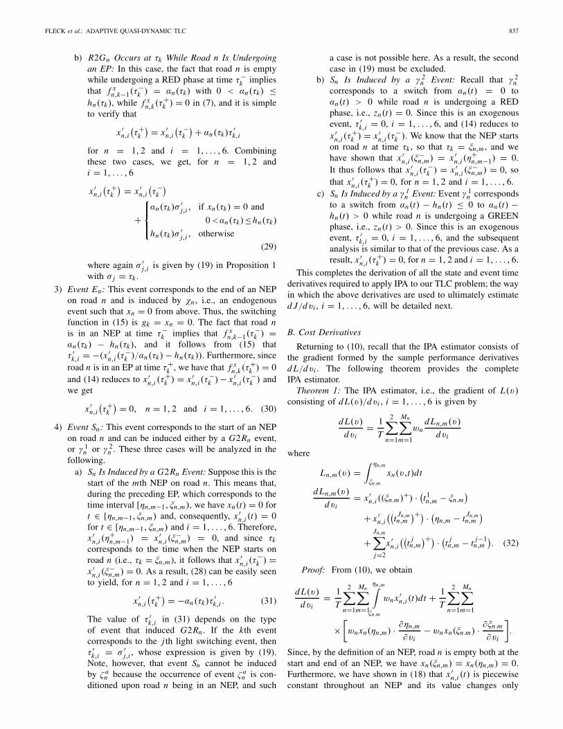
Fig. 6. Sample cost and parameter trajectories for 1/α = [1.7, 3].

TABLE I

OPTIMIZATION RESULTS FOR DIFFERENT TRAFFIC INTENSITIES

the same initial phase length/threshold setting was used fordifferent traffic intensities and another in which different start-ing points were used for the given values of traffic intensity.

In all our simulations, we assume that the vehicle arrivalprocess is Poisson with rate αn, n = 1, 2, and approximate thedeparture rate by a constant value hn(t) = H when road n isnonempty (this ignores acceleration effects and the interdepen-dence of queued vehicles). We nevertheless remind the readerthat our methodology applies independently of the distributionchosen to represent the arrival and departure processes, whichwe need only assume to be piecewise continuous w.p. 1.We estimate the values of the arrival rate at event times asαn(τk) = Na/tw, where Na corresponds to the number ofvehicle arrivals during a time window of size tw just before τk .We also note that we consider hn(t) = H throughout thenumerical simulations for simplicity; if the value of hn(t) werenot taken to be constant, we would simply need to estimate it atevent times only (exactly as we do for αn). Simulations of theintersection modeled as a pure DES are thus run to generatesample path data to which the IPA estimator is applied. In allthe results reported here, we set H = 1, wn = 1, and n = 1, 2,and measure the sample path length in between updates of thecontrollable parameter vector υ in terms of the number ofobserved light switches, which we choose to be N = 5000.

In our first set of simulations, the initial configuration waschosen to be θ0 = [15, 30, 15, 30] and s0 = [10, 10]. Table Ipresents the optimization results associated with differenttraffic intensities (denoted by 1/α), where θ∗

IPA and s∗IPA denote

the optimal phase lengths and threshold values, respectively,and J ∗

IPA is the cost associated with the optimal configuration.We also include here a comparison of the results generated byour methodology with those obtained when static control [22]is applied to determine the optimal phase lengths. This iscaptured by R(%) in Table I, the fractional cost reductionachieved by our method with respect to the static approach.The static controller defined in [22] adjusts the green lighttimes subject to some lower and upper bounds and determinesθ∗

static = [θ∗1 , θ∗

2 ], where θ∗1 (θ∗

2 , respectively) is the green phaselength that should be allotted to road 1 (road 2, respectively)so as to minimize the average queue content on both roads.The advantage of quasi-dynamically controlling the light cyclelengths and threshold values over a static IPA approach to theTLC problem was established in [17]. However, in [17], wemade use of a sequential optimization procedure, where firstthe optimal phase lengths were determined considering fixedthreshold values, and then the queue content thresholds wereoptimized. The magnitude of the cost reduction obtained usingthis approach varied in the range 38%–51%. We have foundthat performing a simultaneous optimization of both phaselengths and threshold values provides a cost reduction that isin most cases at least as high as the aforementioned sequentialapproach. Indeed, for 1/α = [1.7, 3], sequential optimizationyielded a 38% cost reduction, while our simultaneous opti-mization method allowed for a reduction of 46%, and for1/α = [2, 3], both approaches resulted in a comparable overallcost, which was 47% lower than the one obtained under staticcontrol for the simultaneous optimization and 51% lower in thecase of sequential optimization. Moreover, our methodologyconsistently yields results in which the traffic buildup at theintersection is approximately half the size of the one understatic control.

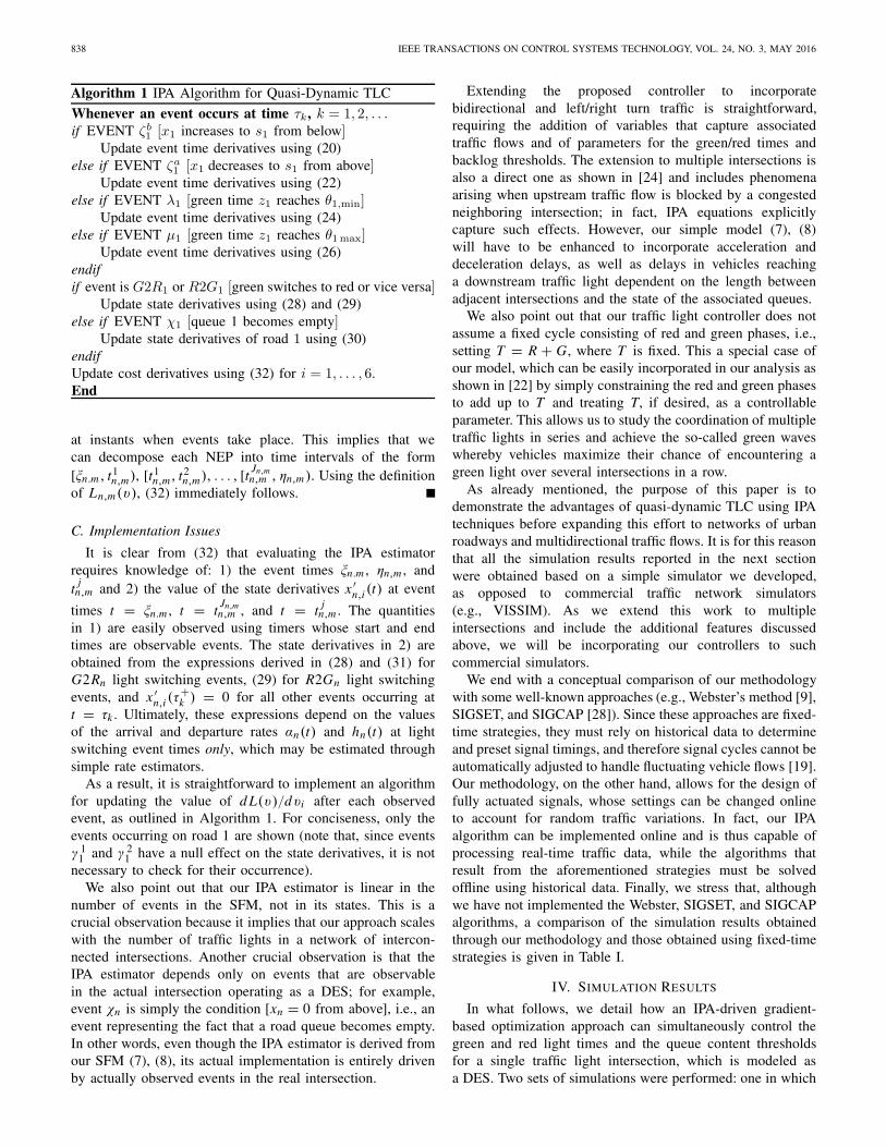
The convergence behavior of the cost and the control-lable phase lengths and threshold parameters are shownin Figs. 6 and 7. The left plot of Figs. 6 and 7 shows theaverage cost, which in this paper corresponds to the weightedmean of the queue length of both roads, while the middle and


Fig. 7. Sample cost and parameter trajectories for 1/α = [2, 6].TABLE II

CONVERGENCE RESULTS FOR DIFFERENT INITIAL CONFIGURATIONS

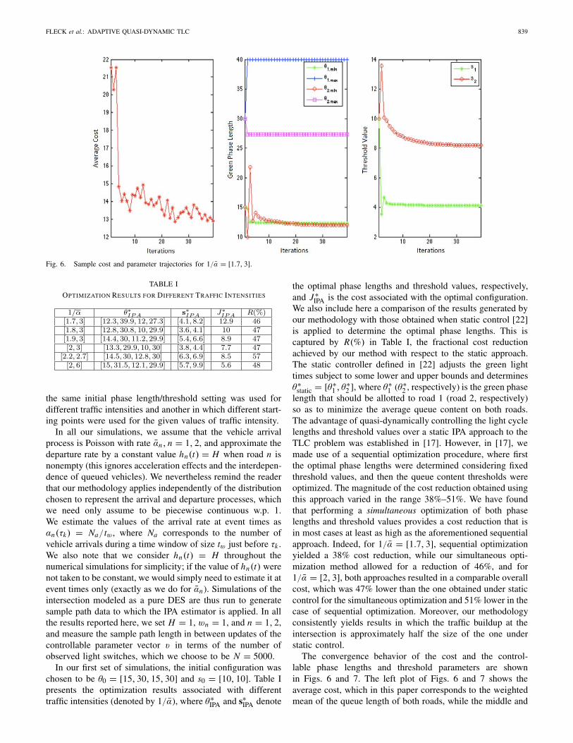
Fig. 8. Simulated traffic flow variation for 1/α = [2.2, 2.7].

right plots display the convergence behavior of the green phaselengths and threshold values, respectively. It is worthwhileto note that, in most of the analyzed scenarios, the valueof the average cost converges much more slowly than thevalues of the controllable parameters, but we remind thereader that the purpose of our work is precisely to identifycontrollable parameters whereby an effective quasi-dynamic

TLC may be imposed. As such, existing oscillations in theaverage cost value, albeit small once the green phase lengthsand threshold values have converged, point to the robustness ofour proposed approach. We also draw the reader’s attention tothe difference in the convergence time between the green phaselength parameters and threshold parameters. It can be observedin Figs. 6 and 7 that the real challenge in convergence lies


with the threshold values, which represent the quasi-dynamicparameters introduced by our methodology, while the greenphase lengths generally converge much faster to their optimalconfiguration.

In our second set of simulations, we analyze the con-vergence results in light of the existence of local minima,and three different traffic intensity settings are contemplated.Table II summarizes the results obtained when different initialconfigurations (θ0 and s0 values) are used. It comes as nosurprise that local minima exist throughout the 6-D cost sur-face of this system so that the optimal configuration to whichthe algorithm converges is dependent on the starting point.More interesting, however, is the fact that, for any given trafficintensity, we are able to consistently achieve a cost reductionof the order of 50% across different optimal configurations.

We also include an example of the simulated traffic flowvariation in Fig. 8, which presents the queue content onboth roads as a function of the simulation time. For easeof visualization, the entire sample path length in betweenupdates of the controllable parameters is not shown in Fig. 8.Nevertheless, it is possible to note that the queue lengths onboth roads become increasingly bounded as the simulationprogresses. This indicates that, as the algorithm converges tooptimal phase length and threshold settings, the number ofvehicles on each road tends to oscillate within tighter bounds,whose values are directly related to the optimal thresholdvalues determined for each road.

V. CONCLUSION

We have modeled a single traffic light intersection as anSFM and formulated the corresponding TLC problem withina quasi-dynamic control setting to which IPA techniqueswere applied in order to derive gradient estimates of a costmetric with respect to controllable phase lengths and queuecontent threshold values. By subsequently incorporating theseestimators into a gradient-based optimization algorithm andsimultaneously determining the optimal phase length/thresholdconfiguration, we were able to reduce traffic buildup byapproximately half (with respect to the traffic buildup resultingfrom a system operating under static control). Such resultswere consistently observed across a range of different traf-fic intensity settings and provide strong evidence of theadvantages of applying an IPA-based quasi-dynamic controlframework to the TLC problem. Our ongoing research isnow focused on applying IPA to an intersection with morecomplicated traffic flows, e.g., allowing for left and rightturns. The presence of more competing flows implies theneed for also controlling the light phase sequence, which ourmethodology can handle by defining additional parameters(e.g., redefining the control vector θ by adding constraints thatdictate the number of mutually exclusive flows). We are alsoaiming to incorporate acceleration/deceleration due to lightswitches into the model, as well as extending our methodologyto a network of multiple intersections. Assuming that trafficlights can communicate with each other, it is also possibleto endow a downstream light with the ability to predict animpending flow of vehicles and adjust its light cycle within

the proposed quasi-dynamic framework, i.e., by adjusting itsthreshold parameters accordingly. Finally, it is worth acknowl-edging the emergence of a virtual traffic light setting [43],in which case IPA techniques are equally applicable to theswitching control of a virtual rather than actual traffic light.

REFERENCES

[1] B. Abdulhai, R. Pringle, and G. J. Karakoulas, “Reinforcement learningfor true adaptive traffic signal control,” J. Transp. Eng., vol. 129, no. 3,pp. 278–285, 2003.

[2] I. Alvarez and A. Poznyak, “Game theory applied to urban trafficcontrol problem,” in Proc. Int. Conf. Control, Autom. Syst., Oct. 2010,pp. 2164–2169.

[3] A. L. C. Bazzan, “Opportunities for multiagent systems and multiagentreinforcement learning in traffic control,” Auto. Agents Multi-Agent Syst.,vol. 18, no. 3, pp. 342–375, Jun. 2009.

[4] C. G. Cassandras, “Event-driven control and optimization in hybridsystems,” in Event-Based Control and Signal Processing. Boca Raton,FL, USA: CRC Press, 2015, To appear.

[5] C. G. Cassandras and S. Lafortune, Introduction to Discrete EventSystems. New York, NY, USA: Springer-Verlag, 2008.

[6] C. G. Cassandras, Y. Wardi, B. Melamed, G. Sun, and C. G. Panayiotou,“Perturbation analysis for online control and optimization of sto-chastic fluid models,” IEEE Trans. Autom. Control, vol. 47, no. 8,pp. 1234–1248, Aug. 2002.

[7] C. G. Cassandras, Y. Wardi, C. G. Panayiotou, and C. Yao, “Perturbationanalysis and optimization of stochastic hybrid systems,” Eur. J. Control,vol. 16, no. 6, pp. 642–661, 2010.

[8] W. Choi, H. Yoon, K. Kim, I. Chung, and S. Lee, “A traffic lightcontrolling FLC considering the traffic congestion,” in Proc. AFSS Int.Conf. Fuzzy Syst., 2002, pp. 69–75.

[9] U.S. Department of Transportation Federal HighwayAdministration. (2013). Traffic Signal Timing Manual. [Online].Available: http://ops.fhwa.dot.gov/publications/fhwahop08024.htm

[10] C. Dong, “Area traffic signal timing optimization based on chaoticand genetic algorithm approach,” Comput. Eng. Appl., vol. 40, no. 29,pp. 32–34, 2004.

[11] C. Dong, “Chaos-particle swarm optimization algorithm and its applica-tion to urban traffic control,” Int. J. Comput. Sci. Netw. Secur., vol. 61,no. 1, pp. 97–101, 2006.

[12] C. Dong, Z. Liu, and Z. Qiu, “Urban traffic signal timing optimizationbased on multi-layer chaos neural networks involving feedback,” in Proc.1st Int. Conf. Natural Comput., 2005, pp. 340–344.

[13] F. Dressler, H. Hartenstein, O. Altintas, and O. Tonguz, “Inter-vehiclecommunication: Quo vadis,” IEEE Commun. Mag., vol. 52, no. 6,pp. 170–177, Jun. 2014.

[14] Y. Dujardin, F. Boillot, D. Vanderpooten, and P. Vinant, “Multiobjectiveand multimodal adaptive traffic light control on single junctions,”in Proc. IEEE Int. Conf. Intell. Transp. Syst., Oct. 2011,pp. 1361–1368.

[15] N. V. Findle, S. Surender, and S. Catrava, “On-line decisionsabout permitted/protected left-hand turns in distributed traffic signalcontrol,” Eng. Appl. Artif. Intell., vol. 10, no. 3, pp. 315–320,Jun. 1997.

[16] N. V. Findler and J. Stapp, “Distributed approach to optimized controlof street traffic signals,” J. Transp. Eng., vol. 118, no. 1, pp. 99–110,Jan. 1992.

[17] J. L. Fleck and C. G. Cassandras, “Infinitesimal perturbation analysis forquasi-dynamic traffic light controllers,” in Proc. Int. Workshop DiscreteEvent Syst., 2014, pp. 235–240.

[18] M. C. Fu and W. C. Howell, “Application of perturbation analysisto traffic light signal timing,” in Proc. IEEE Conf. Decision Control,Dec. 2003, pp. 4837–4840.

[19] N. J. Garber and L. A. Hoel, Traffic and Highway Engineering, 4th ed.Boston, MA, USA: Cengage Learning, 2009.

[20] N. H. Gartner, “OPAC: A demand responsive strategy for traffic signalcontrol,” J. Transp. Res. Board, vol. 1, no. 906, pp. 75–81, 1983.

[21] Y. Geng and C. G. Cassandras, “Multi-intersection traffic light con-trol using infinitesimal perturbation analysis,” in Proc. Int. WorkshopDiscrete Event Syst., 2012, pp. 104–109.

[22] Y. Geng and C. G. Cassandras, “Traffic light control using infinitesimalperturbation analysis,” in Proc. IEEE Conf. Decision Control, Dec. 2012,pp. 7001–7006.


[23] Y. Geng and C. G. Cassandras. (2013). “Quasi-dynamic traf-fic light control for a single intersection.” [Online]. Available:http://arxiv.org/abs/1308.0864

[24] Y. Geng and C. G. Cassandras, “Multi-intersection traffic light controlwith blocking,” J. Discrete Event Dyn. Syst., vol. 25, nos. 1–2, pp. 7–30,Jun. 2015.

[25] L. Head, F. Ciarallo, and D. L. Kaduwela, “A perturbation analy-sis approach to traffic signal optimization,” in INFORMS Nat.Meeting, 1996.

[26] J. J. Henry and J. L. Farges, “PRODYN,” in Proc. IFAC/IFIP/IFORSSymp., Paris, France, Sep. 1989, pp. 253–255.

[27] J. J. Henry, J. L. Farges, and J. L. Gallego, “Neuro-fuzzy techniquesfor traffic control,” Control Eng. Pract., vol. 6, no. 6, pp. 755–761,Jun. 1998.

[28] W. C. Howell and M. C. Fu. (2006). Simulation Optimization of TrafficLight Signal Timings via Perturbation Analysis. [Online]. Available:http://citeseerx.ist.psu.edu/viewdoc/summary?doi=10.1.1.362.3837

[29] P. B. Hunt, D. I. Robertson, R. D. Bretherton, and M. C. Royle, “TheSCOOT on-line traffic signal optimization technique,” in Proc. Int. Conf.Road Traffic Signaling, Mar./Apr. 1982, pp. 59–62.

[30] J. D. C. Little, M. D. Kelson, and N. H. Gartner, “MAXBAND: Aprogram for setting signals on arteries and triangular networks,” inProc. Transp. Res. Rec. 795, Traffic Flow Theory Characteristics, 1981,pp. 40–46.

[31] Z. Liu, “A survey of intelligence methods in urban traffic signal control,”Int. J. Comput. Sci. Netw. Secur., vol. 7, no. 7, pp. 105–112, 2007.

[32] P. R. Lowrie, “The Sydney coordinated adaptive traffic system—Principles, methodology, algorithms,” in Proc. IEE Conf. Road TrafficSignaling, 1982, pp. 67–70.

[33] C. G. Panayiotou, W. C. Howell, and M. C. Fu, “Online traffic lightcontrol through gradient estimation using stochastic fluid models,” inProc. IFAC Triennial World Congr., Jul. 2005.

[34] C. P. Pappis and E. H. Mamdani, “A fuzzy logic controller for a trafficjunction,” IEEE Trans. Syst., Man, Cybern., vol. 7, no. 10, pp. 707–717,Oct. 1977.

[35] I. Porche, M. Sampath, R. Sengupta, Y.-L. Chen, and S. Lafor-tune, “A decentralized scheme for real-time optimization of traf-fic signals,” in Proc. IEEE Int. Conf. Control Appl., Sep. 1996,pp. 582–589.

[36] L. A. Prashanth and S. Bhatnagar, “Reinforcement learning with functionapproximation for traffic signal control,” IEEE Trans. Intell. Transp.Syst., vol. 12, no. 2, pp. 412–421, Jun. 2011.

[37] D. I. Robertson, “TRANSYT method for area traffic control,” TrafficEng. Control, vol. 11, no. 6, pp. 276–281, 1969.

[38] B. De Schutter, “Optimal traffic light control for a single intersection,”in Proc. Amer. Control Conf., Jun. 1999, pp. 2195–2199.

[39] S. Sen and K. L. Head, “Controlled optimization of phases at anintersection,” Transp. Sci., vol. 31, no. 1, pp. 5–17, 1997.

[40] S. G. Shelby, D. M. Bullock, D. Gettman, R. S. Ghaman, Z. A. Sabra,and N. Soyke, “An overview and performance evaluation of ACS lite—A low cost adaptive signal control system,” in Proc. 87th Annu. MeetingTransp. Res. Board, Jan. 2008.

[41] J. C. Spall and D. C. Chin, “Traffic-responsive signal timing for system-wide traffic control,” Transp. Res. C, Emerg. Technol., vol. 5, nos. 3–4,pp. 153–163, Aug./Oct. 1997.

[42] T. Tettamanti, T. Luspay, B. Kulcsar, T. Peni, and I. Varga, “Robustcontrol for urban road traffic networks,” IEEE Trans. Intell. Transp.Syst., vol. 15, no. 1, pp. 385–398, Feb. 2014.

[43] O. Tonguz, W. Viriyasitavat, and J. Roldan, “Implementing virtualtraffic lights with partial penetration: a game-theoretic approach,” IEEECommun. Mag., vol. 52, no. 12, pp. 173–182, 2014.

[44] S. V. Ukkusuri, G. Ramadurai, and G. Patil, “A robust transportationsignal control problem accounting for traffic dynamics,” Comput. Oper.Res., vol. 37, no. 5, pp. 869–879, May 2010.

[45] Y. Wardi, R. Adams, and B. Melamed, “A unified approach toinfinitesimal perturbation analysis in stochastic flow models: Thesingle-stage case,” IEEE Trans. Autom. Control, vol. 55, no. 1,pp. 89–103, Jan. 2010.

[46] W. Wen, “A dynamic and automatic traffic light control expert systemfor solving the road congestion problem,” Expert Syst. Appl., vol. 34,no. 4, pp. 2370–2381, 2008.

[47] Y. Wen and T. Wu, “Reduced-order rolling horizon optimization of trafficcontrol based on ant algorithm,” J. Zhejiang Univ. (Eng. Sci.), vol. 39,no. 6, pp. 835–839, 2005.

[48] W.-M. Wey, “Model formulation and solution algorithm of traffic signalcontrol in an urban network,” Comput., Environ. Urban Syst., vol. 24,no. 4, pp. 355–378, Jul. 2000.

[49] M. Wiering, J. van Veenen, J. Vreeken, and A. Koopman, “Intelligenttraffic light control,” Inst. Inf. Comput. Sci., Utrecht Univ., Utrecht,The Netherlands, Tech. Rep. UU-CS-2004-029, 2004.

[50] C. Yao and C. G. Cassandras, “Perturbation analysis of stochastic hybridsystems and applications to resource contention games,” Frontiers Elect.Electron. Eng. China, vol. 6, no. 3, pp. 453–467, Sep. 2011.

[51] Y. Yin, “Robust optimal traffic signal timing,” Transp. Res. B, Methodol.,vol. 42, no. 10, pp. 911–924, Dec. 2008.

[52] X.-H. Yu and W. W. Recker, “Stochastic adaptive control model fortraffic signal systems,” Transp. Res. C, Emerg. Technol., vol. 14, no. 4,pp. 263–282, Aug. 2006.

[53] X. Zhao and Y. Chen, “Traffic light control method for a singleintersection based on hybrid systems,” in Proc. IEEE Int. Conf. Intell.Transp. Syst., Oct. 2003, pp. 1105–1109.

Julia L. Fleck received the B.Eng. degree inchemical engineering from the Federal Universityof Rio de Janeiro, Rio de Janeiro, Brazil, in 2006,and the M.S. degree in mechanical engineeringfrom the Catholic University of Rio de Janeiro,Rio de Janeiro, in 2008. She is currently pursuingthe Ph.D. degree with the Division of Systems Engi-neering, Boston University, Brookline, MA, USA.

She was a Researcher with Tecgraf/PUC-Rio,Rio de Janeiro, from 2008 to 2011, where she wasinvolved in the development of artificial intelligence

algorithms for enhanced oil recovery. Her current research interests includestochastic hybrid systems, optimal control, and stochastic optimization.

Christos G. Cassandras (F’96) received theB.S. degree from Yale University, New Haven, CT,USA, in 1977, the M.S.E.E. degree from StanfordUniversity, Stanford, CA, USA, in 1978, and theM.S. and Ph.D. degrees from Harvard University,Cambridge, MA, USA, in 1979 and 1982,respectively.

He was with ITP Boston, Inc., Cambridge,from 1982 to 1984, where he was involved inthe design of automated manufacturing systems.From 1984 to 1996, he was a Faculty Member

with the Department of Electrical and Computer Engineering, University ofMassachusetts Amherst, Amherst, MA, USA. He is currently a DistinguishedProfessor of Engineering with Boston University, Brookline, MA, USA,the Head of the Division of Systems Engineering, and a Professor ofElectrical and Computer Engineering. He specializes in the areas of discreteevent and hybrid systems, cooperative control, stochastic optimization, andcomputer simulation, with applications to computer and sensor networks,manufacturing systems, and transportation systems. He has authoredover 350 refereed papers in these areas, and five books.

Dr. Cassandras is a member of Phi Beta Kappa and Tau Beta Pi. He isalso a fellow of the International Federation of Automatic Control (IFAC).He was a recipient of several awards, including the 2011 IEEE Control Sys-tems Technology Award, the 2006 Distinguished Member Award of the IEEEControl Systems Society, the 1999 Harold Chestnut Prize (IFAC Best ControlEngineering Textbook), a 2011 prize and a 2014 prize for the IBM/IEEESmarter Planet Challenge competition, the 2014 Engineering DistinguishedScholar Award at Boston University, several honorary professorships, a 1991Lilly Fellowship, and a 2012 Kern Fellowship. He was the Editor-in-Chief ofthe IEEE TRANSACTIONS ON AUTOMATIC CONTROL from 1998 to 2009.He serves on several editorial boards and has been a Guest Editor for variousjournals. He was the President of the IEEE Control Systems Society in 2012.

Yanfeng Geng (S’11) received the B.S. degreefrom the University of Science and Technology ofChina, Hefei, China, in 2005, and the Ph.D. degreefrom the Division of Systems Engineering, BostonUniversity, Brookline, MA, USA, in 2013.

He is currently with Amazon in Boston, MA, USA.His current research interests include intelligenttransportation system, optimal control, andstochastic optimization.

Documents

830 IEEE TRANSACTIONS ON CONTROL SYSTEMS …people.bu.edu/cgc/Published/TCSTprint_03_16.pdf830 IEEE TRANSACTIONS ON CONTROL SYSTEMS TECHNOLOGY, VOL. 24, NO. 3, MAY 2016 Adaptive Quasi-Dynamic