8.5 Lagrangian and Hamiltonian Formalism in Field Theorieszwirner/DT-ch8parte.pdf · 2014-01-09 · 8.5 Lagrangian and Hamiltonian Formalism in Field Theories 233 on the values of

232 8 Lagrangian and Hamiltonian Formalism

8.5 Lagrangian and Hamiltonian Formalism in Field Theories

Our discussion has been confined so far to mechanical systems with a finite numberof degrees of freedom, q1(t), . . . , qn(t).

This has been propaedeutic to our principal interest, namely the description ofcontinuous systems, hereafter called fields. A well known example of field is the elec-tromagnetic field whose description is given in terms of the four-potential Aµ(x, t);that means that, at any instant t , its configuration is defined by assigning, for eachcomponent µ, the value of Aµ(x, t) at each point x in space.

In this case we have a continuous infinity of canonical coordinates qi (t) =Aµ(x, t), labeled by the three coordinates x for the space-point and the indexµ.14 Other examples of fields are the continuous matter fields like fluids, elasticmedia, etc.

Quite generally we may view a continuous system as the limit of a mechanicalsystem described by a finite number of degrees of freedom qi (discrete system), byletting i become the continuous index x. As a consequence every sum !i over thediscrete label i will be replaced by an integration on d3x over a spatial domain V ,usually the whole three-dimensional space15:

!

i

!"

V

d3x.

In the following we shall consider fields "#(x, t) carrying an (internal) index#, where # labels the components of a “vector " " ("#)” on which a repre-sentation of a group G acts. If # has just one value, it will be omitted and we speakof a scalar field. In relativistic field theories, the group G will often be the Lorentzgroup O(1, 3) so that the index will label a basis of the carrier of a representationof the Lorentz group.16 For example, in the case of the electromagnetic field, therole of # is played by the index µ pertaining to the four-dimensional fundamentalrepresentation of SO(1, 3).

8.5.1 Functional Derivative

When we think of fields as a continuous limit of discrete systems, the correspondingLagrangian obtained in the limit, L("#, $t"

#, t), will depend, at a certain instant t,

14 More precisely, since x " (x1, x2, x3), we have a triple infinity of Lagrangian coordinates qi (t)for each value of the index µ = 0, 1, 2, 3. The three components of x and the index µ play therole of the index iof the discrete case.15 Actually in our treatment of a discrete number of degrees of freedom, we have often omitted thesymbol ! when there are repeated indices.16 Somewhat improperly, by the word representation people often refer to the carrier space Vp ofa representation. We shall also do this to simplify the exposition and thus talk about a basis of arepresentation when referring to a basis of the corresponding carrier space.

8.5 Lagrangian and Hamiltonian Formalism in Field Theories 233

on the values of the fields "#(x, t) and $t"#(x, t) at every point in the domain V of

the three-dimensional space. We say in this case that the Lagrangian is a functionalof "#(x, t) and $t"

#(x, t), viewed as functions of x. It will be convenient in thefollowing to denote by "#(t) the function "#(x, t) of the point x in space at a giventime t , and by "#(t) its time derivative "#(x, t) " $t"

#(x, t). We shall presentlyexplore some property of functionals. Let us consider a functional F["], and performan independent variation of "(x), at each space point x. The corresponding variationof F["] will be:

%F["] " F[" + %"] # F["] ="

%F["]%"(x)

%"(x)d3x, (8.103)

where by definition, %F["]%"(x) is the functional derivative of F["] with respect to " at

the point x. Here we have suppressed the possible dependence on time of " and ofthe functional F either explicitly or through ": " = "(x, t), F = F["(t), t].

From its definition it is easy to verify that the functional derivation enjoys the sameproperties as the ordinary one, namely it is a linear operator, vanishes on constantsand satisfies the Leibnitz rule.

When the functional depends on more than a single function, its definition canbe extended correspondingly, as for ordinary derivatives. Of particular relevance forus is the additional dependence of F on the time derivative $t"(x, t) of "(x, t).Moreover we may consider a set of fields "# labeled by the index # pertainingto a given representation of a group G. This is the case of the Lagrangian F =L("#(t), "#(t), t), where we recall once again that, in writing "(t), "(t) among thearguments of the Lagrangian, we mean that L depends on the values "(x, t), "(x, t)of these fields in every point x in space at a given time t. Applying the definition(8.103) to the two functions "#(t) and "#(t) we have:

%L("#(t), "#(t), t) ="

d3x#

%L%"#(x, t)

%"#(x, t) + %L%"#(x, t)

%"#(x, t)$

. (8.104)

Note that the Lagrangian depends on t either through "# and "# or explicitly. TheLagrangian, as a functional with respect to the space-dependence of the fields, can bethought of as the continuous limit of a function of infinitely many discrete variables:

L("i (t), "i (t), t)i!x#! L("(t), "(t), t).

Here and in the following we shall often omit the index # if not essential to ourconsiderations. Correspondingly, we can show that the functional derivative definedabove can be thought of as a suitable continuous limit of the ordinary derivative withrespect to a discrete set of degrees of freedom qi , described by a Lagrangian L(qi , qi ).

Let us indeed regard the values of "(x, t) at each point x as independent canonicalcoordinates. To deal with a continuous infinity of canonical coordinates, we dividethe 3-space into tiny cells of volume %V i . Let "i (t) be the mean value of "(x, t)inside the i th cell and L(t) = L("i (t), "i (t), t) be the Lagrangian, depending on


the values "i (t), "i (t) of the field and its dime derivative in every cell. The variation%L("i , "i ) can be written as

%L("i (t), "i (t), t) =!

i

%$L$"i %"i + $L

$"i %"i

&

=!

i

1%V i

%$L$"i %"i + $L

$"i %"

&%V i , (8.105)

If we compare this expression with (8.104), in the continuum limit one can make thefollowing identification:

%L%"(x, t)

" lim%V i !0

1%V i

$L$"i ,

%L%"(x, t)

" lim%V i !0

1%V i

$L$("i )

,

(8.106)

where x is in the i th cell. In the limit %Vi ! 0 we can set %Vi " d3x. Thus thefunctional derivative %L(t)/%"(x, t) is essentially proportional to the derivative ofL with respect to the value of " at the point x. Since in the discretized notation theaction principle leads to the equations of motion:

$L(t)$"i

# $t$L(t)$"i (t)

= 0 (8.107)

in the continuum limit the Euler–Lagrange equations become:

%L%"#(x, t)

# $t%L

%"#(x, t)= 0. (8.108)

where we have reintroduced the index # of the general case.In the discretized notation we shall assume the Lagrangian L , which depends

on the values of the fields and their time derivatives in every cell, to be the sum ofquantities Li defined in each cell: Li depends on the values of the field "#

i (t), itsgradient !"#

i and its time derivative "#i (t) in the i th cell only:

L("#i (t), "#

i (t), t) =!

i

Li ("#i (t),!"#

i (t), "#i (t), t). (8.109)

Multiplying and dividing the right hand side by %Vi and taking the continuum limit%Vi ! d3x, the above equality becomes

L("#(t), "#(t), t) ="

V

d3xL("#(x),!"#(x), "#(x); x, t), (8.110)

where x " (xµ) = (ct, x) and we have defined the Lagrangian density L as


L("#(x),!"#(x), "#(x); x, t) " lim%Vi !0

1%Vi

Li ("#i (t),!"#

i (t), "#i (t), t).

Just as Li depends, at a time t , on the dynamic variables referred to the i-th cell only,L is a local quantity in Minkowski space in that it depends on both x and t. We notethe appearance in L(x) of the space derivatives !"#(x, t). This follows from thefact that in order to have an action which is a scalar under Lorentz transformations,L itself must be a Lorentz scalar. Since Lorentz transformations will in general shuffletime and space derivatives, L should then depend on all of them. The action, in termsof the Lagrangian density, will read:

S["#; t1, t2] =t2"

t1

L(t)dt ="

dtd3xL(x) = 1c

"

D4

d4xL(x), (8.111)

where D4 is a space–time domain: An event x " (xµ) in D4 occurs at a timet between t1 and t2 and at a point x in the volume V . In formulas we will writeD4 " [t1, t2] $ V % M4. Since S does not depend only on the time interval [t1, t2]but also on the volume V in which the values of the fields and their derivativesare considered, we will write S " S["#; D4]. The boundary of D4, to be denotedby $ D4, consists of all the events occurring either at t = t1 or at t = t2, and ofevents occurring at a generic t & [t1, t2] in a point x belonging to the surface SVwhich encloses the volume V : x & SV " $V . The measure of integration d4x "dx0dx1dx2dx3 = cdtd3x is invariant under Lorentz transformations ! = (&

µ' ),

since the absolute value |det(!)| of the determinant of the corresponding Jacobianmatrix !, is equal to one:

xµ #! x 'µ = &µ' x' ( d4x #! d4x ' = |det(!)|d4x = d4x . (8.112)

It follows that in order to have a scalar Lagrangian density L must have the samedependence on !"#(x, t) as on "#(x, t), that is it must actually depend on thefour-vector $µ"#(x, t). Moreover, being a scalar, it must depend on the fields andtheir derivatives $µ"#(x, t) only through invariants constructed out of them. Forthe same reason it cannot depend on t only, but, in general, on all the space–timecoordinates xµ.

Let us now consider arbitrary infinitesimal variations of the field "#(x) whichvanish at the boundary $ D4 of D4 : %"#(x) " 0 if x & $ D4. The correspondingvariation of L can be computed by using (8.110):

%L ="

d3x#

$L(x, t)$"#(x, t)

%"#(x, t) + $L(x, t)$$i "#(x, t)

%$i "#(x, t)

+ $L(x, t)$("#(x, t))

%"#(x, t)$

="

d3x'#

$L(x, t)$"#(x, t)

# $i$L(x, t)

$$i "#(x, t)

$%"#(x, t) # $L(x, t)

$"#(x, t)%"#(x, t)

(, (8.113)


where we have written ! " ($i )i=1,2,3, used the property that %$i"# = $i%"

# andintegrated the second term within the integral by parts, dropping the surface term,being %"#(x) = 0 for x & SV " $V .

Taking into account that the quantity inside the curly brackets defines the func-tional derivative of L , by comparison with (8.108) we find:

%L%"#(x)

=#

$L(x)

$"#(x)# $i

$L(x)

$$i"#(x)

$,

%L%"#(x)

= $L(x)

$"#(x). (8.114)

It is important to note that, using the Lagrangian density instead of the Lagrangian, thederivatives of L(x, t) with respect to the fields in (x, t) are now ordinary derivatives,since they are computed at a particular point x. Using the equalities (8.114) theEuler–Lagrange equations (8.108) take the following form:

$t$L

$($t"#)= $L

$"## $i

$L$($i"#)

, (8.115)

or, using a Lorentz covariant notation:

$L$"#

# $µ

%$L

$($µ"#)

&= 0. (8.116)

8.5.2 The Hamilton Principle of Stationary Action

In the previous paragraph the equations of motion for fields have been derived usingthe definition of functional derivative and performing the continuous limit of theEuler–Lagrange equations for a discrete system.

Actually (8.116), can also be derived directly from the Hamilton principle of sta-tionary action, considering the action S as a functional of the fields "#and dependingon the space-time domain D4 on which they are defined:

S)"#; D4

*= 1

c

"

D4

d4xL("#, $µ"#, xµ). (8.117)

Here d4x " dx0d3x = cdtd3x is the volume element in the Minkowski space M4,and the integration domain D4 was defined as [t1, t2] $ V % M4.

We can now generalize the Hamilton principle of stationary action to systemsdescribed by fields, namely systems exhibiting a continuous infinity of degrees offreedom. It states that:

The time evolution of the field configuration describing the system is obtained byextremizing the action with respect to arbitrary variations of the fields %"# whichvanish at the boundary $ D4 of the space–time domain D4.


Precisely, we require the action S to be stationary with respect to %"# , that is tosatisfy

%S = 0,

under arbitrary variations of "# at each point x and at each instant t:

"#(x) ! "#(x) + %"#(x),

provided:

%"#(x) = 0 )xµ & $ D4. (8.118)

Let us apply this principle to the action (8.117). We have:

%S = 1c

"

D4

d4x%

$L$"#

%"# + $L$($µ"#)

%($µ"#)

&. (8.119)

Now use the property %($µ"#) = $µ(%"#), and integrate by parts the second termin the integral:"

D4

d4x$L

$($µ"#)$µ%"# =

"

D4

d4x$µ

%$L

$($µ"#)%"#

&

#"

D4

d4x$µ

%$L

$($µ"#)

&%"# =

"

$ D4

d4(µ

%$L

$($µ"#)

&%"#

#"

D4

d4x$µ

%$L

$($µ"#)

&%"# = #

"

D4

d4x$µ

%$L

$($µ"#)

&%"#,

where we have applied the four-dimensional version of the divergence theorem byexpressing the integral of a four-divergence over D4 as an integral (boundary integral)of the four-vector $L

$($µ"#)%"# over the three-dimensional domain $ D4 which encloses

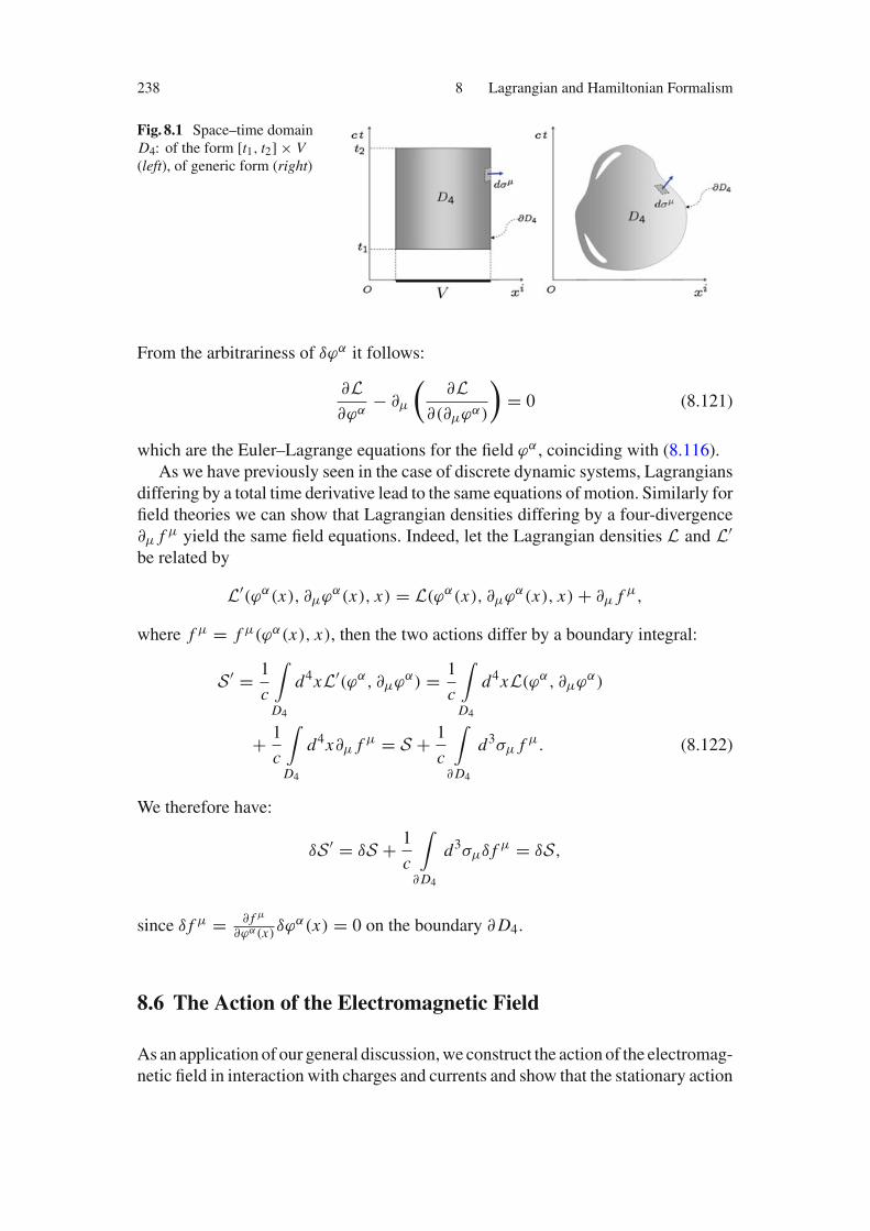
D4. We have used the notation d3(µ " d3(nµ, d3( being an element of $ D4 towhich the unit norm vector nµ is normal, see Fig. 8.1. As for the last equality wehave used (8.118) which implies the vanishing of the boundary integral.17 Thus thepartial integration finally gives:

%S = 1c

"

D4

d4x#

$L$"#

# $µ

%$L

$($µ"#)

&$%"#. (8.120)

17 This is true if the boundary $ D4 does not extend to spatial infinity; when the integration domainD4 fills the whole space, we must require that the fields and their derivatives fall off sufficientlyfast at infinity, or we may also use periodic boundary conditions. In any case the integration on aninfinite domain can always be taken initially on a finite domain, and, after removing the boundaryterm, the integration domain can be extended to infinity.


Fig. 8.1 Space–time domainD4: of the form [t1, t2] $ V(left), of generic form (right)

From the arbitrariness of %"# it follows:

$L$"#

# $µ

%$L

$($µ"#)

&= 0 (8.121)

which are the Euler–Lagrange equations for the field "# , coinciding with (8.116).As we have previously seen in the case of discrete dynamic systems, Lagrangians

differing by a total time derivative lead to the same equations of motion. Similarly forfield theories we can show that Lagrangian densities differing by a four-divergence$µ f µ yield the same field equations. Indeed, let the Lagrangian densities L and L'

be related by

L'("#(x), $µ"#(x), x) = L("#(x), $µ"#(x), x) + $µ f µ,

where f µ = f µ("#(x), x), then the two actions differ by a boundary integral:

S ' = 1c

"

D4

d4xL'("#, $µ"#) = 1c

"

D4

d4xL("#, $µ"#)

+ 1c

"

D4

d4x$µ f µ = S + 1c

"

$ D4

d3(µ f µ. (8.122)

We therefore have:

%S ' = %S + 1c

"

$ D4

d3(µ% f µ = %S,

since % f µ = $ f µ

$"#(x)%"#(x) = 0 on the boundary $ D4.

8.6 The Action of the Electromagnetic Field

As an application of our general discussion, we construct the action of the electromag-netic field in interaction with charges and currents and show that the stationary action

8.6 The Action of the Electromagnetic Field 239

principle gives the covariant form of the Maxwell equations discussed in Chap. 5.To this end we shall be guided by the symmetry principle. As it will be shown indetail in Sect. 8.7, the invariance of the equations of motion under space-time (i.e.Poincaré) transformations or under general field transformations is guaranteed if theLagrangian density, as a function of the fields, their derivatives and the space-timecoordinates, is invariant in form, up to a total divergence, see Eq. (8.150). As far asspace-time translations are concerned, this is the case if L does not explicitly dependon xµ. Covariance with respect to Lorentz transformations further requires L to beinvariant as a function of the fields and their derivatives, namely to be a Lorentzscalar as a function of space-time.

The construction of the action for the electromagnetic field is relatively simpleonce we observe that:

• For the field Aµ(x) describing the electromagnetic field the generic index # coin-cides with the covariant index µ = 0, 1, 2, 3 of the fundamental representation ofthe Lorentz group;

• The equations of motion (the Maxwell equations) are invariant under the gaugetransformations:

Aµ ! Aµ + $µ".

This is guaranteed if the Lagrangian density is invariant under the same transfor-mations, since the action would then be invariant. In the absence of charges andcurrents, the action should be constructed out of the gauge invariant quantity Fµ';

• The Lagrangian density must be a scalar under Lorentz transformations;• In order for the equations of motion to be second-order differential equations L

must at most be quadratic in the derivatives of Aµ(x), that is quadratic in Fµ' .

To construct Lorentz scalars which are quadratic in Fµ' we may use the invarianttensors )µ', *µ'+( of the Lorentz group SO(1, 3).18 It can be easily seen that the mostgeneral Lagrangian density satisfying the previous requirements has the followingform:

L(Aµ, $µ A') = aFµ' Fµ' + b*µ'+( Fµ' F+( , (8.123)

where Fµ' = )µ+)'( F+( and a and b are numerical constants. On the other hand,the second term of (8.123) is the four-dimensional divergence of a four-vector sothat it does not contribute to the equations of motion. Indeed:

*µ'+( Fµ' F+( = 2*µ'+( $µ A' F+(

= $µ+2*µ'+( A' F+(

,# 2*µ'+( A'$µF+(

= $µ+2*µ'+( A' F+(

,# 2*µ'+( A'$ [µF+( ]

= $µ f µ,

18 Recall that the latter tensor *µ'+( is not invariant under Lorentz transformations which are inO(1, 3) but not in SO(1, 3), namely which have determinant #1. Examples of these are the paritytransformation !P , or time reversal !T .


where we have set: f µ = 2*µ'+( A' F+( and use has been made of the identity:$ [µF+( ] = 0.

Therefore the Lagrangian density reduces, up to a four-dimensional divergenceto the single term:

Lem = aFµ' Fµ' .

The value of the constant a is fixed in such a way that the Lagrangian contains thepositive definite (density of) “kinetic term” 1/(2c2) $t Ai$t Ai with a conventionalfactor 1/2 which is remnant of the one appearing in the definition (8.25) of thekinetic energy.19 Expanding Fµ' Fµ' = ($µ A' # $' Aµ)($µ A' # $' Aµ) one easilyfinds a = # 1

4 .

In the presence of charges and currents, the interaction with the source Jµ(x)

requires adding an interaction term Lint to the pure electromagnetic Lagrangian.The simplest interaction is described by the Lorentz scalar term:

Lint = bAµ Jµ. (8.124)

This term seems, however, to violate the gauge invariance of the totalLagrangian, since a gauge transformation on Aµ implies a correspondent changeon the Lagrangian density:

%Aµ = $µ" ( %(gauge)Lint = ($µ")Jµ.

On the other hand by a partial integration %Lint can be transformed as follows:

%Lint = $µ(" Jµ) # "$µ Jµ.

The first term is a total four-divergence, not contributing to the equations of motionand thus can be neglected; the second term is zero if and only if $µ Jµ = 0, that is ifthe continuity equation expressing the conservation of the electric charge holds. Wehave thus found the following important result: Requiring gauge invariance of theaction of the electromagnetic field interacting with a current, implies the conservationof the electric charge.

In conclusion, the action describing the electromagnetic field coupled to chargesand currents is given by

S = 1c

"

M4

d4x%

#14

Fµ' Fµ' + bAµ Jµ

&, (8.125)

where the (four)-current Jµ(x) has the following general form (see Chap. 5)20:

19 Note that the kinetic term for A0 is absent because of the antisymmetry of Fµ' .20 Note that we are describing the interaction of the electromagnetic field, possessing infinite degreesof freedom, with a system of n charged particles, having 3n degrees of freedom represented by then coordinate vectors x(k)(t), (k = i, . . . , n). The Dirac delta function formally converts the 3ndegrees of freedom of x(k)(t) into the infinite degrees of freedom associated to x.


Jµ(x) = 1c

!

k

ekdxµ

k

dt%3(x # xk(t)). (8.126)

We may now apply the principle of stationary action to compute the equationsof motion. Recalling the form (8.121) of the Euler–Lagrange equations for fields,we have:

$L$ Aµ

# $+

%$L

$($+ Aµ)

&= 0. (8.127)

The first term of (8.127) is easily computed and gives:

$L$ Aµ

= bJµ(x).

As far as the second term is concerned, only the pure electromagnetic part#1/4Fµ' Fµ' contributes to the variation, yielding:

$(F+( F+( )

$($µ A')= 2

#$ F+(

$($µ A')

$F+( = 4

$($+ A( )

$($µ A')F+( = %µ

+ %'( F+( = 4Fµ'(x).

Putting together these results, (8.127) becomes:

$µFµ'(x) + bJ '(x) = 0. (8.128)

Finally he constant b is fixed by requiring (8.128) to be identical to the Maxwellequation21:

$µFµ' = #J ',

and this fixes b to be 1. The final expression of the Lagrangian density therefore is:

L = Lem + Lint = #14

Fµ' Fµ' + Aµ Jµ. (8.129)

In order to give a complete description of the charged particles in interaction withthe electromagnetic field, we must add to L (8.129) the Lagrangian density Lpartassociated with system of particles.

Let us consider for the sake of simplicity the case of a single particle of charge eand mass m. The total action will have the following form22:

Stot = Sem + Sint + Spart , (8.130)

21 Note that this condition just fixes the charge normalization.22 The index k given to x(k) in the following formulae has a double function: On the one hand itindicates that the coordinate vector x(k)(t) is a dynamic variable, and not the labeling of the spacepoints, as is the case for x; On the other hand if we have more than one particle the followingformulae can be generalized by just summing over k.


where

Sem[$µ A'] = 1c

"d4x

%#1

4Fµ' Fµ'

&,

Spart [x(k)] = #mc2"

dt

-

1 #v2(k)

c2

. 12

,

Sint [Aµ(x), x(k), x(k)] = 1c

"d4x Aµ(x, t)Jµ(x, t)

= 1c

" /ec

Aµ(x(k), t)dxµ

(k)

dt

0

dt, (8.131)

where in deriving the expression of Sint23 we have used the explicit form of the

four-current given in (8.126).

Lint ="

d3xAµ(x, t)Jµ(x, t) = ec

Aµ(x(k), t)dxµ

(k)

dt

= eA0(x(k), t) + ec

Ai (x(k), t)vi . (8.132)

We recall that x are labels of the points in space, while x(k)(t) are the particle coor-dinates, that is dynamic variables, as stressed in the footnote.

We now observe that since Sem does not contain the variables xi(k), we may

compute the equation of motion of the charged particle by varying only L = L part +Lint:

L = L part + Lint = #mc2

1

1 #v2(k)

c2 + eA0(x(k), t) + ec

Ai (x(k), t)vi .

For the sake of simplicity in the following we neglect the index (k) of the particle.The first term of the Euler–Lagrange equations:

$ L$xi # d

dt$ L$vi = 0, (8.133)

reads:

$ L$xi = $Lint

$xi = e$ A0

$xi + ec

%$ A j

$xi

&v j . (8.134)

The second term contains the time derivative of the canonical momentum pi conju-gate to xi , namely:

23 Note that also Spart can be written as a four-dimensional integral:

Sint = #mc2

d4x%(3)(x # xk)3

1 # 1c2

+ dxdt

,24

.


pi = $ L$vi = $(L par + Lint )

$vi = m(v)vi + ec

Ai . (8.135)

We see that in the presence of the electromagnetic field the canonical conjugatemomentum is different from the momentum pi

(0) = m(v)vi of a free particle.24 Infact we have the following relation:

pi = pi(0) + e

cAi . (8.136)

Taking into account (8.133), (8.135) and (8.136), the equation of motion of thecharged particle becomes:

ddt

3pi(0) + e

cAi

4# e$i A0 # e

c$i A jv

j = 0. (8.137)

We now recall that A0 = #V, where V is the electrostatic potential. Moreover,since

d Ai

dt= $ Ai

$x j

dx j

dt+ c

$ Ai

$x0 ,

and Ei = Fi0 = $i A0 # $0 Ai , (8.137) becomes:

dpi(0)

dt= eEi # e

c

+$ j Ai # $i A j

,v j

= eEi # ec

Fjivj = eEi + e

c*i jkv

j Bk

= e%

Ei + 1c(v $ B)i

&.

Thus we have retrieved from the variational principle the well known equation ofmotion of a charged particle subject to electric and magnetic fields since the righthand side is by definition the Lorentz force.

8.6.1 The Hamiltonian for an Interacting Charge

As we have computed the Lagrangian Lint + L par for a charged particle, we pausefor a moment with our treatment of the Lagrangian formalism in field theories andcompute the Hamiltonian of a charge interacting with the electromagnetic field. Fromthe definition (8.64) we find25:

24 Here and in the following we use the subscript 0 to denote the usual free-particle momentumpi(0) = m(v)vi and the symbol pi for the momentum canonically conjugated to xi .

25 Recall that the vector A " (Ai ) is the spatial part of the four-vector Aµ " (A0, A), so that Aµ "(A0,#A). On the other hand p is the spatial component of pµ " (p0, p), so that pµ " (p0,#p).


H(p, x) = p · v # Lint # L par = p · v # eA0 # ec

A · v + m2c2

m(v),

where we have used the relation

#L part = mc2

1

1 # v2

c2 = m2c2

m(v).

It follows:

H(p, x) =3

p # ec

A4

· v + m2c2

m(v)+ eV (x). (8.138)

We now use (8.135) to express vi in terms of pi:

v =+p # e

c A,

m(v)= p(0)

m(v).

Taking into account the relativistic relations:

E2 = |p(0)|2c2 + m2c4; m(v) = E/c2, (8.139)

where E is the energy of the free particle, we can write:

H(p, x) = E2

m(v)c2 + eV = c

5m2c2 +

666p # ec

A6662+ eV (x). (8.140)

From the above equation we find:

(H + eA0)2 # c2

3!

i=1

3pi # e

cAi

42= m2c4. (8.141)

Next we use the property A0 = A0, Ai = #Ai to put (8.141) in relativistic invariantform:

3pµ + e

cAµ

4 3pµ + e

cAµ

4= m2c2. (8.142)

where we have set Hc = p0.

Note that (8.142) can be obtained from the relativistic relation pµ(0) p(0)µ = m2c2

of a free particle through the substitution:

pµ(0) ! pµ + e

cAµ. (8.143)

in agreement with (8.136). This substitution gives the correct coupling between theelectromagnetic field and the charged particle and is usually referred to as minimalcoupling.

8.7 Symmetry and the Noether Theorem 245

8.7 Symmetry and the Noether Theorem

In this section we explore the connection between symmetry transformation andconservation laws in field theory.

We consider a relativistic theory described by an action of the following form:

S)"#, D4

*= 1

c

"

D4

d4xL("#, $µ"#, xµ). (8.144)

where L("#, $µ"#, x) is the Lagrangian density.We consider a generic transformation of the coordinates xµ and of the fields "#:

xµ & D4 ! x 'µ = x 'µ(x) & D'4,

"# ! "'# = "'#("#, x),

$µ"# ! $µ'"'# = $ 'µ"'#("#, $µ"#, x).

(8.145)

where $ 'µ = $

$x 'µ . A transformation on space–time coordinates will in general deforma domain D4, which we had originally taken to be a direct product of a time intervaland a space volume V , into a region D'

4 with a different shape.As already discussed in the case of a discrete set of degrees of freedom the actual

value of the action computed on a generic four-dimensional domain D4 does notdepend on the set of fields and coordinates we use, since it is a scalar; In otherwords:

S ' )"'#; D'4*

= S)"#; D4

*, (8.146)

or, more explicitly

1c

"

D'4

d4x 'L("'#(x '), $ 'µ"'#(x '), x ') = 1

c

"

D4

d4xL("#(x), $µ"#(x), x), (8.147)

where the transformed Lagrangian density L' in S ' is given by

L'("'#, $ 'µ"'#, x ') = L("#, $µ"#, x), (8.148)

the transformed fields and coordinates being related to the old ones by (8.145).However, as we have already emphasized in the case of a discrete system, the factthe action is a scalar, does not imply that the Euler–Lagrange equations derived fromS ed S ' have the same form. The latter property holds only when the transformations(8.145) correspond to an invariance (or symmetry) of the system. This is the casewhen the action is invariant, namely when:

S)"'#; D'

4*

= S)"#; D4

*. (8.149)


Note that (8.149) implies that the Lagrangian L is invariant under the transformations(8.145) only up to the four-divergence of an arbitrary four-vector f µ, which, as weknow, does not change the equations of motion:

L("'#(x '), $ 'µ"'#(x '), x ') = L("#(x), $µ"#(x), x) + $µ f µ, (8.150)

where f µ = f µ("#(x), x).26

In the sequel we shall consider transformations differing by an infinitesimalamount from the identity, to which they are connected with continuity. We writethese transformations in the following form:

x 'µ = xµ + %xµ,

"'#(x) = "#(x) + %"#(x),(8.151)

where %xµ and %"#(x) are infinitesimals and, just as we did in Chap. 7, we define thelocal variation of the field as the difference %"#(x) " "'#(x) # "#(x) between thetransformed and the original fields evaluated in the same values of the coordinatesx = (xµ), see for instance (8.72). The invariance of the action under infinitesimaltransformations is expressed by the equation:

c%S ="

D'4

d4x 'L("'#(x '), $ 'µ"'#(x '), x ') #

"

D4

d4xL("#(x), $µ"#(x), x) = 0,

(8.152)where, for the time being, we do not consider the contribution a four-divergence$µ f µ since it leads to equivalent actions.27 The Noether theorem states that:

If the action of a physical system described by fields is invariant under a group ofcontinuous global transformations, it is possible to associate with each parameter,r of the transformation group a four-current Jµ

r obeying the continuity equation$µ Jµ

r = 0, and, correspondingly, a conserved charge Qr , where

Qr ="

d3xJ 0r . (8.153)

Here by global transformations we mean transformations whose parameters do notdepend on the space–time coordinates xµ.

The proof of the theorem requires working out the consequences of (8.152) alongthe same lines as for the proof of the analogous theorem for systems with a finitenumber of degrees of freedom. For the sake of clarity we shall give, at each step ofthe proof, the reference to the corresponding formulae of Sect. 8.2.1.

26 We note that the invariance of the action means that two configurations ["#(x), xµ & D4] and)"'#(x '), x 'µ & D'

4*

related by the transformation (8.145) are solutions to the same partial differ-ential equations.27 This freedom will be taken into account when discussing the energy momentum tensor in thenext section.


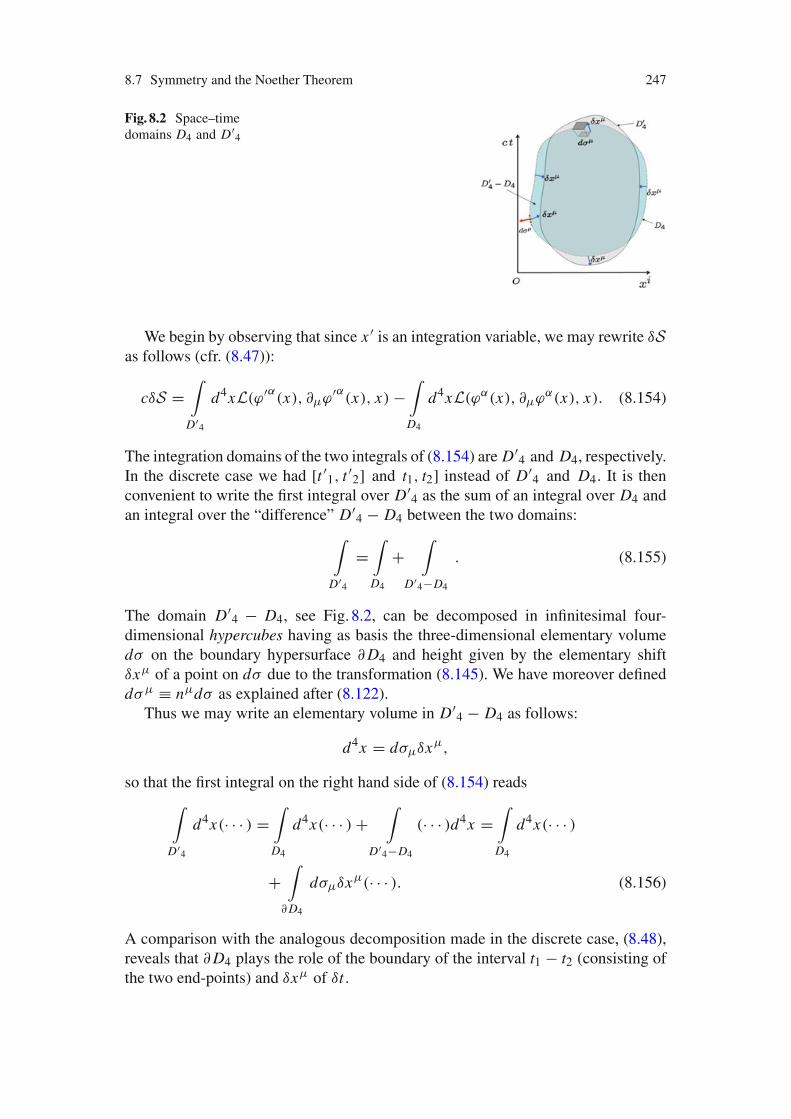
Fig. 8.2 Space–timedomains D4 and D'

4

We begin by observing that since x ' is an integration variable, we may rewrite %Sas follows (cfr. (8.47)):

c%S ="

D'4

d4xL("'#(x), $µ"'#(x), x) #"

D4

d4xL("#(x), $µ"#(x), x). (8.154)

The integration domains of the two integrals of (8.154) are D'4 and D4, respectively.

In the discrete case we had [t '1, t '2] and t1, t2] instead of D'4 and D4. It is then

convenient to write the first integral over D'4 as the sum of an integral over D4 and

an integral over the “difference” D'4 # D4 between the two domains:

"

D'4

="

D4

+"

D'4#D4

. (8.155)

The domain D'4 # D4, see Fig. 8.2, can be decomposed in infinitesimal four-

dimensional hypercubes having as basis the three-dimensional elementary volumed( on the boundary hypersurface $ D4 and height given by the elementary shift%xµ of a point on d( due to the transformation (8.145). We have moreover definedd(µ " nµd( as explained after (8.122).

Thus we may write an elementary volume in D'4 # D4 as follows:

d4x = d(µ%xµ,

so that the first integral on the right hand side of (8.154) reads"

D'4

d4x(· · · ) ="

D4

d4x(· · · ) +"

D'4#D4

(· · · )d4x ="

D4

d4x(· · · )

+"

$ D4

d(µ%xµ(· · · ). (8.156)

A comparison with the analogous decomposition made in the discrete case, (8.48),reveals that $ D4 plays the role of the boundary of the interval t1 # t2 (consisting ofthe two end-points) and %xµ of %t.


We may now insert this decomposition in (8.154) obtaining (see (8.51)):

c%S ="

D4

d4xL("'#(x), $µ"'#(x), x) #"

D4

d4xL("#(x), $µ"#(x), x)

+"

$ D4

d(µ%xµL("#(x), $µ"#(x), x), (8.157)

where, in the last integral, we have replaced L("'#(x), $µ"'#(x), x) with L("#(x),

$µ"#(x), x), since their difference, being multiplied by %xµ would have been aninfinitesimal of higher order (see the analogous equation (8.54)). On the other handthe difference between the first two integrals can be written as follows: (8.52):"

D4

d4x)L("'#(x), $µ"'#(x), x) # L("#(x), $µ"#(x), x)

*

="

D4

d4x#

$L$"#

%"# + $L$($µ"#)

%$µ"#

$

="

D4

d4x#

$L$"#

# $µ$L

$($µ"#)

$%"#(x) +

"

D4

d4x$µ

%$L

$($µ"#)%"#

&. (8.158)

where, as usual, we have applied the property

%($µ"#) = $µ%"#.

Finally we substitute (8.157) and (8.158) into (8.152) obtaining, for the variationof the action (see (8.53)):

c%S ="

D4

d4x#

$L$"#

# $µ$L

$($µ"#)

$%"#(x) +

"

D4

d4x$µ

%$L

$($µ"#)%"#

&

+"

$ D4

d(µ%xµL("#(x), $µ"#(x), x). (8.159)

If the Euler–Lagrange equations (8.121) are satisfied, the first integral in (8.159)vanishes; moreover the last integral can be written as an integral on $ D4 by use ofthe four-dimensional Gauss (or divergence theorem) theorem in reverse:

"

$ D4

d(µ%xµL ="

D4

d4x$µ(%xµL). (8.160)

We have thus obtained:

%S = 1c

"

D4

d4x$µ

#$L

$($µ"#)%"# + %xµL

$. (8.161)


The above equation gives the desired result: it states that when %S = 0, the integralin (8.161) is zero. Taking into account that the integration domain is arbitrary, wemust have:

$µ Jµ = 0, (8.162)

where

Jµ = $L$($µ"#)

%"# + %xµL. (8.163)

In terms of the infinitesimal, global parameters %,r , r = 1, . . . , g of the contin-uous transformation group G, the infinitesimal variations %"# and %xµ can bewritten as

%"# = %,r-#r ; %xµ = %,r Xµ

r . (8.164)

where -#r andXµ

r are, in general, functions of the fields "# and coordinates xµ. Thuswe may write:

Jµ = %,r Jµr ,

where

Jµr =

%$L

$($µ"#)-#

r + Xµr L

&. (8.165)

Taking into account that the %,r are independent, constant parameters, we can statethat we have a set of g conserved currents $µ Jµ

r = 0. To each conserved current Jµr

there corresponds a conserved charge Qr:

Qr ="

R3

d3xJ 0r , (8.166)

where we take as V the entire three-dimensional space R3. Indeed:

d Qr

dt= c

"

R3

d3x$

$x0 J 0r = #

"

R3

d3x$

$xi J ir = #

"

S*

d2(

3!

i=1

J ir ni = 0.

where the last surface integral is zero being evaluated at infinity where the currentsare supposed to vanish.


8.8 Space–Time Symmetries

As already stressed in the first Chapters of this book, in order to satisfy the princi-ple of relativity a physical theory must fulfil the requirement of invariance underthe Poincaré group. The latter was discussed in detail in Chap. 4 and contains, assubgroups, the Lorentz group and the four-dimensional translation group. Invarianceof a theory, describing an isolated system of fields, under Poincaré transformationsimplies that its predictions cannot depend on a particular direction or on a specificspace–time region in which we observe the system, consistently with our assumptionof homogeneity and isotropy of Minkowski space.

The Noether theorem allows us to derive conservation laws as a consequenceof this invariance. Let us first work out the conserved charges associated with theinvariance of the theory under space–time translations:

xµ ! x 'µ = xµ # *µ #! %xµ = #*µ,

"'#(x # *) = "#(x) ( %"#(x) = "'#(x) # "#(x) = $"#(x)

$xµ*µ. (8.167)

Comparing this with the general formula (8.164) we can identify the index r withthe space–time one µ, the parameters %,r with *µ and

-#r = -#

' = $µ"#%µ' ; Xµ

r = Xµ' = #%µ

' .

Requiring invariance of the action under the transformations (8.167), and insertingthe values of %xµ and %"# in the general expression of the current (8.163) we obtain:

Jµ = Jµ+ *+ =

%$L

$($µ"#)$+"# # %µ

+ L&

*+ " c*+T µ+ (8.168)

where we have introduced the energy-momentum28 tensor Tµ|+:

Tµ|+ " 1c

#$L

$($µ"#)$+"# # )µ+L

$, (8.169)

so that we have the general conservation law:

$µT µ' = 0. (8.170)

We note that both the indices of Tµ|' are Lorentz indices, but we have separatedthem by a bar since the first index is the index of the four-current while the secondindex is the index r labeling the parameters. This being understood, in the followingwe suppress the bar between the two indices of Tµ|' .

28 The alternative name of stress-energy tensor is also used.

8.8 Space–Time Symmetries 251

The four Noether charges associated with the space–time translations are obtainedby integration of J 0

µ " cT 0µ over the whole three-dimensional space.

Qµ = c"

d3xT0µ.= cPµ, (8.171)

and, from the Noether-conservation law $vT vµ, we obtain in the usual way that:

ddt

Pµ = 0.

To understand the physical meaning of the energy-momentum tensor and of theconserved four-vector

Pµ ""

V

d3xPµ ""

V

d3xT 0µ, (8.172)

where we have defined Pµ " T 0µ, we recall that in the case of systems with a finitenumber of degrees of freedom, the conserved four charges associated with space–time translations are the components of the four-momentum. It is natural then tointerpret Pµ as the total conserved four-momentum associated with the continuoussystem under consideration, described by the fields "#(x).

As a consequence of this the tensor Tµ' can be thought of as describing thedensity of energy and momentum and their currents in space and time. In particular,Pµ " T 0µ represents the spatial density of the four-momentum. We concludethat the four conserved charges Qµ/c associated with the space–time translations,which are an invariance of an isolated system, are the components of the total four-momentum.

Let us now consider the further six conserved charges associated with the invari-ance with respect to Lorentz transformations.

Under such a transformation, the fields "# will transform according to theSO(1, 3) representation, labeled by the index #, which they belong to; its infini-tesimal form has being given in (7.83), namely:

%"# = 12%,+(

7(L+( )#.". + (x+$( # x( $+)"#

8. (8.173)

If the action is invariant under the Lorentz group, substitution of the variations (8.173)and (7.82) into (8.163) gives the following conserved current:

Jµ = # c2%,+( Mµ|+( , (8.174)

where we have introduced the tensor:

Mµ|+( = #1c

#$L

$($µ"#)

3(L+( )#.". + (x+$( # x( $+)"#

4

++x( )µ+ # x+)µ(

,L

*, (8.175)


and used the identification of the index r with the antisymmetric couple of indices(µ') labeling the Lorentz generators, so that

Xµr " Xµ

+( = %µ+ x( # %µ

( x+,

-#r " -#

+( = (L+( )#.". + (x+$( # x( $+)"#. (8.176)

Comparing (8.175) with the definition of the energy-momentum tensor Tµ+ , (8.169),little insight reveals that the two terms proportional to xµ within square bracketsin the former can be expressed in terms of Tµ+ as x( Tµ+ # x+Tµ( . Therefore theconserved current Mµ|+( takes the simpler form:

Mµ|+( = ##

1c

$L$($µ"#)

(L+( )#.". + (x+Tµ( # x( Tµ+)

$. (8.177)

Being this current associated with Lorentz transformations which are always a sym-metry of a relativistic theory, the Noether theorem implies:

$µMµ+( = 0. (8.178)

Using the explicit form (8.177) in the conservation law (8.178) together with (8.170),we derive the following two equations:

$µHµ+( + T+( # T(+ = 0, (8.179)

$µTµ' = 0. (8.180)

where we have set

Hµ+( " 1c

$L$($µ"#)

(L+( )#.". .

While (8.180) yields again the conservation law associated with the energy-momentum tensor, (8.179) implies a condition that cannot be satisfied if Tµ' isnot symmetric in its two lower indices. To see this, let us consider the case of a scalarfield "(x) carrying no representation index # so that Hµ+( = 0. Then T+( #T(+ += 0would be inconsistent with (8.179) which is a consequence of the Noether theorem(8.178). Actually, as it is apparent from its definition, T +( is in general not a symmet-ric tensor, thus ruining the conservation law (8.178), which, as we shall show shortly,in particular implies the conservation of the total angular momentum. To solve thisseeming inconsistency we note that the definition (8.169) does not determine theenergy-momentum tensor uniquely. If we indeed redefine T µ' as:

T µ' ! T µ' + $+U 'µ+, U 'µ+ = #U '+µ (8.181)

it still satisfies the conservation law, since $µ$+U 'µ+ " 0, due to the antisymmetryof U 'µ+ in its last two indices. This possibility is related to the freedom we have of


adding to the Lagrangian a four-divergence $µ f µ. Although we had neglected suchfreedom when proving the Noether theorem, one can exploit it to obtain a symmetricenergy-momentum tensor.29 To show this, let us perform the following redefinitions:

/µ' = Tµ' + $0U'µ0; U'µ0 = #U'0µ, (8.182)

Mµ|+( = Mµ+( # $0+x+U(µ0 # x( U+µ0

,. (8.183)

where /µ' is the new energy momentum tensor. As already remarked these rede-finitions do not spoil the conservation law associated with the energy-momentumtensor, since, due to the antisymmetry of Uµ'0 in the last two indices, we stillhave $µ/µ' = 0. Moreover, by the same token, it is easily shown that Mµ|+(

is still conserved, i.e. $µMµ|+( = 0, since Mµ|+( is and the additional term$0

+x+U(µ0 # x( U+µ0

,is divergenceless by virtue of the antisymmetry of U(µ0

in its last two indices:

$µ$0+x+U(µ0 # x( U+µ0

,= 0. (8.184)

Let us now show that Mµ+( can be written in the simpler form:

Mµ|+( = #x+/µ( + x( /µ+, (8.185)

by a suitable choice of U(µ0. If we prove this, then, from the conservation of thecurrent Mµ|+( , we have

0 = $µMµ+( = #%µ+ /µ( + %µ

( /µ+ = #/+( + /(+, (8.186)

which implies that /µ' is symmetric. To prove (8.185) we first write the explicitform of Mµ+( by expressing Tµ' in (8.177) in terms of /µ' and use the followingidentity:

#x+$0U(µ0 + x( $0U+µ0 = #$0+x+U(µ0 # x( U+µ0

,# U+µ( + U(µ+ .

The four-divergence on the right hand side cancels against the opposite term in(8.183) and we end up with:

Mµ|+( = #Hµ+( # x+/µ( + x( /µ+ # U(µ+ + U+µ( . (8.187)

Thus in order for M to have the form (185) we need to find a tensor U'µ0 satisfyingthe following condition:

U+µ( # U(µ+ = 1c

$L$$µ"#

(L+( )#.". " Hµ+( . (8.188)

29 We shall illustrate an application of this mechanism in the case of the electromagnetic field.


The solution is30

Uµ+( = 12

)Hµ+( # H(µ+ # H+(µ

*. (8.189)

Let us now discuss the physical meaning of the conservation law (8.178), by com-puting the conserved “charges” Q+( associated with the 0-component of the currentMµ|+( (8.186). Let us rename Q+( ! J+( , since, as we shall presently see, they arerelated to the angular momentum. Then integrating over the whole space V = R3:

J+( ="

V

d3xM0+( = #"

V

d3x#

$L$"#

(L+( )#.". + (x+T0( # x( T0+)

$, (8.190)

are the conserved charged associated with Lorentz invariance:

ddt

J+( = 0. (8.191)

In particular for spatial indices (µ') = (i j) we find:

Ji j = #"

V

d3x#

$L$"#

(Li j )#.". + (xiP j # x jPi )

$= #*i jk J k, (8.192)

where P i is the momentum density.Let us first consider the case of a scalar field " which, by definition, does not

have internal components transforming under Lorentz transformations, so that thefirst term of (8.192) is absent. The second term in the integrand of (8.192) is easilyrecognized as the density of orbital angular momentum. Therefore Ji j " #*i jk Mk

is the conserved orbital angular momentum,which, for a scalar field, coincides withthe total angular momentum.

If, however, we have a field "# transforming, through the index #, in a non-trivialrepresentation of the Lorentz group, the first term in (8.177) is not zero; it is clear thatit should also describe an angular momentum which must then refer to the intrinsicdegrees of freedom of the field.31 In fact the first term describes the intrinsic angularmomentum or spin of the field.

In general if the field is not spinless the conservation law implies that only thesum of the orbital angular momentum and of the spin, that is only the total angularmomentum is conserved.

Note that so far we have been discussing the conservation of the three charges Ji jassociated with the invariance under three dimensional rotations and corresponding

30 The solution (8.189) can be obtained writing, besides (8.188), two analogous equations obtainedby cyclic permutation of the indices +µ(. Subtracting the last two equations from the first and usingthe antisymmetry property (8.181) we find (8.189).31 Recall from Chap. 4 that, since L+( are Lorentz generators, Li = #*i jk L jk/2 are generators ofthe rotation group.


to the components of the total angular momentum. It is interesting to understand themeaning of the other three conservation laws (8.178) associated with the invarianceunder Lorentz boosts, that is to the components J 0i of the Jµ' charges. Restrictingfor simplicity to the case of a scalar field, we have from (8.190) and (8.191), setting(Li j )

#. = 0,

ddt

#x0

"d3xT 0i #

"xi T 00d3x

$= 0. (8.193)

Taking into account the conservation of Pi , defined by the first integral, we obtain:

cPi = ddt

"xi T 00d3x. (8.194)

On the other hand since cT 00 represents the energy density, we have T 00d3x =d E/c = cdm, where E is the total energy related to the total mass by the familiarrelation E = mc2. It then follows:

P = ddt

"xdm. (8.195)

In words: The conservation law associated with the Lorentz boosts implies that therelativistic center of mass moves at constant velocity.

8.8.1 Internal Symmetries

The symmetries and the associated conserved charges discussed in the previous sec-tion are space–time symmetries, namely symmetries associated with translations andLorentz transformations under which, in a relativistic theory, the action is invariant.

We now want to give an example of a symmetry which does not involve changesin the space–time coordinates xµ, but that is rather implemented by transformationsacting on the internal index # of a field "#(x). In this case the index # labels thebasis of a representation of the corresponding symmetry group G. Such symmetriesare called internal symmetries and G is the internal symmetry group:

xµ ! x 'µ = xµ ( %xµ = 0,

"#(x) ! "'#(x) = "#(x) + %"#(x), (8.196)

where

%"# = %,r (Lr )#.". , %,r , 1.

From (8.163) the conserved currents have the simpler form:


%,r Jµr = $L

$($µ"#)%"#. (8.197)

The simplest, albeit important, example is the case in which we have two real scalarfields "1,"2, or, equivalently, a complex scalar field ","-, the two descriptions beingrelated by

"1 = 1.2(" + "-); "2 = # i.

2(" # "-),

and a Lagrangian density of the following form:

L = c2%

$µ"-$µ" # m2c2

!2 "-"&

. (8.198)

The Euler–Lagrangian equations are

!2$µ$µ" + m2c2" = 0. (8.199)

As will be shown in the next Chapter this equation is the natural relativistic extensionof the Schrödinger equation for a particle of mass m and wave function ". It is referredto as the Klein–Gordon equation, and the Lagrangian (8.198) is the Klein–GordonLagrangian density.

We observe that the Lagrangian density L of (8.198) is invariant under the fol-lowing transformation:

"(x) ! "'(x) = e#i#"(x) (8.200)

where # is a constant parameter.In the real basis, the transformation belongs to the group SO(2):

%"'

1"'

2

&=

%cos # sin #

# sin # cos #

& %"1"2

&. (8.201)

In the complex basis the transformation (8.200) defines a one-parameter Lie groupof unitary transformations denoted by U(1), which is isomorphic to, i.e. has the samestructure as, SO(2). The infinitesimal version of (8.200) is

"(x) ! "'(x) / "(x) # i#"(x) ( %"(x) = #i#"(x); %"- = i#"-.

Using a suitable multiplicative coefficient to normalize the conserved current Jµ tothe dimension of the electric current, we obtain from (8.197):

# Jµ = ec!

#$L

$($µ")%" + $L

$($µ"-)%"-

$= #i

ec!

)"$µ"- # "-$µ"

*#. (8.202)

Let us verify the conservation law $µ Jµ = 0 explicitly:


i!ec

$µ Jµ = $µ"$µ"- + "$µ$µ"- # $µ"-$µ" # "-$µ$µ"

= m2c2

!2 ""- # m2c2

!2 ""- = 0

where we have used the equation of motion (8.199). We shall see in Chap. 10 thatthe conserved charge:

Q ="

d3xJ 0 = ie!

"d3x("-$t" # "$t"

-) (8.203)

can be identified with electric charge of a scalar field " interacting with the electro-magnetic field.

Let us note that if the field were real, "(x) = "-(x), that is if we had just one field,there would be no invariance of the Lagrangian and the charge Q would be zero. Asit will be shown in the sequel, this is a general feature: when a field is interpreted asthe wave function of a particle, a real field describes a neutral particle, as it happensfor the photon field Aµ(x) = A-

µ(x), while fields associated with charged particlesare intrinsically complex.

8.9 Hamiltonian Formalism in Field Theory

In the previous section we have described systems with a continuum of degrees offreedom using the Lagrangian formalism. We want now discuss the dynamics ofsuch systems using the Hamiltonian formalism. The most direct way to derive theHamiltonian description of field dynamics is to use the limiting procedure discussedin Sect. 8.5.1 for the Lagrangian formalism

Consider a theory describing a field "(x) (let us suppress the internal index #

for the time being). Just as we did in Sect. 8.5.1, we divide the three-dimensionaldomain V in which we study the system, into tiny cells of volume %V i , defining theLagrangian coordinates "i (t) as the mean value of "(x, t) within the i th cell. Wethus have a discrete dynamic system and define the momenta pi conjugate to "i as

pi = $L(t)$"i (t)

. (8.204)

The Hamiltonian of the system is given by

H =!

i

pi "i # L , (8.205)

with equations of motion:

"i = $ H$pi

; pi = #$ H$"i

. (8.206)

Recall now from the discussion in Sect. 8.5.1 that, in the continuum limit (%Viinfinitesimal)

Documents

8.5 Lagrangian and Hamiltonian Formalism in Field Theorieszwirner/DT-ch8parte.pdf · 2014-01-09 · 8.5 Lagrangian and Hamiltonian Formalism in Field Theories 233 on the values of