88-051

CONTROLLING A STATIONARY ORBIT USING ELECTRIC PROPULSION

Bernard M. Anzel, Laboratory Scientist

Hughes Aircraft CompanySpace and Communications Group

Systems LaboratoriesEl Segundo, California, U.S.A.

ABSTRACT For thrusters using electric propulsion the thrustlevels are on the order of millipounds so corrections must

The system proposed consists of two ion engines be made more often. Furthermore, the thrusting time formounted on the antinadir face of a satellite. Each engine liquid propulsion is usually less than 2 minutes so the burnis fired once per orbit sidereal period, and automatically is essentially impulsive. The low thrust level associatedprovides acceleration components to correct the inclina- with electric propulsion results in a longer thrustingtion, eccentricity, and drift parameters of a stationary orbital arc, which is less efficient. However, the orbitalorbit. arc over which thrusting occurs may be minimized by

Both engines are canted 8° away from the antinadir maximizing the correction frequency.

face. One engine is primarily thrusting north, and the

other south. To control orbit inclination, the south A significant advantage of electric propulsion over

thrusting engine is fired over an arc centered about a liquid propulsion is the much higher (-3000 versus

right ascension of 900; the north thrusting engine is fired 200 seconds) specific impulse. This is particularly bene-

over an arc centered about a right ascension of 2700. For ficial in correcting orbital inclination, which requires

equal burn arcs the radial acceleration components are almost a the velocty needed for stationkeepig. The

equal so that no net change is eccentricity results. The optimum point in space for correction of orbital iclina-

use of unequal burn arcs, however, results in partial tion is about 270 relative to Aries (see "Orbital

eccentricity control.Analysis") for positive velocity increments and 90 fornegative velocity increments.

If the ion engines may be swiveled to about thenorth-south axis, tangential components of acceleration Making two corrections per day as opposed to one

will result upon thrusting. These are used to control doubles the inclination correction frequency but requires

satellite drift along with some eccentricity control. The two ion thrusters instead of one. The increased

magnitude of a depends on the satellite station longitude, flexibility provided by two thrusters permits control of

precession of the orbit plane caused by solar-lunar orbital semimajor axis and eccentricity in addition to

gravity, and the cant angle of the engines. inclination. This is the crux of the concept presented inthis paper.

Control of satellite drift and orbit inclination is very

tight, while control of orbit eccentricity is limited by the 2. ION THRUSTER CONFIGURATIONrequirement that the engine firings are fixed in space.

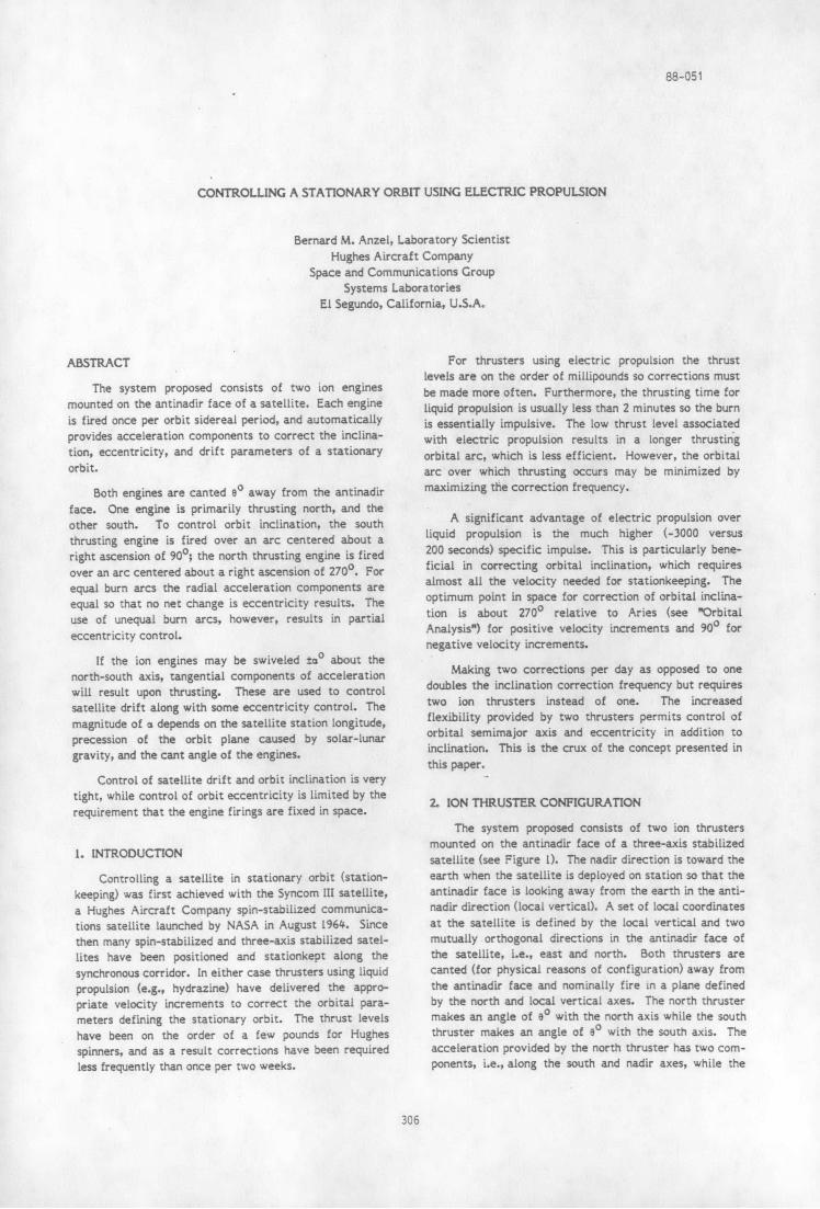
The system proposed consists of two ion thrustersmounted on the antinadir face of a three-axis stabilized

1. INTRODUCTION satellite (see Figure 1). The nadir direction is toward the

Controlling a satellite in stationary orbit (station- earth when the satellite is deployed on station so that the

keeping) was first achieved with the Syncom III satellite, antinadir face is looking away from the earth in the anti-

a Hughes Aircraft Company spin-stabilized communica- nadir direction (local vertical). A set of local coordinates

tions satellite launched by NASA in August 1964. Since at the satellite is defined by the local vertical and two

then many spin-stabilized and three-axis stabilized satel- mutually orthogonal directions in the antinadir face of

lites have been positioned and stationkept along the the satellite, i.e., east and north. Both thrusters are

synchronous corridor. In either case thrusters using liquid canted (for physical reasons of configuration) away from

propulsion (e.g., hydrazine) have delivered the appro- the antinadir face and nominally fire in a plane defined

priate velocity increments to correct the orbital para- by the north and local vertical axes. The north thruster

meters defining the stationary orbit. The thrust levels makes an angle of es with the north axis while the south

have been on the order of a few pounds for Hughes thruster makes an angle of e9 with the south axis. The

spinners, and as a result corrections have been required acceleration provided by the north thruster has two com-

less frequently than once per two weeks. ponents, i.e., along the south and nadir axes, while the

306

NORTH

RGNORTH NADIRTHRT NA

ASCENSION-90

RRIGHTHT

ASCENSION . 270

Fig. 1: Ion thruster configuration.

acceleration provided by the south thruster has two com- error will cause the orbit of a "stationary" satellite to

ponents along the north and nadir axes. wander about or drift away from the perfect orbit.

To provide the flexibility for orbit control discussed Let the reference position of a stationary orbit be at

in this paper, the capability to swivel the ion thrusters synchronous radius and on the equator positioned over a

about the north-south axis must exist. The projection of desired longitude; then the relative motion of a near sta-

the force vector into the plane defined by the local verti- tionary orbit can be described by its longitudinal (east-

cal and east axes would then be tao away from the nadir west) and latitudinal (north-south) angular variation in

direction, resulting in tangential acceleration. Thus all addition to a radial (toward or away from the earth)

three components of acceleration, i.e., north-south, east- variation. From linear theory the equations describing

west and radial, would be present upon thrusting. this motion are,

3. ORBITAL ANALYSIS 2rir = - d - r e cos (u t)

This section provides a cursory summary of the 3 We s e

mathematical technique (Ref 1) necessary to perform the

orbital analysis for the concepts presented in this paper. 6 -* dt + 2e sin (w t) (1)e

3.1 Near Stationary Orbits6 * i sin (ea c * )

A stationary orbit is one whose satellite track on the

earth is a point on the equator that does not move. This (c - 0, perigee)

requires that the satellite orbit be circular (eccentric-

ity = 0), equatorial (inclination = 0), and possessing a

period equal to that of the earth's rotation. A stationary where Sr, 6X, 6 are relative radius, relative longitude

orbit is a fiction in practice, since various sources of and latitude respectively; longitude is positive east.

307

d = mean drift rate 3.3.1 Earth Triaxiality - Effect on Drift Vector

e orbit eccentricity A nominally stationary satellite will tend to driftfrom its longitudinal position mainly because of a long-

i = orbit inclination term tangential pertubing force due to the earth'striaxiality or elliptical shape of the earth's equatorial

S = earth rate section. The result is a longitudinal acceleration which isa function of the longitude of the satellite. This acceler-

r = synchronous radius ation is plotted in Figure 2 in deg/day 2 versus longitudeusing a positive east sign convention. There are four

S = argument of perigee longitudes around the equator where the acceleration iszero. The maximum acceleration of about 2 x 10"

deg/day2 occurs at a longitude of -120 0 E. Tightly

3.2 Definition of Vector Elements stationkept satellites maintain longitude within ±0.05o sothat the longitudinal acceleration is virtually constant.

The classical elements used to define an orbit are Thus the vector drift coordinates vary simply assemimajor axis (a), eccentricity (e), inclination (i), meananomaly (M), argument of perigee (w), and right ascension d = d * At (3)of ascending node (0). The vector elements are definedin terms of the classical elements by tI L d t + 1/2 At2

o o

where A = constant drift acceleration= [l-l5,d] = drift vector (2)

S khl ] exp j (w ) Ltd o 2 initial values of vector drift coordinatese = [kl'hl] = e exp j (u + a)

3.3.2 Sun/Moon Gravity and Earth Oblateness - Effect onS = [k2 ,h2 ] =I exp j (a) Inclination Vector

2-. = relative mean longitude It can be shown using advanced methods (Ref 2) thats the long-term motion of 1, a unit vector in the direction

t = S - GHA (t s = reference stationary longitude) of the satellite orbit normal is of the form

S =M+ + a 2= - E ,. (ft . .) (. X ) (4)

CHA = Greenwich hour angle of Aries j=0

d =.where S0 , fi, and S2 are unit vectors in the directions

e = cos 0 + j sin 4 of earth's polar axis, pole of the ecliptic and moon's orbitnormal respectively. For the jth term, the motion repre-

hi e sin (w + a) sented would be a precession of I about . at a constantrate c. (1- .) . Thus, the motion of I Is described as

k = e cos (wn + ) simultaneous precession about three axes. Oblatenesstends to precess the orbit normal about the earth's polar

h2 = i sin (a) axis, solar gravity precesses it about the pole of the

k2 = i cos (a)

For near stationary orbits, S is to first order, the meanright ascension of the satellite at the time t. The 1abscissae (either k or k2 depending on which element is

being considered) is the direction of Aries, the referencefor the right ascension S. ej* is a unit vector makingangle i with abscissae. __

3.3 Perturbations

Perturbations on a stationary orbit result from -

external forces which change the orbital elements. The

exact manner in which these forces alter the orbital ele-

ments is a complex problem which does not lend itself tosimple mathematical models. However, the major effect 0 40 80 120 160 200 240 280 320 360

of the perturbation on each vector element can be EAST LONGITUDE, DEGapproximated. Fig. 2: Logitudinal acceleration

308

ecliptic, and lunar gravity precesses it about the pole of where

the moon's orbit. The pole of the ecliptic may be

considered to remain inertially fixed with an inclination t0 = spring equinoxof 23.440 to the earth's polar axis. Although the pole ofthe lunar orbit is inclined 5.150 to the pole of the eclip- t-to = fraction of a yeartic, its direction is constantly changing as it precessesabout the pole of the ecliptic with a period of 18.6 years. u = 2r rad/year

Assuming an equatorial satellite, the long term ; 3r rad/dayvariation of the inclination vector coordinates is se m

approximated by (Ref 3) Vs = synchronous velocity

h2 0.852 + 0.098 cos A (5) solar force to spacecraft mass ratio2 a

deg/year

k -0.132 sin A 3. Impulsive Velocity Corrections2 m

Assume an impulsive velocity correction

where A is the longitude of the ascending node of the '= (AVg, AV'T, V) where R, T, and N are radial,

moon's orbit on the ecliptic and tangential, and normal components in a local coordinatesystem at the satellite as defined previously; i.e., radialis local vertical, positive tangential is east, and positive

A 2- (t - ), - t in years, Mar 1969 normal is north. Let the point of application of a be atin 18.6 ( - o) - o in yar, o

a mean right ascension SA; then

There are also periodic variations in these 3 1coordinates. The most significant results from the varia- = 2 -VR, V ytion in the declination of the sun and varies at twice sun s s ()frequency or 4w radians per year. The variation of the

vector inclination can be approximated by a rotating vec- 2 AVT Vtor of constant magnitude so that (Ref 4) exp (jSA) - j exp (jS A

s s

h (2S) x -0.28 cos [2w (t-t)] AV Y S2(6) 0 eip (iS.A)

deg/year

k2 (2S) * 0.28 sin [2ws(-to)] It is seen that L may be changed only by a suitableradial velocity impulse and d changed only by a suitable

where tangential velocity impulse. The changes in l or d areindependent of the point of application of the particular

t = spring equinox impulse. Only a normal component of velocity incremento will change the inclination vector and the change induced

t-t = fraction of a year is in a direction given by the mean right ascension SA atSthe point of application. A given Ie is produced by

w = 2w rad/year either a tangential velocity impulse applied at SA or as radial velocity impulse of twice the magnitude applied

90° away. It is also seen that any impulsive change in a

3.3.3 Solar Radiation Pressure - Effect on Eccentricity wil cause a change in and conversely.

Vector

When radiation from the sun strikes the surface of a 4. THRUSTING WITH ELECTRIC PROPULSION

satellite, it imparts a pressure on the surface. This pro-f a continuous thrust is applied to a stationary orbitduces an acceleration which acts along the sunline and

over an arc WT- (Tp = thrusting time) in a northerlyresults in a mean daily change in the vector eccentricity over an arc (T = thrusting time) in a northerly

direction, then the magnitude of the inclination change(Ref 4) of magnitude proportional to the solar force to direction, then the magnitude o the inclination change

spacecraft mass ratio and in a direction perpendicular to Tthe sunline and leading it. This variation at sun ffrequency of the ecentricity vector coordinates is then 6i . cos (we) dt (9)(assumes constant | ) P s P

2

whereh Cos WI s o (c - C) (7)

aVp = total velocity increment over time Tp

. = -e l sin ws (t - t0 ) AVp/Tp = acceleration

309

ue Tp\ accordance with 3.4, a radial AV affects both the vector. Vp sin -J eccentricity and the vector drift. The radial AV at the

S V (0) R.A.= 90° firing is negative, thereby producing

-a e directed toward R.A. = 1800. The radial AV at theR.A. = 2700 firing is also negative but produces

sin (e Tp/2)/(e Tp/2) can be considered an efficiency ae directed toward R.A. = 00. If the magnitudes of thefactor on AVp so that for mathematical purposes the radial components are equal then the net change in e isimpulsive theory applies, zero. The Xe exists before it is cancelled by the second

firing 12 hours later. The peak of the diurnal variation inAlso longitude (2e) during this period is about 0.00150.

mAVP (F cos e) T (11) In the case of the vector drift a secular growth inthe mean longitude coordinate occurs since the radial

m = spacecraft mass components are of the same sign. The magnitude of thismotion is proportional to the magnitude of the

F = force from ion thruster N-S AV required to counter the perturbation. If therequired N-S corrections each day were constant then the

e =thruster cant angle mean longitude shift per day would be constant. Thismay be compensated for by initializing the orbitsemimajor axis to a value deviated from synchronous

Ai. (12) radius in order to produce a steady longitudinal driftexactly equal and opposite to the shift in mean longitudeproduced by the radial components.

where

Therequired N-S AV corrections are not constantS1/2 because t due to the perturbation is not constant

| = 1( )2 + ( 2) deg/year (3.3.2). To correct this variation the ability to alter thesemimajor axis and thus the mean drift rate must exist.This equates to the ability to produce tangential velocity

Substituting (11) for AVp into (10), and (12) for Aip increments.into (10) with we = 0.7292 x 10 4 rad/sec, Vs =10087.47 fps. 6. CONTROLLING DRIFT

, .If an ion engine may be swiveled about the N-S axis

si ("e 8.9 X 10 6 (13) so that the projection of its thrust vector in the orbitalz2 1 cos a

plane makes an angle ±a with the nadir direction, then atangential component of acceleration will result upon

As an examplq, consider only the long term variation thrusting. This will permit altering the orbit semimajor

of inclination; if II = 0.95°/year, e = -300, m = 80 slugs, axis in a manner required to correct variations in thedrift vector.and F = 2.2 millipounds, then the thrusting arc we T =

410, and the efficiency factor is 97.9 percent.6.1 Control of Mean Longitude Shift

5. CONTROLLING INCLINATION .Assume an average rate of change of inclination

Inclination is controlled by producing rates of change of to which the orbit semimajor axis is initialized so

of the vector inclination in a direction opposite to that that only variation above or below need be compensated

produced by the perturbation. As shown in 3.3.2 for the for by using tangential acceleration. Let SAVR be the

long term effects, this direction is mainly along h2 or 90o average daily radial velocity difference resulting from

from the Aries reference. Thus the direction of the the variation in I (deg/year), which shall be called St.

correction tmust be opposite this or 2700 from the Aries The relative mean longitude shift per day is at and

reference. According to equation (8) in 3.4, this can be2 180

accomplished by providing positive acceleration at a right at - ( - , deg/dayascension of 2700 or negative acceleration at a right S (14)ascension of 900, or both. The system proposed uses twoion thrusters as previously introduced. The north thrusterproduces negative acceleration so that its firing arc will sa ai ( 1be centered at R.A. = 900 while the south thruster V tan 0 365.25 180

produces positive acceleration so that its firing arc willbe centered at R.A. = 2700. For the long term a( \effects I = 0.950/year so that the maximum daily s -2 tn i (16)

latitude is 0.000650, which is very small.

5.1 Radial Coupling The method of control assumes that a = 0 for rdays so that the mean longitude shift builds over this

Due to the cant angle, a component of radial period of time. Then the angle a is commanded to aacceleration is produced during thruster firing. In desired value which introduces a daily change to the

310

change is reduced to zero. By centering the maximum

change about a nominal station longitude .

ST the (l - l ) peak can be reduced to 0 .0 0 8 8 5 °. The-- t(days) latter can be further reduced by decreasing T.

k-- Tda-*-ldy-) IINIAUZED TO i 6.2 Control of Mean Longitude AccelerationNOTE: Aa DRIFT ACCELERATION INDUCED BY SWIVEL ANGLEa (deg~a2)

Fig.3: Driftconrolcycle It was stated in 3.3.1 that the earth's triaxialityproduces a drift rate change or a mean longitude

mean drift rate, 6i, in a direction to reverse the mean acceleration which is a function of the satellite

longitude motion. This angle is maintained for T/2 days, longitude. The tangential velocity increments resulting

whereupon the angle a is commanded to a value equal but from swivelig the thrusters, and used for control of

opposite in sign so that the drift rate may be reduced mean longitude shifts in 6.1, can also be used to counter

symmetrically to its original value at a time T/2 days the effects of earth triaxiality. Two methods will be

later. At this time the angle a is commanded back to discussed. The first uses the same technique as discussed

zero and the cycle is repeated. Figure 3 illustrates the in 61. This method is concerned only with the day to day

drift control cycle. motion. The second method attempts to control the intra

day motion, i.e., between the two maneuvers 12 hoursThe mean longitude change resulting from the a apart.

induced drift acceleration is given by6.2.1 Method I

A T26, = (17) As in 6.1, for r days the angle a is zero so that the

S 4 mean longitude drifts under the action of triaxiality atotal of 1/2 AT where A = mean longitude acceleration

Based on the criterion that at the end of one deg/day 2 . The angle a is then commanded on, negative,cycle (T + T) , the mean longitude will have returned to and off in a period of T days. Based on the criterion thatits initial value. at the end of one cycle (r + T) the mean longitude will

have returned to its initial value.

S-2 Lan a ( + T) AT 2

4 6 -(18) 4 ~ 2 A ( + T) 2 0 (22)

3w Substituting for A from (19) and (20)a AV T = -0.10706 (AVT),

(19) . 38.75 A _ T (2 3sin a = an 7 T (23)

AVT fps/day

Minimum a occurs when T = 0 then

AVT = Vs tan e sna () 38.7 A38.75 A

(20) sin a ( -Fn (24)

Substitu ) io () ad tn i ) which is independent of the duty cycle and for thisSubstituting (20) into (19) and then into (18)

special case A - 2A. Figure 4 illustrates this cycle.

i (4 + T) Assume that only the long term effect on inclinationsin a = -0.4244 is t.o be controlled; then the maximum a will occur

S T (21) for I = 0.750/year and at the worst longitudewhere A x 2 x 10- eg/day2 . For 0 = -300 |a I =10.30.

Assume only the long term effect on inclination, e.g.

Sr For this value of A, and T = 14 days,S05/year the (t - as) peak is 0.033°. This is rather large and can

i = 0.10/ear be reduced by decreasing T. I max cannot be madesmaller unless the satellite operating longitude

corresponds to smaller values of triaxial acceleration (seeS = 56 days

Figure 2).

T =14 days

lal =1.020S/ \Aa T

In the above example the mean longitude changes in 7 -(days)

one direction by 0.01770 over the 56 days when a = 0. -Tdys--.-T days.---

Over the next 14 days of a control, the mean longitude Fig. 4: Drift control cycle

311

6.2.2 Method2 b 1 8AV Ib V t a n 9 s i n a

Let a be initialized at predetermined values for each Tb 365.25 180 s/

of the two ion engines, i.e., north and south.

The a values will be updated periodically by ground I and Ib refer to the amount of inclination correctioncommand as I varies with time. Assume that at t = 0, to be allocated to each thruster. They need not be equalthe cycle begins with the north thruster delivering enough as long as + I = I on a per day basis. Substitutingtangential AVT to reverse the mean drift rate from its (26) into (25) and solving for aa and abvalue at t = 0" to an equal and opposite value at t = 0

which begins the soft limit cycle (see Figure 5). During

the following 1/2 day, the mean longitude acceleration sin a 12.92 A (27)acts to reduce the mean drift rate until the satellite a tan e

mean longitude reverses. The time of this occurrence is

at t = 1/3 day. At t = 1/2-, the mean drift rate has sin ab 6.46 A

reversed; the south thruster, at t = 1/2 day, delivers b a benough AVT to once again reverse the mean drift ratefrom its value at t = 1/2" to an equal and opposite value if ib = 4i' then a - 2aat t = 1/2+. The satellite mean longitude reverses at the a a b

same longitude as occurred at t = 1/3 day but now at atime t= 2/3 day. The satellite then continues to If I 21 (. 2 i i . aaccelerate until t = I- when the north thruster will fire to a b a 3 b ' a b

repeat the cycle.

With this method, the tangential AV1 produced by Considering only long term perturbations on inclina-

one of the ion thrusters is twice as large as the tion, the maximum a will occur for I = 0.750 /year and at

produced by the other. In the above text it was assumed the worst longitude where A = 2 x 10 deg/day. For a

that the north thruster applied the larger VT . Either = - 3 0 0 and i = b' I amax = 6.850.

the north or south thruster can supply the larger AVr for For this value of A the (l - ts) peak is = =mean longitude control with the same result; however, 0.000110, which is exceedingly small.the phasing becomes important with regard to controlling

eccentricity, as will be discussed later. When using Method 2, the mean longitude shift dueto differential radial coupling may be compensated for

As seen in Figure 5, the required drift rate change simply by changing na and ab to produce the change infrom t = 0- to t = 0 + is -2A/3°/day while the change from drift rate required. This means, using equation (16) andt = 1/2" to t = 1/2 is -A/3 0 /day. The corresponding equation (26)tangential velocity increments are

-2 tan i 3we i a,bS A365.25 V 365.25 180

VTa -= 9.34 fps/day 365.25 a,b 365.25 (28)(25)

V s , V tan 9 sin a ,V . - 3- = 9.34 )ps/day s a,b

where the a and b subscripts refer to the larger and Approximating sin ea,b . a,b

smaller tangential velocity increments respectively

S 60 b deg (29)i a,b 2 deg

A a tan 9 sin a 'a,bT 365.25 180/ a (26)

which is the change required to compensate for radialcoupling; referring to the example above with 6 Ta,b

t0 0.05/year, i, = 0.375 0 /yearo^ + 1a,b

S RELAIVESd= MEANLONGITUOE(I-Is) a -0.81

S (+ EAST) a,b

Sr- 7. CONTROLLING ECCENTRICITY

-A The tangential velocity components generated by the

t/\ / -'I"T ACCELERATION (A) swivel angle a are used to control drift as discussed inAo

1 -2- 6.2. However, the eccentricity vector is also affected in3 1-,-o a manner given by equation (8) in 3.4. If the tangential

Fig. 5: Drift control soft limit cycle velocity components one-half orbit apart are equal, then

312

the net change in eccentricity I = 0; e exists before ih1 should be negative, and conversely for the other

it is cancelled by the second firing 12 hours later. The 1/2 year. Thus

peak of the diurnal variation in longitude (2e) during thisperiod is only about 0.004° for the Method I case of 2wf6.2.1. 6h1 (6.4 X 10 6 ) cos (w C) dt -

- Z (33)If the tangential velocity components one-half orbit s

apart are not equal, a secular growth in I will result.

Since the firings are centered near R.A. = 2700 and

R.A.= 90 o and the i direction will be along ±h 1. Thus (1.23 x 10- 6 )only the h, component of e due to solar radiation "s

pressure can be affected with the differential tangential

velocity components. The 1 component of a due to

solar radiation pressure can be affected using differential h L [2 (6.4 10-6 ) - .(1.23 x 10- 6

radial velocity components. s (34)

7.1 Controlling hi W = 0.0172 rad/day

This section will illustrate, by example, how h. maybe partially controlled using differential tangential 6h = 5 .2 x 10

velocity components. Method 2 described in 6.2.2 is

chosen since the AVT and AVT bear a distinctive By centering the hi motion about zero, h1 = 2.6 x 10

a b maxrelationship to one another and therefore &Ah isrestricted to This corresponds to a peak diurnal variation in longi-

tude of 2h = 0.030. If there were no counteringmax

2L - AV - (V3 rad/dy of i 1 from the differential tangential velocity incre-Ah - AV T TVb rad/day

a (30) ments, 2h = 0.043°. Since h is proportionalmax

to the triaxial acceleration A, then as A decreases sosubstituting (25) into (30) does and therefore the ability to reduce shl.

When A1 reverses sign, i.e., from t = r/2ws to&h = ±0.6173x 10- rad/day (31) t = 3w/2w s , the application R.A.s for &VTa and AV are

switched.

for A = 2 x 10- 3 deg/day 2

7.2 Controlling k1

Ah .= 1.23 x 10- 6 rad/day This section discusses how k1 may be partially- controlled using differential radial velocity components.

The to solar radiation pressure The north thruster produces a radial velocityThe h, component due to solar radiation pressure

Si i component which negates the change in eccentricityhas been approximated by equation (7) in 3.3.3 as

caused by the radial velocity component produced by thesouth thruster, if the amount of inclination correction

= s (c - cO ) (32) allocated to each thruster is equal. The north and southSs 0 thrusters may fire over unequal arcs producing unequal

amounts of inclination correction, but maintaining the

where required sum equal to the per day rate of change ofinclination produced by the perturbation. In this case,

l| = 12.81 rad/dayi I ib .= (35)

F force (pounds)M mass (slugs) (. .

8 a * 365l . -( tan 8, rad/day (36)Assume, e.g., F = 40 x 10-6 pounds, M = 80 slugs

Equation (36) arises from the unequal radial velocity

lel| 6.4 x 10- 6 rad/day components resulting in a secular growth of Ae. Sincethe firings are centered near R.A. = 2700 and R.A. = 900,the Ae direction will. be along tkl. Thus only

From t = - t/2u- (winter solstice) to t = + w/2w the . component of e due to solar radiation pressure

(summer solstice) h, is positive. During this period can be controlled with differential radial velocity

313

components. The k1 component has been approximated TABLE I. ECCENTRICITY CONTROL EXAMPLE

by equation (7) in 3.3.3 as control Parameters

R.A. R.A.(37)a pulse, b pulse, as - | in w s ( c -t ) (3 7 ) u n i , k a a" * - a

Ssin ( (37) Quadrant I 1 dog dse a b deg deg

From t = 0 (Vernal Equinox) to t = rl s (Autumnal I + - 270 90 ia -5.74 -3.19

Equinox) il is negative. During this period i&k should

be positive, and vice-versa for the other i year. Thus, 2 - - 90 270 i < -6.38 -2.87

assume, e.g., that I= 0.850 /year ; also that ak1 in

equation (36) is equal to t1.23 x 10-6 rad/day, the same3 - 90 270 1 > 1 -5.74 -3.19

value calculated for Ahl, in 7.1. This will allow a

for kI = 2.6 x 10 and a peak diurnal variation inmax 4

+ + 270 90 1 < -6.38 -2.87

longitude of 2k 1 = 0.03. Solving simultaneously frommax

(35) and (36), either ascension of the center of the firing pulse; one column isfor the a pulse and the other for the b pulse. The nexttwo columns show the relative magnitudes of inclination

ia * 0.4473, Ib 0.4027 correction required from each pulse. Using the results ofthe calculation performed in 7.2, the last two columns

or deg/year are the computed swivel angles required for the a and bpulses.

a 0.4027, Ib I 0.4473 It should be noted that control of hl is limited onlyby the magnitude of the triaxial acceleration while

is the solution depending on the time of year. If control of kI may be limited by the relative size of iis the solution depending on the time of year. If The choice of the latter will, however, a

more ki cancellation is desired, the difference between and ib T he c h oic e of t h e la t t er w ill, ho w ev e r , a f f ec t

Ia and b can be made larger. the sizes of na and ab"

7.3 Controlling hi and kiREFERENCES

Assume the use of Method 2 in controlling , and1Assume the use of Method 2 in controlling 1. Balsam, R. E. and Anzel, B. M., "A Simplifiedlet the a and b subscripts refer to the larger and smaller Approach for Correction of Perturbations on a

Approach for Correction of Perturbations on atangential velocity increments, respectively. Also Stationary Orbit," AIAA 2nd Communicationsassume, e.g., that the acceleration due to triaxiality is Satellite Systems Conference, San Francisco, CApositive and maximum. Let the reference time of year April 8-10, 1968.be zero at the vernal equinox and divide the year intofour quadrants: 2. Allen, R. R. and Cook, G. E., "The Long Period

Motion of the Plane of a Distant Circular Orbit,"

I) Vernal equinox - summer solstice Proceedings of the Royal Society, Vol 280, 1964.

2) Summer solstice - autumnal equinox2) Summer sol e - a l e x 3. Balsam, R. E., "Motion of the Orbital Plane of Near-3) Autumnal equinox - winter solsticeSAutumnal equinoxwinter solstice Stationary Satellites," IDC 2281, Hughes Aircraft4) Winter solstice - vernal equinox Company, March 1966.

Table I illustrates for each of these quadrants the 4. Anzel, B. M., "Orbital Dynamics for Synchronoussign of the i1 and k 1 produced by the solar radiation Missions," Training Manual, Hughes Aircraftpressure perturbation. Also indicated is the right Company, March 1982.

314