Embed Size (px)
Citation preview
F DAG12 891 AIR FORCE GEOPHYSICS LAB HANSCOMV AFB MA F/G 3/2
AN OBJECTIVE METHOD FOR FORECASTING SOLAR FLARES.(U)
FEB 81 D F NEIDIG, P H WIBORG, P H SEAGRAVES
UNCLASSIFIED AFGLTR-81-026ZS
S//AFGLTR-81-0026 . -
41WIlRONiMENTAL RERHPAP! RSdO. 726
/ An Objective Methodfor Forecasting Solar Flares,
,-ONALDAiEIDIG
/0 IHILIP J.IwIBORG.- AUL H./4EAGRAVES k\ JOSEPH V. .4IRMANWILLIAM E.LOWERS
4 Feb" M Qll81 Q
Approved for public role*"e; distribution unlimited. rECTE
SPACE PHYSICS DIVISION PROJECT 2311 j "Q -AIR FORCEr GEOPHYSICS LABORtATORY . ' >
G.7 HANSCOM APB. MASSACHUSETTS 01731
La. AIR FORCE SYSTEMS COMMAND, USAF
* j ~81 8 7 MR
This report has been reviewed by the ESD Information Office (01) and isreleasable to the National Technical Information Service (NTIS).
This technical report has been reviewed andis approved for publication.
FOR THE COMMANDER
,
C ef Scientist
Qualified requestors may obtain additional copies from theDefense Technical Information Center. All others should apply to theNational Technical Information Service.
UnclassifiedSECURITf CLASSIFICATION O
F THIS PAGE (Whon D*ta F-Pfled)
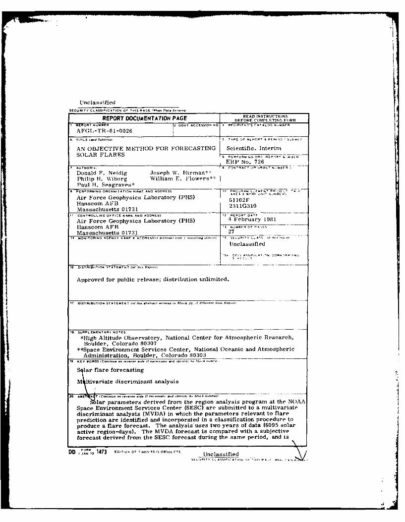
REPORT DOCUMENTATION PAGE READ INSTRUCTIONSBEFORE COMPI.ETINC, FORM
" REPORT NUMBER 12 GOVT ACCESSION No 3 RECIPIENT'S
CATALOG NUMBER
AFGL-TR-81-0026OE
4. TITLE ( d Subtst1I. 5 TYPE OF REPORT' & P[R,CT " 'E.) l
AN OBJECTIVE METHOD FOR FORECASTING Scientific. InterimSOLAR FLARES PERFORMNG ORC REPYRT N UBEQ
ERP No. 7267 AUTHOR, A CONTRACY oP RAN' N-MER
Donald F. Neidig Joseph W. Hlirman*-Philip H. Wiborg William E. Flowers**Paul tH. Seagraves*
9 PERFORMING ORGANIZATION NAME AND ADORFSS 10 PRO0A M
ELEM-N' PR,.'JE2" ',
Air Force Geophysics Laboratory (PHS) AREA 5110 , A2 , -F -I R'
Hanscom AFB 61102FMassachusetts 01731 2311G310
1 CONTROLLING OFFICE NAME AND ADDRESS 12 REPORT DATF
Air Force Geophysics Laboratory (PHS) 4 February 1981Hanscom AFB 13 NUMBERO C- ,ES
Massachusetts 01731 2714 MONITORING AGENCY NAME & ADDRESS,I d,Irltn I-,n, C--inroIn OfII.) 15 SECURITY ( ASS d th11 -- 11
Unclassified
15 " DF tL *- iF,5 C AT , N DOWN-,kA .NG
16 DISTRIBUTION STATEMENT (.1 thl. Repowr
Approved for public release; distribution unlimited.
17 DISTRIBUTION STATEMENT 1l0 th. I barI entered in Rilck 20. I d1IfIrIn I-om R,,.,,,I
18. SUPPLEMENTARY NOTES
*High Altitude Observatory, National Center for Atmospheric Research,Boulder, Colorado 80307
**Space Environment Services Center, National Oceanic and AtmosphericAdministration, Boulder, Colorado 80303
19 KEY WORDS (Coninu. ., r- - .d. If neces r " -d ,d-flh Yo h, I'S nhI-,k
S lar flare forecasting
M ltivariate discriminant analysis
20 ABS't T 'CnI.. re id. It flrCSSetI' -,d Id-nlit, h, bl-knIkfl.rf
la" parameters derived from the region analysis program at the NOAASpace Environment Services Center (SESC) are submitted to a multivariatediscriminant analysis (MVDA) in which the parameters relevant to flareprediction are identified and incorporated in a classification procedure toproduce a flare forecast. The analysis'uses two years of data (6095 solaractive region-days). The MVDA forecast is compared with a subjectiveforecast derived from the SESC forecast during the same period, and is
D I RM 1473 EDITION OF
I NOV CIS 5OBSOL FTE Un classifiedSE-CIRIT CL ASSIFi ATI)N 0 1 P .
'A
I

Unclassified
ZCURfTY CLASSIFICATION OF THIS PAGE(Whr Dote rnt-ed)
20. (continued)
found to have greater accuracy overall. Specific recommendations are madeconcerning the application of the technique in a forecasting operation, and inthe types of data required for future improvement.
Unclassified
'. CURIT' CL ASSIFIC ATION fF THIS PAGt S'W'he Veto F-,-*d
%LL
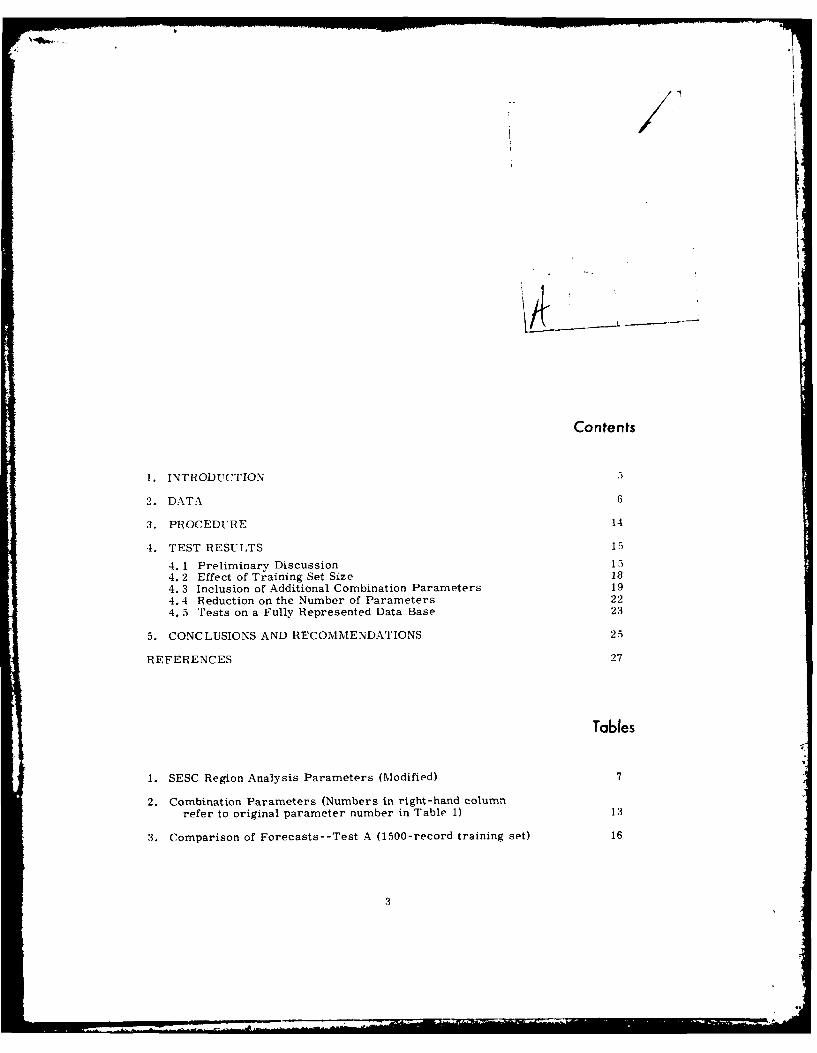
Contents
1. INTRODUCTION 5
2. DATA 6
3. PROCEDURE 14
4. TEST RESULTS 15
4. 1 Preliminary Discussion 154.2 Effect of Training Set Size 184.3 Inclusion of Additional Combination Parameters 194.4 Reduction on the Number of Parameters 224. 5 Tests on a Fully Represented Data Base 23
5. CONCLUSIONS AND RECOMMENDATIONS 25
REFERENCES 27
Tables
1. SESC Region Analysis Parameters (Modified) 7
2. Combination Parameters (Numbers in right-hand columnrefer to original parameter number in Table 1) 13
3. Comparison of Forecasts--Test A (1500-record training set) 16
3
Tables contd)
4. Parameters Submitted to Analysis and TheirFrequency of Selection in 19 Subsets--Test A 17
5. Comparison of Forecast Scores--Test A 17
6. Comparison of Scores Using 750-Record and 2095-Record Training Sets--Tests B and C 19
7. Additional Combination Parameters (Numbers in right-hand column refer to original parameter numbers inTable 1) 20
8. Parameters Submitted to Analysis and Their Frequencyof Selection in 19 Subsets--Tests 1), E, F, G and 11 21
9. Effects of Reduction in the Number of Input Parameters 22
10. Comparison of Forecasts Using a Pullv Represented I)ataBase--Test I (1500-record training set) 24
1I. Parameters Submlitted to Analysis and Their Frequtncyof Selection in 9 suh, Ots--Test 1 2-
12. t'omparison of Forecast Scores--Test 1 2-
4g
t.
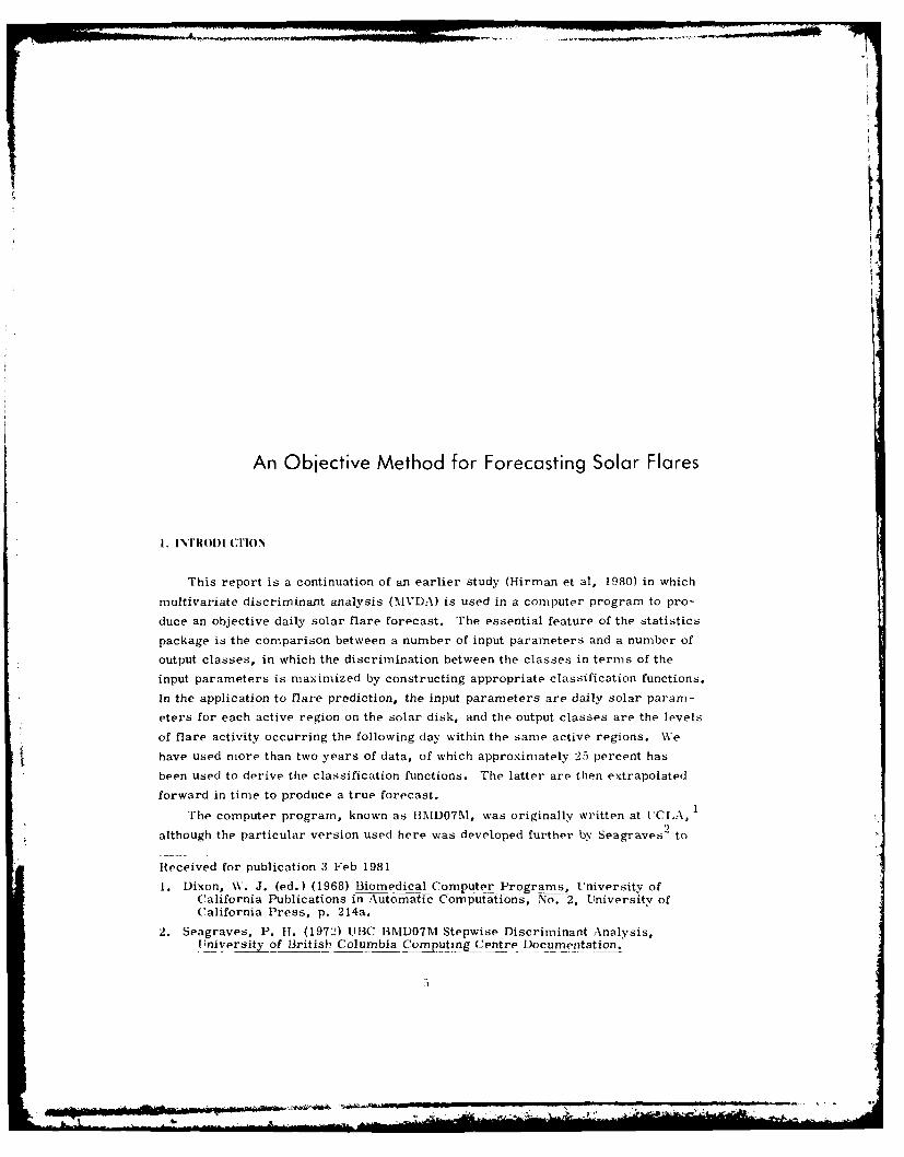
An Objective Method for Forecasting Solar Flares
I. I N"RO1)I (lON
This report is a continuation of an earlier study (Hirman et al, 1980) in which
multivariate discrirninant analysis (MVDA) is used in a computer program to pro-
duce an objective daily solar flare forecast. The essential feature of the statistics
package is the comparison between a number of input parameters and a number of
output classes, in which the discrimination between the classes in terms of the
input parameters is maximized by constructing appropriate classification functions.
In the application to flare prediction, the input parameters are daily solar param-
eters for each active region on the solar disk, and the output classes are the levels
of flare activity occurring the following day within the same active regions. We
have used more than two years of data, of which approximately 25 percent has
been used to derive the classification functions. The latter are then extrapolated
forward in time to produce a true forecast.1
The computer program, known as BIMD07M, was originally written at UCLA,
although the particular version used here was developed further by Seagraves to
Heceived for publication 3 Feb 1981
1. Dixon, W. J. (ed.) (1968) Biomedical Computer Programs, University ofCalifornia Publications in Automatic Computations, No. 2, University ofCalifornia Press, p. 214a.
2. Seagraves, P. I. (1972) UBC BNID07M Stepwise Discriminant Analysis,University of British Columbia Computin C _entr i)ocumentation.

Include the CooloY aInd 1.ohno' clasificationl proce-dure, and VhC. I.:e henhruch
\ -I' techiu'ue. 'I'lhe ( oley, and I ohne,- PPIOdure iiop, alo Ia;euni forlm it.\
of variance0, .11,l this someltimes.- result- inl hotter ci,.- .- ifi.tio:i acoi'e, FliP
computational bur-den, hower' is increased !Ill(".~ re 1 slicltion
funct ions are not pi' sible: in-stead, canonical v-arial,, tijtd from the
orilinal input par~imeiters, 'iref ia~od as a rnfomto t ie~cthe r ti
dimnnlsion inl the olai~jficat ion formulas. :a .wIaclhefibrufch toch n:iiue eox
bias whenl the rf a casfe its own daItahs.
Icomlplete- description of the riatheiiiatics is bevond the -copfe tf thlis- 1r01)11
I'lhe readel r'av Consult \11II11 nd 3-o1ad BaO" for refei-itc on i 1scrIiniiin it
analv -sis. A\ *iSCUSSIOn of the suitability Of ap~plyling various sfnst alrothods to
discrete input variables is cont ainod in \ecchia Pt al. 7 , ih latter point is of
nai'ticiilar in1to res1t bWecause the work of \ ecchiia et al uses the sanne iscrete da:tai
b)ase as usedu he-rein, to produce sotar flare prchahilitvy forecasts us iny di scrimin -
ant anal%-si, I without the ('(oil-\. and I ohnes procedure) iand locistic recression
An irmoo ftant feat nrcP of The Present st udv is the, comnpa rison oi the, ohliective,
COMPnteOr telPcalst with a1 SUhjectiVe, conve%-ntional forecast Mopared durinLe thre
samne test tieriod for the samle active regyions on the sun. %%\ ithout such a henoh -
nmark fir relative evaiuation, the presentation of anv forecast method has con-
roc a~' duced merfit.
The data tised her'ein were obtained from the region Analysis pro gram at the
i'WAA Space Environment Services Center (SESC) in Boulder, Colorado. Th e
region analysis program collects daily a variety of solar parameters for each
active region on the solar disk. It is imnportant to note that there is no attempt
3. Cooley, \.\ ,and lohnes, P. R. (1962) \lultivariate Proce-dures for theBlehavioral Science-s, Wiley, New York.
4. Lachenbruch, P. A., and NMickey, M. 13. (1968) Technonletrics, 10: 1.
ai. Anderson, T. W. (19.58) An lntroduction to_ 1lultivariate StatisticalAnalysis,Wiley, New York.___
6. Rlao, C. R. (1974) Advanced Statistical Methods in Biometric Research,llafner.
7. Vecchia, D. F., Caldwell, G. A. , Tryon, P. V., and Jones, R3. H. (1980)in So1. -Terres. Pred. Proc. , Vol. :3, R. F. Donnelly (ed.) C -76.
RV.........
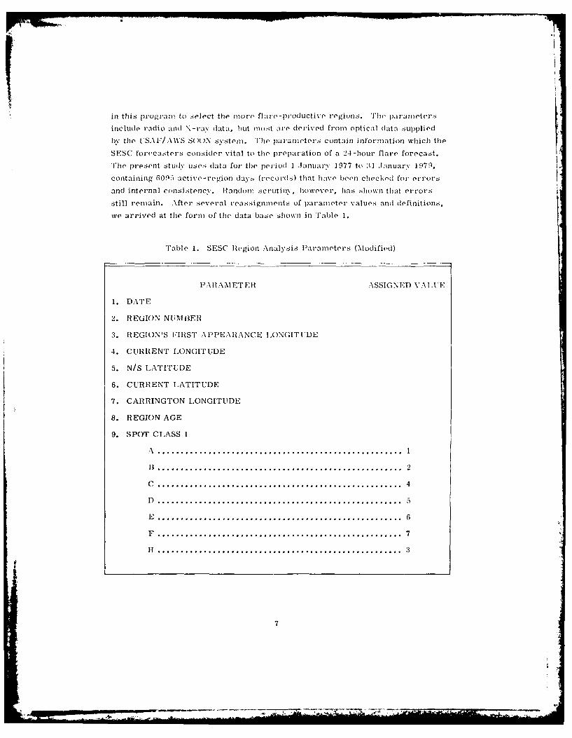
I1pPT-in this program to select the more flare -productive regions. The parameters
include radio and .\- ray dat a, hut most arie derived from opti cal dat a supplied
by the USA F/AWS SOO)N sys6tem. T'he parameters- contain information which the
SESC forecasters consider vital to the preparation of a 2-4-hour flare forecast,
The present studyN uses data for the period 1 lanuar.v 1977 to :31 Jainuary% 1979,
containing 6095 active-region days (records) that have been checked for errors
and internal consistencY. Handom scrutiny, however, has shown that errors
still remain. After several reassignments of parameter values and definitions,
we arrived at the form of the data base shown in Tbe1.
Table 1. SESC Region Analysis Parameters (Modified)
PARAMETER A\SSIGNED VALUE
1. DATE
2. REGION NUMHER
3. REGION'S FIRST APPEARANCE LO)NGITUDEi
4. CURRENT LONGITUDE
5. N/S LATITUDE
6. CURRENT LATITUDE
7. CAR RINGTON LONGITUDE
8. REGION AGE
9. SPOT CLASS 1
A........................................................ 1
i....................................................... 2
C....................................................... 4
D........................................................5
E........................................................ 6F .. ... .... ... ... .... ... .... ... ... .... ... ..
F........................................................73
7
-Lin =- --

I ahde 1. SF.U' kogion Analyi 'riramieters (Th'di fied) (continued)
10. SPOTl CLASS 2
r/ \ . . . . . . . . . . . . . . . . . . . . . . ... .1
S ...... .............................................. .
a . . . . . . . . . . . . . . . . . . . . . . . . . . . 3
........................................................ 4
k . . . . . . . . . . . . . . . . . . . . . . . . . ..
11. SPOT CLASS 3
X . ... ... ... ... ... ... ... ... ... ... ... .. ..
o........................................................ 2
12. MAGNETIC CLASS
N spots ... . . . . . . . . . . . . . . . . . . . ..0
Alphia .. . . . . . . . . . . . .. . . . . . . . . . .
Beta........................ ............................ 2
Beta-Ganinia .. . . . . . . . . . .. . . . . . . . . . 3
Gammna .. . . . . . . . . . . . . . . . . . . . . . . 4
Beta-Delta ............................................. 5
Beta -Gammia -Delta ..................................... 6
Gammia-Delta .......................................... 7
1:3. IMAGNETIC POLARITY OF STRONGEST FIELD................ (4/)
14. MAGNETIC FIELD STRENGTH............................... (Gauss)
15. MAGNETIC GRADIENTS...................................... (Gamma/ki)
16. INTERACTION WITH ANOTHER REGION
None ....................... .... .................... 1...0
Spots of opposite polarity converge (from less
than two degrees apart) ................................ 1
17. SUNSPOT DYNAMICS
No spots or no motion ................................... 0
Coalescing of spots ..................................... 1

Table 1. SESC' Region Analysis lParameter.- (Mlodified) (continued)
Spot rot atiot
Eelative motion between oppositel-, poled spots......
18. STAGE OF DEPVEIAPMEN'I
\0 spots ... . . . . . . . . . . . . . . . . . . . ..0
Maturt, group (stable)....................................1I
Decaying............................................... .I
Growing....................... ......................
Rapid decaly (spot numbers/ areas decrease b 50"........ 4
Rapid growth (spot numbers/areas increase by >50") .. 5
Rlapidi grow-th (, 100"').................................... 1)
19. LEADER/TRAILER FIEI.DS
Structure not definite.................................... 0
Returning Region........................................ 1
<5 dePg of neutral line and out of phase.....................-2
>5 deg of neutral line and in leader fields.................. 3
>5 deg of neutral line and in trailer fields.................. 4
*<.) deg of neutral line and in-phase....................... ..
20. RiETURNING REGION
21. SECTOR BOU1.NDARY RIELATIONSHIIP
22. ASSOCIATED FILAMNENT
None.................................................... 0
Filament unchanged.....................................I
Filament growving........................................ 2
Filament disappeared within past 24 hirs................... :
Fila-ment darkens or is active............................ 4
23. EMBEDDED FILAMENT
Non e................................................... 0
Filament present.......................................I
Active filament..........................................-2
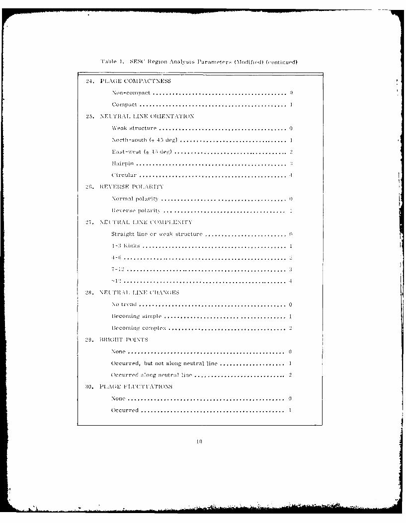
Table 1. SESC Region Analysis Parameters (Modifiod) (continued)
24. PLAGE COMPACTNIESS
Non-com pact ......................................... 0
Com pact .............................................
25. NEITrHAI, LINE OIIIENTATION
W eak structure ....................................... 0
North-south (± 45 deg) ................................. 1
East-west (± 45 deg) ................................... 2
IIairpin .......................................... . 3
Circular ................................................
26. IxEVESE POTAITY
Normal polarity. ........................................ 0
Ieverse polarity......................................... 1
27. NEI TIHAL LINE C(O13I ,E'NITY
Straight line or weak structure ...........................
1-S K inks ............................................ I
- .................................................. 2
712 .....................................................
~1.................................................... 4
28. NEt TlAI. LINE ('11:\NGES
No tren..d ............................................. 0
Becoming simple ..................................... I
lBecomini complex .................................... 2
29. IIIIGIT I'(IN'TS
None ................................................ 0
Occurred, but not along neutral line .................... I
)ccurred along neutral line ............................ 2
30. PIAGE FLUCTUATIONS
None ................................................ 0
Occurred ............................................ 1
10

Table 1. SESC Region Analysis Parameters (Modified) (continued)
31. ISOLATED POLE
32. EMERGING FLUX
None, or region is new ................................ 0
New flux emerges within spot group ...................... 1
New flux emerges near region (within 5 deg) ............. 2
33. ARCH FILAMENT SYSTEM
34. RADIO BURST/SWEEP
None occurred .......................................... 0
>250 flux units at 10 cm ............................... I
>1000 flux units at 10 cm .............................. 2
Type III ............................................. 3
Type IV................................................. 4
Type II and I%. ......................................... 5
V Burst ............................................. 6
Major/complex 10 cm burst .............................. 7
-1000 flux units at 10 cm plus a U burst, or
Type III and IV, or
250 flux units at 10 cm plus Type III and IN ............ 8
35. REGION'S FIRST APPEARANCE (TRANSIT HISTORY)
36. FLARE HISTORY
No flares have occurred ................................ 0
C class flares have occurred ........................... I
M class flares have occurred .......................... 2
X class flares have occurred ............................ 3
37. FLARES TODAY
None .................................................. 0
C class .... ....... ................................. 1
M class ................................................ 2
X class ............................. ................. 3
11
4
j - - -- ,.,.,
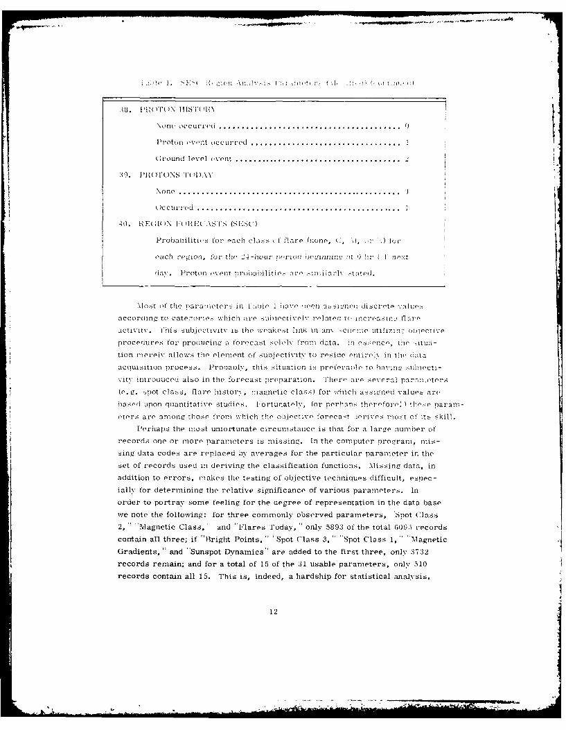
Proton e e toccurred .................................
\one ...cc . . .. .. .. . .. .. . .. .. .. . .. .. .
Ocrrend .e.l.v........................................
4o. It ECLI IN I:(1131.(.\SFS (SILSC)
I-rohabilities6 for each class .I flare (none, Ci, 1, .r \) for
each region, z .oi the 24-hour pen on otiinL'~t 0 hir I next
dayv. Proton ev-ent probahilIitie .a re .sn1 a rlv -t ated.
.%lost of the parameoters in 1 :,oie I hiave ueen a, signen discrete- valurs
accoraing to cateoos x hich are( subirctivelv re-lated to, increasing flar
activity-. i'his subjectivity is the woake.5 t link in an% sceeUt ii7in'_ )!!eci 1:0
procedures for prociucin-, a forecast soeyfromn data. in es .-iencf, the- .itua -
tion m~ereiy allows the elennt of subjectivity to reside entirely in the data
acquisition process. 1Pronaulv, this situation is pera]eto haviney suhiecti-
vjitv introniuced also in the forecast preparation. There- are eea paranmeters
Ic .spot class, flare history, miagnetic class) for xhich assicrnod values are
tnaSed Upon quantitative, studies. Fortunately,, (or perhiaps therefore: th p ararr-
eters are amiona those from- which the oblective forecast! .(erives m-ost of its skill.
Peorhaps thle most unfortunate circum stance is that for a arenumber of
records one or miore, parameters is missing!. In the computer programi, mis-
sing data codes arE, replaced by averages for the particular parameter in the
set of records used in deriving the classification functions. Missing data, in
addition to errors, makes thle testing of objective techniques difficult, espec-
iallv for determining the relative significance of various parameters. In
order to portray some feeling for the degree of representation in the data base
we note the following: for three commonly observed paramieters, 'Spot Class
2, ' Magnetic Class, ''and "Flares Today, " only 5893 of the total 609.5 records
contain all three; if "Bright Points, " "Spot Class 3, " ''Spot Class 1, '''Magnetic
Gradients, " and ''Sunspot Dynamics" are added to the first three, only 3732
records remain; and for a total of 15 of the 31 usable parameters, only L510
records contain all 15. This is, indeed, a hardship for statistical analysis.
12

Nevertheless, we are able to show later that at least some of those frequently
missing parameters contain valuable predictive information.
The data base contains daily, region-by-region entries for the actual flare
activity, in addition to the official SSC subjectively derived flare forecast.
Thus, the information required for objective forecast testing, as well as for
comparison with the SESC forecast, is contained in the same base. Flares are
listed according to their peak soft (1-8 ) N-ray flux at I AI:- 5
(lass C: 10 - F < 10 watt m -
Class M: 10' 5 E < 10 4 watt m -
Class X: 10 4 < L watt m -
From the standpoint of geophysical environment studies, the classes M and X
are of greatest importance.
In addition to Table 1, six combination parameters (Table 2), derived from
certain original parameters, were included as input parameters. These six were
Table 2. Combination Parameters (Numbers in right-handcolumn refer to original parameter number in Table 1)
New Parameter No. Parameter Formula
1 9.10.11
2 9.10.11" 12
:3 9-10.11.32
4 14. 15. (17+25)
5 12.17.27
6 17. (25+27+28)
found to have possible predictive significance in the earlier study where twenty
such combination parameters were tested. 8 The derivation of combination param-
eters is based on intuitions about the form in which predictive information might
be contained in the data, and about physical quantities (e. g., energy stored in
sheared magnetic fields) presumed relatable to flares. The subject of these and
other combination parameters will be discussed in a later section.
8. Hirman, J. W., Neidig, D. F., Seagraves, P. H., Flowers, W. E., andWiborg, P. H. (1980) in Sol. -Terrest. Pred. Proc., Vol. 3, R. F. Donnelly(ed.), C-64.
13
AIL
3. fRRI llt RE
The region analysis parameters for today are independent of any informationon flakre 1ctiVitY Occurring tomiorrow; therefore, they can be used in practice,
today, to produce a flare forecast for tomorrow, assuming that predictive inforrma-
tion is present in the parameters. \We have used the first N records (with N = 1500,
as described below) as a 'training set" in order to derive the classification func-
tions for throe possible outcomes: 'No Iiare, . Flare, " and "' or \ Flare.
Al and N fln're: were grouped together as a single class in order to roduce, statisti-
cal noise caused by the relatively few cases of larger flares, The, classification
functions were then applied to new records, using only the input paranleter,, in
(,rder to produce a true forecast. The latter procedure was accomplishod in
steps of 2.50 records each, w%'ith the training set slidir ' ,v.rward in time-, 2,a()
records (approximately one month) after each stop. Thus, 'nr a 1510-rocord
training set, the remaining' 4,95-record test set requir, 1!! individual suietost.,
of 250 records each (except for the nineteenth). This slidin- bae techni(uo r ain-
tains a constant N records in the trainin' set, thereby assuring that the orocran .
is trained on recent data relative to the test subset. This, cornblined ,vith the
relatively small size of the to.st subset, minimizes the ,ffects of secular trend.,,
either of observational or solar origin, which migLht he pre.sent in the data.
"'Y, computer pI'o2'rao was trainoed on the N-ray class of the largest event(No Flare, C I"laro, or N1 F N .lare) occurring in the region in the 24-hour
period following the acquisition date of the input parameters. Thus, the computer
forecast is expressed in term. of probabIlities for the largest event to be in ono
of these classes. ''ho outcomes are mutually exclusive, with the sum of probabili-
ties over all classes equal to unity. The SESC forecast, however, is a probability
forecast for the occurrence of each class of event; i. e., a non-exclusive format..
In order to assess the quality of the computer forecast, we derived a comparison
forecast in the "exclusive" format by selecting the largest event class in the
SESC forecast that was assigned a probability greater than or equal to 0.5. Al-
though this is not an SESC forecast, it is probably representative of what would
be extant if the SESC chose to cast their predictions in this mode.
In the following test results we present the forecasts according to both the
standard multivariate discriminant analysis (MVDA) and the Cooley and Lohnes
procedure (MVDA/CL). There are important differences in the character of
these two forecasts, which, as will be shown later, may be used to advantage.
14
a=
a

t. TIEST RESI ITS
t.1I Preliianrml Iisrussuin
pV a re concerned mnainly with the behavior of thel cuinput or forecasts rela -
tive to the comparison forecast when, for example, changes are, made Ini thel
S170 of the t raining set, ChoiCe Of input paramernters, sol ar activity lee .i nd!
pe eCerit of missing dat a. In all cases we present the coimpute r forc ast i ung
with thel Comipari son forecast for thel iame set of test recorli. s<l s o included is
aI list of input parameters submiitted to analysis, alng with their. Ireiurencv of
selection inl clal sifvinj thle thllee( outcomes. Note, hlowever, that (fr, tto the 251)-
record increme;(nt tlhe nraingI1 sets alro Independrent of each other oni. w01h.11 >pa-
rated h% I rx ci ore -rhes
V i frs;t tep, %%, eliminaited I I parameters which weore not selected Ii i n'
or thel 1' ln e: l . l% Iig this, the procram was run again11 u~ilnr the remnIII-
Ing 21) Input I'lmtel.Th results are given in lablu., :i, -4, anda 5. '[h 1is
test VwIll -erveO A,~ an example foi- the dipa. used illu h i~thv rl;urt.
lahie0 ), Io%\ thel aIctual IlIntrix of region-day~ foroczl1- V. I" a*.1-l;rI\
:roevents, for thel three,( forecasts. l':ihlf 5, derived Irum, the, OAi Ii l'alo
~, Itl!)!M 1e- - the ll Iowingl:
F Poecent of forecasts; correct Ii the given -vent cil as
T Percent of region -day l argest events which weore forec aste-d
C (Ii ma1,tologv (pe ic 'nt of thle total riurn 1her of events, in thel Class)
t nweighted mloan of thel A's for. all three-event classes
\\ \\ ighfted mleain forec ast acc uracy (the sum of thel mlatrix
doenad o l erents i ivided I)\- the total number of forecasts,
,I, o'.olits, in all cass
Iff I I 'erc ent of fo recasts, thFat are one( matrix clemennt a waY' from
thel di alm id
1ff 2 T'001eit of foreca sts that a~re two matrix elements aiway fr'om
thel diag4onal
I he se variotis scores a r'e of inte rest because of the severial ways in which
ferec:i sts can he used. For exa inpie, thel F score, or percentage of forecasts
that a re correct, is the quait itv of inte rest to a custom er who cannot tolecrate
falIse ala tm s. A quLite- diffe rent requi reiment applies, however, Ii a situation
where surprise flares are unwelcome. Ini the latter case, the E score, is the
important mneasurr-rent. *tif course, knowinV the ctrstorner 's need Ii advance
allorws thel forecast to he bidased either toward tinderpredict ion, w.~hi ch tends to
improve thel F s;core, or toward overpredi ction, which Improves thel F score.
15
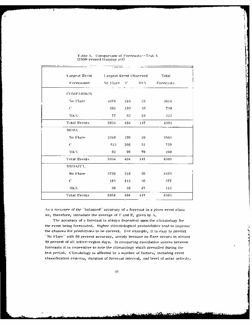
Table 3. Comparison of Forecasts--rest :%(1500-record training set)
largest Event Largest Event Observed Total
Forecasted No Flare C M4 x Forecasts
COMI' A ISON
No Flare 3376 213 25 3614
C 501 199 59 759
M&X 77 82 6:3 222
Total Events 3954 494 147 4595
MV1) A
No Flare 3349 190 26 3565
C 513 206 51 770
M&X 92 98 70 260
Total Events 3954 494 147 4595
MVD.A/C l
No Flare 3739 316 50 4105
C 185 142 50 377
M&N :30 36 47 113
Total Events 3954 494 147 4595
As a measure of the "balanced" accuracy of a forecast in a given event class
we, therefore, introduce the average of " and E, given by A.
The accuracy of a forecast is always dependent upon the climatology for
the event being forecasted. Higher climatological probabilities tend to improve
the chances for predictions to be correct. For example, it is easy to predict
''No Flare" with 90 percent accuracy, simply because no flare occurs in almost
90 percent of all active-region days. In comparing cumulative scores between
forecasts it is imperative to note the climatology which prevailed during the
test period. Climatology is affected by a number of factors, including event
classification criteria, duration of forecast interval, and level of solar activity.
In
I~
Table 4. Parameters Submitted to Analysis andTheir Frequency of Selection in 19 Subsets--Test A
Flares Today 19 New No. 1 9 Mag. Po!. 5
Bright Points 19 Mag. Grad. 9 Neut. L. Chg. 5
New No. 2 17 Mag. Class 6 Spot Class 3 4
Spot Dynam. 12 Hadio B/S 6 Spot (lass 2 3
New No. 5 12 Flare luist. 6 Spot Intpr.
Proton Hist. 11 Now No. 3 6 Emerg. Flux 1
Spot Class 1 9 New No. 4 6
Table 5. Comparison of Forecast Scores--Test .\
Forocastor Evnt F E A C I' (Iff 1 (Wff 2
CUMPkAIIlS(ON No Flare 93.4 85.4 89.4 86.1
C 26, 2 40.3 33.3 10.8 52.8 79.2 18.6 2.2
M&N 28. -1 42.9 35.6 3.2
\VDA No Flare 9:3.9 84.7 89.3 86.1
C 26.8 41.7 34.3 10.8 53.6 78.9 18.4 2.6
M&N 26.9 47.6 :37.3 :.2
MVD\/I, No Flare 91.1 94.6 92.8 86.1
C 37.7 28.7 33.2 10.8 54.3 85.5 12.8 1.7
Nl&X 41.6 :32.0 36.8 3.2
17

In essence, climatology is directly dependent upon "bin size. " Failure, to state
climatological conditions clearly (an unfortunately common practice) makes
intercomparison of forecasts almost impossible. 9It seems that this point can-
Blecause "'No Flare"' constitutes the majority of situations on thle sun, it comecs
as no surprise that solar flare forecasts are usually quite accurate overall; i.e.,
their weighted means (W) are high. It is of greater interest, however, to predict
flares than quiet conditions and, for this reason, the unweighted score U, given
simply by the mean of the A scores over all classes, has been included in Table 5.
Finally, we note that if a forecast is in error, it is better to be wrong by one
event class than by two. Thus, the tendency for the off-diagonal entries in the
matrix to cluster near the diagonal is an important measure when comparing fore-
cast scores which are similar otherwise. Table 5 includes a measure of this
error distribution in the form of the Off 1 and Off 2 scores.
The scores (F, E, and A) have uncertainties of approximately +1, +3, and
±5 for No Flare, C Flare, and M & X Flare, respectively. The V and W scores
have uncertainties of about ±l. Thus, in terms of A and U, the three forecasts
in Table 5 are essentially identical. The %1VDA/CL forecast definitely excels in
the W score, although this is mainly due to its tendency for underprediction, which
places a large number of forecasts in the No Flare column. The tendency for
underprediction in the MVDA/CL forecast is evident also in the F scores for C,
and M & X flares. being significantly higher than the corresponding E scores.
On the other hand, both the comparison and the MVDA forecast are biased toward
overprediction. Their overall similarity is quite striking.
4.2 Effect of Training Set Size
The number of records to be uced in the training set should be large enough
to provide sufficient statistics to train the computer program, yet small enough
to avoid the effects of trends in the data. The optimum number, while not known
from theory, may be determined empirically by varying the training set size and
comparing the scores of the resulting forecasts. Table 6 shows the results for
training sets of 750 and 2095 records. Together with Table 5 (1500-record train-
ing set) we find differences of only small significance. A close examination of
9. Simon, P., Smith, J. B., Ding, Y., Flowers, W., Guo, Q., Harvey,K. L., Hedeman, R., Martin, S. F., McKenna Lawlor, S., Lin, V.,Neidig, D., Obridko, V. N., Dodson Prince, H., Bust, D., Speich, D.,Starr, A., and Stepanyan, N. N. (1980) in Sol. -Terres. Pred. Proc.,Vol. 2, R. F. Donnelly (ed.) p. 287.
18
* .- ~..--~~--- -- f . . . *-- -. ~*~: -'. -
a -;I
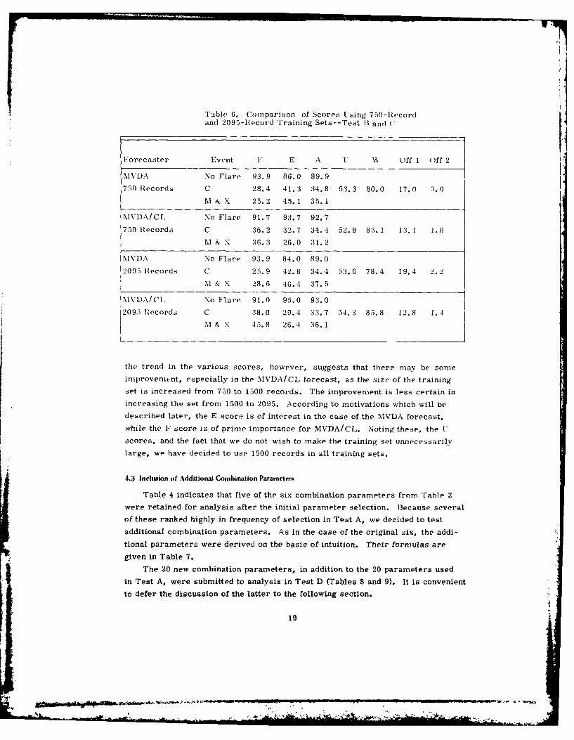
Table 6. Comparison of Scores Ising 750-Recordand 2095-Record Training Sets--Test 13 and '
Forecaster Event F E A U V uff I Off 2
MVDA No Flare 93.9 86.0 89.9
750 Records C 28.4 41.3 34.8 53.3 80.0 17.0 3.0
M & X 25.2 45.1 35.1
NIVD/CL No Flare 91.7 93.7 92.7
750 Records C 36.2 32.7 34.4 52.8 85.1 13.1 1.8
M & X 36.3 26.0 31.2
MVI)A No Flare 93.9 84.0 89.0
2095 Records C 25.9 42.8 34.4 53.6 78.4 19.4 2.2
& 28.6 46.4 37.5
MVDA/ICl. No Flare 91.0 95.0 93.0
2095 Records C 38.0 29.4 33.7 54.3 85.8 12.8 1.4
N I& X 45.8 26.4 36.1
the trend in the various scores, however, suggests that there may be some
improvenmnt, especially in the MVDA/CL forecast, as the size of the training
set is increased from 750 to 1500 records. The improvement is less certain in
increasing the set from 1500 to 2095. According to motivations which will be
described later, the E score is of interest in the case of the MVDA forecast,
while the F score is of prime importance for MVDA/CL. Noting these, the U
scores, and the fact that we do not wish to make the training set unnecessarily
large, we have decided to use 1500 records in all training sets.
4.3 Incltsion of Additional Combination Parameters
Table 4 indicates that five of the six combination parameters from Table 2
were retained for analysis after the initial parameter selection. Because several
of these ranked highly in frequency of selection in Test A, we decided to test
additional combination parameters. As in the case of the original six, the addi-
tional parameters were derived on the basis of intuition. Their formulas are
given in Table 7.
The 20 new combination parameters, in addition to the 20 parameters used
in Test A, were submitted to analysis in Test D (Tables 8 and 9). It is convenient
to defer the discussion of the latter to the following section.
19
was""*
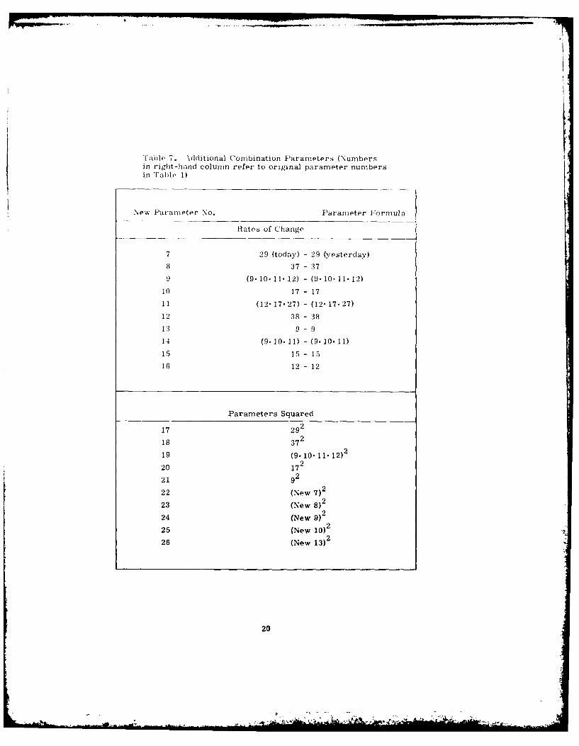
Table 7. Additional Combination Parameters (Numbersin right-hand column refer to original parameter numbersin "I'abhl 1)
New Parameter No. Parameter Formula
Rates of Change
7 29 (today) - 29 (yesterday)
8 37 - 37
(9 10. 11. 12) - (9.10.11-12)
10 17 - 17
11 (12" 17.27) - (12 17.27)
12 38 - '38
13 9 - 9
14 (9.10.11) - (9.10.11)
15 15- 15
16 12 - 12
Parameters Squared
17 292
18 372
19 (9.10.11.12)2
20 172
21 92
22 (New 7)2
23 (New 8)2
24 (New 9)2
25 (New 10)2
26 (New 13)2
20
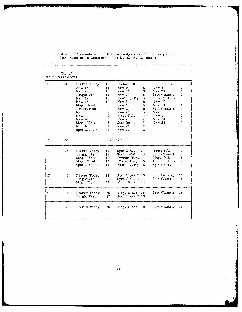
Table 8. Parameters Submitted to Analysis and Their Frequencyof Selection in 19 Subsets--Tests D, E, F, G, and I
No. ofTest Parameters
D 40 Flares Today 19 Radio B/S 6 Flare list. 2New 18 17 New 9 6 New 4 2New 2 16 New 12 6 New 23 2Bright Pts. 14 New 1 5 Spot Class 2 1New 19 12 Neut. L. Chg. 5 Emerg. Flux INew 15 10 New 5 5 New 17 1Mag. Grad. 9 New 14 5 New 19 1Proton I-list. 9 New 21 5 Spot Class 1 0New 3 9 New 22 5 New I 0New 8 9 Mag. Pol. 4 New 13 0New 20 8 New 7 4 New 16 0Mag. Class 7 Spot Inter. 3 New 26 0New 10 7 New 25 3Spot Class 3 6 New 20 2
A 20 See Table 4
E 15 Flares Today 19 Spot Class 3 14 Radio B/S 6Bright Pts. 19 Spot Dynam. 13 Spot Class 1 5Mag. Class 16 Proton Hist. 11 Mag. Pol. 5Mag. Grad. 16 Flare Hist. 10 Emerg. Flux 4Spot Class 2 14 Neut. L. Chg. 6 Spot Inter. 3
F 8 Flares Today 19 Spot Class 2 16 Spot Dynam. 11Bright Pts. 19 Spot Class 3 14 Spot Class 5Mag. Class 17 Mag. Grad. 13
G 5 Flares Today 19 Mlag. Class 18 Spot Class 3 15Bright Pts. 19 Spot Class 2 16
H 3 Flares Today 19 Mag. Class 19 Spot Class 2 19
21

Table 9. Effects of Reduction in the Number of Input Parameters
Forecaster Number ofParameters U W Off 1 Off 2 R
COMPARISON 52.8 79.2 18.6 2.2 2.22
TEST D MVDA 40 53.8 79.5 18.4 2.1 2.38MVDA/CL 54.6 85.1 13.4 1. 5 0.73
TEST A MVDA 20 53.6 78.9 18.4 2.6 2.63MVDA/CL 54.3 85.5 12.8 1.7 0.60
TEST E MVDA 15 52.4 78.1 18.7 3.2 2.80MVDA/CL 53.9 85.4 12.8 1.8 0.65
TEST F MVDA 8 52.2 78.0 18.6 3.4 2.83MVDA/CL 53.3 85.0 13.4 1.6 0.71
TEST G MVDA 5 53.0 77.6 18.5 3.9 3.02MVDA/CL 53.7 84.4 14.0 1.7 0.83
TEST H MVDA 3 51.5 78.2 17.5 4.3 2.72MVDA/CL 53.5 83. 2 13.3 1.5 0.61
4.4 Reduction in the Number of Parameters
The computer forecast was subjected to a series of reductions (Tests E, F,
G, and H) in the number of input parameters, according to Table 8, with the
corresponding forecast results summarized in Table 9. Table 9 displays the
effects of parameter reduction beginning with 40 parameters and ending with
only three. In addition to the previously used scores we introduce R, the ratio
of the number of matrix entries below the diagonal to tile number above the
diagonal. This ratio provides a measure of the asymmetry of the forecast, with
values greater than unity indicating overprediction, and values less than unity
indicating underprediction.
Table 9 clearly illustrates that the reduction in the number of parameters
has a small but unfavorable effect on the computer forecasts. We may regard
the tendencies for R to depart further from unity, for Off 2 to increase, and for
U to decline, as evidence for progressively worsening forecasts. These three
effects are most noticeable in the MVDA forecast, while the latter effect alone is
marginally evident in MVDA/CL.
22
The effects of the parameter reduction are offset by the increase in the
number of records containing all or most of the parameters submitted for anal-
vsis in the reduced sets. This improvement in representation occurs because
in the reduction steps we usually eliminated those parameters that were least
significant; i. e., those chosen least often in the subsets of the previous test;
and, !enerallv, the lower the significance of a parameter, the more often it is
missing from tile data base. It is concluded, therefore, that the decline in fore-
cast quality in Table i would have been more pronounced had all parameters
been present in all records. 'This proves that there is valuable predictive infor-
mation contained in at least some of tihe 'less significant' parameters. It is
emphasized that, perhaps to a large degree, the lower significance of these
Parameters is due only to their frequent absence from the data base.
A final word must be noted regarding the combination parameters. Table 8
indicates that a number of these new parameters have been selected by the com-
puter program as significant in classifying the outcomes. Due to the complex
intercorrelations among various parameters, however, in addition to possible
variance stabilization effects and other statistical phenomena, we do not fully
understand the true significance of these comuination parameters. Questions
such as this probably must await further testing on data bases containing fewer
missing parameters.
t.5 lests on .1 Full~ Represented I);ita Base
The most importnnt test of the computer forecast is achieved in the case
where all the parameters submitted to analysis are present in all records of the
data base. Such a test, using the full set of parameters, is impossible with the
presently available data. A test can oe made on a fully represented base, how-
ever, if, for example, only eight parameters are used, and we are willing to
accept a reduced base of 37:12 records, of which only 2232 remain in the test set.
Such a test (1) was performed, and the results are shown in Tables 10, 11, and 12.
Test I shows a dramatic improvement in the MVDA/Cl computer forecast
in all scores, while the MVDA and comparison forecasts show smaller improve-
ments. These improvements occur despite the somewhat lower flare climatology
that applies to this particular test set. The fact that tile comparison (subjec-
tive) forecast scores are higher indicates that the more complete observational
coverage during this sample of records somehow benefits the subjective methods
also.
Due to the reduced number of records, the errors associated with the Test I
scores are about 50 percent higher than those stated earlier. Nevertheless, there
now seems no question that the MVDA/CL forecast is superior to the others.
23
a4
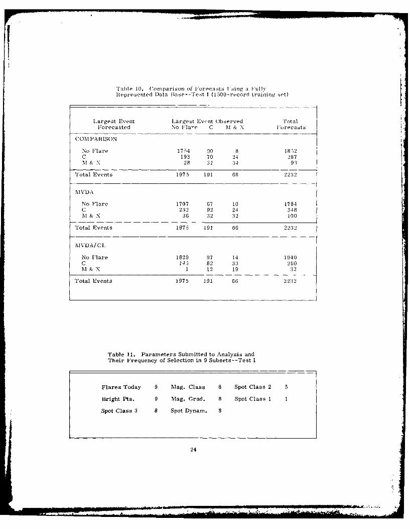
Table 10. Comparison of Forecasts Ising a FulvRepresented Data Base--Test I (1500-record training set)
Largest Event Largest Event Observed rotal
Forecasted No Flare C M & x Forecasts
COM PARISON
No Flare 1754 90 8 1852C 193 70 24 287M & X 28 31 :34 9:3
Total Events 1975 191 66 2232
MVDA
No Flare 1707 67 10 1784C 232 92 24 348M & X 36 32 32 100
Total Events 1975 191 66 2232
MVDA/CL
No Flare 1829 97 14 1940C 145 82 33 260M & X 1 12 19 32
Total Events 1975 191 66 2232
Table 11. Parameters Submitted to Analysis andTheir Frequency of Selection in 9 Subsets--Test I
Flares Today 9 Mag. Class 8 Spot Class 2 5
Bright Pts. 9 Mag. Grad. 8 Spot Class 1 1
Spot Class 3 8 Spot Dynam. 8
24
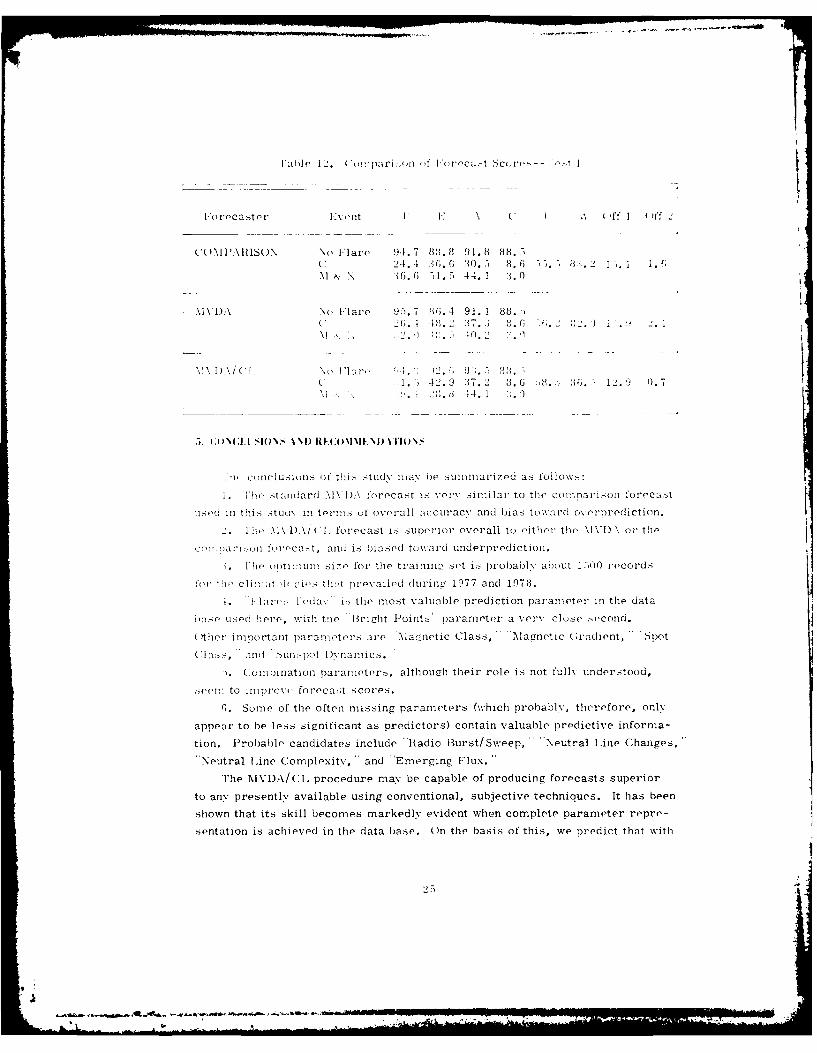
r-hoe 1.2. ('wtupari-.on (,' I-ooc-tScorxe--- 1'- 0, 1-
I -orocaster f-:"ont I F. A\ t*)ff I )f ul
C( )MIPAIISO-N \o Flare 94 .7 88. 8 9 1.H 88.L 24 4 -1 3 ; G. :0.4 8. . 8, .2 1 1.(N I & 26.( G51.5 44. 1 20
M\ I\tAN Flare 9 5. 7 H(6. 4 91.* 1 88.C 2(;. 4 4 . 3" . 8.- G
NIXl)\/C\ o Ilary.. : 2.5-12 .. 9 -;7. 2 8 .t 6 8.. 863. 12 .7
0i cunfllusioi) of thi, studY tn. 6e .-unimariz'ed a,, foilow :
Ihe -oandard Al\ D[A forecas-t is vertX similar to the coir-,narison 'or(,cai,;t
usned in t hi. 5 st11tAX In terms of ove-rall arC tracvy and bias tow,.ard overpreodjction.
Ml \ 1)\/ ('L forecast is supe-rior overall to either the Ml VDA) or the
201. artonforeca-t , and is biased toward underpredict ion.
I o t! iU umSi7e for the t rai ninc set i.s probhabl v ahout 1.500 records
for t'ho dl~i ate iens tha:t prevailed dulrind, 1977 and 1978.
i.4 1-1ares lda is the most valuablir prediction parameter in thet data
n''se tIS(( here," with ther 'Hlricht Points' parameter a verv close second.
ther important parameters are Alatinetic Class, AantcGdit, So
4.Comb1nation parameters, althougch their role is not full,-, understood,
sot: to iniprovo forecast scores.
6., Some of the often missing parameters (w.hich prohably, therefore, onl,,
appear to be less significant as predictors) contain valuable predictive informa-
tion. Probabler candidates include -Hadio Burst/Sweep, eurlLine Changes,
Neutral Line Complexity, ''and ''Energing Flux."
The NIVDA/Cl, procedure may be capable of producing forecasts superior
to any-, presently available using conventional, subjective techniques. It has been
shown that its skill becomes markedly evident when complete parameter repro-
spntation is achieved in the data base. Oin the basis of this, we predict that with
-4T
improvements in data consistency, as well as the inclusion of new, objective
parameters in the future, the computer forecast scores will continue to improve.
This study has led us to make the following recommendations concerning
the use of the two computer forecasts:
1. Provide a flare forecast derived from MVDA/CL for those customers
who cannot tolerate false flare alarms (note the comparison of F scores in
Table 12).
2. Provide a flare forecast derived from standard MVDA for those cus-
tomers who need to be forewarned of flares as often as possible (compare E
scores in Table 12).
3. Improve the coverage for the parameters in Table I that are deemed
"less significant' by virtue of their frequent absence in the data base.
4. Improve the objectivity and consistency of all parameters.
26

References
1. Dixon, 'Ao J. (od.) (1968) Biomedical Computer Proerams, I niverity ofalifornia Publications in Automatic Computations, No. 2, (niversity
of Alifornia i're-, p. 214a.
2. Soacraves, P. II. (1972) t l( 1MD07M Stepwise Discriminant Analysis,tnivorsity of tritish Columbia Computing Centre Documentation.
:. ('oolev, V,. *., and ILohnes, P. RI. (1962) Multivariate 'rocedures for the}Bpbavioral Sciences, \% ilo5, New York. - -
4. 1.achenbruch, P, \., and Mickey, \. H. (1968) Technometrics, 10:1.
.5. \nderson, T. \. (1955) \n Introduction to \Multivariate Statistical\nalysis, \%iley.
6. Hao, U. R. (1974) Advanced Statistical Methods in Bliometric Research,Hafner.
7. \ecchia, D. F. , F aldvoll, i. A. , Tr' on, 1'.\., and Jones, l. 1t.(1980) in Sol. -Torroest. 'red. Proc. , Vol. it 1'.1 Donnolyx(('d. ), C -7a(".
8. Hirman, J. k. , Nvidig, i) . , Seagravos, P. 11. , Flownrs, \\ . ,and WVibora, I'. Fl. (1980) in Sol. -Terrost. Prod. Proc. , Vol. 2,R. F. Donnelly (rd. ), C-64.
9. Simon, P. , Smith, J. B. , l)ing, Y. , Flowers, \\., Guo, Q. , llarvv,K. L., Iledeman, 11., Martin, S. F., Mcenna Lawlor, S., Iin, V.,Neidig, 1)., Obridko, V. N. , IDodsom, Prince, 11., Rust, 1). , Speich,D., Starr, A., and Stopanvan, N.N. (1980) in Sol. -Terrost. Pred.Proc. , Vol. 2, II. I. Donnelly (pd. ), p. 287.
2 7

IIDA.TE
ILMED