89251 23 AppE 4/4/07 1:11 PM Page 799 Appendix Bode Diagrams

799

As we have seen, the frequency response plot is a very important tool foranalyzing a circuit’s behavior. Up to this point, however, we have shownqualitative sketches of the frequency response without discussing how tocreate such diagrams. The most efficient method for generating and plot-ting the amplitude and phase data is to use a digital computer; we can relyon it to give us accurate numerical plots of and versus .However, in some situations, preliminary sketches using Bode diagramscan help ensure the intelligent use of the computer.

A Bode diagram, or plot, is a graphical technique that gives a feel forthe frequency response of a circuit. These diagrams are named in recogni-tion of the pioneering work done by H.W. Bode.1 They are most useful forcircuits in which the poles and zeros of are reasonably well separated.

Like the qualitative frequency response plots seen thus far, a Bodediagram consists of two separate plots: One shows how the amplitude of

varies with frequency, and the other shows how the phase angle of varies with frequency. In Bode diagrams, the plots are made onsemilog graph paper for greater accuracy in representing the wide rangeof frequency values. In both the amplitude and phase plots, the frequencyis plotted on the horizontal log scale, and the amplitude and phase angleare plotted on the linear vertical scale.

E.1 Real, First-Order Poles and ZerosTo simplify the development of Bode diagrams, we begin by consideringonly cases where all the poles and zeros of are real and first order.Later we will present cases with complex and repeated poles and zeros.For our purposes, having a specific expression for is helpful. Hencewe base the discussion on

(E.1)

from which

(E.2)

The first step in making Bode diagrams is to put the expression forin a standard form, which we derive simply by dividing out the

poles and zeros:

(E.3)H( jv) =

Kz1(1 + jv>z1)

p1( jv)(1 + jv>p1) .

H( jv)

H( jv) =

K( jv + z1)jv( jv + p1)

.

H(s) =

K(s + z1)s(s + p1)

,

H(s)

H(s)

H( jv)H( jv)

H(s)

vu( jv)|H( jv)|

Bode DiagramsEAppendix

1 See H. W. Bode, Network Analysis and Feedback Design (New York: Van Nostrand, 1945).

89251_23_AppE 4/4/07 1:11 PM Page 799

Electric Circuits, Eighth Edition, by James A. Nilsson and Susan A. Riedel.ISBN-13: 978-0-13-198922-1. © 2008 Pearson Education, Inc., Upper Saddle River, NJ. All rights reserved.

This material is protected by Copyright and written permission should be obtained from the publisher prior to any prohibited reproduction, storage in a retrieval system, or transmission in any form or by any means, electronic, mechanical, photocopying, recording, or likewise.

800 Bode Diagrams

Next we let represent the constant quantity , and at thesame time we express in polar form:

(E.4)

From Eq. E.4,

(E.5)

(E.6)

By definition, the phase angles and are

(E.7)

(E.8)

The Bode diagrams consist of plotting Eq. E.5 (amplitude) and Eq. E.6(phase) as functions of .

E.2 Straight-Line Amplitude PlotsThe amplitude plot involves the multiplication and division of factorsassociated with the poles and zeros of . We reduce this multiplicationand division to addition and subtraction by expressing the amplitude of

in terms of a logarithmic value: the decibel (dB).2 The amplitude of in decibels is

(E.9)

To give you a feel for the unit of decibels, Table E.1 provides a translationbetween the actual value of several amplitudes and their values in deci-bels. Expressing Eq. E.5 in terms of decibels gives

(E.10) - 20 log10 v - 20 log10|1 + jv>p1|.

= 20 log10 Ko + 20 log10|1 + jv>z1|

AdB = 20 log10 Ko|1 + jv>z1|

v|1 + jv>p1|

AdB = 20 log10|H( jv)|.

H( jv)H( jv)

H(s)

v

b1 = tan -1v>p1.

c1 = tan -1v>z1;

b1c1

u(v) = c1 - 90 �- b1.

|H( jv)| =

Ko|1 + jv>z1|

v|1 + jv>p1| ,

=

Ko|1 + jv>z1|

|v||1 + jv>p1| l(c1 - 90 �

- b1).

H( jv) =

Ko|1 + jv>z1| lc1

|v| l90 � |1 + jv>p1| lb1

H( jv)Kz1>p1Ko

2 See Appendix D for more information regarding the decibel.

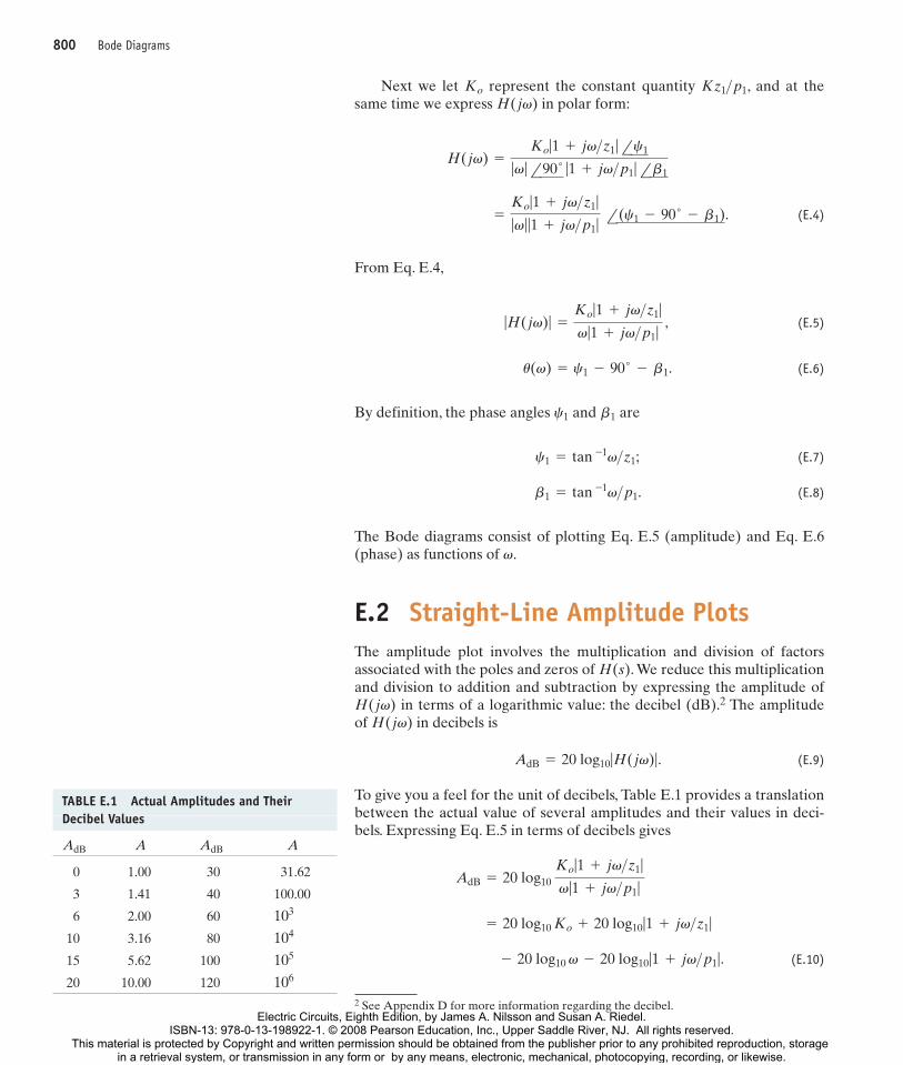
TABLE E.1 Actual Amplitudes and TheirDecibel Values

0 1.00 30 31.62

3 1.41 40 100.00

6 2.00 60

10 3.16 80

15 5.62 100

20 10.00 120 106

105

104

103

AAdBAAdB

89251_23_AppE 4/4/07 1:11 PM Page 800



E.2 Straight-Line Amplitude Plots 801

The key to plotting Eq. E.10 is to plot each term in the equation sepa-rately and then combine the separate plots graphically. The individual fac-tors are easy to plot because they can be approximated in all cases bystraight lines.

The plot of is a horizontal straight line because is not afunction of frequency. The value of this term is positive for , zerofor , and negative for .

Two straight lines approximate the plot of . For smallvalues of , the magnitude is approximately 1, and therefore

(E.11)

For large values of , the magnitude is approximately ,and therefore

(E.12)

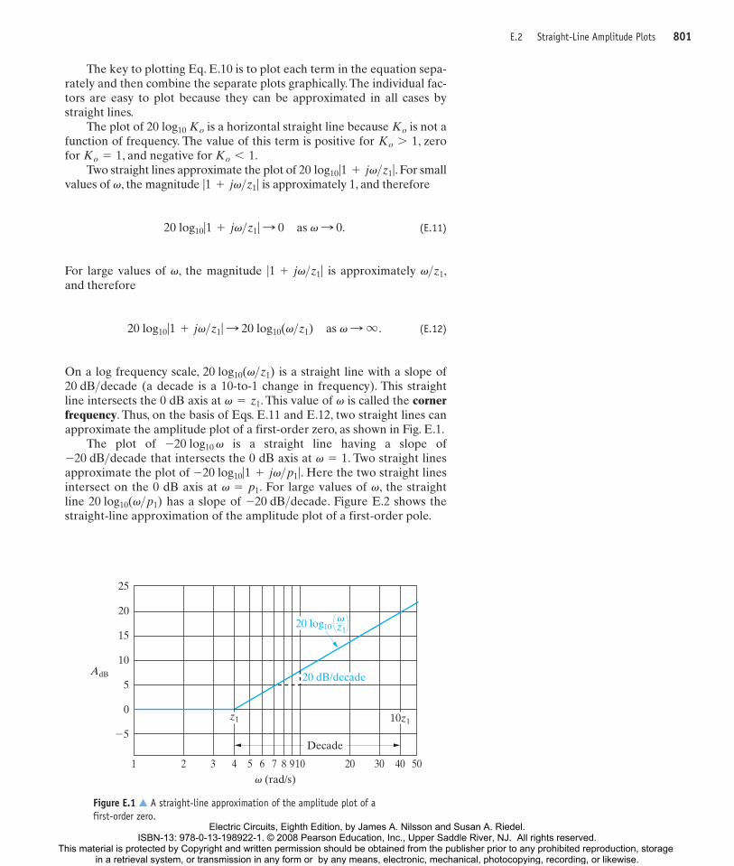
On a log frequency scale, is a straight line with a slope of(a decade is a 10-to-1 change in frequency). This straight

line intersects the 0 dB axis at . This value of is called the cornerfrequency. Thus, on the basis of Eqs. E.11 and E.12, two straight lines canapproximate the amplitude plot of a first-order zero, as shown in Fig. E.1.

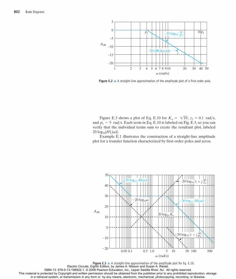
The plot of is a straight line having a slope ofthat intersects the 0 dB axis at . Two straight lines

approximate the plot of . Here the two straight linesintersect on the 0 dB axis at . For large values of , the straightline has a slope of . Figure E.2 shows thestraight-line approximation of the amplitude plot of a first-order pole.

-20 dB>decade20 log10(v>p1)vv = p1

-20 log10|1 + jv>p1|v = 1-20 dB>decade

-20 log10 v

vv = z1

20 dB>decade20 log10(v>z1)

20 log10|1 + jv>z1| : 20 log10(v>z1) as v: q .

v>z1|1 + jv>z1|v

20 log10|1 + jv>z1| : 0 as v: 0.

|1 + jv>z1|v

20 log10|1 + jv>z1|Ko 6 1Ko = 1

Ko 7 1Ko20 log10 Ko

�5

1 2 3 4 5 6 7v (rad/s)

8 910 20 30 40 50

0

5

10AdB

15

20

25

Decade

20 dB/decade

10z1z1

20 log10 z1v

Figure E.1 � A straight-line approximation of the amplitude plot of a first-order zero.

89251_23_AppE 4/4/07 1:11 PM Page 801



802 Bode Diagrams

20 log10 1 � j z1v

�20 log10 1 � j p1v

�20 log10v

10

5020 log10 |H(jv)|

20 log10 Ko

40

30

20AdB

0

�10

�200.05 0.1 0.5 1.0 5

v (rad/s)10 50 100 500

20 log10 |H(jv)|

Figure E.3 � A straight-line approximation of the amplitude plot for Eq. E.10.

Figure E.3 shows a plot of Eq. E.10 for ,and Each term in Eq. E.10 is labeled on Fig. E.3, so you canverify that the individual terms sum to create the resultant plot, labeled

.Example E.1 illustrates the construction of a straight-line amplitude

plot for a transfer function characterized by first-order poles and zeros.

20 log10|H( jv)|

p1 = 5 rad>s.z1 = 0.1 rad>s,Ko = 110

1 2 3 4 5 6 7 8v (rad/s)

910 20 30 40 50

–20

–15

–10

–5

0

5

AdB

p1 10p1–20 log10 p1v

–20 dB/decade

Figure E.2 � A straight-line approximation of the amplitude plot of a first-order pole.

89251_23_AppE 4/4/07 1:11 PM Page 802



E.2 Straight-Line Amplitude Plots 803

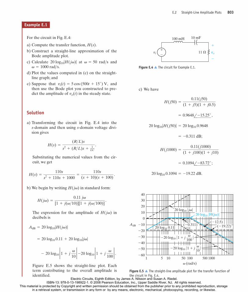
For the circuit in Fig. E.4:

a) Compute the transfer function, .

b) Construct a straight-line approximation of theBode amplitude plot.

c) Calculate at and

d) Plot the values computed in (c) on the straight-line graph; and

e) Suppose that andthen use the Bode plot you constructed to pre-dict the amplitude of in the steady state.

Solution

a) Transforming the circuit in Fig. E.4 into the s-domain and then using s-domain voltage divi-sion gives

Substituting the numerical values from the cir-cuit, we get

b) We begin by writing in standard form:

The expression for the amplitude of indecibels is

Figure E.5 shows the straight-line plot. Eachterm contributing to the overall amplitude isidentified.

- 20 log10 2 1 + j v

102 -20 log10 2 1 + j

v

1002 .

= 20 log10 0.11 + 20 log10|jv|

AdB = 20 log10|H( jv)|

H( jv)

H( jv) =

0.11 jv[1 + j(v>10)][1 + j(v>100)]

.

H( jv)

H(s) =

110s

s2+ 110s + 1000

=

110s

(s + 10)(s + 100) .

H(s) =

(R>L)s

s2+ (R>L)s +

1LC

.

vo(t)

vi(t) = 5 cos (500t + 15 �) V,

v = 1000 rad>s.v = 50 rad>s20 log10|H( jv)|

H(s)

c) We have

20 log10 0.1094 = -19.22 dB.

= 0.1094l -83.72 � ;

H( j1000) =

0.11( j1000)(1 + j100)(1 + j10)

= -0.311 dB;

20 log10|H( j50)| = 20 log10 0.9648

= 0.9648l -15.25 � ,

H( j50) =

0.11( j50)(1 + j5)(1 + j0.5)

11 �

100 mH

vi

�

�

vo

10 mF

�

�

Figure E.4 � The circuit for Example E.1.

Example E.1

AdB

�20

�10

�30

�40

�50

�60

0

10

20

30

40

1 10 100 1000500505v (rad/s)

(�12.5)(�0.311) (�19.22)20 log10 0.11

20 log10 � jv�20 log10 �H(jv)�

�20 log10 �1 � j �v

100

�20 log10 �1 � j �v10

Figure E.5 � The straight-line amplitude plot for the transfer function ofthe circuit in Fig. E.4.

89251_23_AppE 4/4/07 1:11 PM Page 803



804 Bode Diagrams

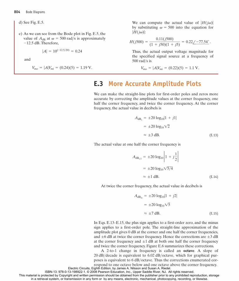
E.3 More Accurate Amplitude PlotsWe can make the straight-line plots for first-order poles and zeros moreaccurate by correcting the amplitude values at the corner frequency, onehalf the corner frequency, and twice the corner frequency. At the cornerfrequency, the actual value in decibels is

(E.13)

The actual value at one half the corner frequency is

(E.14)

At twice the corner frequency, the actual value in decibels is

(E.15)

In Eqs. E.13–E.15, the plus sign applies to a first-order zero, and the minussign applies to a first-order pole. The straight-line approximation of theamplitude plot gives 0 dB at the corner and one half the corner frequencies,and at twice the corner frequency. Hence the corrections are at the corner frequency and at both one half the corner frequencyand twice the corner frequency. Figure E.6 summarizes these corrections.

A 2-to-1 change in frequency is called an octave. A slope ofis equivalent to which for graphical pur-

poses is equivalent to Thus the corrections enumerated cor-respond to one octave below and one octave above the corner frequency.

6 dB>octave.6.02 dB>octave,20 dB>decade

;1 dB;3 dB;6 dB

L ;7 dB.

= ;20 log1015

AdB2c= ;20 log10|1 + j2|

L ;1 dB.

= ;20 log1015>4 AdBc>2 = ;20 log10 2 1 + j

122

L ;3 dB.

= ;20 log1012

AdBc= ;20 log10|1 + j1|

d) See Fig. E.5.

e) As we can see from the Bode plot in Fig. E.5, thevalue of at is approximately

. Therefore,

and

Vmo = |A|Vmi = (0.24)(5) = 1.19 V.

|A| = 10(-12.5>20)= 0.24

-12.5 dBv = 500 rad>sAdB

We can compute the actual value of by substituting into the equation for

:

Thus, the actual output voltage magnitude forthe specified signal source at a frequency of

is

Vmo = |A|Vmi = (0.22)(5) = 1.1 V.

500 rad>s

H( j500) =

0.11( j500)(1 + j50)(1 + j5)

= 0.22l -77.54 � .

|H( jv)|v = 500

|H( jv)|

89251_23_AppE 4/4/07 1:11 PM Page 804



E.4 Straight-Line Phase Angle Plots 805

If the poles and zeros of are well separated, inserting these correc-tions into the overall amplitude plot and achieving a reasonably accuratecurve is relatively easy. However, if the poles and zeros are close together,the overlapping corrections are difficult to evaluate, and you’re better offusing the straight-line plot as a first estimate of the amplitude characteristic.Then use a computer to refine the calculations in the frequency range ofinterest.

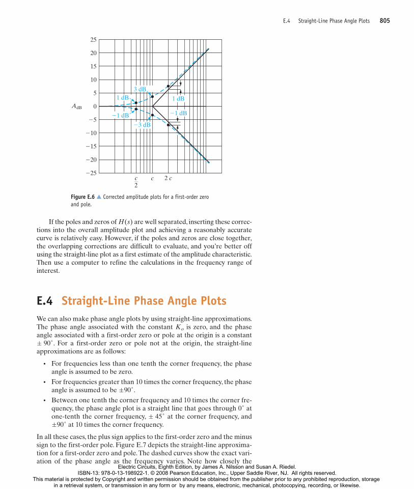
E.4 Straight-Line Phase Angle PlotsWe can also make phase angle plots by using straight-line approximations.The phase angle associated with the constant is zero, and the phaseangle associated with a first-order zero or pole at the origin is a constant

. For a first-order zero or pole not at the origin, the straight-lineapproximations are as follows:

• For frequencies less than one tenth the corner frequency, the phaseangle is assumed to be zero.

• For frequencies greater than 10 times the corner frequency, the phaseangle is assumed to be .

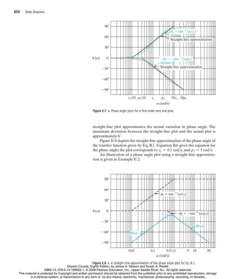
• Between one tenth the corner frequency and 10 times the corner fre-quency, the phase angle plot is a straight line that goes through atone-tenth the corner frequency, at the corner frequency, and

at 10 times the corner frequency.

In all these cases, the plus sign applies to the first-order zero and the minussign to the first-order pole. Figure E.7 depicts the straight-line approxima-tion for a first-order zero and pole.The dashed curves show the exact vari-ation of the phase angle as the frequency varies. Note how closely the

;90 �; 45 �

0 �

;90 �

; 90 �

Ko

H(s)

AdB

c2

c 2 c�25

�20

�15

�10

�5

10

15

20

25

0

5

�1 dB

1 dB1 dB3 dB

�1 dB

�3 dB

Figure E.6 � Corrected amplitude plots for a first-order zero and pole.

89251_23_AppE 4/4/07 1:11 PM Page 805



806 Bode Diagrams

straight-line plot approximates the actual variation in phase angle. Themaximum deviation between the straight-line plot and the actual plot isapproximately .

Figure E.8 depicts the straight-line approximation of the phase angle ofthe transfer function given by Eq. B.1. Equation B.6 gives the equation forthe phase angle; the plot corresponds to and

An illustration of a phase angle plot using a straight-line approxima-tion is given in Example E.2.

p1 = 5 rad>s.z1 = 0.1 rad>s,

6 �

30�

60�

90�

0

�30�

�60�

�90�

v (rad/s)

z1/10 p1/10 z1 p1 10z1 10p1

Straight-line approximation

u (v) �b1 � �tan�1 (v/p1)Actual

Straight-line approximation

c1 � tan�1 (v/z1)Actual

Figure E.7 � Phase angle plots for a first-order zero and pole.

90�

60�

30�

0

�30�

�60�

�90�

v (rad/s)0.01 0.1 0.5 5 10 501.0

u (v)

c1 � tan�1 (v/z1)

�b1 � �tan�1 (v/p1)

u(v)

u(v)

Figure E.8 � A straight-line approximation of the phase angle plot for Eq. B.1.

89251_23_AppE 4/4/07 1:11 PM Page 806



E.5 Bode Diagrams: Complex Poles and Zeros 807

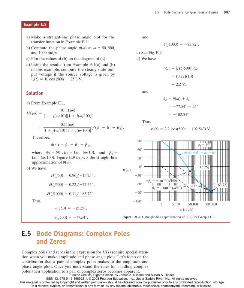
a) Make a straight-line phase angle plot for thetransfer function in Example E.1.

b) Compute the phase angle at and .

c) Plot the values of (b) on the diagram of (a).

d) Using the results from Example E.1(e) and (b)of this example, compute the steady-state out-put voltage if the source voltage is given by

Solution

a) From Example E.1,

vi(t) = 10 cos (500t - 25 �) V.

1000 rad>s v = 50, 500,u(v)

and

c) See Fig. E.9.

d) We have

and

Thus,

vo(t) = 2.2 cos(500t - 102.54 �) V.

= -102.54 � .

= -77.54 �- 25 �

uo = u(v) + ui

= 2.2 V,

= (0.22)(10)

Vmo = |H( j500)|Vmi

u( j1000) = -83.72 � .

Example E.2

�120�

�90�

�60�

�30�

0�

30�

60�

90�

1 10 100 1000500505

(�15.25)

(�77.54) (�83.72)

u (v)

c1 � 90�

u(v) � c1 � b1 � b2

�b2 � �tan�1 (v/100)

�b1 � �tan�1 (v/10)

v (rad/s)

Figure E.9 � A straight-line approximation of for Example E.2.u(v)

E.5 Bode Diagrams: Complex Poles and Zeros

Complex poles and zeros in the expression for require special atten-tion when you make amplitude and phase angle plots. Let’s focus on thecontribution that a pair of complex poles makes to the amplitude andphase angle plots. Once you understand the rules for handling complexpoles, their application to a pair of complex zeros becomes apparent.

H(s)

=

0.11|jv||1 + j(v>10)||1 + j(v>100)|

l(c1 - b1 - b2) .

H( jv) =

0.11( jv)[1 + j(v>10)][1 + j(v>100)]

Therefore,

where and Figure E.9 depicts the straight-line

approximation of .

b) We have

Thus,

u( j500) = -77.54 � ,

u( j50) = -15.25 � ,

H( j1000) = 0.11l -83.72 � .

H( j500) = 0.22l -77.54 � ,

H( j50) = 0.96l -15.25 � ,

u(v)tan-1(v>100).

b2 =c1 = 90 � , b1 = tan-1(v>10),

u(v) = c1 - b1 - b2,

89251_23_AppE 4/4/07 1:12 PM Page 807



808 Bode Diagrams

The complex poles and zeros of always appear in conjugatepairs. The first step in making either an amplitude or a phase angle plot ofa transfer function that contains complex poles is to combine the conju-gate pair into a single quadratic term. Thus, for

(E.16)

we first rewrite the product as

(E.17)

When making Bode diagrams, we write the quadratic term in a more con-venient form:

(E.18)

A direct comparison of the two forms shows that

(E.19)

and

(E.20)

The term is the corner frequency of the quadratic factor, and is thedamping coefficient of the quadratic term. The critical value of is 1. If

, the roots of the quadratic factor are complex, and we use Eq. E.18to represent the complex poles. If , we factor the quadratic factorinto and then plot amplitude and phase in accordancewith the discussion previously.Assuming that , we rewrite Eq. E.16 as

(E.21)

We then write Eq. E.21 in standard form by dividing through by the polesand zeros. For the quadratic term, we divide through by , so

(E.22)

from which

(E.23)

where

Before discussing the amplitude and phase angle diagrams associatedwith Eq. E.23, for convenience we replace the ratio by a new vari-able, u. Then

(E.24)

Now we write in polar form:

(E.25)H( jv) =

Ko

|(1 - u2) + j2zu|lb1 ,

H( jv)

H( jv) =

Ko

1 - u2+ j2zu

.

v>vn

Ko =

K

vn2 .

H( jv) =

Ko

1 - (v2>vn2) + j(2zv>vn)

,

H(s) =

K

vn2

1

1 + (s>vn)2+ 2z(s>vn)

,

vn

H(s) =

K

s2+ 2zvns + vn

2 .

z 6 1(s + p1)(s + p2)

z Ú 1z 6 1

z

zvn

zvn = a.

vn2

= a2+ b2

s2+ 2as + a2

+ b2= s2

+ 2zvns + vn2

.

(s + a)2+ b2

= s2+ 2as + a2

+ b2.

(s + a - jb)(s + a + jb)

H(s) =

K

(s + a - jb)(s + a + jb) ,

H(s)

89251_23_AppE 4/4/07 1:12 PM Page 808



E.6 Amplitude Plots 809

from which

(E.26)

and

(E.27)

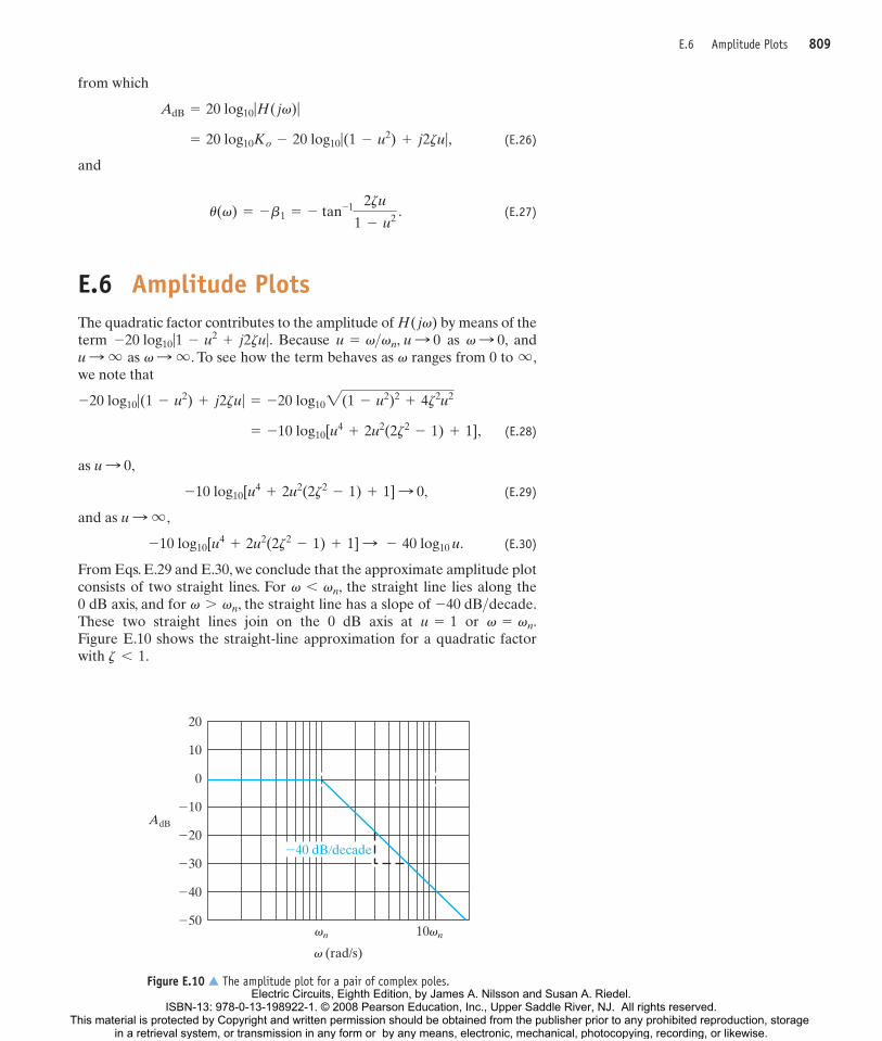
E.6 Amplitude PlotsThe quadratic factor contributes to the amplitude of by means of theterm . Because as , and

as . To see how the term behaves as ranges from 0 to ,we note that

(E.28)

as ,

(E.29)

and as ,

(E.30)

From Eqs. E.29 and E.30, we conclude that the approximate amplitude plotconsists of two straight lines. For , the straight line lies along the0 dB axis, and for , the straight line has a slope of .These two straight lines join on the 0 dB axis at or .Figure E.10 shows the straight-line approximation for a quadratic factorwith .z 6 1

v = vnu = 1-40 dB>decadev 7 vn

v 6 vn

-10 log10[u4

+ 2u2(2z2- 1) + 1] : - 40 log10 u.

u : q

-10 log10[u4

+ 2u2(2z2- 1) + 1] : 0,

u : 0

= -10 log10[u4

+ 2u2(2z2- 1) + 1],

-20 log10|(1 - u2) + j2zu| = -20 log102(1 - u2)2+ 4z2u2

qvv: qu : q

v: 0u = v>vn, u : 0-20 log10|1 - u2+ j2zu|

H( jv)

u(v) = -b1 = - tan-1 2zu

1 - u2 .

= 20 log10Ko - 20 log10|(1 - u2) + j2zu|,

AdB = 20 log10|H( jv)|

�50

�40

�30

�20

�10

20

0

10

�40 dB�decade

AdB

vn 10vn

v (rad/s)

Figure E.10 � The amplitude plot for a pair of complex poles.

89251_23_AppE 4/4/07 1:12 PM Page 809



810 Bode Diagrams

E.7 Correcting Straight-Line Amplitude Plots

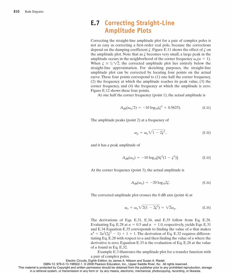
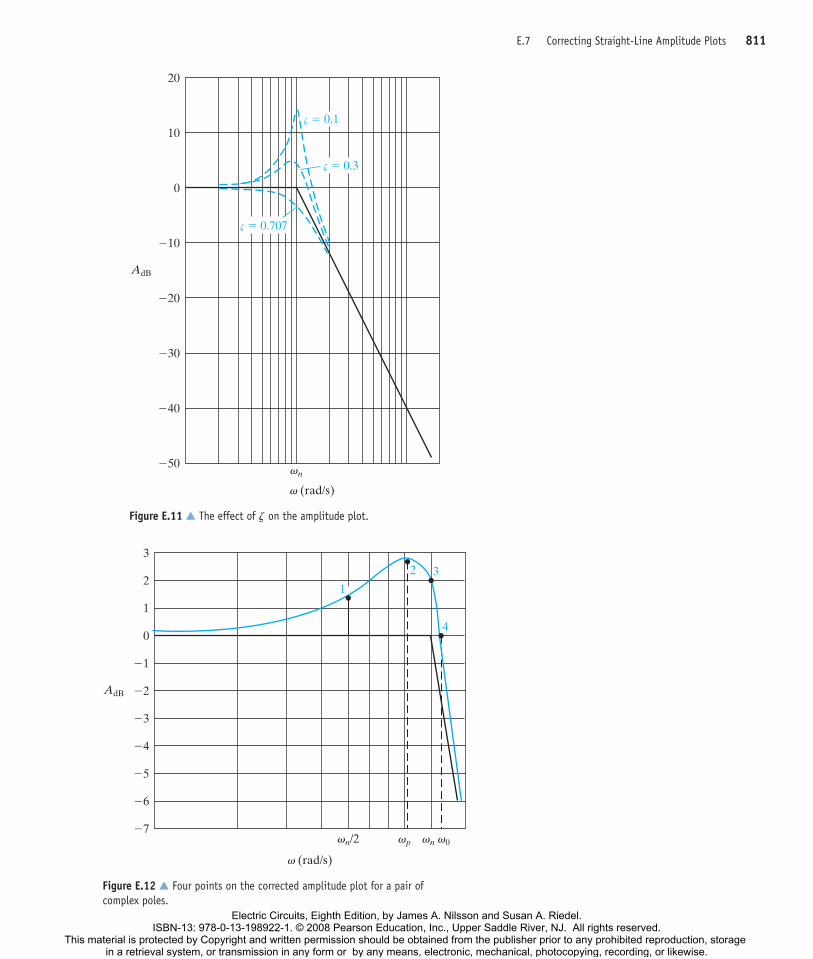
Correcting the straight-line amplitude plot for a pair of complex poles isnot as easy as correcting a first-order real pole, because the correctionsdepend on the damping coefficient . Figure E.11 shows the effect of onthe amplitude plot. Note that as becomes very small, a large peak in theamplitude occurs in the neighborhood of the corner frequency .When , the corrected amplitude plot lies entirely below thestraight-line approximation. For sketching purposes, the straight-lineamplitude plot can be corrected by locating four points on the actualcurve. These four points correspond to (1) one half the corner frequency,(2) the frequency at which the amplitude reaches its peak value, (3) thecorner frequency, and (4) the frequency at which the amplitude is zero.Figure E.12 shows these four points.

At one half the corner frequency (point 1), the actual amplitude is

(E.31)

The amplitude peaks (point 2) at a frequency of

(E.32)

and it has a peak amplitude of

(E.33)

At the corner frequency (point 3), the actual amplitude is

(E.34)

The corrected amplitude plot crosses the 0 dB axis (point 4) at

(E.35)

The derivations of Eqs. E.31, E.34, and E.35 follow from Eq. E.28.Evaluating Eq. E.28 at and , respectively, yields Eqs. E.31and E.34 Equation E.35 corresponds to finding the value of u that makes

. The derivation of Eq. E.32 requires differen-tiating Eq. E.28 with respect to u and then finding the value of u where thederivative is zero. Equation E.33 is the evaluation of Eq. E.28 at the valueof u found in Eq. E.32.

Example E.3 illustrates the amplitude plot for a transfer function witha pair of complex poles.

u4+ 2u2(2z2

- 1) + 1 = 1

u = 1.0u = 0.5

vo = vn22(1 - 2z2) = 12vp.

AdB(vn) = -20 log102z.

AdB(vp) = -10 log10[4z2(1 - z2)].

vp = vn21 - 2z2 ,

AdB(vn>2) = -10 log10(z2

+ 0.5625).

z Ú 1>12vn(u = 1)

z

zz

89251_23_AppE 4/4/07 1:12 PM Page 810



E.7 Correcting Straight-Line Amplitude Plots 811

�50

�40

�30

�10

0

10

20

�20

z � 0.707

z � 0.3

z � 0.1

vn

v (rad/s)

AdB

Figure E.11 � The effect of on the amplitude plot.z

1

2 3

4

�7

�6

�5

�4

�3

�2

�1

0

1

2

3

AdB

v (rad/s)

vn/2 vp vn v0

Figure E.12 � Four points on the corrected amplitude plot for a pair of complex poles.

89251_23_AppE 4/4/07 1:12 PM Page 811



812 Bode Diagrams

Compute the transfer function for the circuit shownin Fig. E.13.

a) What is the value of the corner frequency in radi-ans per second?

b) What is the value of ?

c) What is the value of the damping coefficient?

d) Make a straight-line amplitude plot ranging from10 to .

e) Calculate and sketch the actual amplitude indecibels at , , , and .

f) From the straight-line amplitude plot, describethe type of filter represented by the circuit inFig. E.13 and estimate its cutoff frequency, .vc

vovnvpvn>2500 rad>s

Ko

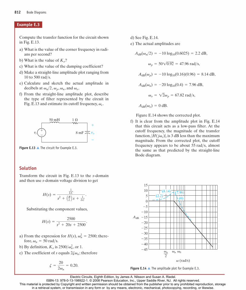
d) See Fig. E.14.

e) The actual amplitudes are

Figure E.14 shows the corrected plot.

f) It is clear from the amplitude plot in Fig. E.14that this circuit acts as a low-pass filter. At thecutoff frequency, the magnitude of the transferfunction, , is 3 dB less than the maximummagnitude. From the corrected plot, the cutofffrequency appears to be about almostthe same as that predicted by the straight-lineBode diagram.

55 rad>s,

|H( jvc)|

AdB(vo) = 0 dB.

vo = 12vp = 67.82 rad>s,

AdB(vn) = -20 log10(0.4) = 7.96 dB,

AdB(vp) = -10 log10(0.16)(0.96) = 8.14 dB,

vp = 5010.92 = 47.96 rad>s,

AdB(vn>2) = -10 log10(0.6025) = 2.2 dB,

50 mH 1 �

vi�

�vo

�

�

8 mF


(7.96)(8.14)

(0)

�40

�35

�30

�25

�20

�15

�10

�5

0

5 (2.2)10

�45

AdB

15

v (rad/s)

vn

2vn v0

Figure E.14 � The amplitude plot for Example E.3.

Example E.3

SolutionTransform the circuit in Fig. E.13 to the s-domainand then use s-domain voltage division to get

Substituting the component values,

a) From the expression for , ; there-fore,

b) By definition, is , or 1.

c) The coefficient of s equals ; therefore

z =

202vn

= 0.20.

2zvn

2500>vn2Ko

vn = 50 rad>s.vn

2= 2500H(s)

H(s) =

2500

s2+ 20s + 2500

.

H(s) =

1LC

s2+ ARL B s +

1LC

.

89251_23_AppE 4/4/07 1:12 PM Page 812



E.8 Phase Angle Plots 813

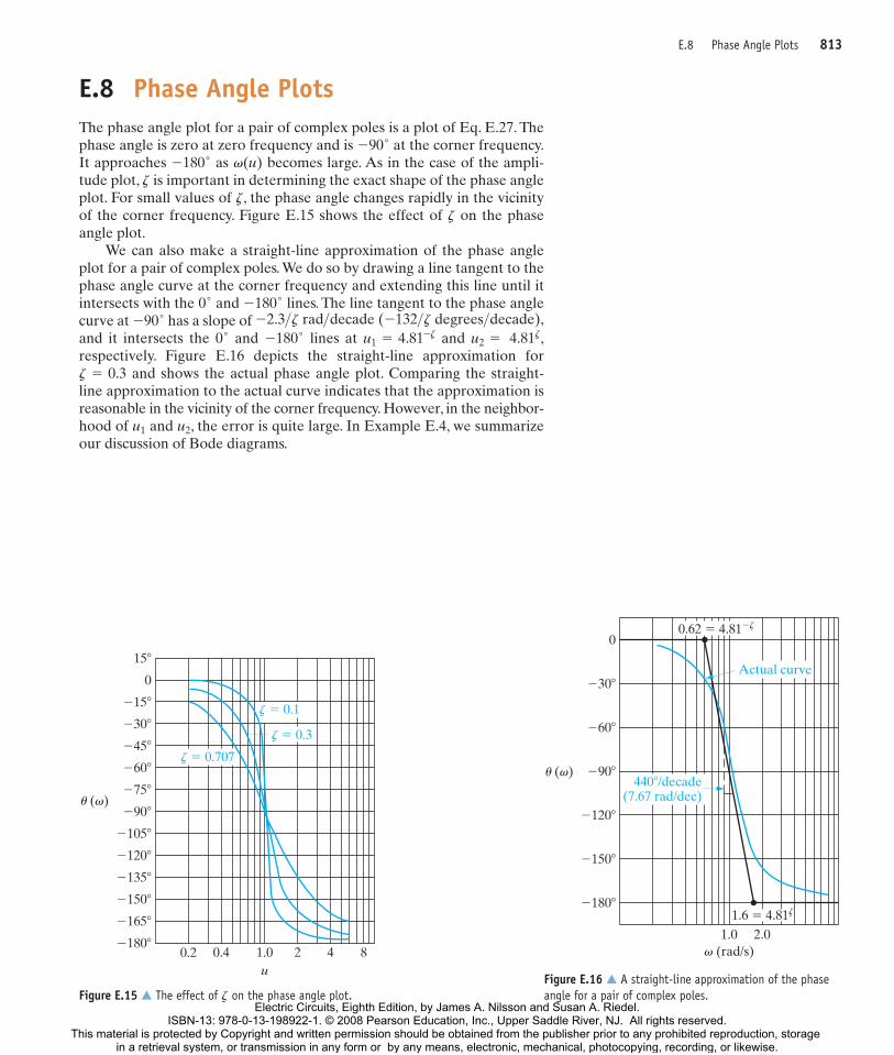
E.8 Phase Angle PlotsThe phase angle plot for a pair of complex poles is a plot of Eq. E.27. Thephase angle is zero at zero frequency and is at the corner frequency.It approaches as becomes large. As in the case of the ampli-tude plot, is important in determining the exact shape of the phase angleplot. For small values of , the phase angle changes rapidly in the vicinityof the corner frequency. Figure E.15 shows the effect of on the phaseangle plot.

We can also make a straight-line approximation of the phase angleplot for a pair of complex poles. We do so by drawing a line tangent to thephase angle curve at the corner frequency and extending this line until itintersects with the and lines. The line tangent to the phase anglecurve at has a slope of and it intersects the and lines at and ,respectively. Figure E.16 depicts the straight-line approximation for

and shows the actual phase angle plot. Comparing the straight-line approximation to the actual curve indicates that the approximation isreasonable in the vicinity of the corner frequency. However, in the neighbor-hood of and , the error is quite large. In Example E.4, we summarizeour discussion of Bode diagrams.

u2u1

z = 0.3

u2 = 4.81zu1 = 4.81-z-180 �0 �

-2.3>z rad>decade (-132>z degrees>decade),-90 �-180 �0 �

z

z

z

v(u)-180 �-90 �

z � 0.707

�180�0.2 0.4 1.0

u2 4 8

�165�

�150�

�135�

�120�

�105�

�90�

�75�

�60�

�45�

�30�

�15�

0

15�

z � 0.1

z � 0.3

u (v)

Figure E.15 � The effect of on the phase angle plot.z

1.6 � 4.81z

1.0 2.0

�180�

�150�

�120�

�90�

�60�

�30�

0

Actual curve

0.62 � 4.81�z

u (v)440�/decade

(7.67 rad/dec)

v (rad/s)

Figure E.16 � A straight-line approximation of the phaseangle for a pair of complex poles.

89251_23_AppE 4/4/07 1:12 PM Page 813



814 Bode Diagrams

vi

40 mF

1 �

�

�

vo

250 mH

�

�


Example E.4

a) Compute the transfer function for the circuitshown in Fig. E.17.

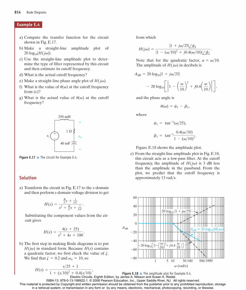
b) Make a straight-line amplitude plot of.

c) Use the straight-line amplitude plot to deter-mine the type of filter represented by this circuitand then estimate its cutoff frequency.

d) What is the actual cutoff frequency?

e) Make a straight-line phase angle plot of .

f) What is the value of at the cutoff frequencyfrom (c)?

g) What is the actual value of at the cutofffrequency?

u(v)

u(v)

H( jv)

20 log10|H( jv)|

from which

Note that for the quadratic factor,The amplitude of in decibels is

and the phase angle is

where

Figure E.18 shows the amplitude plot.

c) From the straight-line amplitude plot in Fig. E.18,this circuit acts as a low-pass filter. At the cutofffrequency, the amplitude of is 3 dB lessthan the amplitude in the passband. From theplot, we predict that the cutoff frequency isapproximately .13 rad>s

H( jv)

b1 = tan-10.4(v>10)

1 - (v>10)2 .

c1 = tan-1(v>25),

u(v) = c1 - b1,

- 20 log10B 2 1 - a v10b2

+ j0.4a v10b 2 R ,

AdB = 20 log10|1 + jv>25|

H( jv)u = v>10.

H(jv) =

|1 + jv>25|lc1

|1 - (v>10)2+ j0.4(v>10)|lb1

.

20 log10 �1 � jv/25�

�80

�60

�40

�20

0

20

40

60

AdB

1 10 100 100050050v (rad/s)

5

AdB � 20 log10�H( j�)�

�20 log10 �1� � j0.4 � 10v

10v2

Figure E.18 � The amplitude plot for Example E.4.

Solution

a) Transform the circuit in Fig. E.17 to the s-domainand then perform s-domain voltage division to get

Substituting the component values from the cir-cuit gives

b) The first step in making Bode diagrams is to putin standard form. Because contains

a quadratic factor, we first check the value of .We find that and , so

H(s) =

s>25 + 1

1 + (s>10)2+ 0.4(s>10)

,

vn = 10z = 0.2z

H(s)H(jv)

H(s) =

4(s + 25)

s2+ 4s + 100

.

H(s) =

RLs +

1LC

s2+

RLs +

1LC

.

89251_23_AppE 4/4/07 1:13 PM Page 814



E.8 Phase Angle Plots 815

d) To solve for the actual cutoff frequency, replace swith in , compute the expression for

, set ,and solve for . First,

Then,

Solving for gives us

e) Figure E.19 shows the phase angle plot. Notethat the straight-line segment of between1.0 and does not have the same slope asthe segment between 2.5 and .

f) From the phase angle plot in Fig. E.19, we esti-mate the phase angle at the cutoff frequency of

to be .

g) We can compute the exact phase angle at thecutoff frequency by substituting into thetransfer function :

H( j16) =

4( j16 + 25)

( j16)2+ 4( j16) + 100

.

H(s)s = j16

-65 �16 rad>s

100 rad>s2.5 rad>s u(v)

vc = 16 rad>s.

vc

|H( jvc)| =

2(4vc)2

+ 1002

2(100 - vc2)2

+ (4vc)2

=

112

.

H( jv) =

4( jv) + 100

( jv)2+ 4( jv) + 100

.

vc

Hmax = 1>12|H( jvc)| = (1>12 )|H( jv)|H(s)jv

Computing the phase angle, we see

Note the large error in the predicted angle. Ingeneral, straight-line phase angle plots do notgive satisfactory results in the frequency bandwhere the phase angle is changing. The straight-line phase angle plot is useful only in predictingthe general behavior of the phase angle, not inestimating actual phase angle values at particu-lar frequencies.

u(vc) = u( j16) = -125.0 � .

c1(v)

u (v)

�b1(v)

�180�

�135�

�90�

�45�

0�

45�

90�

135�

1 10 100 100050050v (rad/s)

u (v)

5

Figure E.19 � The phase angle plot for Example E.4.

89251_23_AppE 4/4/07 1:13 PM Page 815



89251_23_AppE 4/4/07 1:13 PM Page 816



Documents

89251 23 AppE 4/4/07 1:11 PM Page 799 Appendix Bode Diagrams