Embed Size (px)
Citation preview
8th lecture:Climate models
(Structure of climate models, components, climate scenarios: from past to the future)
Climate II (Winter 2020/2021)
Gerrit Lohmann, Martin Werner
Tuesday, 10:00-11:45(sometimes shorter, but with some exercises)
https://paleodyn.uni-bremen.de/study/climate2020_21.html
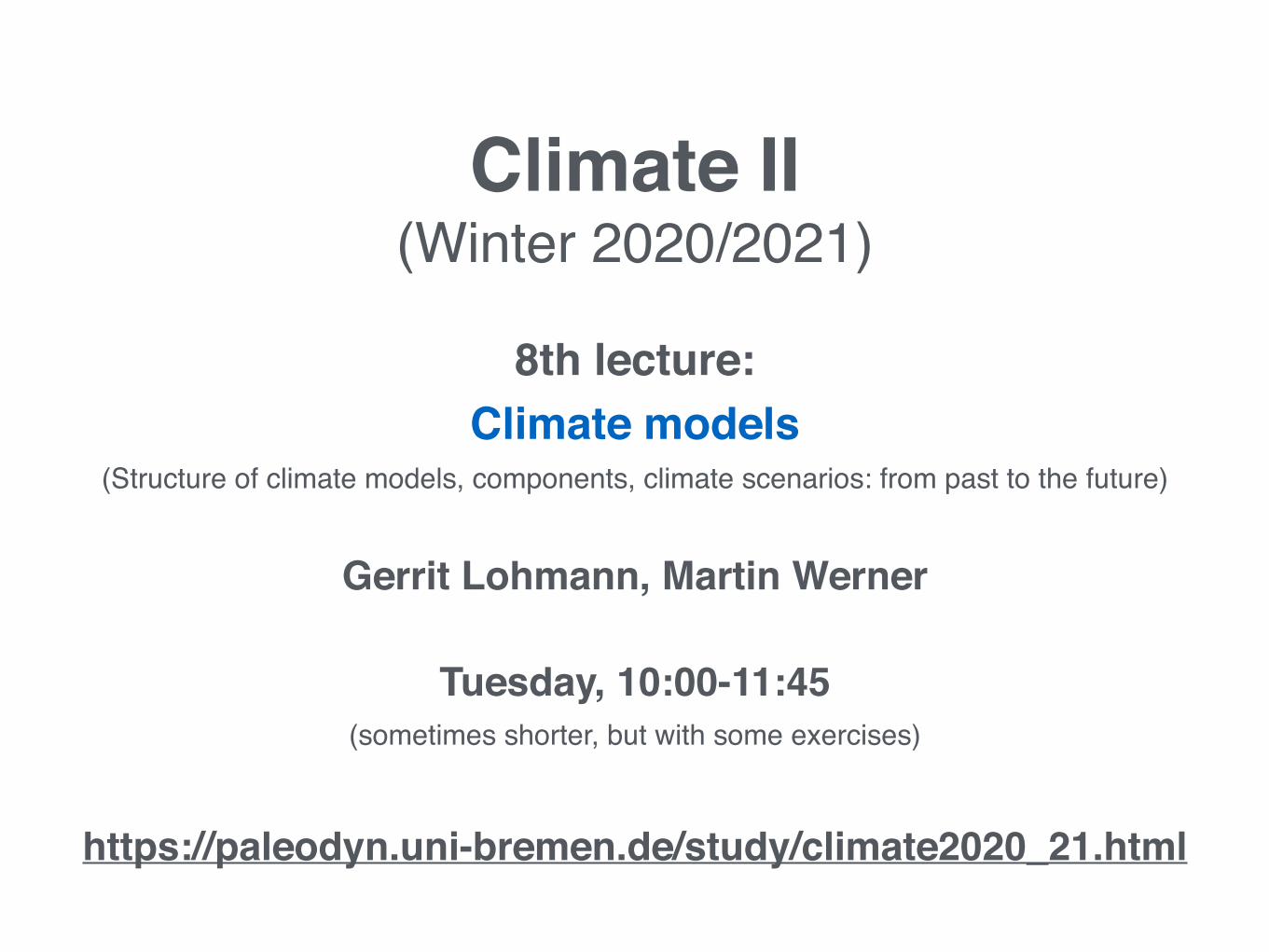
Dust in the climate systemRepetition
RepetitionDust depositions on glacial-interglacial time scalesLETTERS
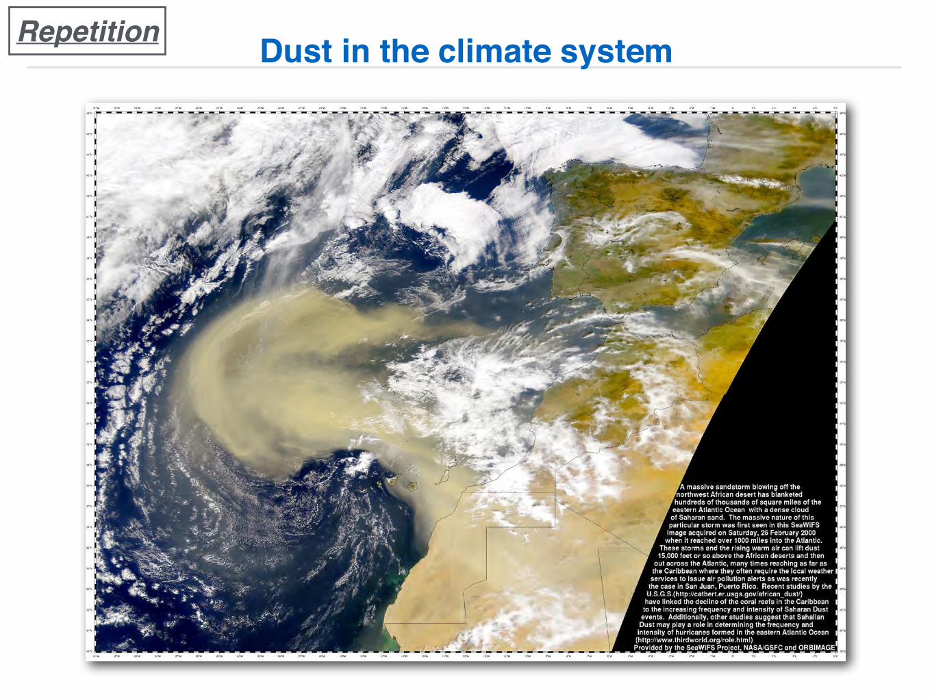
Dust2climate couplings over the past 800,000 yearsfrom the EPICA Dome C ice coreF. Lambert1,2, B. Delmonte3, J. R. Petit4, M. Bigler1,5, P. R. Kaufmann1,2, M. A. Hutterli6, T. F. Stocker1,2, U. Ruth7,J. P. Steffensen5 & V. Maggi3
Dust can affect the radiative balance of the atmosphere by absorb-ing or reflecting incoming solar radiation1; it can also be a sourceof micronutrients, such as iron, to the ocean2. It has been sug-gested that production, transport and deposition of dust is influ-enced by climatic changes on glacial2interglacial timescales3–6.Here we present a high-resolution record of aeolian dust fromthe EPICA Dome C ice core in East Antarctica, which providesan undisturbed climate sequence over the past eight climaticcycles7,8. We find that there is a significant correlation betweendust flux and temperature records during glacial periods that isabsent during interglacial periods. Our data suggest that dust fluxis increasingly correlated with Antarctic temperature as the cli-mate becomes colder. We interpret this as progressive coupling ofthe climates of Antarctic and lower latitudes. Limited changes inglacial2interglacial atmospheric transport time4,9,10 suggest thatthe sources and lifetime of dust are the main factors controllingthe high glacial dust input. We propose that the observed 25-foldincrease in glacial dust flux over all eight glacial periods can beattributed to a strengthening of South American dust sources,together with a longer lifetime for atmospheric dust particles inthe upper troposphere resulting from a reduced hydrological cycleduring the ice ages.
The EPICA (European Project for Ice Coring in Antarctica) icecore drilled at Dome C (hereafter EDC) in East Antarctica (75u 069 S;123u 219 E) covers the past 800,000 yr (Fig. 1a). The dust flux recordof Vostok (Fig. 1b) is thus extended over four additional cycles(Fig. 1c). The glacial–interglacial climate changes are well reflectedin the sequence of high and low dust concentrations with typicalvalues from 800 to 15 mg kg21 and a ratio of 50 to 1 over most ofthe past eight climate cycles. The concentration of insoluble dust insnow depends on a number of factors such as the primary supply ofsmall mineral particles from the continents, which is related to cli-mate and environmental conditions in the source region11, the snowaccumulation rate, the long-range transport, and the cleansing of theatmosphere associated with the hydrological cycle. The strontiumand neodymium isotopic signature of dust12 revealed that southernSouth America was the dominant dust source for East Antarcticaduring glacial times13, although contributions from other sourcesare possible during interglacials14. Because of the low accumulationrate at Dome C (,3 cm yr21 water equivalent), dry deposition isdominant and the atmospheric dust load is best represented by thedust flux15. The total dust flux and the magnitude of the glacial–interglacial changes are remarkably uniform within the EastAntarctic Plateau, as shown by the similarity between the EDC andthe Vostok records (Fig. 1b, despite some chronological differences
and a 10-times finer resolution at EDC) over the past four climaticcycles and also depicted by the Dome Fuji dust record16 (not shown).
At EDC, interglacials display dust fluxes similar to that of theHolocene (,400 mg m22 yr21). However, some differences can beseen in the record before and after the Mid-Brunhes Event (MBE,,430 kyr BP) which is considered a transition in the climatic record7,8
from cooler (for example Marine Isotopic Stages, MIS 13, 15, 17) towarmer (for example MIS 11, 9 and 5.5) interglacials. Before the MBEthere were fewer occurrences of low concentrations, and warmperiods represent ,12% of the time, compared with ,30% afterthe MBE. All eight glacial periods appear similar in magnitude andshow an average increase in dust flux by a factor of about 25, withglacial maxima displaying fluxes of at least 12 mg m22 yr21. Theweakest glacial stages in the EDC ice core are MIS 14 and 16. ForMIS 14 this is consistent with the findings from terrestrial and marinerecords6,17,18. In contrast, MIS 16 in those records is the strongestglacial in the Late Quaternary period.
The extension of the EDC dust record to 800 kyr BP confirms theincreased atmospheric dust load during cold periods of theQuaternary period with respect to warm stages. The first-ordersimilarity of EDC dust with the global ice-volume record (Fig. 1e,r2 5 0.6) confirms that major aeolian deflation in the SouthernHemisphere was linked to Pleistocene glaciations. Comparison withthe magnetic susceptibility record of loess/palaeosol sequences fromthe Chinese Loess Plateau (Fig. 1f) also provides evidence for broadsynchronicity of global changes in atmospheric dust load.
EDC dust has been measured using both a Coulter counter and alaser sensor (see Methods). Laser measurements are obtained athigher resolution along the core, but dust size is difficult to calibrate;therefore only the relative variation of the signal is used. Overall, theCoulter counter and laser (relative) size records (Fig. 1d) are in goodagreement. The slight discrepancies during MIS 5.5, 6 and 12 arepossibly related to the different sampling resolution, as size data fromthe laser and Coulter counter represent a continuous 1.1-m averageand discrete 7-cm subsamples every 0.5–6 m, respectively. From MIS14 (,2,900 m depth) and downwards in the ice core, the dust sizeprofile is not available because of the presence of particle aggregatesformed in the ice. This phenomenon, which needs further investiga-tion, has been observed in the EDC core only in very deep glacialsections, where ice thinning becomes very important and in situtemperature higher than 28 uC may allow partial melting aroundparticles. This problem was solved through sonication of the samples,which allowed us to obtain reliable concentration data (seeMethods). For the upper part of the record, larger (smaller) particlesare generally observed during warm (cold) periods, as reflected by the
1Climate and Environmental Physics, Physics Institute, University of Bern, Sidlerstrasse 5, 3012 Bern, Switzerland. 2Oeschger Centre for Climate Change Research, University of Bern,3012 Bern, Switzerland. 3Environmental Sciences Department, University of Milano Bicocca, Piazza della Scienza 1, 20126 Milano, Italy. 4Laboratoire de Glaciologie et Geophysique del’Environment (LGGE), CNRS-University J. Fourier, BP96 38402 Saint-Martin-d’Heres cedex, France. 5Centre for Ice and Climate, Niels Bohr Institute, University of Copenhagen,Juliane Maries Vej 30, 2100 Copenhagen OE, Denmark. 6British Antarctic Survey, High Cross, Madingley Road, Cambridge CB3 0ET, UK. 7Alfred Wegener Institute for Polar andMarine Research, Columbusstrasse, 27568 Bremerhaven, Germany.
Vol 452 | 3 April 2008 | doi:10.1038/nature06763
616Nature Publishing Group©2008
LETTERS
Dust2climate couplings over the past 800,000 yearsfrom the EPICA Dome C ice coreF. Lambert1,2, B. Delmonte3, J. R. Petit4, M. Bigler1,5, P. R. Kaufmann1,2, M. A. Hutterli6, T. F. Stocker1,2, U. Ruth7,J. P. Steffensen5 & V. Maggi3
Dust can affect the radiative balance of the atmosphere by absorb-ing or reflecting incoming solar radiation1; it can also be a sourceof micronutrients, such as iron, to the ocean2. It has been sug-gested that production, transport and deposition of dust is influ-enced by climatic changes on glacial2interglacial timescales3–6.Here we present a high-resolution record of aeolian dust fromthe EPICA Dome C ice core in East Antarctica, which providesan undisturbed climate sequence over the past eight climaticcycles7,8. We find that there is a significant correlation betweendust flux and temperature records during glacial periods that isabsent during interglacial periods. Our data suggest that dust fluxis increasingly correlated with Antarctic temperature as the cli-mate becomes colder. We interpret this as progressive coupling ofthe climates of Antarctic and lower latitudes. Limited changes inglacial2interglacial atmospheric transport time4,9,10 suggest thatthe sources and lifetime of dust are the main factors controllingthe high glacial dust input. We propose that the observed 25-foldincrease in glacial dust flux over all eight glacial periods can beattributed to a strengthening of South American dust sources,together with a longer lifetime for atmospheric dust particles inthe upper troposphere resulting from a reduced hydrological cycleduring the ice ages.
The EPICA (European Project for Ice Coring in Antarctica) icecore drilled at Dome C (hereafter EDC) in East Antarctica (75u 069 S;123u 219 E) covers the past 800,000 yr (Fig. 1a). The dust flux recordof Vostok (Fig. 1b) is thus extended over four additional cycles(Fig. 1c). The glacial–interglacial climate changes are well reflectedin the sequence of high and low dust concentrations with typicalvalues from 800 to 15 mg kg21 and a ratio of 50 to 1 over most ofthe past eight climate cycles. The concentration of insoluble dust insnow depends on a number of factors such as the primary supply ofsmall mineral particles from the continents, which is related to cli-mate and environmental conditions in the source region11, the snowaccumulation rate, the long-range transport, and the cleansing of theatmosphere associated with the hydrological cycle. The strontiumand neodymium isotopic signature of dust12 revealed that southernSouth America was the dominant dust source for East Antarcticaduring glacial times13, although contributions from other sourcesare possible during interglacials14. Because of the low accumulationrate at Dome C (,3 cm yr21 water equivalent), dry deposition isdominant and the atmospheric dust load is best represented by thedust flux15. The total dust flux and the magnitude of the glacial–interglacial changes are remarkably uniform within the EastAntarctic Plateau, as shown by the similarity between the EDC andthe Vostok records (Fig. 1b, despite some chronological differences
and a 10-times finer resolution at EDC) over the past four climaticcycles and also depicted by the Dome Fuji dust record16 (not shown).
At EDC, interglacials display dust fluxes similar to that of theHolocene (,400 mg m22 yr21). However, some differences can beseen in the record before and after the Mid-Brunhes Event (MBE,,430 kyr BP) which is considered a transition in the climatic record7,8
from cooler (for example Marine Isotopic Stages, MIS 13, 15, 17) towarmer (for example MIS 11, 9 and 5.5) interglacials. Before the MBEthere were fewer occurrences of low concentrations, and warmperiods represent ,12% of the time, compared with ,30% afterthe MBE. All eight glacial periods appear similar in magnitude andshow an average increase in dust flux by a factor of about 25, withglacial maxima displaying fluxes of at least 12 mg m22 yr21. Theweakest glacial stages in the EDC ice core are MIS 14 and 16. ForMIS 14 this is consistent with the findings from terrestrial and marinerecords6,17,18. In contrast, MIS 16 in those records is the strongestglacial in the Late Quaternary period.
The extension of the EDC dust record to 800 kyr BP confirms theincreased atmospheric dust load during cold periods of theQuaternary period with respect to warm stages. The first-ordersimilarity of EDC dust with the global ice-volume record (Fig. 1e,r2 5 0.6) confirms that major aeolian deflation in the SouthernHemisphere was linked to Pleistocene glaciations. Comparison withthe magnetic susceptibility record of loess/palaeosol sequences fromthe Chinese Loess Plateau (Fig. 1f) also provides evidence for broadsynchronicity of global changes in atmospheric dust load.
EDC dust has been measured using both a Coulter counter and alaser sensor (see Methods). Laser measurements are obtained athigher resolution along the core, but dust size is difficult to calibrate;therefore only the relative variation of the signal is used. Overall, theCoulter counter and laser (relative) size records (Fig. 1d) are in goodagreement. The slight discrepancies during MIS 5.5, 6 and 12 arepossibly related to the different sampling resolution, as size data fromthe laser and Coulter counter represent a continuous 1.1-m averageand discrete 7-cm subsamples every 0.5–6 m, respectively. From MIS14 (,2,900 m depth) and downwards in the ice core, the dust sizeprofile is not available because of the presence of particle aggregatesformed in the ice. This phenomenon, which needs further investiga-tion, has been observed in the EDC core only in very deep glacialsections, where ice thinning becomes very important and in situtemperature higher than 28 uC may allow partial melting aroundparticles. This problem was solved through sonication of the samples,which allowed us to obtain reliable concentration data (seeMethods). For the upper part of the record, larger (smaller) particlesare generally observed during warm (cold) periods, as reflected by the
1Climate and Environmental Physics, Physics Institute, University of Bern, Sidlerstrasse 5, 3012 Bern, Switzerland. 2Oeschger Centre for Climate Change Research, University of Bern,3012 Bern, Switzerland. 3Environmental Sciences Department, University of Milano Bicocca, Piazza della Scienza 1, 20126 Milano, Italy. 4Laboratoire de Glaciologie et Geophysique del’Environment (LGGE), CNRS-University J. Fourier, BP96 38402 Saint-Martin-d’Heres cedex, France. 5Centre for Ice and Climate, Niels Bohr Institute, University of Copenhagen,Juliane Maries Vej 30, 2100 Copenhagen OE, Denmark. 6British Antarctic Survey, High Cross, Madingley Road, Cambridge CB3 0ET, UK. 7Alfred Wegener Institute for Polar andMarine Research, Columbusstrasse, 27568 Bremerhaven, Germany.
Vol 452 | 3 April 2008 | doi:10.1038/nature06763
616Nature Publishing Group©2008
variability in the fine particle percentage (FPP)12, which is highestduring the two last glacial periods. The advection of dust to centralAntarctica involves the high levels of the troposphere and the smallchanges in dust size may reflect changes in the altitude of transportand thus transport time12. Higher FPP values in glacial times havebeen ultimately attributed to increased isolation of Dome C duringglacials, in terms of reduced dust transport associated with greatersubsidence12 or possibly through baroclinic eddies.
Comparing dust and stable isotope (dD) profiles, there is a signifi-cant correlation during glacial periods (Fig. 2), and up to 90% of thedust variability can be explained by the temperature variations. Inglacial periods, most of the dD events (for example, AntarcticIsotopic Maxima) have their counterparts in the dust data shownby a reduction of dust concentrations. In contrast, dust and temper-ature records are not correlated during interglacial periods (Fig. 2).Indeed, the (logarithmic) relationship between dust flux and dD can
8006004002000
4.8
4
3.2
Mar
ine
δ18 O
(%0)
–2
0
2
Chi
nese
loes
sm
agn.
sus
c.(n
orm
.)
2
1
0
–1
–2
–3
EDC
dus
tFP
P (n
orm
.)
10
1
0.1
EDC
dus
tflu
x (m
g m
–2 y
r–1 )
10
1
0.1
Vost
ok d
ust
flux
(mg
m–2
yr–
1 ) –440
–400
–360
EDC
δD
(%0)
a
b
c
d
e
f
191715.1131197.55.5
Coarse
Fine
1614
Age (kyr)
Figure 1 | EDC dust data in comparison with other climatic indicators.a, Stable isotope (dD) record from the EPICA Dome C (EDC) ice core8 backto Marine Isotopic Stage 20 (EDC3 timescale) showing Quaternarytemperature variations in Antarctica. b, Vostok dust flux record (Coultercounter) plotted on its original timescale11. c, EDC dust flux records. Redand grey lines represent, respectively, Coulter counter (55-cm to 6-mresolution) and laser-scattering data (55-cm mean). Numbers indicate
Marine Isotopic Stages. Note that the vertical extent of the scales of b and c islarger than for the other records. d, EDC dust size data expressed as FPP (seeMethods). The orange and grey curves represent measurements by Coultercounter (2-kyr mean) and laser (1-kyr mean), respectively. e, Marinesediment d18O stack18, giving the pattern of global ice volume. f, Magneticsusceptibility stack record for Chinese loess17 (normalized).
8006004002000
Age (kyr)
0
0.2
0.4
0.6
0.8
1.0
r2
0
5
10
15
20
25
EDC
dus
t flu
x (m
g m
–2 y
r–1 )
146LGM 181612108
Figure 2 | EDC correlation between dust and temperature. Linear plot ofdust flux (black) and the coefficient of determination r2 (blue) between thehigh-pass filtered values (18-kyr cut-off) of both the dD and the logarithmicvalues of dust flux. The correlation was determined using 2-kyr mean values
in both records and a gliding 22-kyr window. Correlations above r2 5 0.27(dashed line) are significant at a 95% confidence level. Numbers indicate themarine isotopic glacial stages.
NATURE | Vol 452 | 3 April 2008 LETTERS
617Nature Publishing Group©2008
be well fitted by a cubic polynomial (Fig. 3). Over the record, thegeometric standard deviation from the polynomial fit represents afactor of ,2 in concentrations independent of the climatic period.Similarly, this relationship does not change before and after the MBE.The crescent shape of the dust–dD relationship suggests that the dustfluxes have a higher temperature sensitivity as the climate becomescolder. For dD values above about –405%, Antarctic temperatureand dust flux are not correlated, whereas there is a clear correlationfor dD values below about –425%. This behaviour may represent theexpression of a progressive coupling between high- and low-latitudeclimate as temperatures become colder. During extreme glacial con-ditions the coupling appears as a direct influence of the Antarctic onthe climate of southern South America19,20. The coupling of Antarcticand lower-latitude climate is probably coincident with the signifi-cantly extended sea ice over the Southern Atlantic and the SouthernOcean during glacials21 and the consequent meridional (northward)shift of the atmospheric circulation (that is, the westerlies)19–22.
Questions remain about the main factors influencing the high dustinput into polar areas during glacial periods. So far, general circula-tion models4,10 have reproduced a glacial dust transport and flux overtropical and mid-latitude regions which is in good agreement withglobal reconstructions3, but they have failed to simulate the 25-foldincrease observed in glacial dust input over Antarctica. This short-coming is currently attributed to an incomplete representation of thesource strength23. In addition, most of the models suggest modestchanges in atmospheric transport4,9,10, which seems supported by therelatively small changes in dust size in the EDC ice core, and by thecomparison of the two EPICA ice cores24. Moreover, the suggestionthat the 25-fold dust influx increase is mainly due to changes insource strength is challenged by evidence from South Atlantic marinerecords suggesting a 5- to 10-fold increase in the South Americansource strength25,26 during the last glacial period.
On the basis of the new EDC data set, we suggest a new hypothesisfor the glacial–interglacial changes in transport of dust. The indica-tion (Fig. 3) that Antarctica and the southern low latitudes experi-enced a different coupling during the past 800 kyr is closely linkedwith the dust pathway within the high troposphere and the likely
extended lifetime. With respect to the dust emitted from continents,the dust arriving in Antarctica, with a mode around 2 mm diameter27,represents the endmember of the distribution. The small size of dustparticles makes en route gravitational settling inefficient (very longdry deposition lifetime), allowing mixing and spreading at high alti-tude within the troposphere. The lifetime of the particles is primarilyconstrained by wet deposition23,28 and therefore by water content andtemperature. As an example, along a pathway 4–6 km high and with amean temperature of about –40 uC (conditions similar to thoseobserved over Antarctica), a temperature reduction by 5 uC, assoc-iated with a similar change of sea surface temperature over theSouthern Ocean29, reduces the saturation water vapour pressure toabout half. Under such premises, a two-dimensional model28
obtained an increase in dust flux to Antarctica of up to a factor of5. Thus the roughly 25-fold increase in dust flux over the Antarcticplateau during glacials could be explained by a progressive couplingof the climate of Antarctic and lower latitudes with colder tempera-tures, one influencing the other, and leading to the stronger aeoliandeflation of southern South America and to a significantly increaseddust particle lifetime along their pathway in the high-altitude tro-posphere over the Southern Ocean. The new EDC data set thusprovides important constraints for models of the dust cycle duringglacial–interglacial cycles.
METHODS SUMMARYApparatus. Samples for Coulter Counter Multisizer IIe measurements wereobtained from discrete samples (7 cm long), decontaminated at LGGE throughwashing in ultrapure water. We adopted the analytical procedure described inref. 12 (and references therein). A total of about 1,100 values have been obtained.
We obtained laser scattering data from the University of Copenhagen devicefor the section between 0 and 770 m. The University of Bern device was usedbetween 770 and 3,200 m. Data from both devices were calibrated by Coultercounter. Sampling resolution is about 1 cm.Particle size distribution. Dust size is expressed as FPP. We define FPP accord-ing to ref. 12 as the proportion of the mass of particles having diameter between 1and 2mm with respect to the total mass of the sample, which typically includesparticles in the size range 1 to 5mm. This parameter is inversely correlated withthe modal value of the log-normal dust mass (volume) size distribution.
From a depth of 2,900 m and below, some glacial samples show distributionswith an anomalously large mode. This has been attributed to particle aggregateformation in ice (Supplementary Fig. 1) and prompted us to discard all sizedistribution data below that point until this phenomenon is better understood.To obtain reliable dust mass, samples were submitted to ultrasonic treatment tobreak the aggregates apart. Between 3,139-m and 3,190-m depth, 42 sampleswith anomalous size distribution were submitted to ultrasonic treatment. For 39of these we accepted the new dust mass measurement, with 11 samples showing asignificantly different mass value (Supplementary Table 1). Measurement on afew chosen samples above 3,139-m depth showed normal size distribution andconcentration values. However, additional measurements are scheduled for in-depth analysis of the aggregate problem.
Received 14 May 2007; accepted 21 January 2008.
1. Tegen, I. Modeling the mineral dust aerosol cycle in the climate system. Quat. Sci.Rev. 22, 1821–1834 (2003).
2. Fung, I. et al. Iron supply and demand in the upper ocean. Glob. Biogeochem. Cycles14, 281–296 (2000).
3. Kohfeld, K. E. & Harrison, S. P. DIRTMAP: the geological record of dust. Earth Sci.Rev. 54, 81–114 (2001).
4. Mahowald, N. et al. Dust sources and deposition during the last glacial maximumand current climate: A comparison of model results with paleodata from ice coresand marine sediments. J. Geophys. Res. 104, 15895–15916 (1999).
5. Steffensen, J. P. The size distribution of microparticles from selected segments ofthe Greenland Ice Core Project ice core representing different climatic periods.J. Geophys. Res. 102, 26755–26763 (1997).
6. Sun, Y. B., Clemens, S. C., An, Z. S. & Yu, Z. W. Astronomical timescale andpalaeoclimatic implication of stacked 3.6-Myr monsoon records from theChinese Loess Plateau. Quat. Sci. Rev. 25, 33–48 (2006).
7. EPICA community members. Eight glacial cycles from an Antarctic ice core.Nature 429, 623–628 (2004).
8. Jouzel, J. et al. Orbital and millennial Antarctic variability over the last 800 000years. Science 317, doi:10.1126/science.1141038 (2007).
9. Krinner, G. & Genthon, C. Tropospheric transport of continental tracers towardsAntarctica under varying climatic conditions. Tellus 55B, 54–70 (2003).
–360–380–400–420–440–460δD (%0)
0.1
1
10
EDC
dus
t flu
x (m
g m
–2 y
r–1 )
EDC dust flux 0–430 kyr BP
EDC dust flux 430–800 kyr BP
InterglacialGlacial
Figure 3 | EDC dust–temperature relationship. Values of dD (ref. 8) areplotted against dust flux (both at 55-cm resolution). Green and blue dotsrepresent data from 0–430 kyr BP and 430–800 kyr BP, respectively.Superposed is a cubic polynomial fit,log10(f) 5 23.737 3 1026(dD)3 2 4.239 3 1023(dD)2 2 1.607(dD) 2 204,where f is the dust flux (mg m22 yr21), and dD is in% (r2 5 0.73, N 5 5,164).
LETTERS NATURE | Vol 452 | 3 April 2008
618Nature Publishing Group©2008
• strong correlation between dust and temperature changes
RepetitionDust depositions on glacial-interglacial time scales
correlates with the deepest part of the sedimen-tary basin.
The predicted ground motion is qualitativelysimilar for the VEA and CyberShake simulations(figs. S4 and S5); however, there are substantialquantitative differences in the level and distribu-tion of the shaking (Fig. 4). SAVELA resultsshow stronger shaking than CyberShake at mostsites. This is especially true for receivers in thebasin. We note that both methods are subject tosubstantial uncertainties. The accuracy of theCyberShake simulations depends strongly on theaccuracy of the assumed crustal velocity modeland its derived Green’s functions. The accuracyof the virtual earthquake results depends stronglyboth on the accuracy of the ambient-field Green’sfunctions and on the accuracy of the amplitudecalibration. The Green’s functions we used forthis study (fig. S1) would be more accurate if wehad data from a longer deployment. To estimatethe variability in PGV due to the amplitude cal-ibration described above, we measure the max-imum difference in predicted PGV when usingthe calibration from either the Hector Road orChino Hills earthquake to the mean of the cali-bration used in this study. The variability that re-sults is bounded at 10 cm/s for our simulations.For both the virtual earthquake and CyberShakesimulations, the variation of the PGV is narrowfor stations with low PGV values (bedrock sites)and wide for stations with high PGV values (basinsites). The coefficient of variation is approximate-ly constant for SAVELA (fig. S7), which indicatesthat variability increases proportionallywith groundmotion amplitude.
Nonlinear effects in shallow materials are im-portant in strong ground motion. Ground motionsimulations that have incorporated nonlinear soileffects (29) have found a large decrease in thepredicted strong groundmotion. This could be animportant effect for the scenarios we considerbecause unconsolidated sediments are likely to befound in sedimentary basins and would be ex-pected to behave nonlinearly during strong shaking.We calibrated the amplitudes of the Green’s func-tions, such that the peak amplitudes predictedby our approach matched those of moderate-sized earthquakes. Our approach, as well as theCyberShake simulations, is based on an assump-tion of linearity. To the extent that nonlinear ef-fects are important, our predicted ground motionamplitudes are likely to overestimate true ampli-tudes in future large earthquakes.
We confirm the presence and the influence ofa waveguide to the west of San Gorgonio Passthat funnels seismic waves from San Andreasfault events into the Los Angeles Basin. Thisamplification is present for all tested scenarios.We also confirm that directivity couples withshallow crustal structure to increase basin am-plification (6). We find a constant coefficient ofvariation, which means that shaking variabilityis proportional to shaking intensity. We also finda wider range of predicted peak amplitudes thanis found in simulations, which would increase
uncertainty in ground motion predictions andthereby impact seismic hazard assessments. Wenote, however, that there are substantial uncer-tainties in our estimated Green’s functions andtheir amplitude calibration. Moreover, station cov-erage in the basin is sparse, and we have onlysampled a small portion of the variability expectedfor a complex wavefield in the basin. Our resultssupport more ambitious, targeted experimentsto improve the accuracy of long-period strongground motion prediction for future earthquakesin regions subject to high seismic risk.
References and Notes1. P.-Y. Bard, M. Campillo, F. J. Chávez-Garcia,
F. J. Sánchez-Sesma, Earthq. Spectra 4, 609–633(1988).
2. K. B. Olsen, R. J. Archuleta, J. R. Matarese, Science 270,1628–1632 (1995).
3. K. Olsen et al., Geophys. Res. Lett. 33, L07305(2006).
4. K. B. Olsen et al., Geophys. Res. Lett. 36, L04303(2009).
5. K. B. Olsen, Bull. Seismol. Soc. Am. 90 (6B), S77–S94(2000).
6. R. Graves et al., Pure Appl. Geophys. 168, 367–381(2011).
7. S. M. Day, D. Roten, K. B. Olsen, Geophys. J. Int. 189,1103–1124 (2012).
8. K. Aki, Bull. Earthq. Res. I. Tokyo 35, 415 (1957).9. J. Claerbout, Geophysics 33, 264–269 (1968).10. O. I. Lobkis, R. L. Weaver, J. Acoust. Soc. Am. 110, 3011
(2001).11. R. L. Weaver, O. I. Lobkis, Geophysics 71, S15
(2006).12. F. J. Sánchez-Sesma, M. Campillo, Bull. Seismol. Soc. Am.
96, 1182–1191 (2006).13. M. Campillo, A. Paul, Science 299, 547–549 (2003).14. N. M. Shapiro, M. Campillo, Geophys. Res. Lett. 31,
L07614 (2004).15. K. G. Sabra, P. Gerstoft, P. Roux, W. A. Kuperman,
M. C. Fehler, Geophys. Res. Lett. 32, L03310(2005).
16. N. M. Shapiro, M. Campillo, L. Stehly, M. H. Ritzwoller,Science 307, 1615–1618 (2005).
17. K. Nishida, H. Kawakatsu, K. Obara, J. Geophys. Res. 113(B10), B10302 (2008).
18. G. A. Prieto, J. F. Lawrence, G. C. Beroza, J. Geophys. Res.114 (B7), B07303 (2009).
19. G. A. Prieto, M. Denolle, J. F. Lawrence, G. C. Beroza,C. R. Geosci. 343, 600–614 (2011).
20. G. A. Prieto, G. C. Beroza, Geophys. Res. Lett. 35, L14304(2008).
21. M. A. Denolle, E. M. Dunham, G. A. Prieto, G. C. Beroza,J. Geophys. Res. 118, 2102 (2013).
22. R. Burridge, L. Knopoff, Bull. Seismol. Soc. Am. 54,1875–1888 (1964).
23. H. Magistrale, S. Day, R. W. Clayton, R. Graves,Bull. Seismol. Soc. Am. 90 (6B), S65–S76 (2000).
24. M. D. Kohler, H. Magistrale, R. W. Clayton, Bull. Seismol.Soc. Am. 93, 757–774 (2003).
25. M. A. Denolle, E. M. Dunham, G. C. Beroza, Bull. Seismol.Soc. Am. 102, 1214–1223 (2012).
26. L. Stehly, M. Campillo, N. Shapiro, J. Geophys. Res. 111(B10), B10306 (2006).
27. M. Guatteri, P. M. Mai, G. C. Beroza, Bull. Seismol.Soc. Am. 94, 2051–2063 (2004).
28. K. W. Campbell, Y. Bozorgnia, Bull. Seismol. Soc. Am. 93,314–331 (2003).
29. D. Roten, K. B. Olsen, J. C. Pechmann, Bull. Seismol.Soc. Am. 102, 2008–2030 (2012).
Acknowledgments: We thank K. Olsen and anonymousreviewers for their comments and contributions to improvethe manuscript. This work was supported by NSF grantEAR-0943885 and by the Southern California EarthquakeCenter (SCEC). SCEC is funded by NSF cooperative agreementEAR-0529922 and U.S. Geological Survey cooperativeagreement 07HQAG0008. The SCEC contribution numberfor this paper is 1812. Data are available in the supplementarymaterials.
Supplementary Materialswww.sciencemag.org/content/343/6169/399/suppl/DC1Materials and MethodsFigs. S1 to S7References (30–33)
9 September 2013; accepted 19 December 201310.1126/science.1245678
Increased Dust Deposition in thePacific Southern Ocean DuringGlacial PeriodsF. Lamy,1,2* R. Gersonde,1,2 G. Winckler,3,4 O. Esper,1 A. Jaeschke,1,2 G. Kuhn,1 J. Ullermann,1
A. Martinez-Garcia,5 F. Lambert,6 R. Kilian7
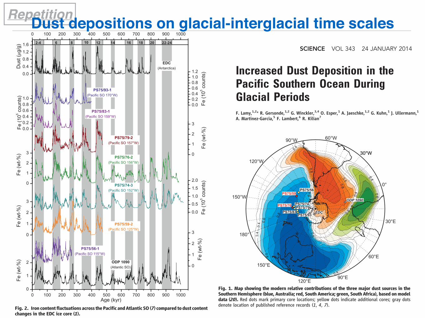
Dust deposition in the Southern Ocean constitutes a critical modulator of past global climatevariability, but how it has varied temporally and geographically is underdetermined. Here, wepresent data sets of glacial-interglacial dust-supply cycles from the largest Southern Ocean sector,the polar South Pacific, indicating three times higher dust deposition during glacial periodsthan during interglacials for the past million years. Although the most likely dust source for theSouth Pacific is Australia and New Zealand, the glacial-interglacial pattern and timing of lithogenicsediment deposition is similar to dust records from Antarctica and the South Atlantic dominatedby Patagonian sources. These similarities imply large-scale common climate forcings, such aslatitudinal shifts of the southern westerlies and regionally enhanced glaciogenic dust mobilizationin New Zealand and Patagonia.
Mineral aerosols (dust) play a crucial rolein determining the pattern and mag-nitude of climate variability. Dust im-
purities trapped in Antarctic ice point to ~25 timeshigher glacial dust fluxes compared with inter-glacials (1). It has been suggested that an increase
www.sciencemag.org SCIENCE VOL 343 24 JANUARY 2014 403
REPORTS
correlates with the deepest part of the sedimen-tary basin.
The predicted ground motion is qualitativelysimilar for the VEA and CyberShake simulations(figs. S4 and S5); however, there are substantialquantitative differences in the level and distribu-tion of the shaking (Fig. 4). SAVELA resultsshow stronger shaking than CyberShake at mostsites. This is especially true for receivers in thebasin. We note that both methods are subject tosubstantial uncertainties. The accuracy of theCyberShake simulations depends strongly on theaccuracy of the assumed crustal velocity modeland its derived Green’s functions. The accuracyof the virtual earthquake results depends stronglyboth on the accuracy of the ambient-field Green’sfunctions and on the accuracy of the amplitudecalibration. The Green’s functions we used forthis study (fig. S1) would be more accurate if wehad data from a longer deployment. To estimatethe variability in PGV due to the amplitude cal-ibration described above, we measure the max-imum difference in predicted PGV when usingthe calibration from either the Hector Road orChino Hills earthquake to the mean of the cali-bration used in this study. The variability that re-sults is bounded at 10 cm/s for our simulations.For both the virtual earthquake and CyberShakesimulations, the variation of the PGV is narrowfor stations with low PGV values (bedrock sites)and wide for stations with high PGV values (basinsites). The coefficient of variation is approximate-ly constant for SAVELA (fig. S7), which indicatesthat variability increases proportionallywith groundmotion amplitude.
Nonlinear effects in shallow materials are im-portant in strong ground motion. Ground motionsimulations that have incorporated nonlinear soileffects (29) have found a large decrease in thepredicted strong groundmotion. This could be animportant effect for the scenarios we considerbecause unconsolidated sediments are likely to befound in sedimentary basins and would be ex-pected to behave nonlinearly during strong shaking.We calibrated the amplitudes of the Green’s func-tions, such that the peak amplitudes predictedby our approach matched those of moderate-sized earthquakes. Our approach, as well as theCyberShake simulations, is based on an assump-tion of linearity. To the extent that nonlinear ef-fects are important, our predicted ground motionamplitudes are likely to overestimate true ampli-tudes in future large earthquakes.
We confirm the presence and the influence ofa waveguide to the west of San Gorgonio Passthat funnels seismic waves from San Andreasfault events into the Los Angeles Basin. Thisamplification is present for all tested scenarios.We also confirm that directivity couples withshallow crustal structure to increase basin am-plification (6). We find a constant coefficient ofvariation, which means that shaking variabilityis proportional to shaking intensity. We also finda wider range of predicted peak amplitudes thanis found in simulations, which would increase
uncertainty in ground motion predictions andthereby impact seismic hazard assessments. Wenote, however, that there are substantial uncer-tainties in our estimated Green’s functions andtheir amplitude calibration. Moreover, station cov-erage in the basin is sparse, and we have onlysampled a small portion of the variability expectedfor a complex wavefield in the basin. Our resultssupport more ambitious, targeted experimentsto improve the accuracy of long-period strongground motion prediction for future earthquakesin regions subject to high seismic risk.
References and Notes1. P.-Y. Bard, M. Campillo, F. J. Chávez-Garcia,
F. J. Sánchez-Sesma, Earthq. Spectra 4, 609–633(1988).
2. K. B. Olsen, R. J. Archuleta, J. R. Matarese, Science 270,1628–1632 (1995).
3. K. Olsen et al., Geophys. Res. Lett. 33, L07305(2006).
4. K. B. Olsen et al., Geophys. Res. Lett. 36, L04303(2009).
5. K. B. Olsen, Bull. Seismol. Soc. Am. 90 (6B), S77–S94(2000).
6. R. Graves et al., Pure Appl. Geophys. 168, 367–381(2011).
7. S. M. Day, D. Roten, K. B. Olsen, Geophys. J. Int. 189,1103–1124 (2012).
8. K. Aki, Bull. Earthq. Res. I. Tokyo 35, 415 (1957).9. J. Claerbout, Geophysics 33, 264–269 (1968).10. O. I. Lobkis, R. L. Weaver, J. Acoust. Soc. Am. 110, 3011
(2001).11. R. L. Weaver, O. I. Lobkis, Geophysics 71, S15
(2006).12. F. J. Sánchez-Sesma, M. Campillo, Bull. Seismol. Soc. Am.
96, 1182–1191 (2006).13. M. Campillo, A. Paul, Science 299, 547–549 (2003).14. N. M. Shapiro, M. Campillo, Geophys. Res. Lett. 31,
L07614 (2004).15. K. G. Sabra, P. Gerstoft, P. Roux, W. A. Kuperman,
M. C. Fehler, Geophys. Res. Lett. 32, L03310(2005).
16. N. M. Shapiro, M. Campillo, L. Stehly, M. H. Ritzwoller,Science 307, 1615–1618 (2005).
17. K. Nishida, H. Kawakatsu, K. Obara, J. Geophys. Res. 113(B10), B10302 (2008).
18. G. A. Prieto, J. F. Lawrence, G. C. Beroza, J. Geophys. Res.114 (B7), B07303 (2009).
19. G. A. Prieto, M. Denolle, J. F. Lawrence, G. C. Beroza,C. R. Geosci. 343, 600–614 (2011).
20. G. A. Prieto, G. C. Beroza, Geophys. Res. Lett. 35, L14304(2008).
21. M. A. Denolle, E. M. Dunham, G. A. Prieto, G. C. Beroza,J. Geophys. Res. 118, 2102 (2013).
22. R. Burridge, L. Knopoff, Bull. Seismol. Soc. Am. 54,1875–1888 (1964).
23. H. Magistrale, S. Day, R. W. Clayton, R. Graves,Bull. Seismol. Soc. Am. 90 (6B), S65–S76 (2000).
24. M. D. Kohler, H. Magistrale, R. W. Clayton, Bull. Seismol.Soc. Am. 93, 757–774 (2003).
25. M. A. Denolle, E. M. Dunham, G. C. Beroza, Bull. Seismol.Soc. Am. 102, 1214–1223 (2012).
26. L. Stehly, M. Campillo, N. Shapiro, J. Geophys. Res. 111(B10), B10306 (2006).
27. M. Guatteri, P. M. Mai, G. C. Beroza, Bull. Seismol.Soc. Am. 94, 2051–2063 (2004).
28. K. W. Campbell, Y. Bozorgnia, Bull. Seismol. Soc. Am. 93,314–331 (2003).
29. D. Roten, K. B. Olsen, J. C. Pechmann, Bull. Seismol.Soc. Am. 102, 2008–2030 (2012).
Acknowledgments: We thank K. Olsen and anonymousreviewers for their comments and contributions to improvethe manuscript. This work was supported by NSF grantEAR-0943885 and by the Southern California EarthquakeCenter (SCEC). SCEC is funded by NSF cooperative agreementEAR-0529922 and U.S. Geological Survey cooperativeagreement 07HQAG0008. The SCEC contribution numberfor this paper is 1812. Data are available in the supplementarymaterials.
Supplementary Materialswww.sciencemag.org/content/343/6169/399/suppl/DC1Materials and MethodsFigs. S1 to S7References (30–33)
9 September 2013; accepted 19 December 201310.1126/science.1245678
Increased Dust Deposition in thePacific Southern Ocean DuringGlacial PeriodsF. Lamy,1,2* R. Gersonde,1,2 G. Winckler,3,4 O. Esper,1 A. Jaeschke,1,2 G. Kuhn,1 J. Ullermann,1
A. Martinez-Garcia,5 F. Lambert,6 R. Kilian7
Dust deposition in the Southern Ocean constitutes a critical modulator of past global climatevariability, but how it has varied temporally and geographically is underdetermined. Here, wepresent data sets of glacial-interglacial dust-supply cycles from the largest Southern Ocean sector,the polar South Pacific, indicating three times higher dust deposition during glacial periodsthan during interglacials for the past million years. Although the most likely dust source for theSouth Pacific is Australia and New Zealand, the glacial-interglacial pattern and timing of lithogenicsediment deposition is similar to dust records from Antarctica and the South Atlantic dominatedby Patagonian sources. These similarities imply large-scale common climate forcings, such aslatitudinal shifts of the southern westerlies and regionally enhanced glaciogenic dust mobilizationin New Zealand and Patagonia.
Mineral aerosols (dust) play a crucial rolein determining the pattern and mag-nitude of climate variability. Dust im-
purities trapped in Antarctic ice point to ~25 timeshigher glacial dust fluxes compared with inter-glacials (1). It has been suggested that an increase
www.sciencemag.org SCIENCE VOL 343 24 JANUARY 2014 403
REPORTS
in the atmospheric supply of iron (Fe) by dustduring glacial periods may have stimulated ma-rine productivity in the Southern Ocean (SO),contributing to the reduction of atmospheric CO2
concentrations observed during ice ages (2).Dust-induced Fe fertilization represents one keymechanism that potentially affects past ocean-atmosphere CO2 exchange (3–5), although themagnitude with respect to other SO processessuch as sea-ice extent, overturning strength, andwater column stratification is still under debate(5, 6). Antarctic ice cores allow only an indirectqualitative inference of dust deposition over theocean and cannot be used to quantitatively es-timate dust deposition in the different SO sec-tors. Marine sediments, however, provide a directestimate of SO dust deposition and marine ex-port production. To date, marine studies are pri-marily confined to the Atlantic SO sector locateddownstream of Patagonia, a strong dust sourceduring glacial periods. In that region, substan-tially enhanced glacial dust fluxes and sub-antarctic productivity have been interpreted tocontrol, at most, one-third to one-half of the ob-served glacial-interglacial atmospheric CO2 dif-ference (4, 7), consistent with similar resultsbased on the phasing of dust and CO2 fluc-tuations in the Epica Dome C (EDC) ice core(8). However, this finding is based on the as-sumption that dust deposition and Fe fertiliza-tion take place equally in the entire SubantarcticZone. Biogeochemical models with geograph-ically variable dust fields for the SO suggest asomewhat lower CO2 reduction (9).
Glacial dust recorded in ice cores from theEast Antarctic Plateau originates almost exclu-sively from South America, including Patagonia(10). Model simulations (11) have supportedthis view and have suggested that dust deposi-tion in the SO occurs mainly in the Atlantic andwestern Indian SO sectors. However, a recentsimulation indicates that stronger glacial Aus-tralian dust sources resulted in a distinct gla-cial dust deposition field covering most of thePacific SO sector but only reaching marginalareas of the Antarctic continent (12) (fig. S1).To date, sediment data on modern and glacialdust deposition in the Pacific SO are restrictedto proximal sites around Australia, especiallyin the Tasman Sea (13) and subordinately eastof New Zealand (14). These records show a sub-stantial increase in the deposition of terrigenousmaterial during the Last Glacial Maximum (LGM)compared with the present Holocene, but proximal
marine dust records are not necessarily repre-sentative of the pelagic Pacific SO. From theopen Pacific Ocean, a number of short sedimentrecords reveal enhanced lithogenic fluxes dur-ing the LGM (15, 16). However, the contribu-tion of dust remains inconclusive, because mostof the coring sites are located in waters poten-tially affected by the deposition of ice-rafteddetritus (IRD) (17).
Here, we report dust flux reconstructionsover the past million years based on a suite ofsediment cores across the western and centralPacific SO, recently collected during the Ger-man research vessel (R/V) Polarstern expedi-tion ANT-XXVI/2 (18) (Fig. 1 and fig. S2). Onthe basis of benthic oxygen isotope stratigra-phy and biostratigraphic age control points (19)(fig. S3), Fe-content changes in our sedimentrecords reveal clear similarities to dust contentvariations documented in Antarctic ice coresand Atlantic SO sediments (fig. S4). We there-fore aligned our high-resolution Fe contentrecords to the EDC dust content record (1) back to~800 thousand years before the present (ky B.P.)and to the Fe content record of Ocean DrillingProgram (ODP) Site 1090 (7) for the interval ex-tending beyond the reach of Antarctic ice cores(19). The similar pattern in the Fe and dustcontents on glacial-interglacial time scales overthe past million years in our Pacific SO sedi-ment records (Fig. 2) extends from the Perma-nently Open Ocean and Polar Frontal Zone in
the southern southwest Pacific Basin eastwardsto the central Subantarctic Pacific (fig. S2). Thisgeographic pattern largely follows the modeledmodern Australian dust plume beneath the max-imum westerly winds (20, 21) (Fig. 1) and alsosimulations of the LGM deposition pattern(12) (fig. S1) and is consistent with a primar-ily eolian origin of Fe supply to the PacificSO. Though we cannot exclude minor input ofIRD, the strong similarity between Fe contentchanges and the supply of terrestrial n-alkanesin two cores (fig. S5) strongly supports the pre-dominant eolian origin. Moreover, IRD wouldnot be distributed homogenously over large dis-tances and thus would not create the consistentvariations, as shown by our sediment recordsacross the western and central Pacific SO (Fig. 2).
We selected two sediment cores from the suiteof ANT-XXVI/2 cores to quantify mass accumu-lation rates of the lithogenic fraction (MARLitho)and paleoproductivity estimates [biogenic barium(Baexc) and opal (19)]. Core PS75/76-2 covers thepast ~1000 ky and was recovered close to theSubantarctic Front in the southwest Pacific. CorePS75/59-2 reaches back to ~480 ky B.P. and islocated in the Subantarctic Zone of the centralSouth Pacific (Fig. 1 and fig. S2). MARLitho wereobtained by calibrating the high-resolution Fe con-tent records with lithogenic contents calculatedfrom the concentration of 232Th. As with the Fecontent records, the shape and glacial-interglacialpattern of the Pacific SOMARLitho records reveal
1Alfred-Wegener-Institut (AWI) Helmholtz-Zentrum für Polar-undMeeresforschung, Bremerhaven, Germany. 2MARUM–Centerfor Marine Environmental Sciences, Bremen, Germany. 3Lamont-Doherty Earth Observatory, Columbia University, Palisades, NY10964, USA. 4Department of Earth and Environmental Sciences,Columbia University, NY 10027, USA. 5Geologisches Institut,ETH Zürich, Zürich, Switzerland. 6Center for Climate and Resil-ience Research, University of Chile, Santiago, Chile. 7Geologie,Fachbereich Raum- und Umweltwissenschaften, Universität Trier,Trier, Germany.
*Corresponding author. E-mail: [email protected]
Fig. 1. Map showing the modern relative contributions of the three major dust sources in theSouthern Hemisphere (blue, Australia; red, South America; green, South Africa), based onmodeldata (20). Red dots mark primary core locations; yellow dots indicate additional cores; gray dotsdenote location of published reference records (1, 4, 7).
24 JANUARY 2014 VOL 343 SCIENCE www.sciencemag.org404
REPORTS
strong similarities to the EDC ice core dust MARandAtlantic SOMARLitho records fromODP Site1090 (Fig. 3). Glacial MARLitho are substantiallyhigher and exceed interglacial values by a factorof ~3 to 15 (fig. S6).
However, fluxes of both biogenic and lithogenicmaterial in the SO may be substantially af-fected by sediment focusing below the vigorousAntarctic Circumpolar Current (22). To correctvertical fluxes for the potential influence of lat-eral sediment redistribution (focusing), we ap-plied the 230Th normalization method [limitedto the past ~300 ky B.P. (19)]. Glacial 230ThnormMARLitho tend to be considerably lower than
the non-normalized values (Fig. 3, B and C).For each site, the 230Th-normalized MARlitho
show internally consistent variability across thepast three glacial-interglacial cycles, indicatinga ~threefold increase in lithogenic fluxes duringglacials (Fig. 3E and fig. S6), comparable toglacial increases at low latitudes (23). Theabsolute 230Thnorm MARLitho values decreasefrom west (156°W) to east (125°W) (table S1).The downwind decrease of 230Thnorm MARLitho,recorded in our cores, is consistent with a pri-marily eolian source of the lithogenic material,originating from Australia, as also shown in dustsimulations (12, 20). However, our interglacial
230Thnorm MARLitho are somewhat higher thanlithogenic particle fluxes from sediment trapsand water samples in the southwest Pacific SO(24, 25) and model-based estimates for our coresites (12, 20). In contrast, higher Holocene Aus-tralian dust fluxes have been derived from NewZealand peat bogs (26) (table S1).
Our 230ThnormMARLitho and230Thnorm n-alkane
MAR records (Fig. 3, E and F) document a~threefold increase of dust supply to the Pa-cific SO during glacials (Fig. 3E and fig. S6),consistent with two previous 230Thnorm MARLitho
records from the central Subantarctic PacificSO (16) (Fig. 3E) and a compilation of otherPacific dust deposition records (27). Taken to-gether, these sediment data suggest a consid-erable enhancement of glacial dust input to thePacific SO. Though absolute Pacific glacial dustfluxes are ~50% lower than in the Atlantic SO,the relative glacial-interglacial increase is almostas large. Considering the large geographic ex-tension of the Pacific SO, this threefold increasein Pacific SO dust fluxes requires a substantialenhancement of the Australian dust source, con-siderable changes in atmospheric circulation,or an additional dust source not active duringinterglacials.
Modeling of the contribution of the differ-ent Southern Hemisphere dust sources to mod-ern dust deposition in the SO shows that morethan 80% of modern dust deposition in thewestern and central Pacific SO originates fromAustralia (12, 20) (Fig. 1). The large-scale dis-tribution of Southern Hemisphere dust is pri-marily achieved through transport within thewesterly wind belt. The uptake of dust and trans-port and distribution through the westerly windbelt into the SO primarily occurs in austral win-ter and spring (21), when the westerlies extendfurther north. In contrast to dust originatingfrom Patagonia, Australian dust plumes are tran-sported in the free troposphere and can thus bedistributed over very large distances (20). Al-though there is presently no consensus aboutglacial changes of the westerlies in climate mod-els (28), most paleodata-based reconstructionsimply a strengthening and/or equatorward shiftof the wind belt (27). Together with more ex-panded arid dust source areas in Australia (29)and increases in gustiness in the source regions(30), a northward extent and/or enhancementof the westerlies over southeast Australia dur-ing glacials would plausibly increase the dustuptake and export into the Pacific SO. Further,it is conceivable that New Zealand acted as anadditional dust source. The westerlies, enhancedby strong katabatic winds in the lee of the gla-ciated New Zealand Alps (31), could have trans-ported glacial outwash material out into thePacific SO, a similar mechanism to that pro-posed for Patagonian dust sources (32). Distin-guishing between an enhanced Australian dustsource and the emergence of New Zealand as aglaciogenic dust source will require additionalgeochemical information about the provenance
Fig. 2. Iron content fluctuations across thePacific andAtlantic SO (7) compared todust contentchanges in the EDC ice core (1).
www.sciencemag.org SCIENCE VOL 343 24 JANUARY 2014 405
REPORTS
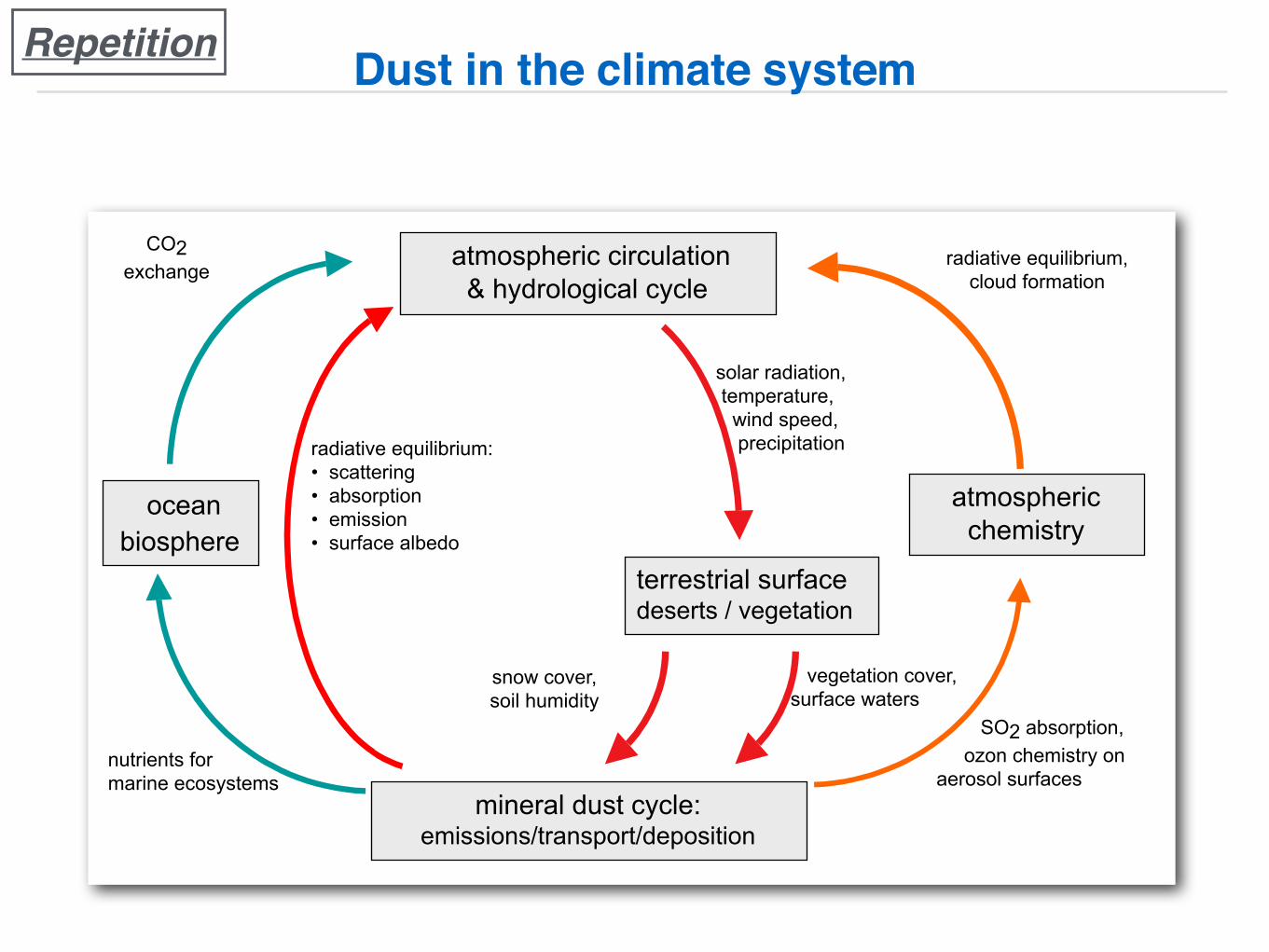
Dust in the climate system
atmospheric circulation & hydrological cycle
mineral dust cycle: emissions/transport/deposition
radiative equilibrium: • scattering • absorption • emission • surface albedo
snow cover, soil humidity
terrestrial surface deserts / vegetation
vegetation cover, surface waters
solar radiation, temperature, wind speed, precipitation
ocean biosphere
nutrients for marine ecosystems
CO2 exchange
atmospheric chemistry
radiative equilibrium, cloud formation
SO2 absorption, ozon chemistry on aerosol surfaces
Repetition
RepetitionLGM dust cycle: fertilisation of the marine biosphere
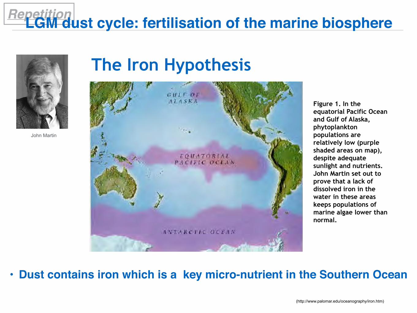
The Iron Hypothesis
John Martin
Figure 1. In the equatorial Pacific Ocean and Gulf of Alaska, phytoplankton populations are relatively low (purple shaded areas on map), despite adequate sunlight and nutrients. John Martin set out to prove that a lack of dissolved iron in the water in these areas keeps populations of marine algae lower than normal.
(http://www.palomar.edu/oceanography/iron.htm)
• Dust contains iron which is a key micro-nutrient in the Southern Ocean
RepetitionLGM dust cycle: fertilisation of the marine biosphere
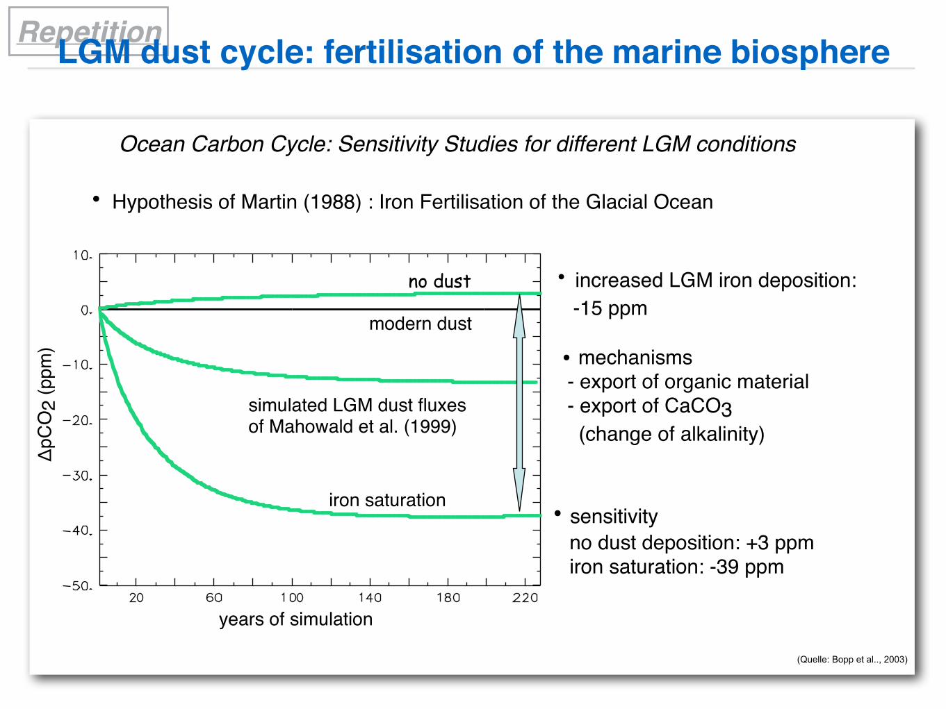
(Quelle: Bopp et al.., 2003)
Ocean Carbon Cycle: Sensitivity Studies for different LGM conditions
• Hypothesis of Martin (1988) : Iron Fertilisation of the Glacial Ocean
years of simulation
ΔpC
O2
(ppm
)
• increased LGM iron deposition: -15 ppm
simulated LGM dust fluxes of Mahowald et al. (1999)
• mechanisms - export of organic material - export of CaCO3 (change of alkalinity)
• sensitivity no dust deposition: +3 ppm iron saturation: -39 ppm
iron saturation
no dust
modern dust
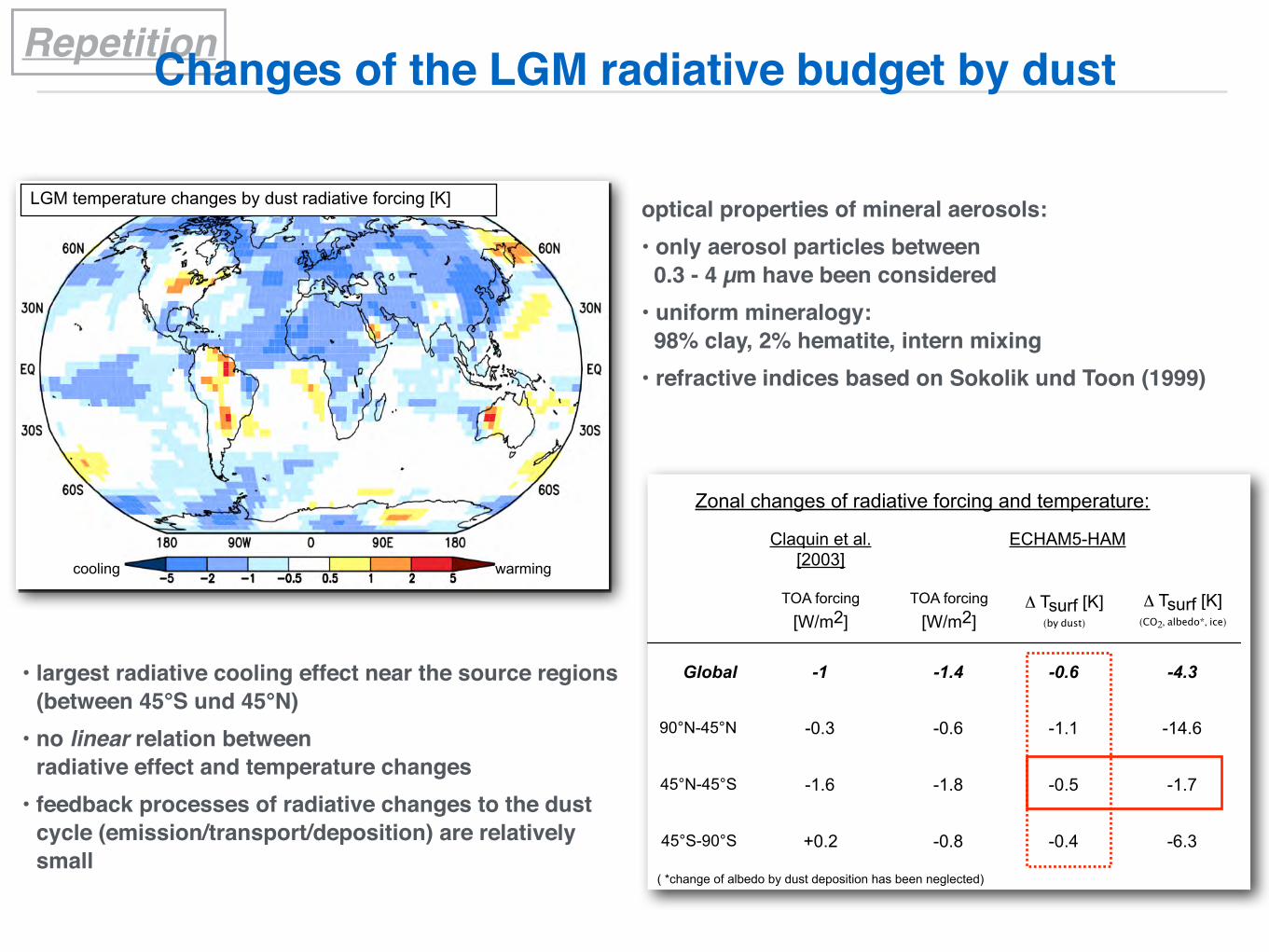
RepetitionChanges of the LGM radiative budget by dust
LGM temperature changes by dust radiative forcing [K]
cooling warming
• largest radiative cooling effect near the source regions (between 45°S und 45°N)
• no linear relation between radiative effect and temperature changes
• feedback processes of radiative changes to the dust cycle (emission/transport/deposition) are relatively small
Zonal changes of radiative forcing and temperature:
( *change of albedo by dust deposition has been neglected)
Claquin et al. [2003]
ECHAM5-HAM
TOA forcing
[W/m2]TOA forcing
[W/m2]Δ Tsurf [K]
(by dust)
Δ Tsurf [K] (CO2, albedo*, ice)
Global -1 -1.4 -0.6 -4.3
90°N-45°N -0.3 -0.6 -1.1 -14.6
45°N-45°S -1.6 -1.8 -0.5 -1.7
45°S-90°S +0.2 -0.8 -0.4 -6.3
optical properties of mineral aerosols:• only aerosol particles between 0.3 - 4 µm have been considered
• uniform mineralogy:98% clay, 2% hematite, intern mixing
• refractive indices based on Sokolik und Toon (1999)
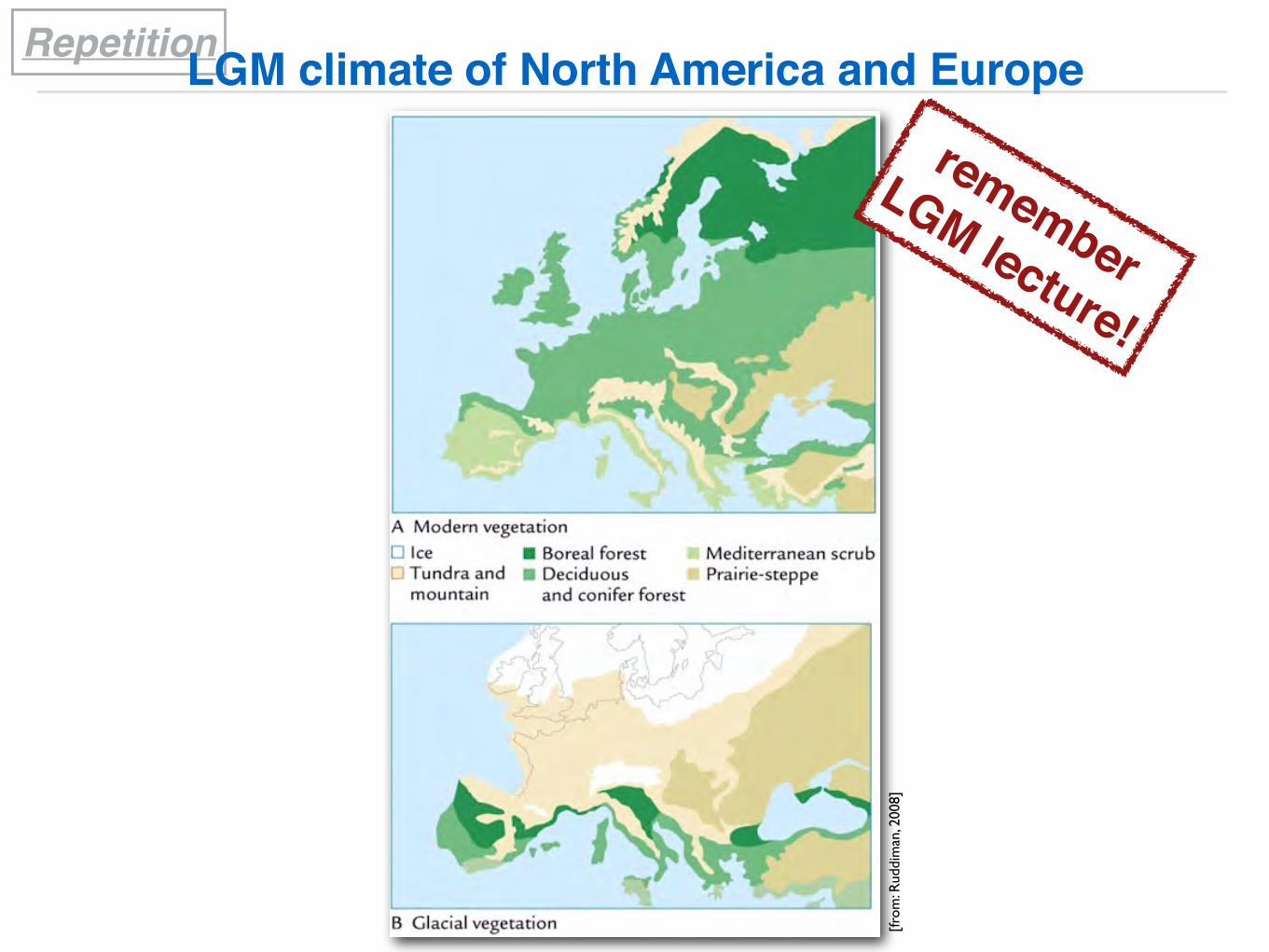
RepetitionLGM climate of North America and Europe
[fro
m: R
uddi
man
, 200
8]
remember LGM lecture!

RepetitionModern and LGM dust deposition fluxes
simulation: ECHAM-4 GCM climatology (modern and LGM, respectively) reconstructions: DIRTMAP Datenbank
(DIRTMAP: Dust Indicator and Records of Terrestrial and Marine Paleoenvironments)
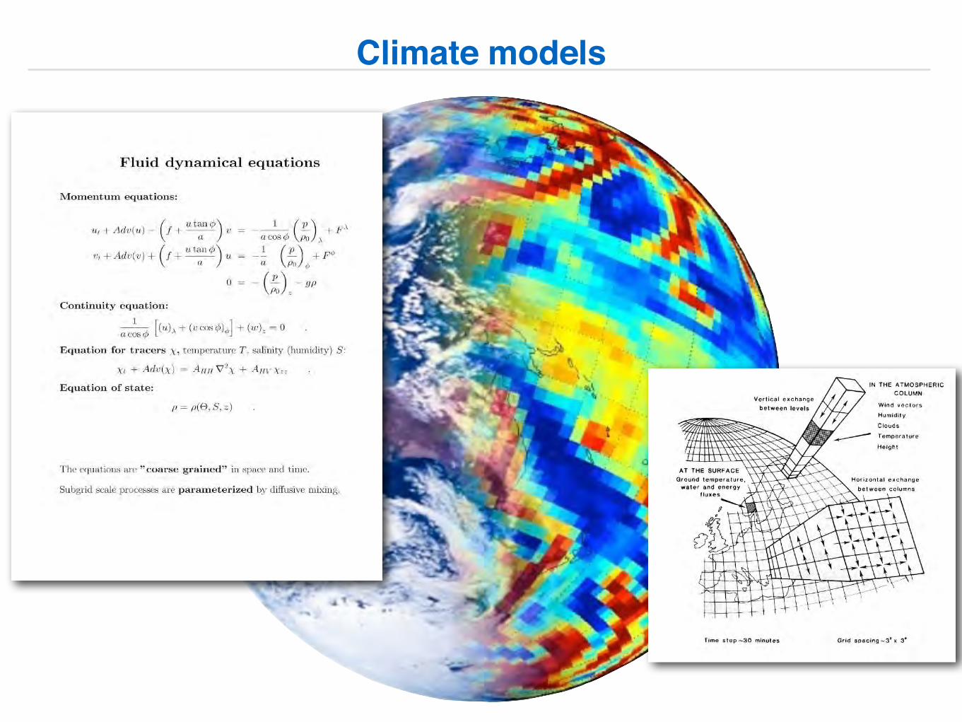
Climate models
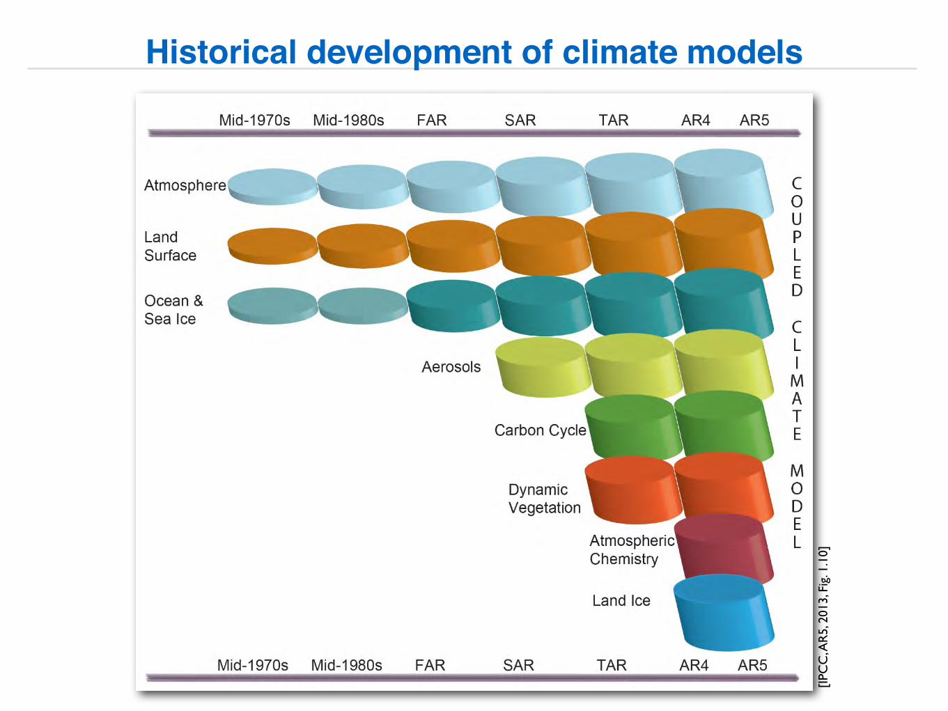
Historical development of climate models
[IPC
C, A
R5,
201
3, F
ig. 1
.10]
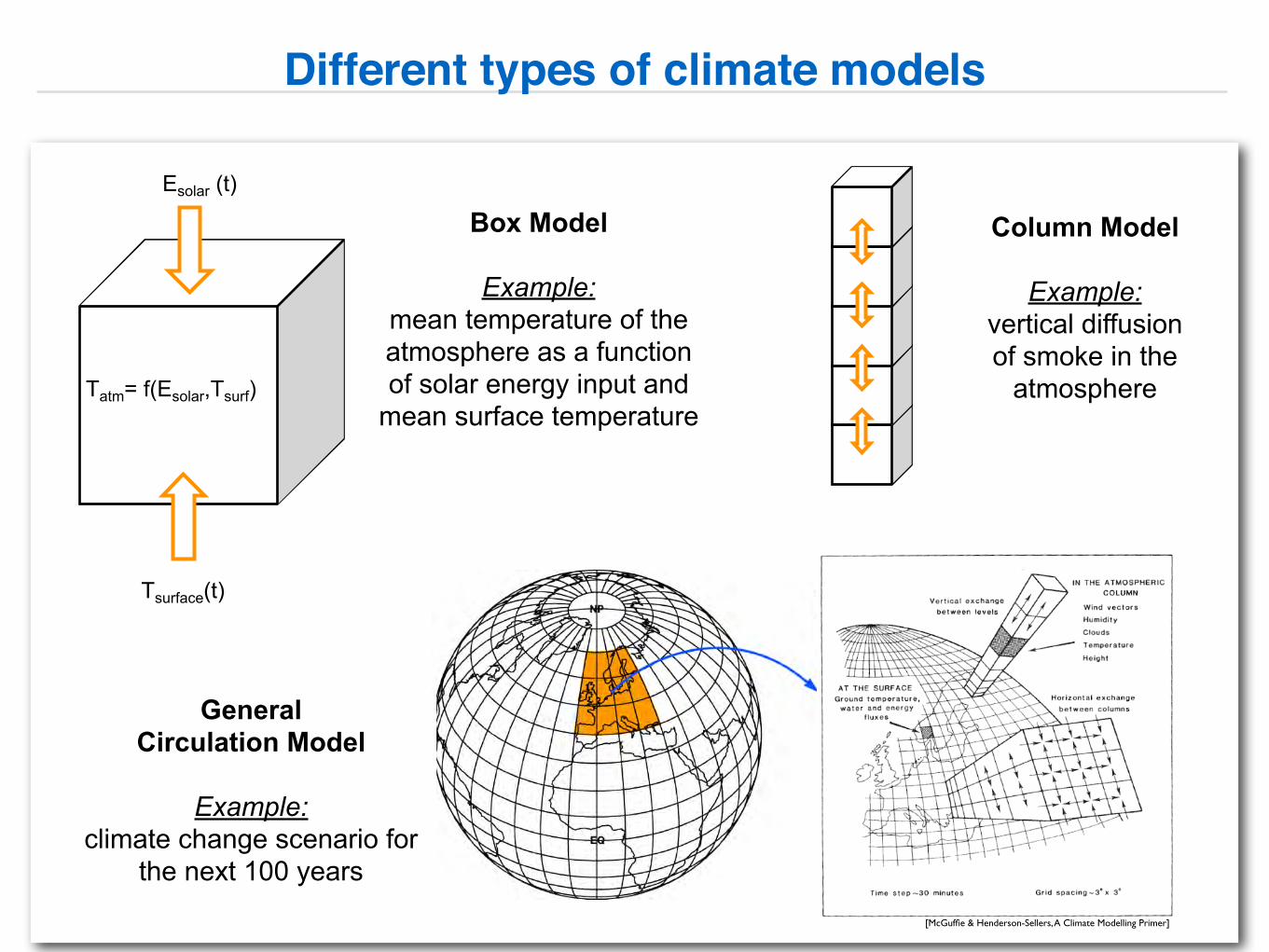
Box Model
Example: mean temperature of the atmosphere as a function of solar energy input and
mean surface temperature
General Circulation Model
Example: climate change scenario for
the next 100 years
Column Model
Example: vertical diffusion of smoke in the
atmosphere
Esolar (t)
Tsurface(t)
Tatm= f(Esolar,Tsurf)
Different types of climate models
[McGuffie & Henderson-Sellers, A Climate Modelling Primer]
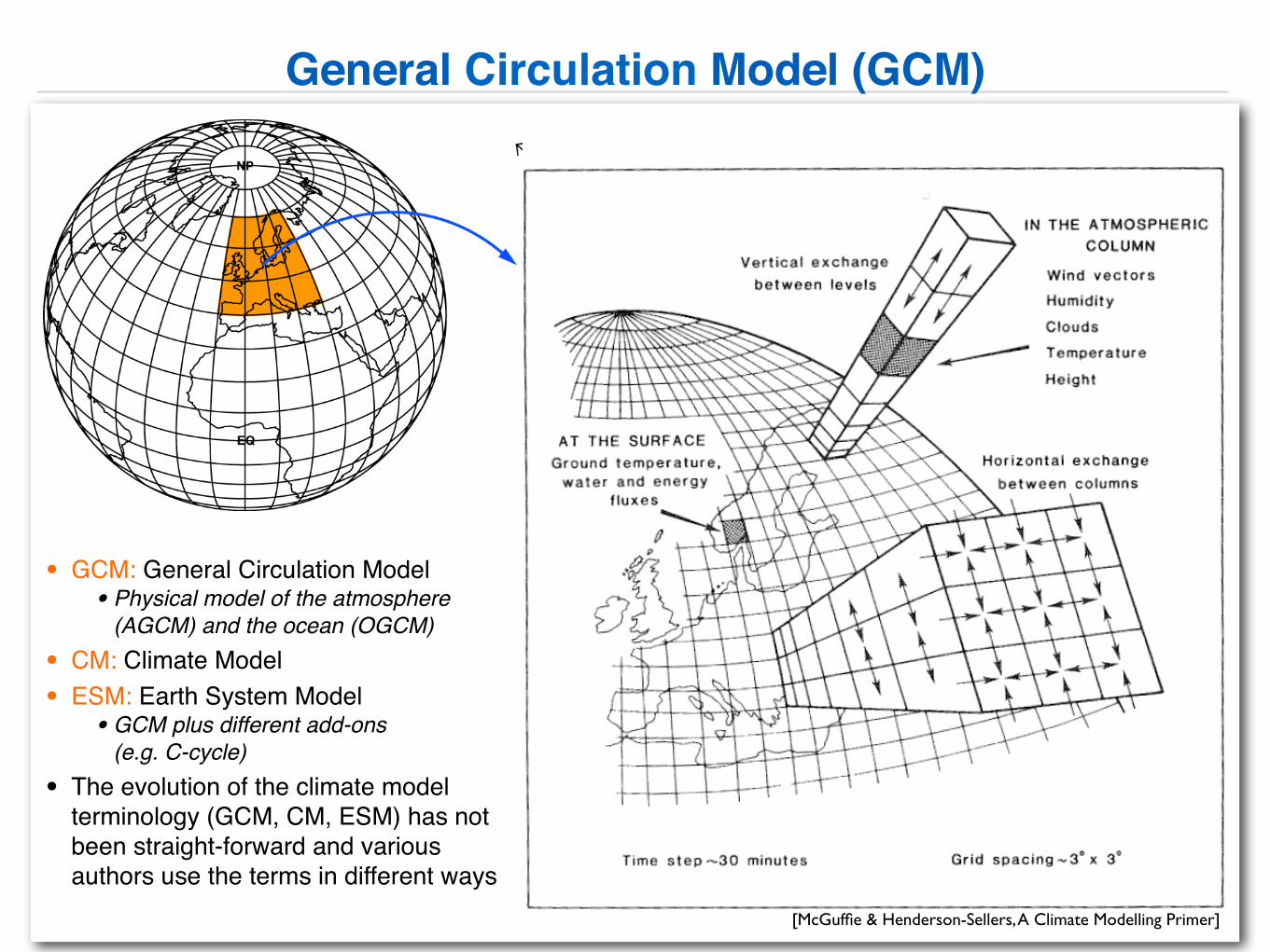
General Circulation Model (GCM)
• GCM: General Circulation Model• Physical model of the atmosphere
(AGCM) and the ocean (OGCM)
• CM: Climate Model• ESM: Earth System Model
• GCM plus different add-ons (e.g. C-cycle)
• The evolution of the climate model terminology (GCM, CM, ESM) has not been straight-forward and various authors use the terms in different ways
[McGuffie & Henderson-Sellers, A Climate Modelling Primer]
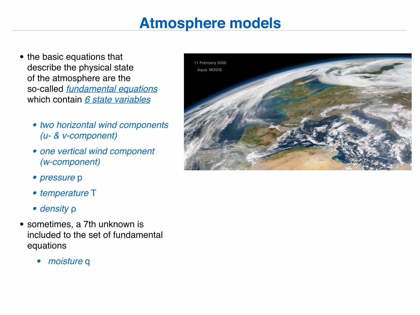
Atmosphere models
• the basic equations that describe the physical state of the atmosphere are the so-called fundamental equationswhich contain 6 state variables
• two horizontal wind components(u- & v-component)
• one vertical wind component (w-component)
• pressure p
• temperature T
• density ρ
• sometimes, a 7th unknown is included to the set of fundamental equations
• moisture q
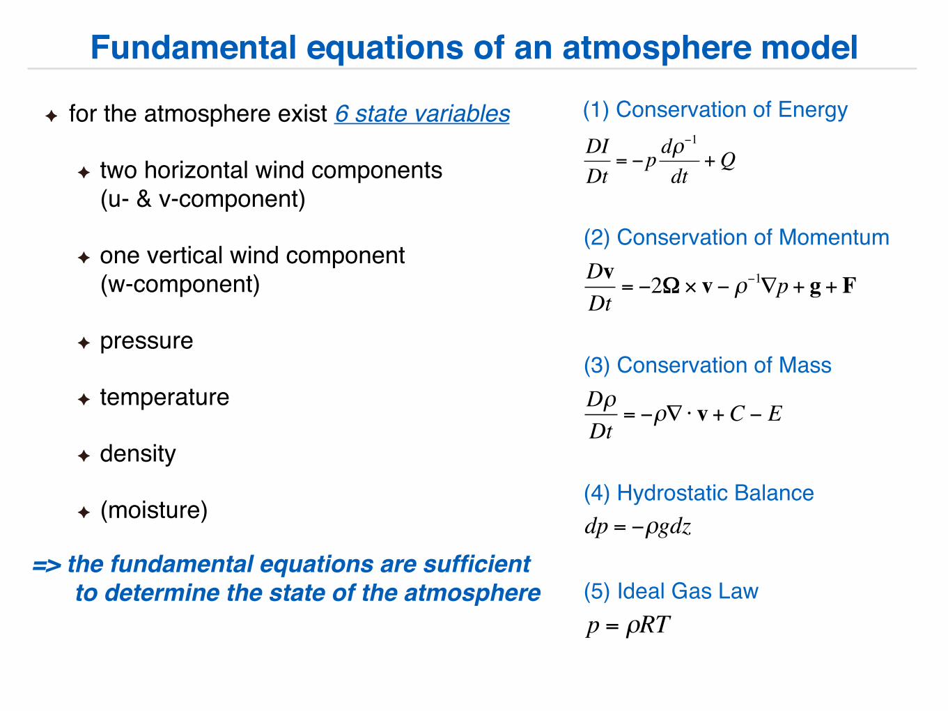
Fundamental equations of an atmosphere model
for the atmosphere exist 6 state variables
two horizontal wind components (u- & v-component)
one vertical wind component (w-component)
pressure
temperature
density
(moisture)
=> the fundamental equations are sufficient to determine the state of the atmosphere
€
DIDt
= −p dρ−1
dt+Q
(1) Conservation of Energy
€
DvDt
= −2Ω× v − ρ−1∇p + g + F
(2) Conservation of Momentum
€
DρDt
= −ρ∇ ⋅ v + C − E
(3) Conservation of Mass
€
dp = −ρgdz(4) Hydrostatic Balance
€
p = ρRT(5) Ideal Gas Law
[McG
uffie
& H
ende
rson
-Sel
lers
, A C
limat
e M
odel
ling
Prim
er, 2
005]
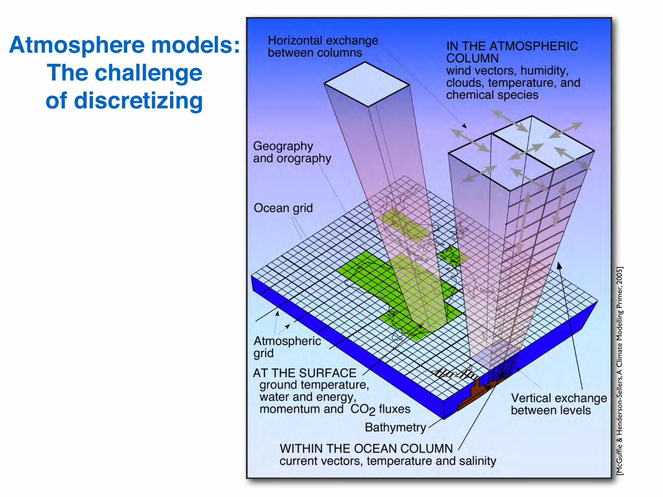
Atmosphere models:The challengeof discretizing
[Trenberth, Climate System Modeling, 1993]
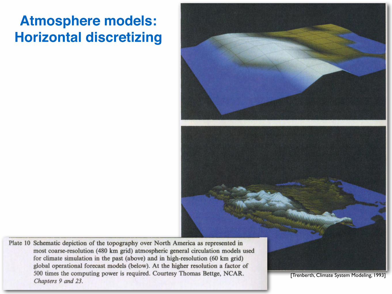
Atmosphere models:Horizontal discretizing
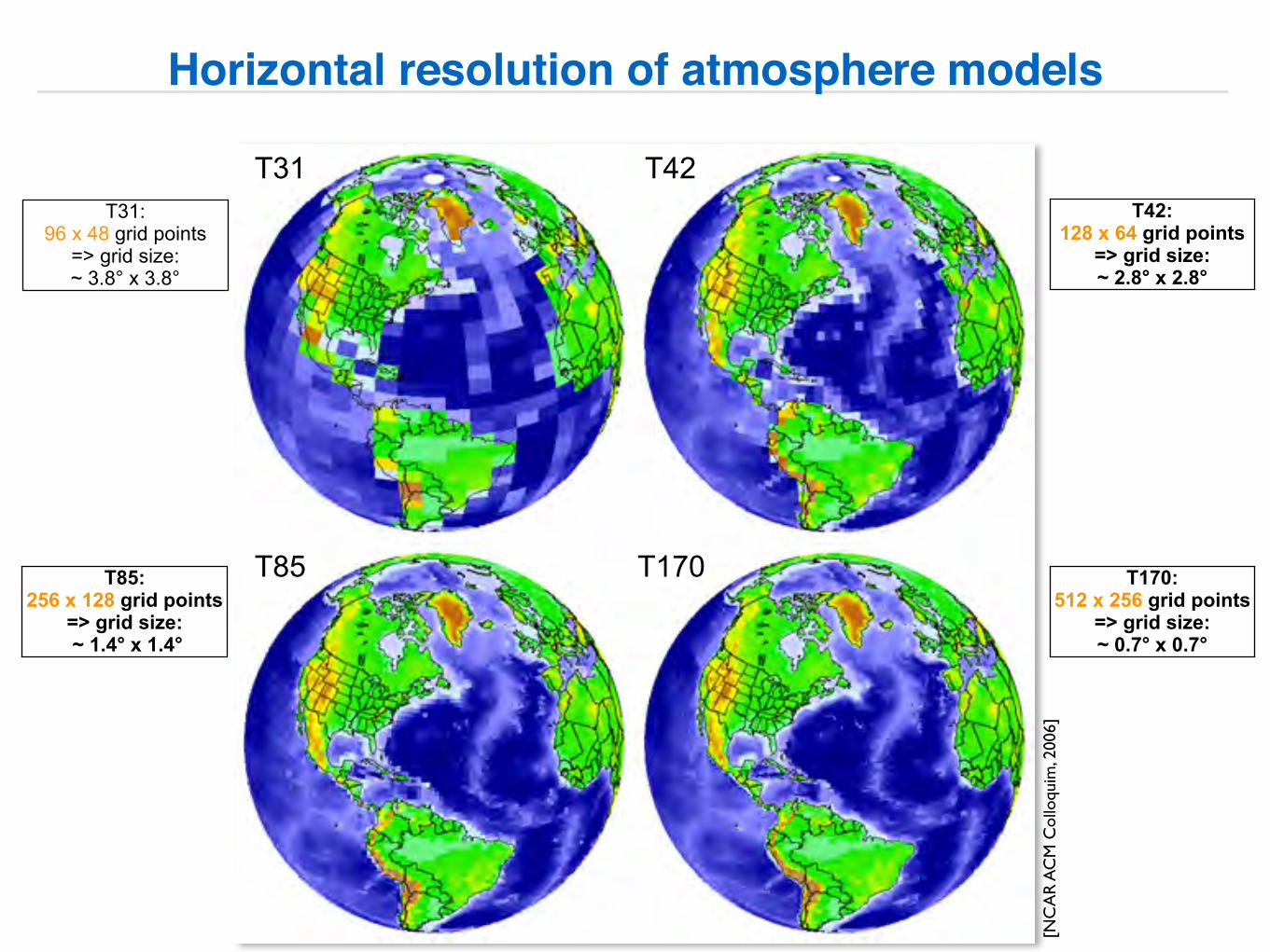
Horizontal resolution of atmosphere models
T31 T42
T85 T170
[NC
AR
AC
M C
ollo
quim
, 200
6]
T31: 96 x 48 grid points
=> grid size: ~ 3.8° x 3.8°
T85: 256 x 128 grid points
=> grid size: ~ 1.4° x 1.4°
T170: 512 x 256 grid points
=> grid size: ~ 0.7° x 0.7°
T42: 128 x 64 grid points
=> grid size: ~ 2.8° x 2.8°

[MPI
Met
eoro
logy
Ham
burg
, The
EC
HA
M3
AG
CM
, Tec
h. R
epor
t N
o. 6
, 199
3]Sigma Coordinate (Simplest Form):
Define new coordinate variable s as
σ = p / psurf
=> at surface: σ = 1 at top of atmosphere: σ = 0
Atmosphere models:Vertical discretizing

Temporal discretizing
• Relation between spatial grid size and model time step:The time step must be short enough that the maximum speed of propagation of information does not permit any transfer from one grid point to another within one time step
Δt ≤ Δx / c ( c = propagation velocity)
• Example: ECHAM atmosphere GCM
GCM Mode # grid points grid size time step
T21 64 x 32 ~5.6° 40min
T42 128 x 64 ~2.8° 24min
T106 320 x 160 ~1.1° 12min
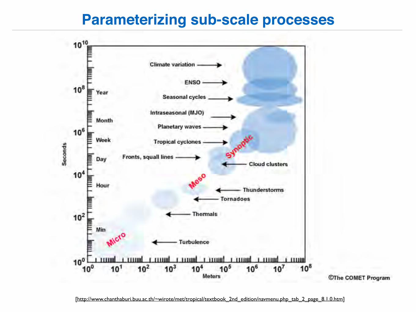
Parameterizing sub-scale processes
[http://www.chanthaburi.buu.ac.th/~wirote/met/tropical/textbook_2nd_edition/navmenu.php_tab_2_page_8.1.0.htm]

Sub-scale processes: Radiation in the atmosphere
[McG
uffie
& H
ende
rson
-Sel
lers
, A C
limat
e M
odel
ling
Prim
er, 2
005]
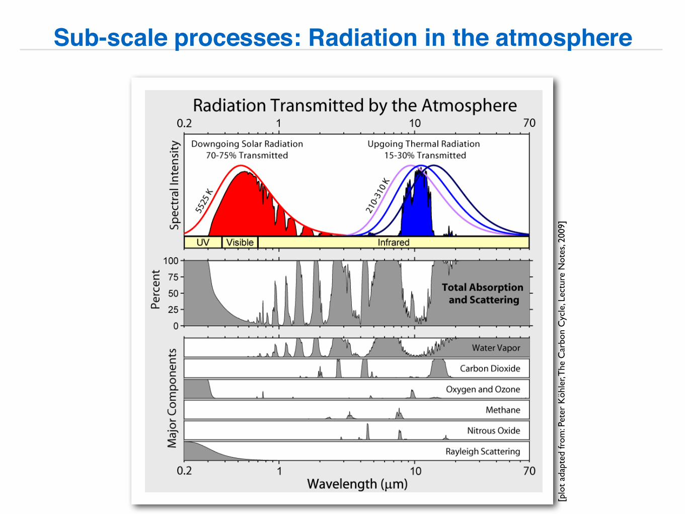
Sub-scale processes: Radiation in the atmosphere
Forcing
Atmospheric Spectral Transmission
Earth: 4� 100µm
�max = 11µm (IR)
H2O: Absorption 5� 8µm; > 17µm
CO2: Absorption 13� 17µm
Transmission window : 8� 13µm
Peter Köhler (AWI Bremerhaven) 02 — Radiative Forcing of GHG and Future 03/11/2009, Uni HB 19 / 57
[plo
t ad
apte
d fr
om: P
eter
Köh
ler, T
he C
arbo
n C
ycle
, Lec
ture
Not
es, 2
009]
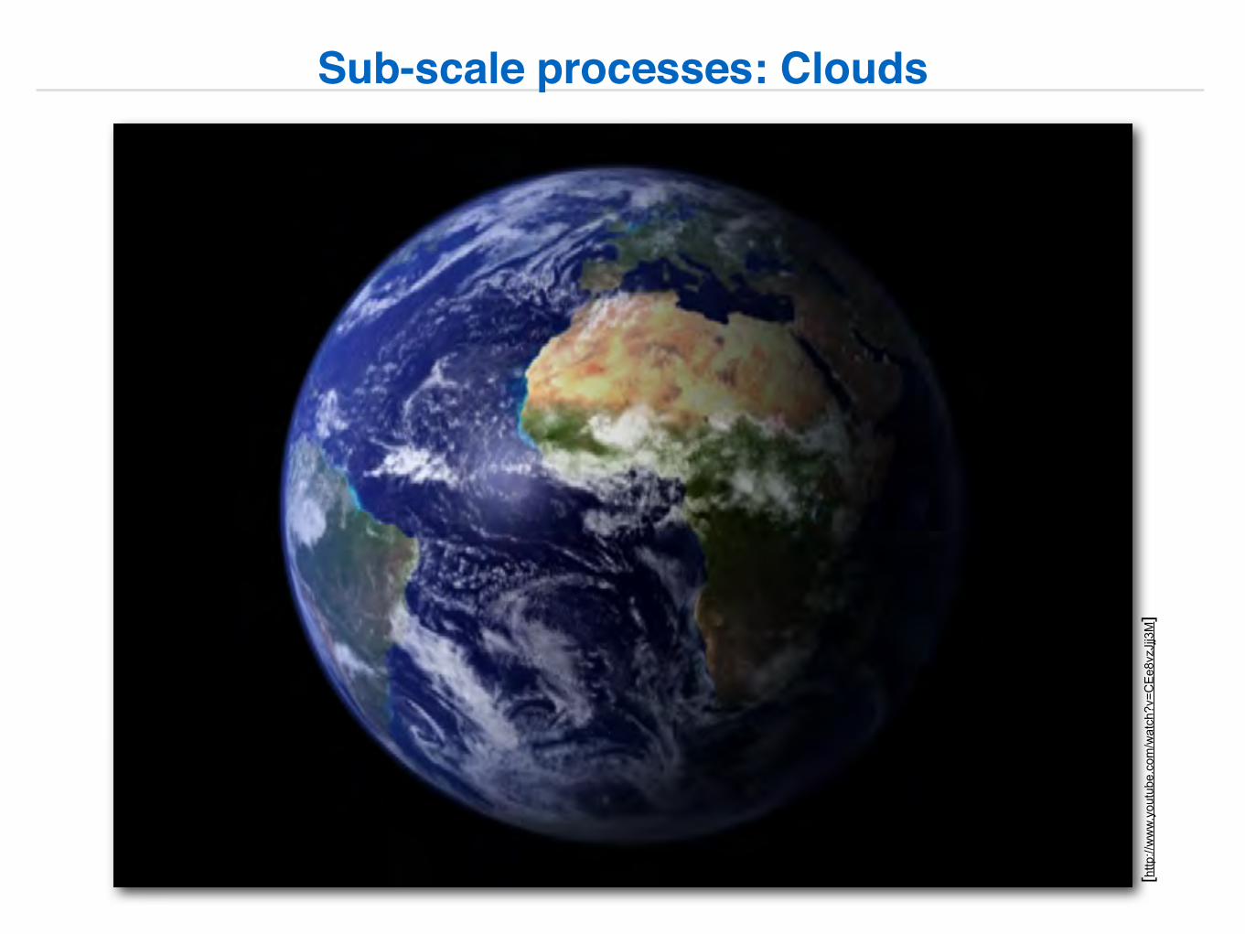
Sub-scale processes: Clouds
[http
://w
ww
.you
tube
.com
/wat
ch?v
=CE
e8vz
Jjj3
M]
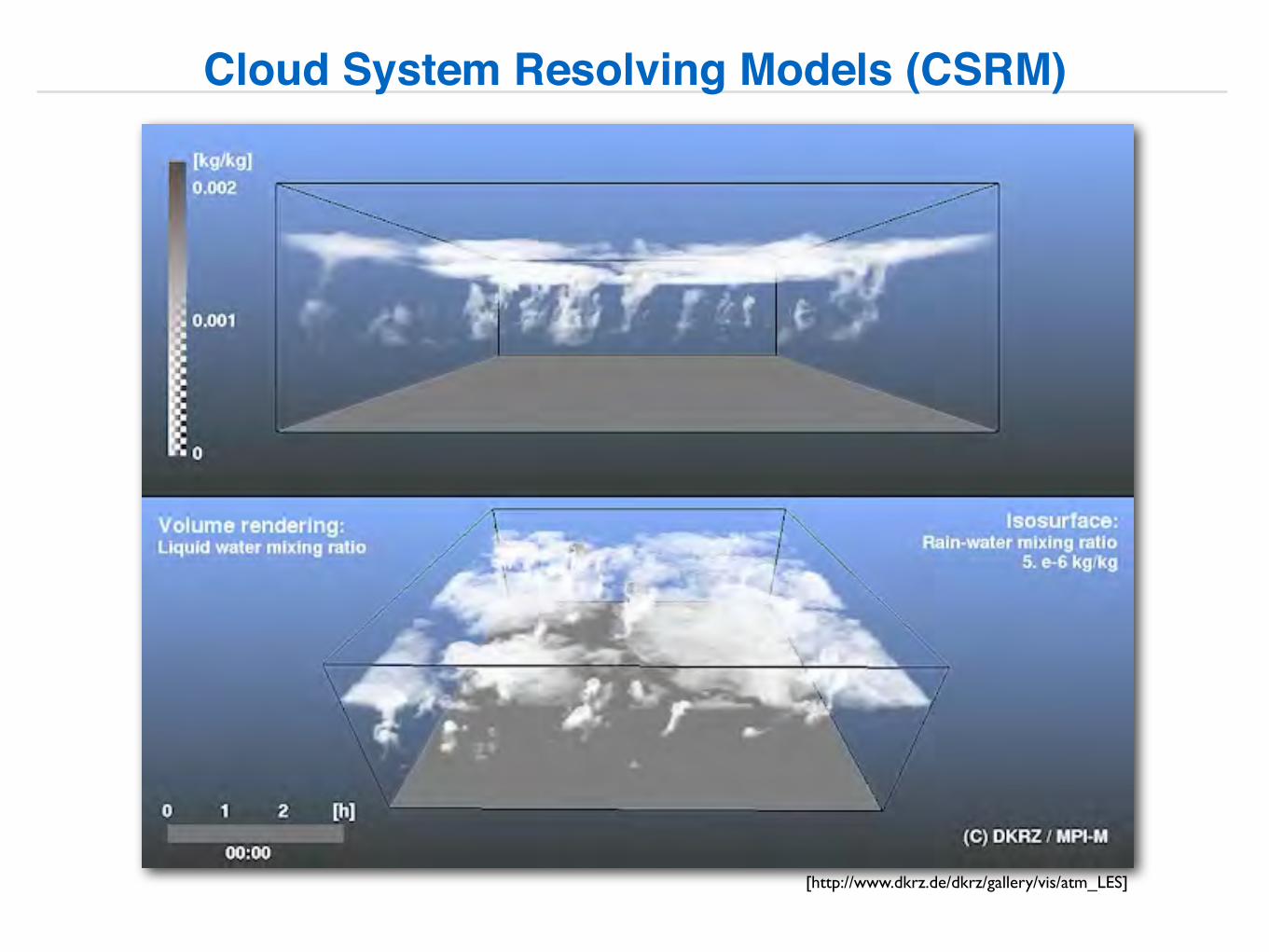
Cloud System Resolving Models (CSRM)
[http://www.dkrz.de/dkrz/gallery/vis/atm_LES]
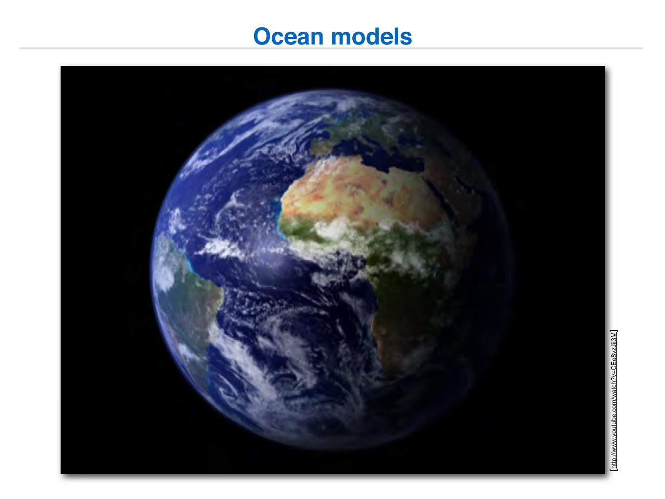
Ocean models
[http
://w
ww
.you
tube
.com
/wat
ch?v
=CE
e8vz
Jjj3
M]
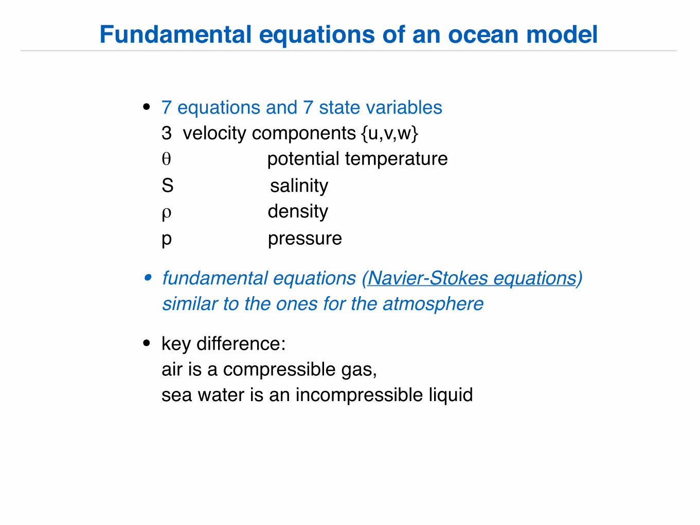
• 7 equations and 7 state variables3 velocity components {u,v,w}θ potential temperatureS salinityρ densityp pressure
• fundamental equations (Navier-Stokes equations) similar to the ones for the atmosphere
• key difference: air is a compressible gas, sea water is an incompressible liquid
Fundamental equations of an ocean model
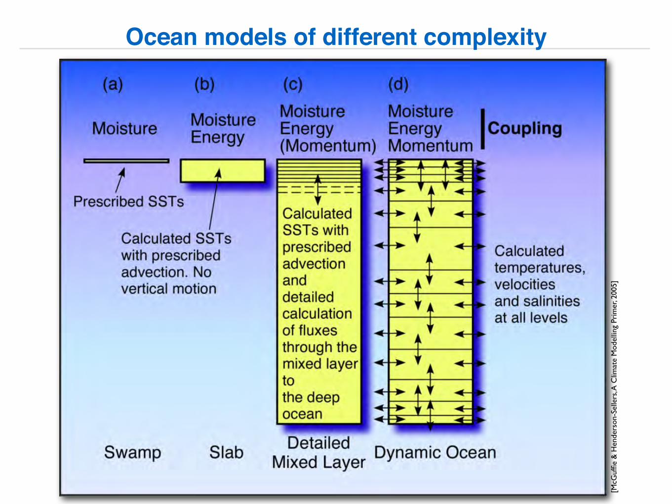
Ocean models of different complexity
[McG
uffie
& H
ende
rson
-Sel
lers
, A C
limat
e M
odel
ling
Prim
er, 2
005]
Ocean grids
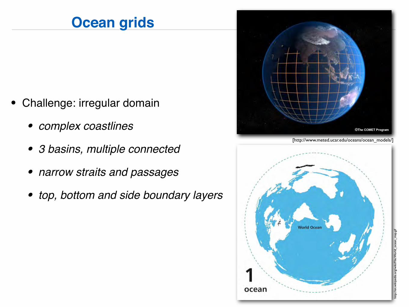
• Challenge: irregular domain
• complex coastlines
• 3 basins, multiple connected
• narrow straits and passages
• top, bottom and side boundary layers
[http://www.meted.ucar.edu/oceans/ocean_models/]
http
://en
.wik
iped
ia.o
rg/w
iki/F
ile:W
orld
_oce
an_m
ap.g
if
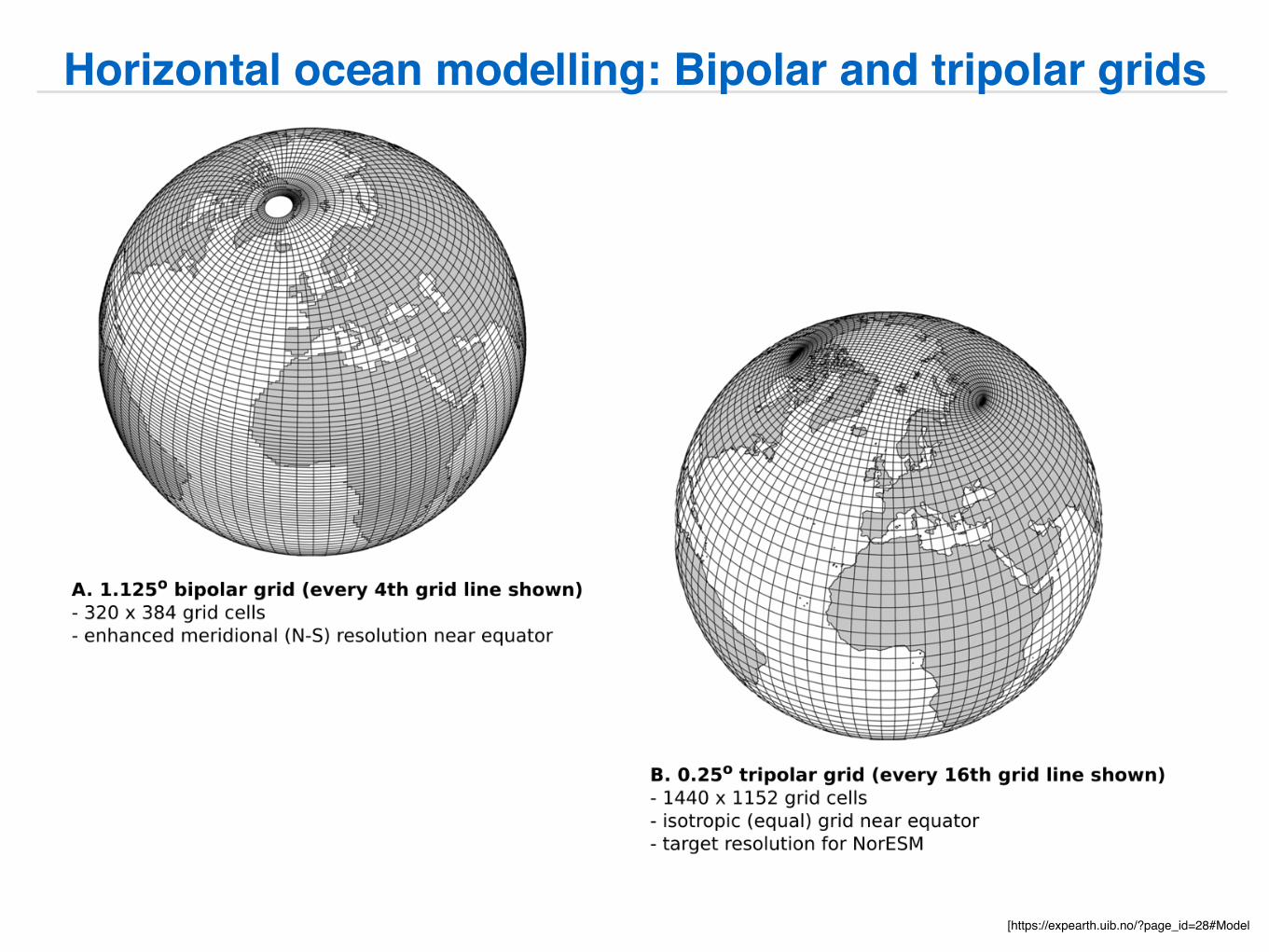
Horizontal ocean modelling: Bipolar and tripolar grids
[https://expearth.uib.no/?page_id=28#Model

Horizontal ocean modelling: Finite Elements
[https://fesom.de/models/awi-esm/]

Vertical ocean model grids
[htt
p://w
ww
.met
ed.u
car.e
du/o
cean
s/oc
ean_
mod
els/
]
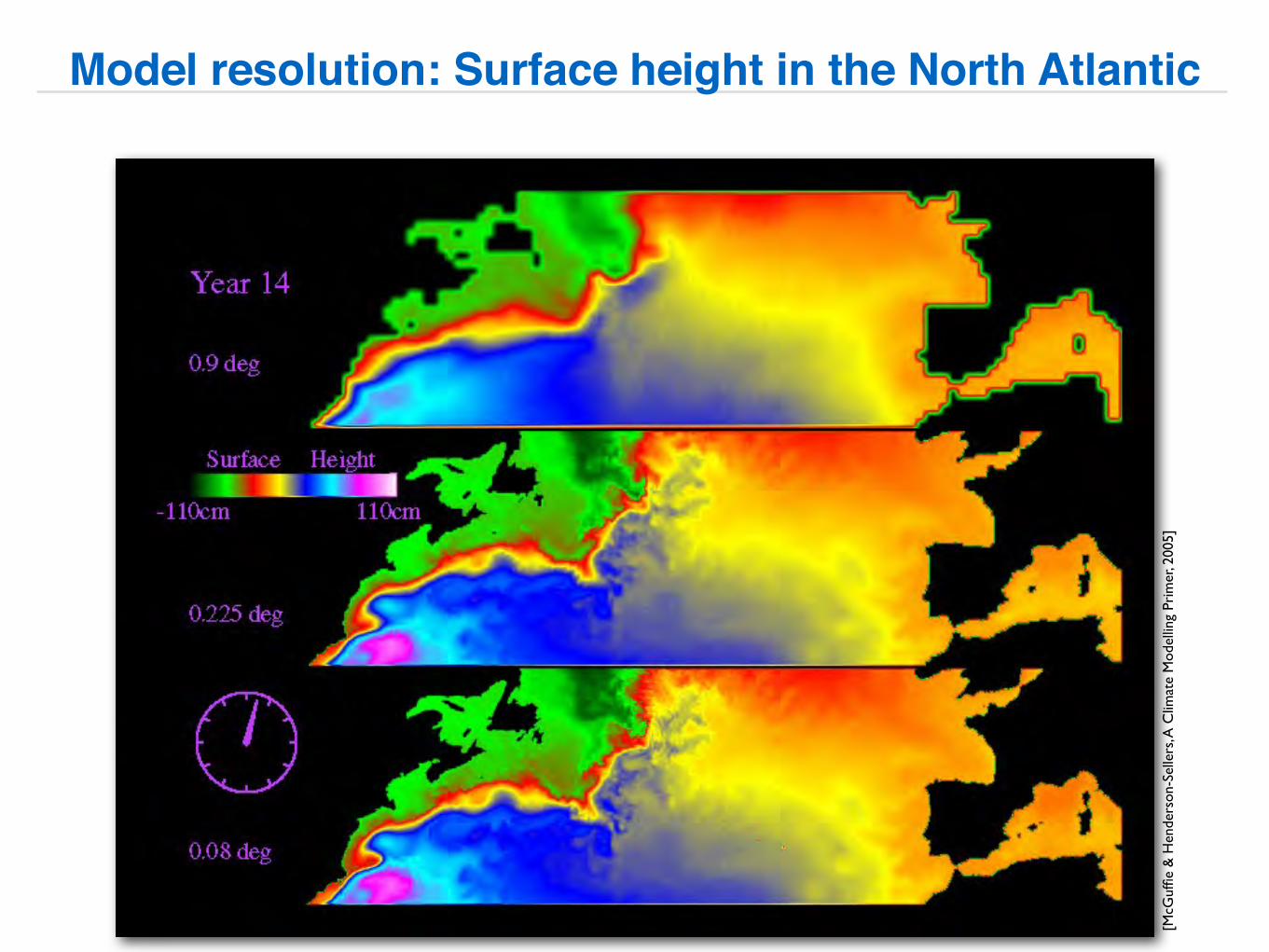
Model resolution: Surface height in the North Atlantic
[McG
uffie
& H
ende
rson
-Sel
lers
, A C
limat
e M
odel
ling
Prim
er, 2
005]

Coupling of atmosphere and ocean GCM
[McGuffie & Henderson-Sellers, A Climate Modelling Primer, 2005]
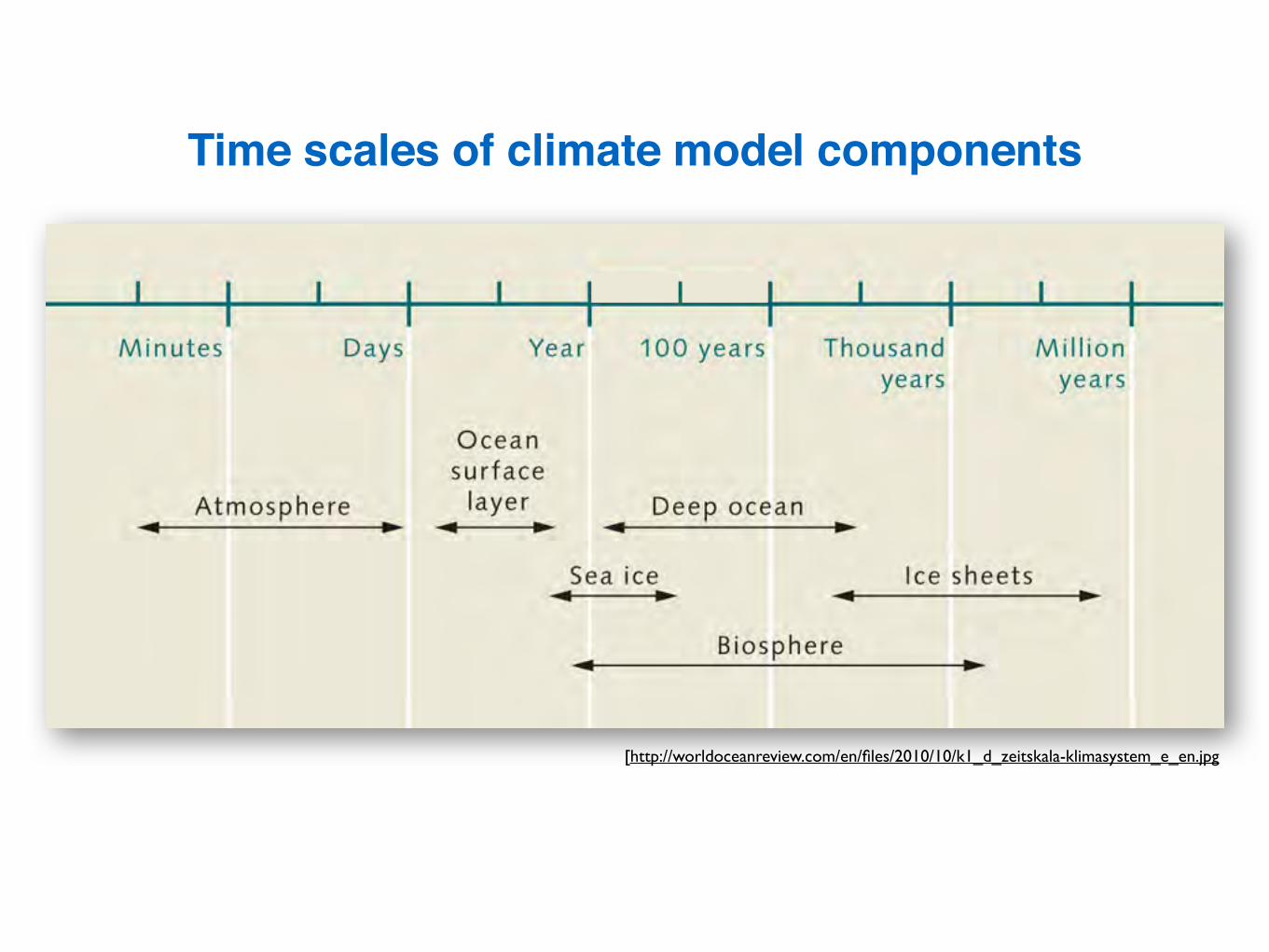
[http://worldoceanreview.com/en/files/2010/10/k1_d_zeitskala-klimasystem_e_en.jpg
Time scales of climate model components
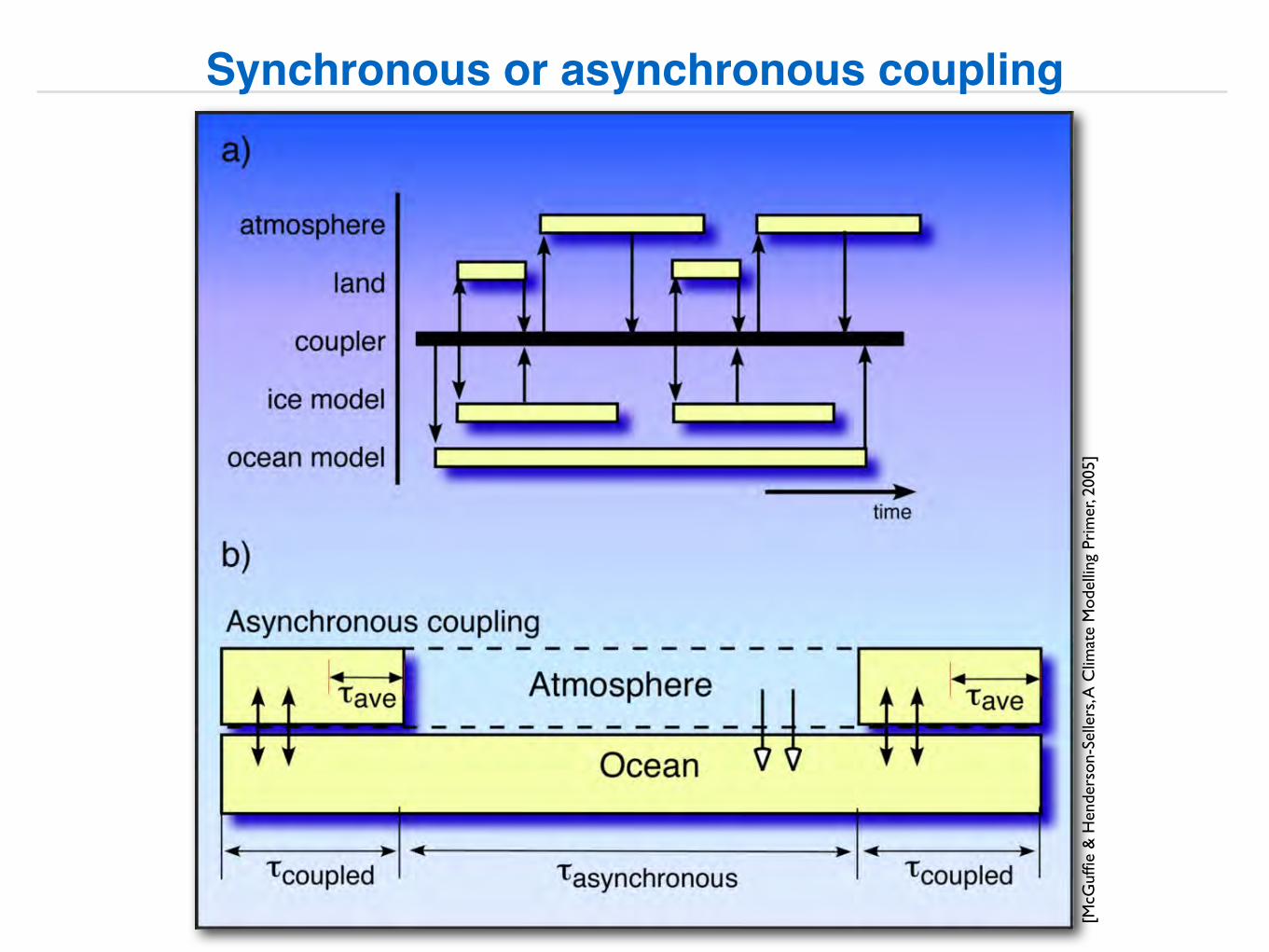
Synchronous or asynchronous coupling
[McG
uffie
& H
ende
rson
-Sel
lers
, A C
limat
e M
odel
ling
Prim
er, 2
005]

[McGuffie & Henderson-Sellers, A Climate Modelling Primer]
Model challenges:Complexity of interaction between different physical processes...

[MPI
Met
eoro
logy
Ham
burg
, The
EC
HA
M3
AG
CM
, Tec
h. R
epor
t N
o. 6
, 199
3]
Model challenges:Complexity of interaction between different physical processes...

(Re-)Initialization (e.g. SST,
Vegetation Coverage)
Grid Scan #1
Grid Scan #2
Soil Processes
Vertical Diffusion
Convection
Large Scale Condensation
Radiation
Output of Data Field
Statistical Output
Exchange (Advection & Diffusion)
Between Different Grid Boxes
Start
Stop
Loop
ove
r Tim
e S
teps
Loop over Longitude & Latitude
Loop over Longitude &
Latitude &
Vertical LevelsLoop over Vertical Levels
Example: An atmosphere GCM flow diagram

grid cell
glacier wetland lake
land units
vertical columns
plant functionaltypes (PFT)
urbanvegetated
soil type 1
Land surface models
[ada
pted
from
: htt
p://w
ww
.asp
.uca
r.edu
/col
loqu
ium
/200
6/cl
imat
e-m
odel
/]
soil type 2soil type 3
crops trees shrubstundra
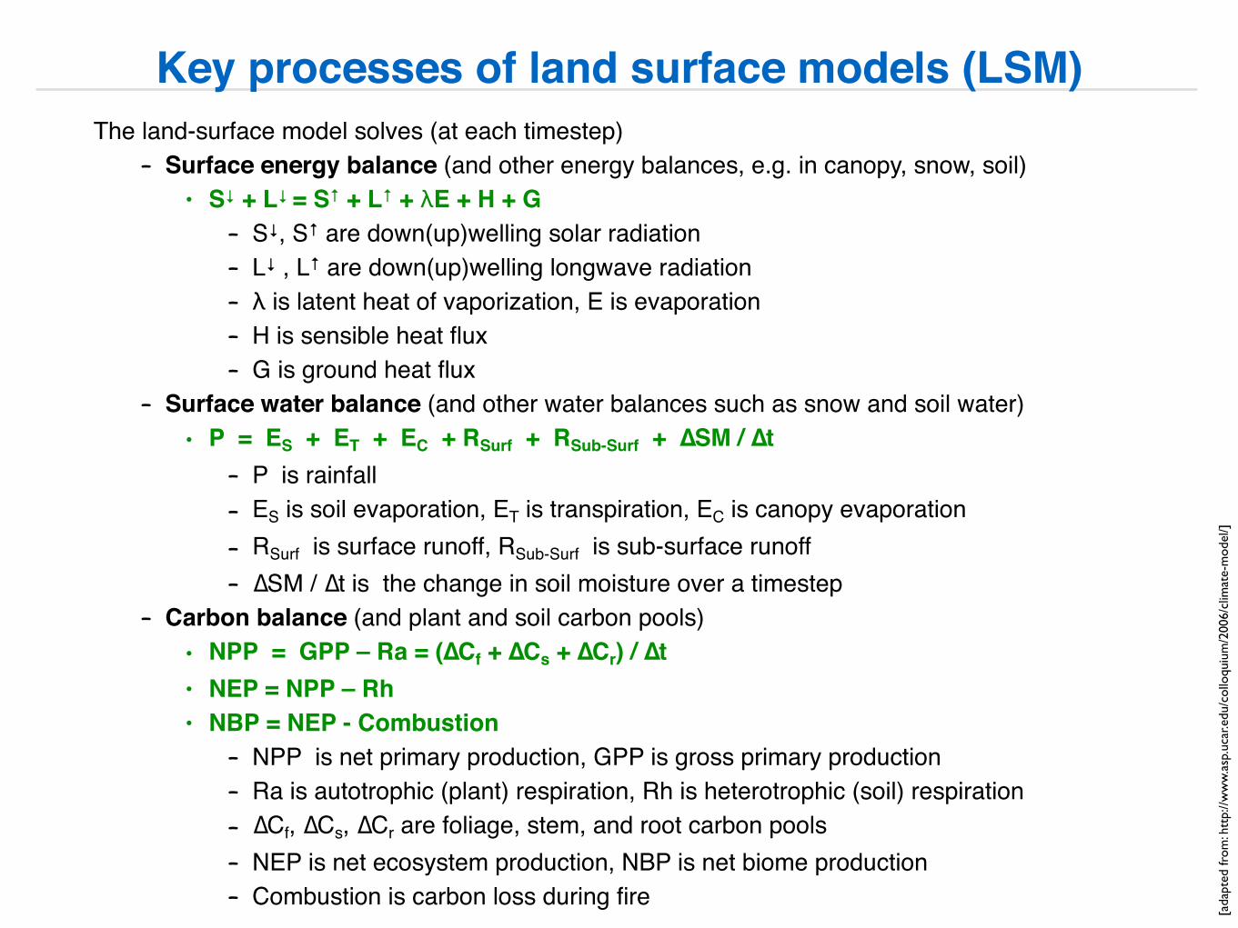
The land-surface model solves (at each timestep)– Surface energy balance (and other energy balances, e.g. in canopy, snow, soil)
• S↓ + L↓ = S↑ + L↑ + λE + H + G – S↓, S↑ are down(up)welling solar radiation – L↓ , L↑ are down(up)welling longwave radiation– λ is latent heat of vaporization, E is evaporation– H is sensible heat flux– G is ground heat flux
– Surface water balance (and other water balances such as snow and soil water)• P = ES + ET + EC + RSurf + RSub-Surf + ∆SM / ∆t
– P is rainfall– ES is soil evaporation, ET is transpiration, EC is canopy evaporation– RSurf is surface runoff, RSub-Surf is sub-surface runoff– ∆SM / ∆t is the change in soil moisture over a timestep
– Carbon balance (and plant and soil carbon pools)• NPP = GPP – Ra = (∆Cf + ∆Cs + ∆Cr) / ∆t• NEP = NPP – Rh • NBP = NEP - Combustion
– NPP is net primary production, GPP is gross primary production– Ra is autotrophic (plant) respiration, Rh is heterotrophic (soil) respiration– ∆Cf, ∆Cs, ∆Cr are foliage, stem, and root carbon pools– NEP is net ecosystem production, NBP is net biome production– Combustion is carbon loss during fire
Key processes of land surface models (LSM)
[ada
pted
from
: htt
p://w
ww
.asp
.uca
r.edu
/col
loqu
ium
/200
6/cl
imat
e-m
odel
/]
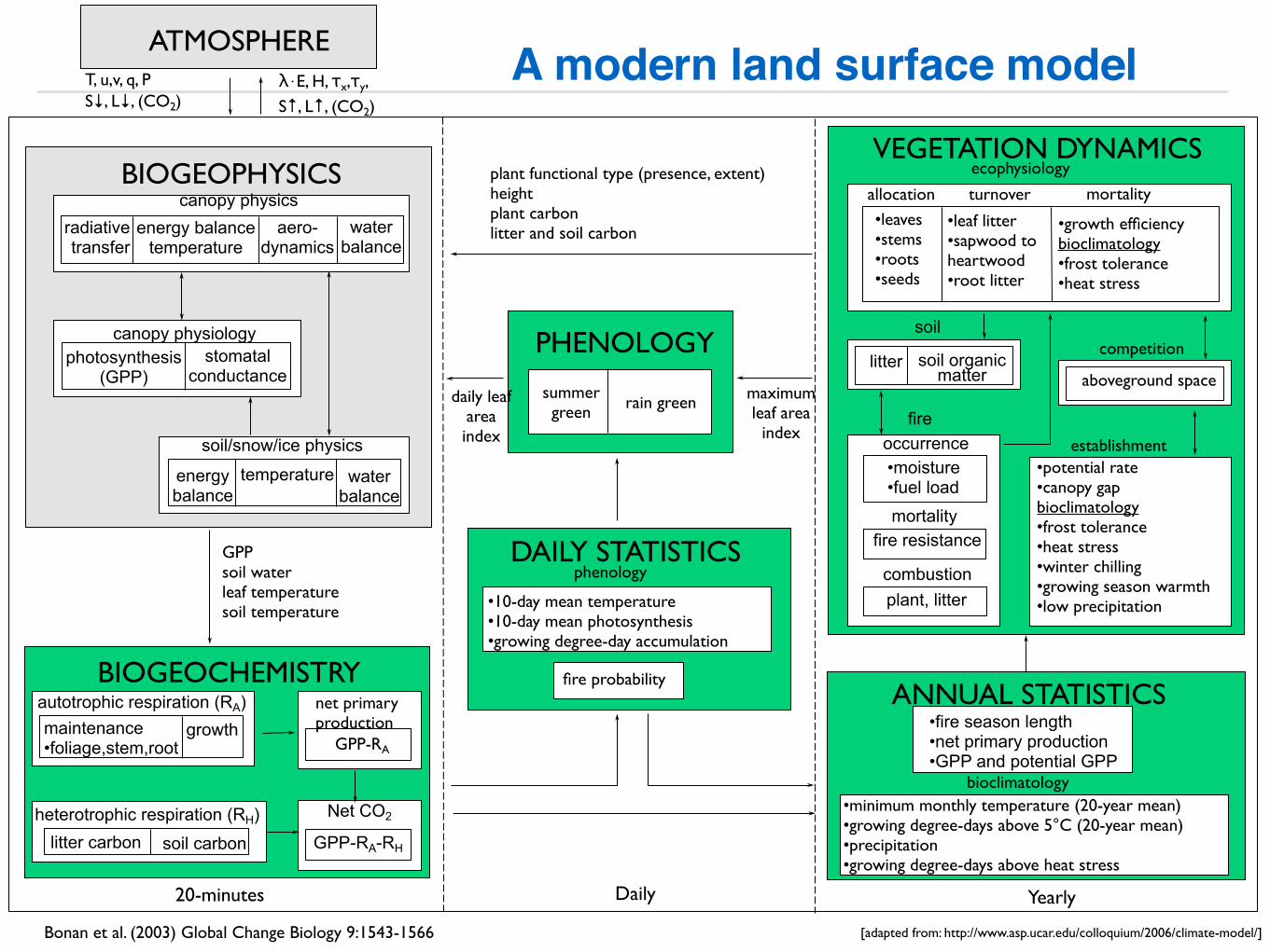
A modern land surface model
BIOGEOPHYSICS
20-minutes YearlyDaily
VEGETATION DYNAMICS
summergreen rain green
PHENOLOGY
daily leaf area index
canopy physiologyphotosynthesis
(GPP)stomatal
conductancemaximum leaf area
index
plant functional type (presence, extent)heightplant carbonlitter and soil carbon
canopy physicsenergy balance
temperaturewater
balanceaero-
dynamicsradiative transfer
T, u,v, q, P S↓, L↓, (CO2)
λ⋅E, H, τx,τy,
S↑, L↑, (CO2)
ATMOSPHERE
soil/snow/ice physics
energy balance
water balance
temperature
BIOGEOCHEMISTRY
heterotrophic respiration (RH)litter carbon soil carbon
autotrophic respiration (RA)maintenance •foliage,stem,root
growthnet primary production
GPP-RA
DAILY STATISTICS
•10-day mean temperature •10-day mean photosynthesis•growing degree-day accumulation
ANNUAL STATISTICS
GPP soil waterleaf temperaturesoil temperature
•leaves•stems•roots•seeds
allocation turnover
•leaf litter•sapwood to heartwood•root litter
mortality
•growth efficiencybioclimatology•frost tolerance•heat stress
ecophysiology
•fire season length •net primary production •GPP and potential GPP
bioclimatology
phenology
fire probability
•potential rate•canopy gapbioclimatology•frost tolerance•heat stress•winter chilling•growing season warmth•low precipitation
establishment
soil organic matter
soil
litteraboveground space
competition
•moisture •fuel load
occurrence
fire resistancemortality
plant, littercombustion
fire
Net CO2
GPP-RA-RH
Bonan et al. (2003) Global Change Biology 9:1543-1566
•minimum monthly temperature (20-year mean)•growing degree-days above 5°C (20-year mean)•precipitation•growing degree-days above heat stress
[adapted from: http://www.asp.ucar.edu/colloquium/2006/climate-model/]
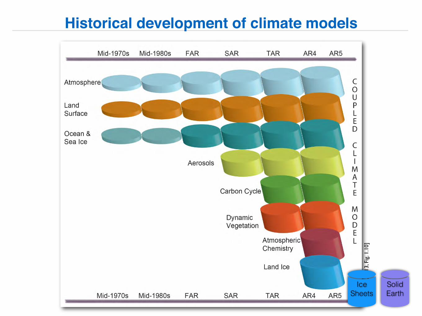
Historical development of climate models
[IPC
C, A
R5,
201
3, F
ig. 1
.10]
Ice Sheets
Solid Earth
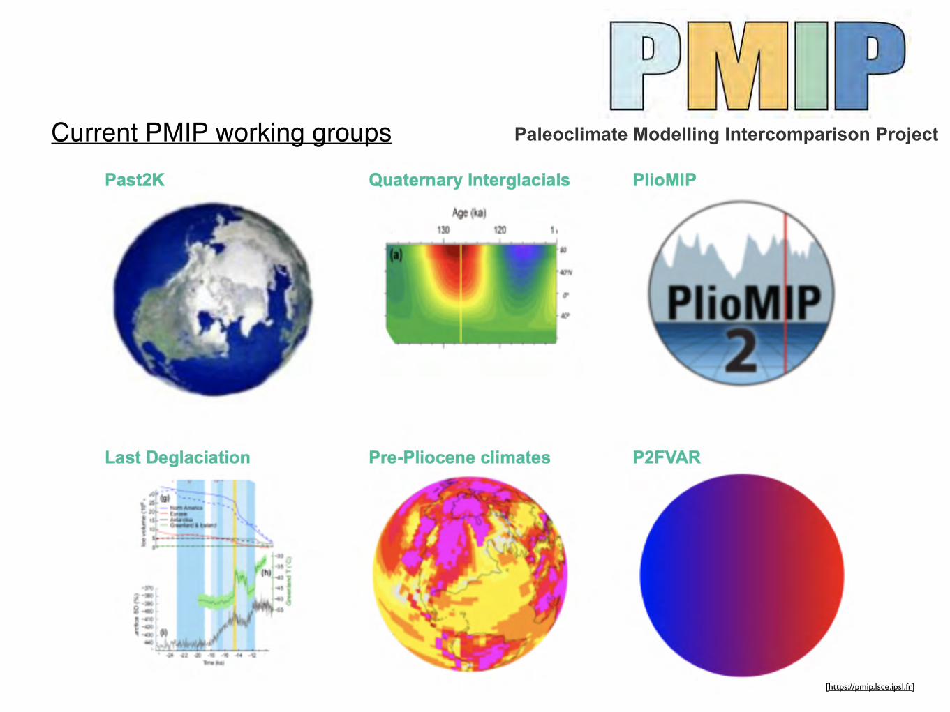
[https://pmip.lsce.ipsl.fr]
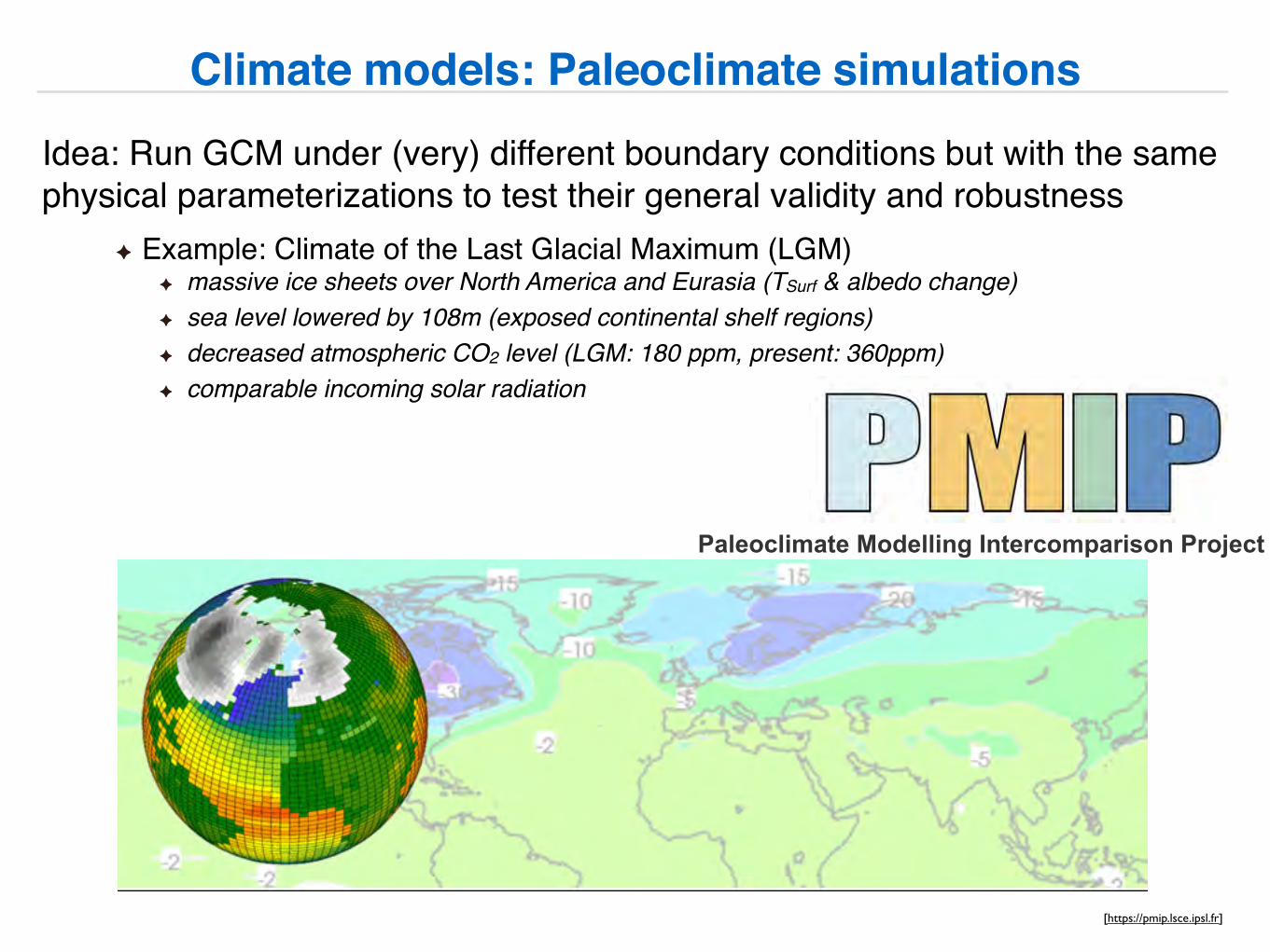
Climate models: Paleoclimate simulationsIdea: Run GCM under (very) different boundary conditions but with the same physical parameterizations to test their general validity and robustness
Example: Climate of the Last Glacial Maximum (LGM)massive ice sheets over North America and Eurasia (TSurf & albedo change)sea level lowered by 108m (exposed continental shelf regions)decreased atmospheric CO2 level (LGM: 180 ppm, present: 360ppm)comparable incoming solar radiation
Paleoclimate Modelling Intercomparison Project
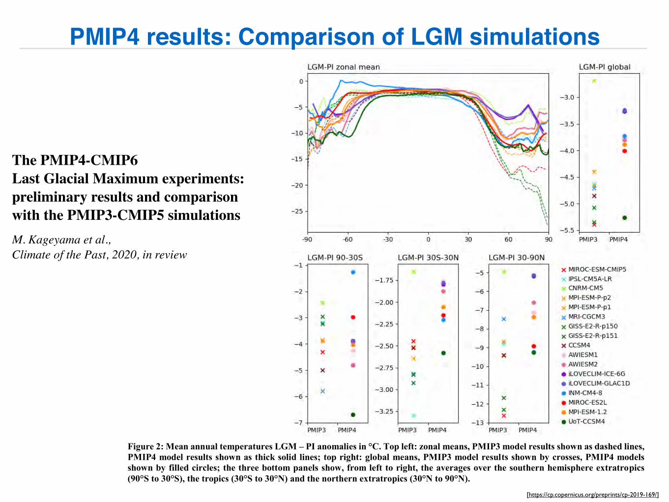
PMIP4 results: Comparison of LGM simulations
[https://cp.copernicus.org/preprints/cp-2019-169/]
Figure 2: Mean annual temperatures LGM – PI anomalies in °C. Top left: zonal means, PMIP3 model results shown as dashed lines, 680 PMIP4 model results shown as thick solid lines; top right: global means, PMIP3 model results shown by crosses, PMIP4 models shown by filled circles; the three bottom panels show, from left to right, the averages over the southern hemisphere extratropics (90°S to 30°S), the tropics (30°S to 30°N) and the northern extratropics (30°N to 90°N).
Page 26 of 37
https://doi.org/10.5194/cp-2019-169Preprint. Discussion started: 23 January 2020c� Author(s) 2020. CC BY 4.0 License.
The PMIP4-CMIP6 Last Glacial Maximum experiments: preliminary results and comparison with the PMIP3-CMIP5 simulationsM. Kageyama et al., Climate of the Past, 2020, in review
[https://pmip.lsce.ipsl.fr]
Paleoclimate Modelling Intercomparison ProjectCurrent PMIP working groups

Climate models: The present climate
[IPCC, AR5, 2013, Fig. FAQ10.1-1]
observations
models (IPCC AR4)models (IPCC AR5)
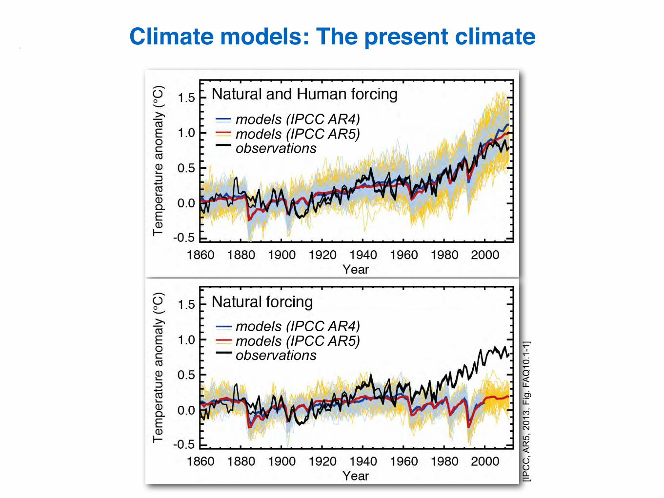
Climate models: The present climate
[IPC
C, A
R5,
201
3, F
ig. F
AQ
10.1
-1]
observations
models (IPCC AR4)models (IPCC AR5)
observations
models (IPCC AR4)models (IPCC AR5)
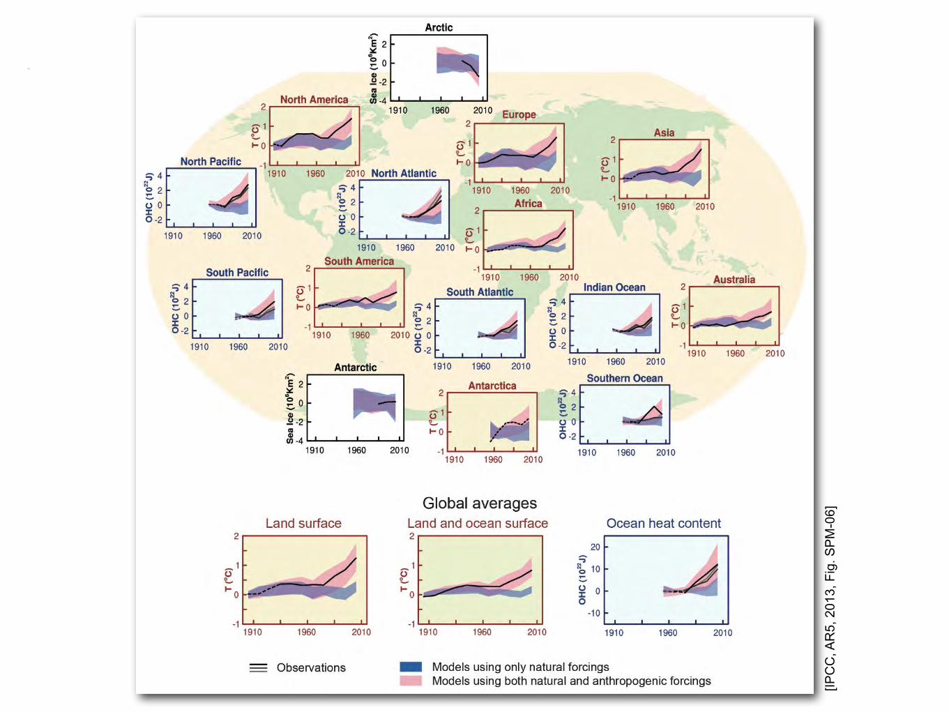
[IPC
C, A
R5,
201
3, F
ig. S
PM
-06]
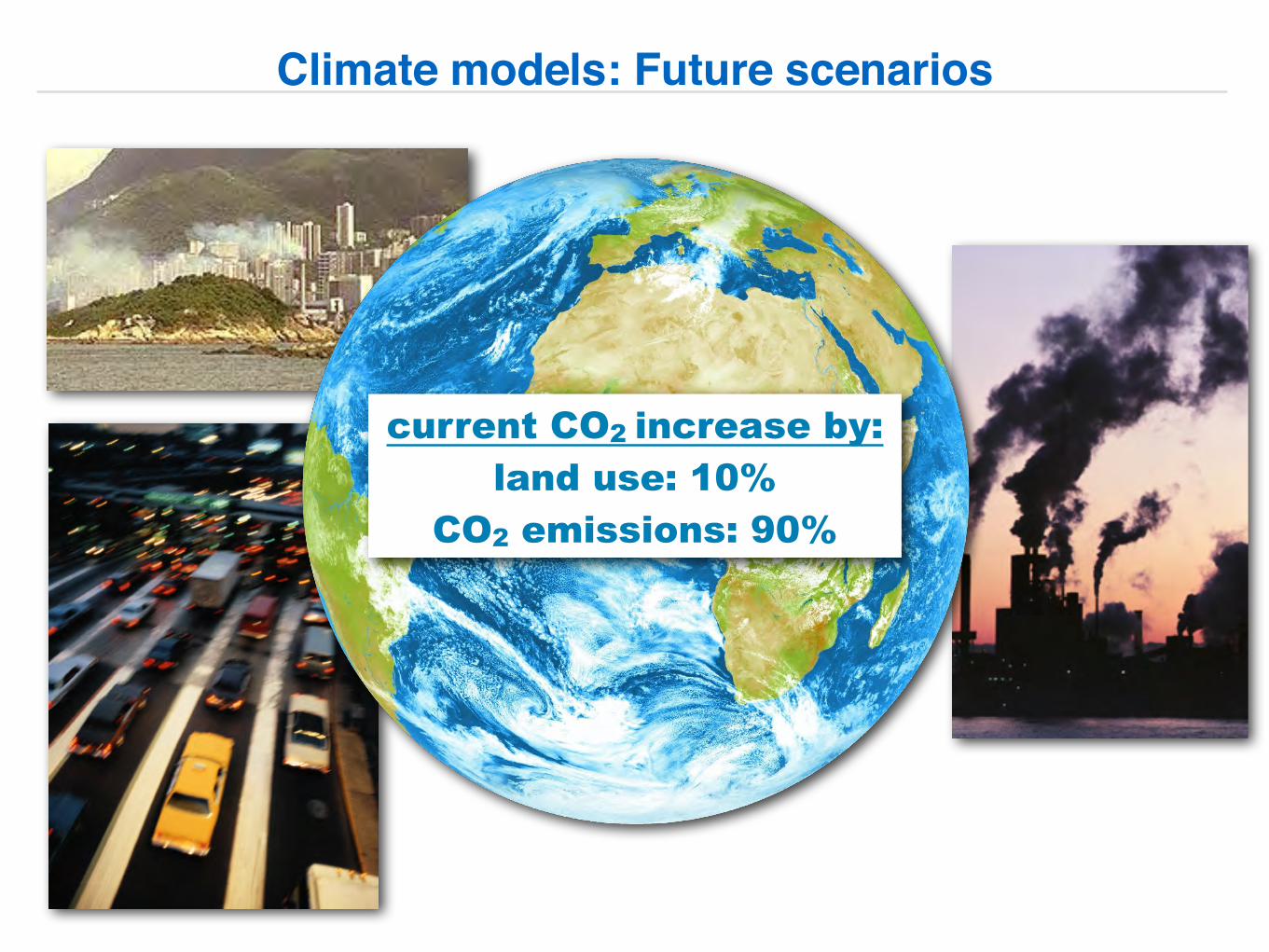
Climate models: Future scenarios
current CO2 increase by: land use: 10%
CO2 emissions: 90%
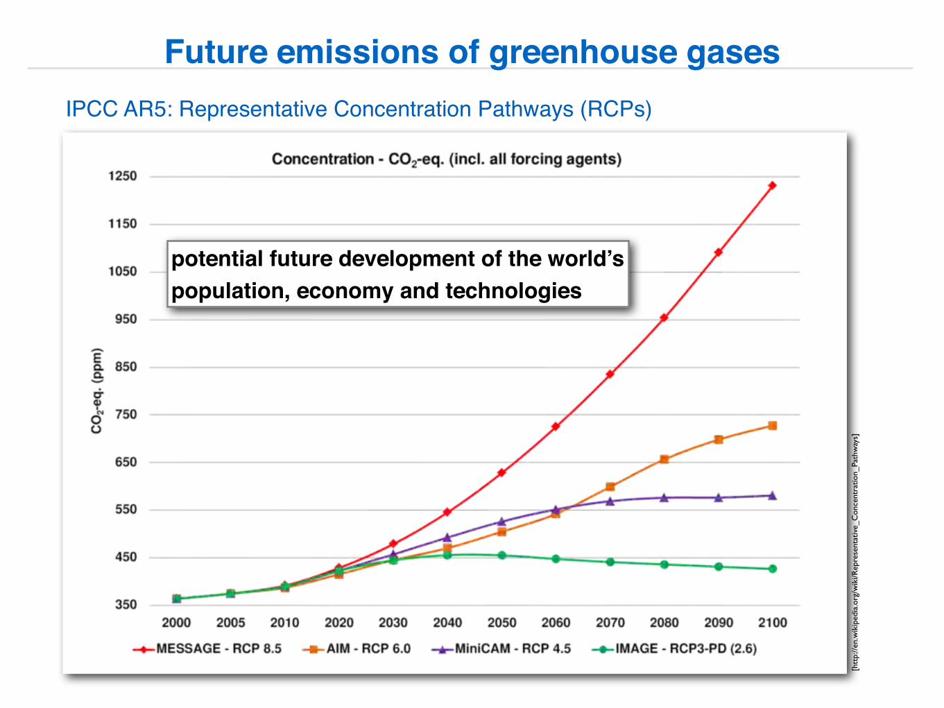
Future emissions of greenhouse gases
[htt
p://e
n.w
ikip
edia
.org
/wik
i/Rep
rese
ntat
ive_
Con
cent
ratio
n_Pa
thw
ays]
IPCC AR5: Representative Concentration Pathways (RCPs)
potential future development of the world’s population, economy and technologies
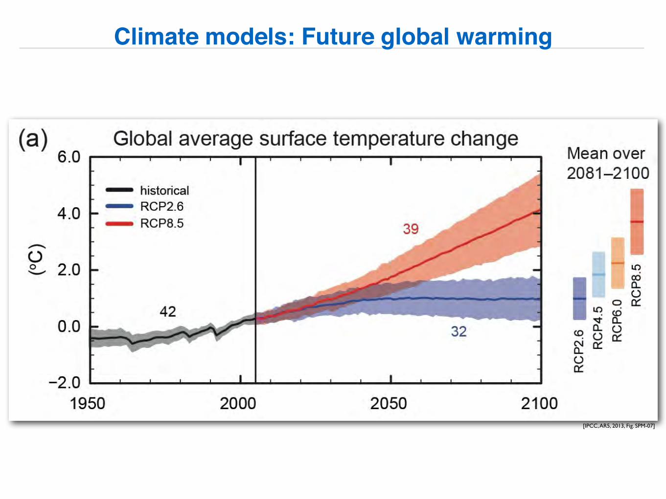
Climate models: Future global warming
[IPCC, AR5, 2013, Fig. SPM-07]
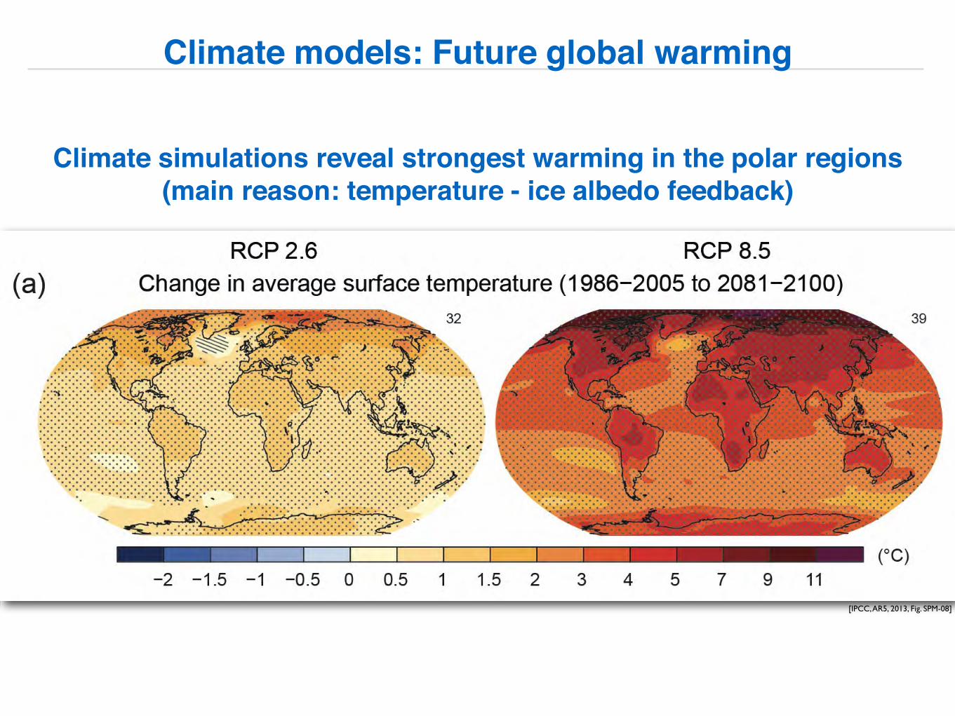
Climate simulations reveal strongest warming in the polar regions(main reason: temperature - ice albedo feedback)
Climate models: Future global warming
[IPCC, AR5, 2013, Fig. SPM-08]
8th lecture:Climate models
(Structure of climate models, components, climate scenarios: from past to the future)
Climate II (Winter 2020/2021)
End of lecture.
Slides available at:https://paleodyn.uni-bremen.de/study/climate2020_21.html