9-1

Chapter 9

Approximation Algorithms

9-2

Approximation algorithm Up to now, the best algorithm for

solving an NP-complete problem requires exponential time in the worst case. It is too time-consuming.

To reduce the time required for solving a problem, we can relax the problem, and obtain a feasible solution “close” to an optimal solution

9-3

The node cover problem Def: Given a graph G=(V, E), S is the node

cover if S V and for every edge (u, v) E, either u S or v S.

The node cover problem is NP-complete.

v2

v1

v5

v4

v3

The optimal solution:

{v2,v5}

9-4

An approximation algorithm

Input: A graph G=(V,E). Output: A node cover S of G.Step 1: S= and E’=E.Step 2: While E’ Pick an arbitrary edge (a,b) in E’. S=S{a,b}. E’=E’-{e| e is incident to a or b}

Time complexity: O(|E|)

9-5

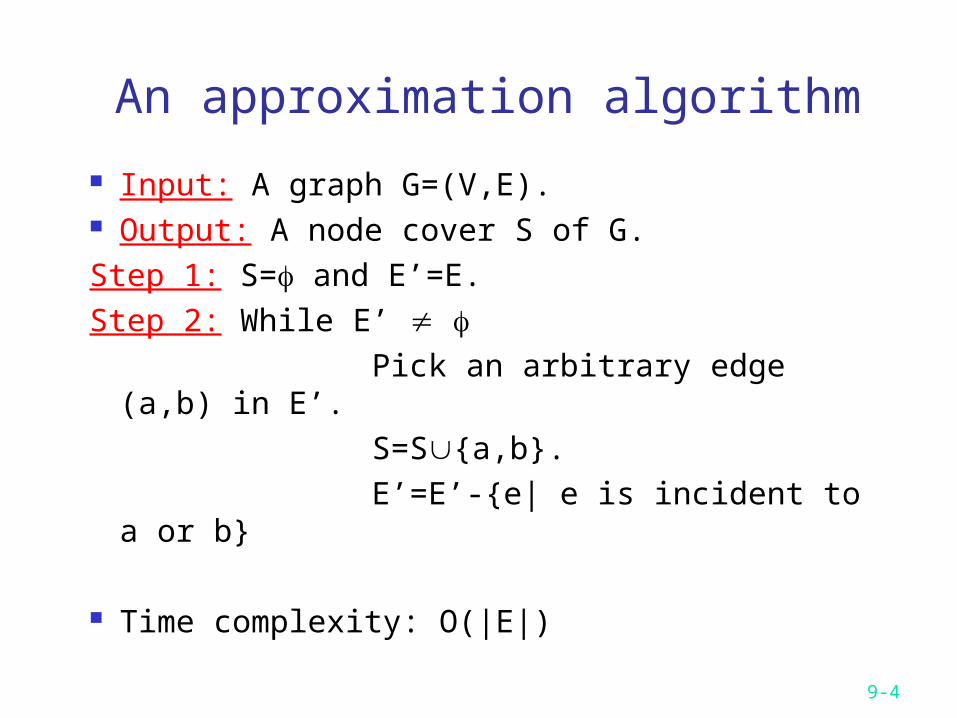
Example: First: pick (v2,v3)

then S={v2,v3 }

E’={(v1,v5), (v4,v5)}

second: pick (v1,v5)

then S={v1,v2,v3 ,v5}

E’=

v2

v1

v5

v4

v3

9-6

How good is the solution ? |S| is at most two times the minimum

size of a node cover of G. L: the number of edges we pick M*: the size of an optimal solution (1) L M*, because no two edges picked

in Step 2 share any same vertex. (2) |S| = 2L 2M*

9-7

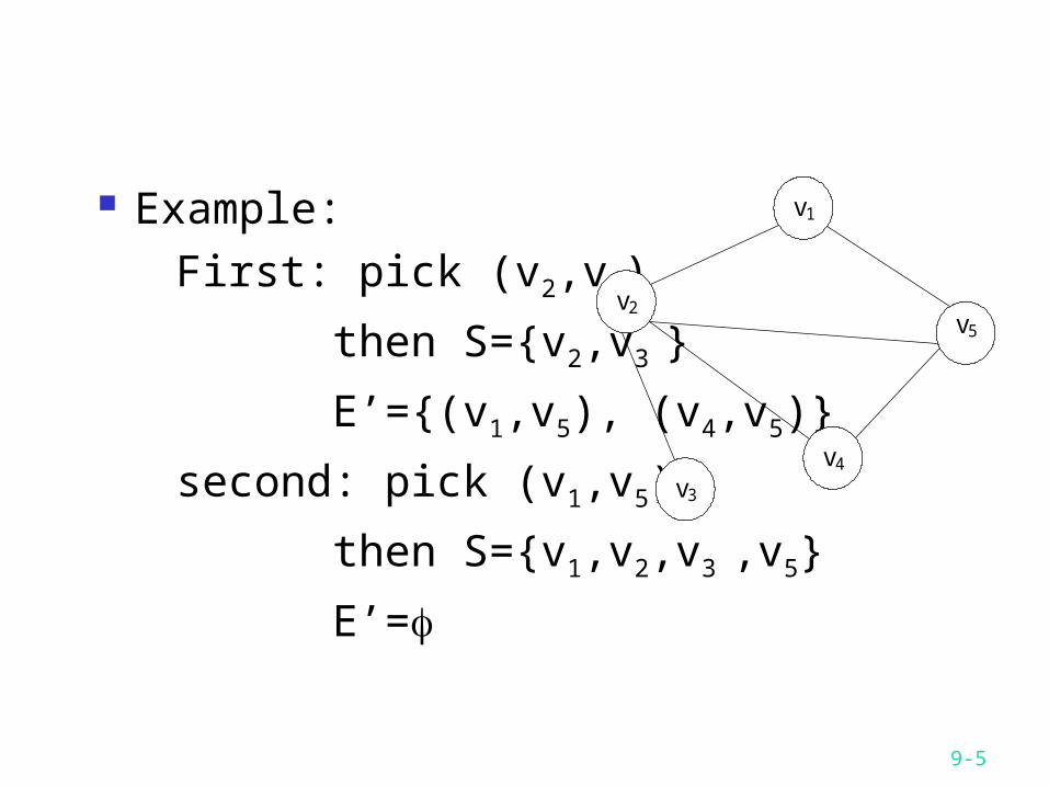
The Euclidean traveling salesperson problem (ETSP)

The ETSP is to find a shortest closed path through a set S of n points in the plane.

The ETSP is NP-hard.

9-8

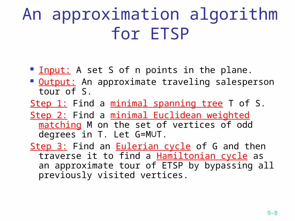
An approximation algorithm for ETSP

Input: A set S of n points in the plane. Output: An approximate traveling salesperson

tour of S.Step 1: Find a minimal spanning tree T of S.Step 2: Find a minimal Euclidean weighted

matching M on the set of vertices of odd degrees in T. Let G=M∪T.

Step 3: Find an Eulerian cycle of G and then traverse it to find a Hamiltonian cycle as an approximate tour of ETSP by bypassing all previously visited vertices.

9-9

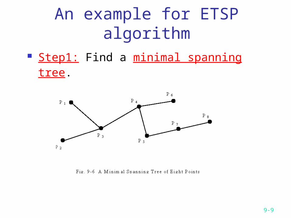
Step1: Find a minimal spanning tree.

An example for ETSP algorithm

9-10

Step2: Perform weighted matching. The number of points with odd degrees must be even because is even.

n

ii Ed

1

2

9-11

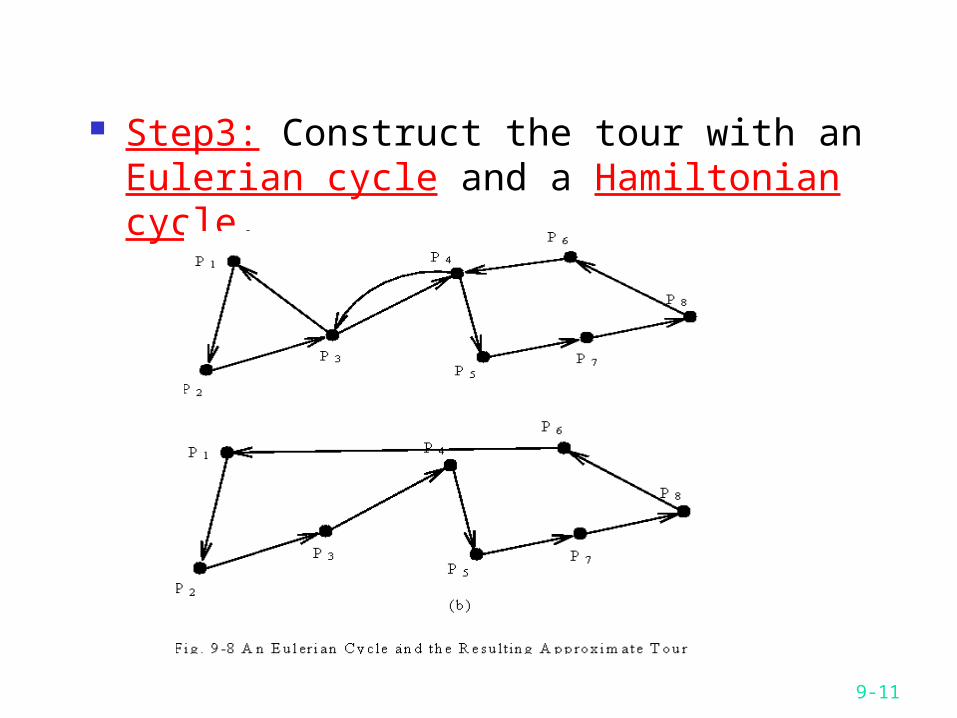
Step3: Construct the tour with an Eulerian cycle and a Hamiltonian cycle.

9-12

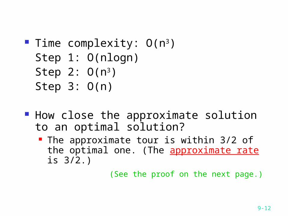
Time complexity: O(n3)Step 1: O(nlogn)Step 2: O(n3)Step 3: O(n)

How close the approximate solution to an optimal solution? The approximate tour is within 3/2 of the

optimal one. (The approximate rate is 3/2.) (See the proof on the next page.)

9-13

Proof of approximate rate optimal tour L: j1…i1j2…i2j3…i2m

{i1,i2,…,i2m}: the set of odd degree vertices in T.

2 matchings: M1={[i1,i2],[i3,i4],…,[i2m-1,i2m]}

M2={[i2,i3],[i4,i5],…,[i2m,i1]}

length(L) length(M1) + length(M2) (triangular inequality)

2 length(M ) length(M) 1/2 length(L ) G = T∪M length(T) + length(M) length(L) + 1/2 length(L) = 3/2 length(L)

9-14

The bottleneck traveling salesperson problem (BTSP)

Minimize the longest edge of a tour.

This is a mini-max problem. This problem is NP-hard. The input data for this problem

fulfill the following assumptions: The graph is a complete graph. All edges obey the triangular

inequality rule.

9-15

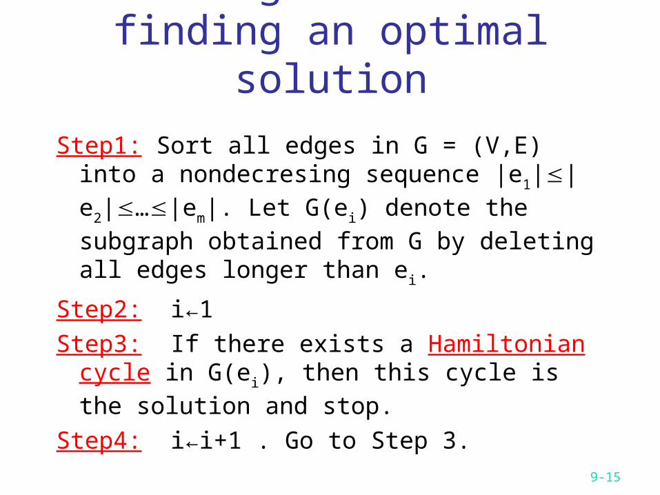
An algorithm for finding an optimal solution

Step1: Sort all edges in G = (V,E) into a nondecresing sequence |e1||e2|…|em|. Let G(ei) denote the subgraph obtained from G by deleting all edges longer than ei.

Step2: i←1Step3: If there exists a Hamiltonian cycle

in G(ei), then this cycle is the solution and stop.

Step4: i←i+1 . Go to Step 3.

9-16

An example for BTSP algorithm

e.g.

There is a Hamiltonian cycle, A-B-D-C-E-F-G-A, in G(BD).

The optimal solution is 13.

1

9-17

Theorem for Hamiltonian cycles

Def : The t-th power of G=(V,E), denoted as Gt=(V,Et), is a graph that an edge (u,v)Et if there is a path from u to v with at most t edges in G.

Theorem: If a graph G is bi-connected, then G2 has a Hamiltonian cycle.

9-18

An example for the theorem

A Hamiltonian cycle:

A-B-C-D-E-F-G-A

G2

9-19

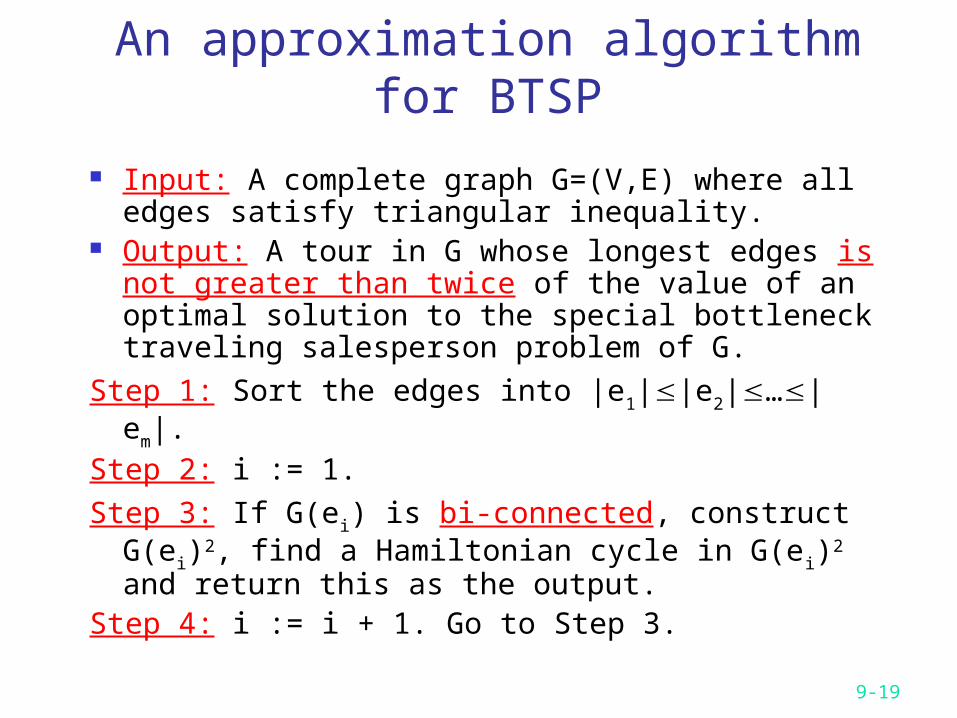
An approximation algorithm for BTSP

Input: A complete graph G=(V,E) where all edges satisfy triangular inequality.

Output: A tour in G whose longest edges is not greater than twice of the value of an optimal solution to the special bottleneck traveling salesperson problem of G.

Step 1: Sort the edges into |e1||e2|…|em|.Step 2: i := 1.

Step 3: If G(ei) is bi-connected, construct G(ei)2,

find a Hamiltonian cycle in G(ei)2 and return

this as the output.Step 4: i := i + 1. Go to Step 3.

9-20

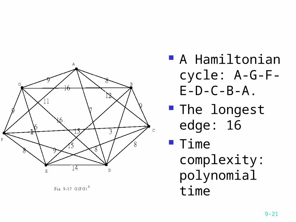
An example

Add some more edges. Then it becomes bi-connected.

9-21

A Hamiltonian cycle: A-G-F-E-D-C-B-A.

The longest edge: 16

Time complexity: polynomial time

1

9-22

How good is the solution ?

The approximate solution is bounded by two times an optimal solution.

Reasoning:A Hamiltonian cycle is bi-connected.

eop: the longest edge of an optimal solution

G(ei): the first bi-connected graph

|ei||eop|

The length of the longest edge in G(ei)22|ei|

(triangular inequality) 2|eop|

9-23

NP-completeness

Theorem: If there is a polynomial approximation algorithm which produces a bound less than two, then NP=P.(The Hamiltonian cycle decision problem reduces to this problem.)

Proof:For an arbitrary graph G=(V,E), we expand G to a complete graph Gc:

Cij = 1 if (i,j) E

Cij = 2 if otherwise

(The definition of Cij satisfies the triangular inequality.)

9-24

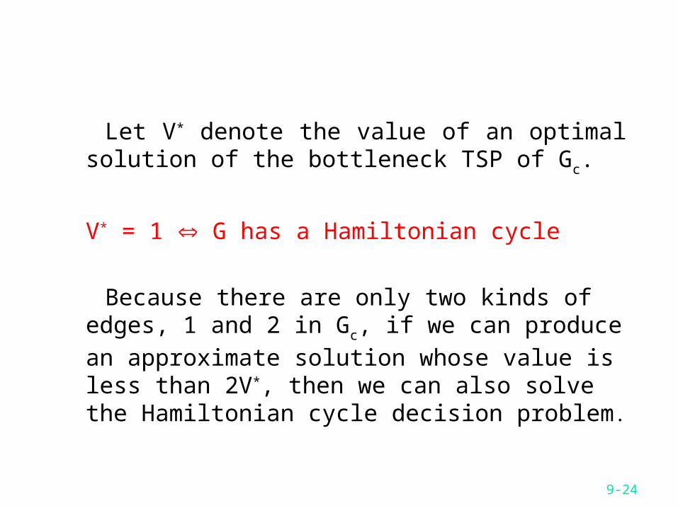
Let V* denote the value of an optimal solution of the bottleneck TSP of Gc.

V* = 1 G has a Hamiltonian cycle

Because there are only two kinds of edges, 1 and 2 in Gc, if we can produce an approximate solution whose value is less than 2V*, then we can also solve the Hamiltonian cycle decision problem.

9-25

The bin packing problem n items a1, a2, …, an, 0 ai 1, 1 i n,

to determine the minimum number of bins of unit capacity to accommodate all n items.

E.g. n = 5, {0.8, 0.5, 0.2, 0.3, 0.4}

The bin packing problem is NP-hard.

9-26

An approximation algorithm for the bin

packing problem

An approximation algorithm: (first-fit) place ai into the lowest-

indexed bin which can accommodate ai.

Theorem: The number of bins used in the first-fit algorithm is at most twice of the optimal solution.

9-27

Notations: S(ai): the size of item ai OPT: # of bins used in an optimal solution m: # of bins used in the first-fit algorithm C(Bi): the sum of the sizes of aj’s packed in bin Bi in the

first-fit algorithm

OPT

C(Bi) + C(Bi+1) 1

C(B1)+C(B2)+…+C(Bm) m/2

m < 2 = 2 2 OPT m < 2 OPT

n

iiaS

1

)(

m

iiBC

1

)(

n

iiaS

1

)(

Proof of the approximate rate

9-28

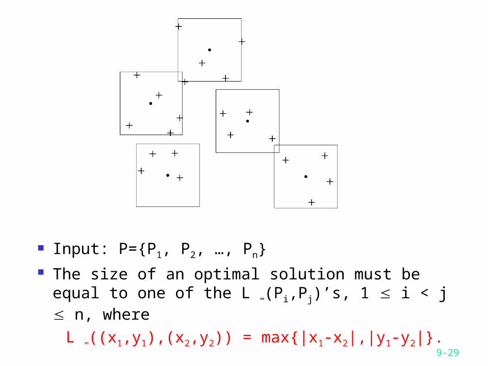
The rectilinear m-center problem

The sides of a rectilinear square are parallel or perpendicular to the x-axis of the Euclidean plane.

The problem is to find m rectilinear squares covering all of the n given points such that the maximum side length of these squares is minimized.

This problem is NP-complete. This problem for the solution with error

ratio < 2 is also NP-complete. (See the example on the next page.)

9-29

Input: P={P1, P2, …, Pn} The size of an optimal solution must be equal

to one of the L ∞(Pi,Pj)’s, 1 i < j n, where

L ∞((x1,y1),(x2,y2)) = max{|x1-x2|,|y1-y2|}.

9-30

An approximation algorithm

Input: A set P of n points, number of centers: m Output: SQ[1], …, SQ[m]: A feasible solution of the rectilinear m-center

problem with size less than or equal to twice of the size of an optimal solution.

Step 1: Compute rectilinear distances of all pairs of two points and sort them together with 0 into an ascending sequence D[0]=0, D[1], …, D[n(n-1)/2].

Step 2: LEFT := 1, RIGHT := n(n-1)/2 //* Binary searchStep 3: i := (LEFT + RIGHT)/2.Step 4: If Test(m, P, D[i]) is not “failure” then RIGHT := i-1 else LEFT := i+1Step 5: If RIGHT = LEFT then

return Test(m, P, D[RIGHT]) else go to Step 3.

9-31

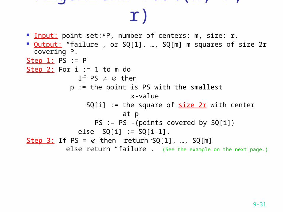
Algorithm Test(m, P, r) Input: point set: P, number of centers: m, size: r. Output: “failure”, or SQ[1], …, SQ[m] m squares of size 2r

covering P.Step 1: PS := PStep 2: For i := 1 to m do

If PS then p := the point is PS with the smallest

x-value SQ[i] := the square of size 2r with center

at p PS := PS -{points covered by SQ[i]}

else SQ[i] := SQ[i-1].Step 3: If PS = then return SQ[1], …, SQ[m] else return “failure”. (See the example on the next page.)

9-32

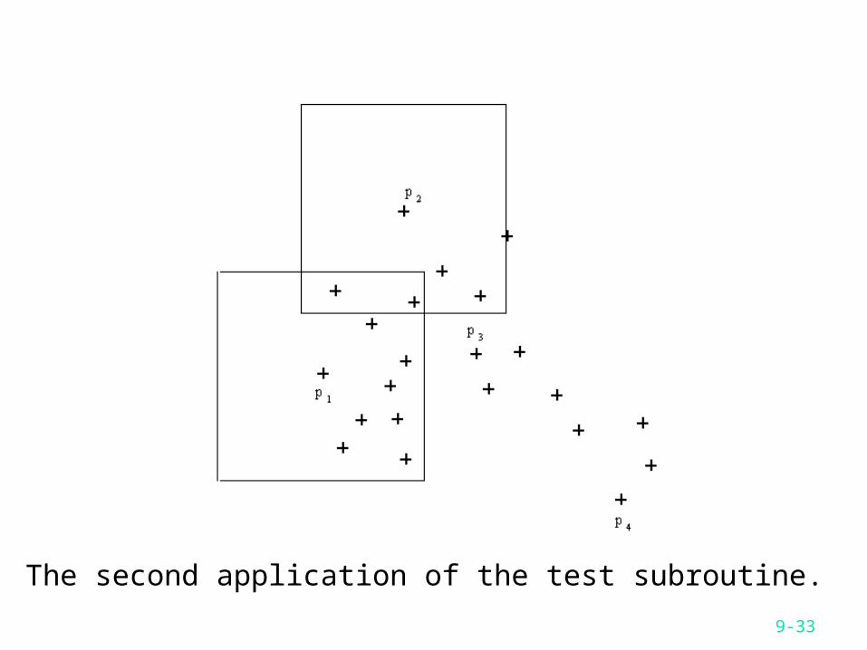
An example for the algorithm

The first application of the relaxed test subroutine.

9-33

The second application of the test subroutine.

9-34

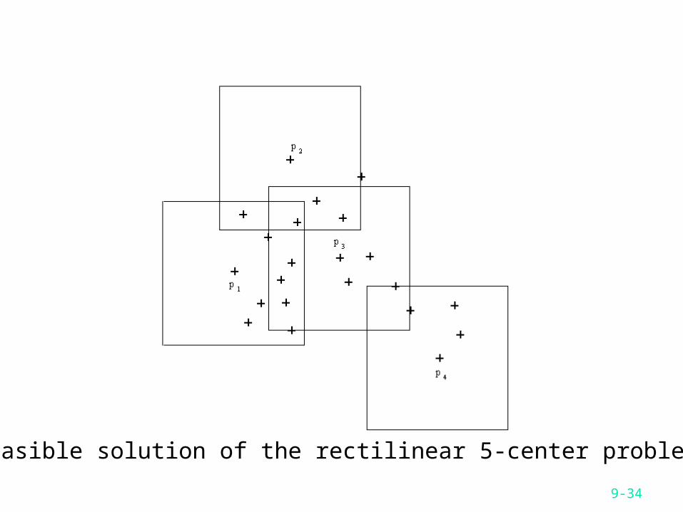
A feasible solution of the rectilinear 5-center problem.

9-35

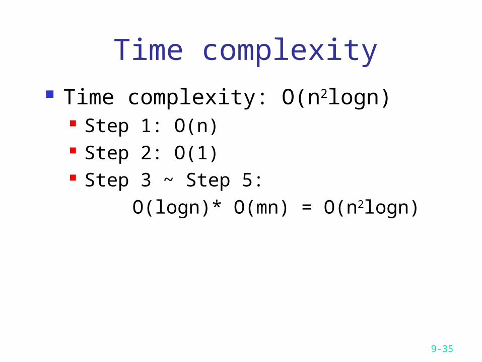
Time complexity Time complexity: O(n2logn)

Step 1: O(n) Step 2: O(1) Step 3 ~ Step 5: O(logn)* O(mn) = O(n2logn)

9-36

How good is the solution ? The approximation algorithm is of error

ratio 2. Reasoning: If r is feasible, then Test(m,

P, r) returns a feasible solution of size 2r.

The explanation of Si Si

’