90 IEEE TRANSACTIONS ON NEURAL NETWORKS, VOL. 19, NO. 1

90 IEEE TRANSACTIONS ON NEURAL NETWORKS, VOL. 19, NO. 1, JANUARY 2008

Generalized Hamilton–Jacobi–Bellman Formulation-Based Neural Network Control of Affine

Nonlinear Discrete-Time SystemsZheng Chen, Student Member, IEEE, and Sarangapani Jagannathan, Senior Member, IEEE

Abstract—In this paper, we consider the use of nonlinear net-works towards obtaining nearly optimal solutions to the controlof nonlinear discrete-time (DT) systems. The method is based onleast squares successive approximation solution of the generalizedHamilton–Jacobi–Bellman (GHJB) equation which appears inoptimization problems. Successive approximation using the GHJBhas not been applied for nonlinear DT systems. The proposed re-cursive method solves the GHJB equation in DT on a well-definedregion of attraction. The definition of GHJB, pre-Hamiltonianfunction, HJB equation, and method of updating the controlfunction for the affine nonlinear DT systems under small pertur-bation assumption are proposed. A neural network (NN) is usedto approximate the GHJB solution. It is shown that the result is aclosed-loop control based on an NN that has been tuned a prioriin offline mode. Numerical examples show that, for the linearDT system, the updated control laws will converge to the optimalcontrol, and for nonlinear DT systems, the updated control lawswill converge to the suboptimal control.

Index Terms—Generalized Hamilton–Jacobi–Bellman (BHJB)equation, neural network (NN), nonlinear discrete-time (DT)system.

I. INTRODUCTION

I N the literature, there are many methods of designing stablecontrol of nonlinear systems. However, stability is only a

bare minimum requirement in a system design. Ensuring op-timality guarantees the stability of the nonlinear system; how-ever, optimal control of nonlinear systems is a difficult and chal-lenging area. If the system is modeled by linear dynamics andthe cost function to be minimized is quadratic in the state andcontrol, then the optimal control is a linear feedback of thestates, where the gains are obtained by solving a standard Ric-cati equation [9]. On the other hand, if the system is modeled bythe nonlinear dynamics or the cost function is nonquadratic, theoptimal state feedback control will depend upon obtaining thesolution to the Hamilton–Jacobi–Bellman (HJB) [10] equation

Manuscript received May 28, 2006; revised December 21, 2006; acceptedApril 17, 2007. This work was supported in part by the National Science Foun-dation under Grants ECCS #0327877 and ECCS#0621924.

Z. Chen was with the Department of Electrical and Computer Engineering,University of Missouri—Rolla, Rolla, MO 65409-0910 USA. He is now with theDepartment of Electrical and Computer Engineering, Michigan State University,East Lansing, MI 48824 USA (e-mail: [email protected]).

S. Jagannathan is with the Department of Electrical and Computer Engi-neering, University of Missouri—Rolla, Rolla, MO 6540-0910 USA (e-mail:[email protected]).

Color versions of one or more of the figures in this paper are available onlineat http://ieeexplore.ieee.org.

Digital Object Identifier 10.1109/TNN.2007.900227

which is generally nonlinear. The HJB equation is difficult tosolve directly because it involves solving either nonlinear par-tial difference or differential equations.

To overcome the difficulty in solving the HJB equation, re-cursive methods are employed to obtain the solution of HJBequation indirectly. Kleinman [14] pointed out that the solu-tion of the Riccati equation can be obtained by successivelysolving a sequence of Lyapunov equations, which is linear inthe cost function of the system, and thus, it is easier to solvewhen compared to a Riccati equation, which is nonlinear inthe cost function. Saridis [11] extended this idea to the case ofnonlinear continuous-time systems where a recursive methodis used to obtain the optimal control of continuous system bysuccessively solving the generalized Hamilton–Jacobi–Bellman(GHJB) equation, and then, updating the control if an admissibleinitial control is given. There has been a great deal of effort to ad-dress this problem in the literature in continuous time. Approx-imate HJB solution has been confronted using many techniquesby Saridis [11], Beard [19]–[21], Bernstein [1], Bertsekas andTsitsiklis [2], Han and Balakrishnan [12], Lyshevski [15], Lewis[6], [7], and others.

Although the GHJB equation is linear and easier to solve thanHJB equation, no general solution for GHJB is demonstrated.Galerkin’s spectral approximation method is employed in [19]to find approximate but close solutions to the GHJB at each it-eration step. Beard [20] employed a series of polynomial func-tions as basic functions to solve the approximate GHJB equa-tion in continuous time but this method requires the compu-tation of a large number of integrals. Park [4] employed in-terpolating wavelets as the basic functions. On the other hand,Lewis and Abu-Khalaf [8], based on the work of Lyshevski [15],employed nonquadratic performance functional to solve con-strained control problems for general affine nonlinear contin-uous-time systems using neural networks (NNs). In addition, itwas also shown how to formulate the associated Hamilton–Ja-cobi–Isaac (HJI) equation using special nonquadratic supplyrates to obtain the nonlinear state feedback control. Huang[25], [26] reduced the gain optimization and nonlinearproblems to solving a single algebraic Riccati equation (ARE)along with a sequence of linear algebraic equations in discretetime (DT). Here, the value function is expanded by Taylor se-ries consisting of higher order terms into a series of polynomialfunctions and approximating them but this approach requiressignificant computations. Additionally, the ARE in DT is stillnonlinear which is difficult to solve.

Since NN can effectively extend adaptive control techniquesto nonlinearly parameterized systems, Miller [16] proposed

1045-9227/$25.00 © 2007 IEEE

CHEN AND JAGANNATHAN: GHJB FORMULATION-BASED NN CONTROL OF AFFINE NONLINEAR DT SYSTEMS 91

using NN to obtain optimal control laws via the HJB equa-tion. On the other hand, Parisini and Zoppoli [18] used NNto derive optimal control laws for DT stochastic nonlinearsystems. Similarly, Lin and Brynes [24] presented controlof DT nonlinear systems. Although many papers, i.e., [6],[7], [11], [19], and [20], have discussed the GHJB method forcontinuous-time systems, currently there is very minimal workavailable on the GHJB method for DT nonlinear systems. DTversion of the approximate GHJB-equation-based control is im-portant since all the controllers are typically implemented usingembedded digital hardware. Ferrari and Stengel [27] solvedDT HJB problem through adaptive critic designs (ACD). Thecost function and control is updated through heuristic dynamicprogramming (HDP), dual heuristic dynamic programming(DHP), global dual heuristic dynamic programming (GDHP),and action-dependent (AD) designs. Recent work on solvingHJB for continuous time has appeared in the edited book, where[27] was published.

In this paper, we will apply the idea of GHJB equation inDT and set up the practical method for obtaining the near-op-timal control of DT nonlinear systems by using Taylor seriesextension of the cost function. The higher terms (third orderand higher) in the Taylor series expansion of the cost or valuefunctional are ignored by using small signal perturbation as-sumption around the operating point while keeping a tradeoffbetween computation and accuracy. With an initial admissioncontrol, the cost function can be obtained by solving a so-calledGHJB equation in DT. Subsequently, the updated control is ob-tained by minimizing the pre-Hamiltonian function. It is alsodemonstrated that the updated control will converge to the op-timal control, which renders an approximate solution of the HJBequation in DT. The theory of GHJB in DT has also been appliedto the linear DT case which indicates that the optimal control isnothing but the solution of the standard Riccati equation.

We use successive approximation techniques by employingNN in the least squares sense to solve the GHJB in DT andusing the quadratic cost function. It is demonstrated that if theactivation functions of the NN are linearly independent, the NNweight matrix has a unique solution. It is also shown that the re-sult is a closed-loop control based on an NN that has been tuneda priori in offline mode. The theoretical results are verifiedthrough extensive rigorous simulation studies performed usinglinear and nonlinear DT systems and a two-link planar robotarm system. In the linear case, the updated control is shownto converge to the optimal control. In the nonlinear case, asexpected, the updated control will converge to the suboptimalcontrol.

It is also important to note that the proposed approach isdifferent than a conventional DT linear quadratic regulator(DTLQR). DTLQR will not render the same solution as that ofthe one presented in this paper as we have considered severalhigher order terms in the Taylor series expansion making itnonlinear and yet it is an approximated and sufficiently accuratemethodology. Additionally, similarities between dynamicalprogramming (DP) and GHJB theory and the differences be-tween GHJB theory in discrete and continuous time are alsohighlighted in this paper.

The remainder of this paper is organized as follows. Section IIintroduces the DT GHJB theory. The method of obtaining the

optimal control is discussed and verification for linear DT caseis given. The NN method to approximately solve the GHJBequation is described and the Galerkin’s spectral approxima-tion method is applied in Section III. The GHJB-based con-troller design is demonstrated on a linear and nonlinear DTsystem through simulation in Section IV. Additionally, we applythe GHJB method to obtaining the near-optimal control of atwo-link planar robot arm system. Finally, concluding remarksand future works are provided in Section V.

II. OPTIMAL CONTROL AND GHJB EQUATION FOR

NONLINEAR DT SYSTEMS

Consider an affine in the control nonlinear DT dynamicsystem of the form

(1)

where , , , and. Assume that is Lipschitz continuous

on a set in containing the origin, and that the system (1)is controllable in the sense that there exists a continuous controlon that asymptotically stabilizes the system. It is desired tofind a control function , which minimizes thegeneralized quadratic cost function

(2)

where is a positive–definite matrix, is a symmetric posi-tive–definite matrix, and is a final state punishmentfunction which is positive definite.

A. Control Objective

The objective is to select the feedback control law ofin order to minimize the cost-functional value.

Remark 1: It is important to note that the controlmust both stabilize the system on and make the cost-func-tional value finite so that the control is admissible [21].

Definition 2.1 (Admissible Controls): Let denote the setof admissible controls. A control functionis defined to be admissible with respect to the state penaltyfunction and control energy penalty function

on , denoted as , if the fol-lowing is true:

• is continuous on ;• ;• stabilizes system (1) on ;•

, .Remark 2: The admissible control guarantees that the control

converges but, in general, any converged control cannot guar-antee that it is admissible. For example, consider the nonlinearDT system

(3)


A feedback control is given as and the system solutionwill be

forfor

As , . This system with this feedback controlis considered stable. However, and thesum is infinite. We canconclude that this feedback control is stable but not admissible.Hence, we should restrict the systems that decay sufficientlyfast.

Given an admissible control and the state of the system atevery instant of time, the performance of this control is eval-uated through a cost function. If the solution of the dynamicsystem is known andgiven the cost function, the overall cost is the sum of the costvalue calculated at each time step . However, for complex non-linear DT systems, the closed-form solution is difficult todetermine and the solution can depend upon the initial condi-tions. Therefore, another suitable cost function, which is inde-pendent of the solution of the nonlinear dynamic system ,is needed. In general, it is very difficult to select the cost func-tion; however, Theorem 2.1 will prove that there exists a pos-itive–definite function , denoted in this paper for sim-plicity as , referred to as the value function, whose initialvalue is equal to the cost-functional value of givenan admissible control and the state of the system.

Theorem 2.1: Assume is an admissible controllaw arbitrarily selected for the nonlinear DT system. If there ex-ists a positive–definite, uniformly convex, and continuously dif-ferentiable value function on satisfying the following:

(4)

(5)

where and are the gradient vector and Hessianmatrix of , then is the value function of the systemdefined in (1) for all when the feedback control

is applied and

(6)

Proof: Assume that exists and is continu-ously differentiable. Then

(7)

where is the first differ-ence. Since is a continuously differentiable function,expanding the function using Taylor series about the op-erating point of renders

(8)

where is the gradient vector defined as

(9)

and is the Hessian matrix defined as

......

...

(10)

By assuming small perturbation about the operating point, the first three terms of Taylor series

expansion can be considered and we can ignore terms higherthan second order to receive

(11)

From (7) and (11), using system dynamics (1), we can get

(12)

where , , and . Forconvenience, we denote

(13)

Then, we rewrite (12) to get

(14)

Similarly, we rewrite (2) as

(15)We add (14) on both sides of (15) and rewrite (14) as


(16)

Because , from (4) and (5), we also have

(17)

(18)

Applying (17) and (18) into (16) renders

for (19)

More specifically, for , .Remark 3: An optimal control function for a non-

linear DT system is the one that minimizes the value function.

Remark 4: If is quadratic function of , since, then Theorem 2.1 can be applicable to

nonlinear DT systems without making the small perturbationassumption.

Definition 2.2 (GHJB Equation for Nonlinear DT System):

(20)

(21)

where .In this paper, the infinite-horizon optimal control problem for

the nonlinear DT system (1) is attempted. The cost function ofthe infinite-horizon problem for the DT system is defined as

(22)

The GHJB (20) with the boundary condition (21) can be used as(4) and (5) for the infinite-horizon problems, because, as

, and ;so if an admissible control is specified, for any infinite-horizonproblem, we can solve the GHJB equation to obtain the valuefunction which in turn can be used in the cost function

along with to calculate the cost of the admissiblecontrol.

We already know how to evaluate the performance of the cur-rent admissible control, but this is not our final goal. Our objec-tive is to improve the performance of the system over time byupdating the control so that a near-optimal controller can be ob-tained. Besides deriving an updated control law, it is requiredthat the updated control functions render admission control in-puts to the nonlinear system while ensuring that the performance

is enhanced over time. The updated control function is obtainedby minimizing a pre-Hamiltonian function. In fact, Theorem 2.2demonstrates that if the control function is updated by mini-mizing the pre-Hamiltonian function defined in (23), then thesystem performance can be enhanced over time while guaran-teeing that the updated control function is admissible for theoriginal nonlinear system (1). Next, the pre-Hamiltonian func-tion for the DT system is introduced.

Definition 2.3 (Pre-Hamiltonian Function for the NonlinearDT System): A suitable pre-Hamiltonian function for the non-linear system (1) is defined as

(23)

where . It is important to note that the pre-Hamiltonianis a nonlinear function of the state and cost value functionthe control functions. If a control function and cost valuefunction satisfy , an updated control functionGHJB can be obtained by differentiatingthe pre-Hamiltonian function (23) associated with the valuefunction . In other words, the updated control function canbe obtained by solving

(24)

so that

(25)

In Theorem 2.1, since the positive–definite function is uni-formly convex on , is a positive–definite functionon and the matrix is positive definite; so it can be concludedthat is a positive–definite matrix on

. We can rewrite (25) as

(26)

Theorem 2.2 demonstrates that the updated control function isnot only an admissible control but also improved control for thenonlinear DT system described by (1).

Theorem 2.2 (Improved Control): If andand the positive–definite and convex function

satisfies GHJB with the boundary condition, then the updated control function derived in (26)

by using the pre-Hamiltonian results in an admissible controlfor the system (1) on . Moreover, if is the unique pos-itive–definite function satisfying GHJB ,then

(27)


Proof of Admissibility: First, we should investigate the sta-bility of the system with the control . We take the differ-ence of along the system trajectories toobtain

(28)

Rewriting the GHJB equation GHJB for, we have

(29)

Substituting (29) into (28), (28) can be rewritten as

(30)

Substituting (26) into (30), the difference can be obtained as

(31)

Since and and are positive–definite ma-trixes, we get

(32)This implies that the difference of along the system

trajectories is negative for . Thus,is a Lyapunov function for on and the system

with feedback control is locally asymptotically stable.Second, we need to prove that the cost function of the system

with the updated control is finite. Since is an admis-sible control, from Definition 2.1 and (4), we have

for (33)

The cost function for can be written as

(34)

where is the trajectory of system with admission control. From (31) and (34), we have

(35)

Since and , we get. Rewriting (35), we have

(36)

From (33) and (36), and considering that is apositive–definite matrix function, we obtain

(37)Third, since is continuously differentiable and

is a Lipschitz continuous function on the set in , thenew control law is continuous. Since is a posi-tive–definite function, it attains a minimum at the origin, andthus, and must vanish at the origin. Thisimplies that .

Finally, following the Definition 1.1, one can conclude thatthe updated control function is admissible on .

Proof of the Improved Control: To show the secondpart of the Theorem 2.2, we need to prove that

which means the cost function will be reducedby updating the feedback control. Because is an admis-sible control, there exists a positive–definite functionsuch that on . Accordingto the Theorem 2.1, we can get

(38)

From (36) and (38), we know that

(39)

Theorem 2.2 suggests that after solving the GHJB equation andupdating the control function by using (26), the system perfor-


mance can be improved. If the control function is iterated suc-cessively, the updated control will converge close to the solutionof HJB, which then renders the optimal control function. TheGHJB becomes the Hamilton–Jacobi–Bellman (HJB) equationon substitution of the optimal control function . The HJBequation can now be defined in DT as follows.

Definition 2.4 (HJB Equation for the Nonlinear DT): TheHJB equation in DT in this framework can be expressed as

(40)

(41)

where the optimal control function for the DT system is givenby

(42)

Note is the optimal solution to the HJB (40). It is impor-tant to note that the GHJB is linear in the value function deriva-tive while the HJB equation is nonlinear in the value functionderivative. Solving the GHJB equation requires solving linearpartial difference equations, while the HJB equation solution in-volves nonlinear partial difference equations, which may be dif-ficult to solve. This is the reason for introducing the successiveapproximation technique using GHJB. In the successive approx-imation method, one solves (20) for given a stabilizingcontrol , and then, finds an improved control based onusing (26). In the following, Corollary 2.1 indicates that if theinitial control function is admissible, then repetitive applicationof (20) and (26) is a contraction map, and the sequence of solu-tions converges to the optimal HJB solution .

Corollary 2.1 (Convergence of Successive Approximations):Given an initial admissible control by iterativelysolving GHJB (20) and updating the control function using (26),the sequence of solutions will converge to the optimalHJB solution .

Proof: From the proof of Theorem 2.2, it is clear that afteriteratively solving the GHJB equation and updating the control,the sequence of solutions is a decreasing sequence with alower bound. Since is a positive–definite function,

, and , the sequence of solutions willconverge to a positive–definite function ,when . Due to the uniqueness of solutions of the HJBequation [11], now it is necessary to show that . When

, from (39), we can only obtain. Using (26) and taking , we obtain

(43)

The GHJB equation for can now be expressed as

(44)

(45)

From (43)–(45), we can conclude that these equations arenothing but the well-known HJB equation, which is presented inDefinition 2.4. This implies that converges to andconverges to .

Note that (40)–(42) are the HJB equations under the smallperturbation assumption. The more general and ideal HJB equa-tions are, then

(46)

(47)

where is the solution of

(48)

The ideal GHJB equations are given by

(49)

(50)

Although for the given admissible control , the idealGHJB (46) can be solved using an NN to get . However,without the small perturbation assumption, the updated controllaw cannot be easily solved from

(51)Additionally, it is quite difficult to show as an admis-sible and improved control.

Next, we show the consistency between proposed GHJB andDP using small perturbation assumption.

Remark 5: Consistency Between GHJB and DP: From theDP principle [2], the optimal controller can be given as

(52)

However, the optimal controller for a general nonlinear DTsystem is difficult to design and only for the special case of linearsystems, when can be solved in terms of and not interms of . But consider the derivative of functionexpressed as

(53)


Since the small perturbation assumption is considered, the high-order terms in Taylor expansion of can be ignored to get

(54)

Considering system (1), (54) can be rewritten as

(55)

Using (55), (52) can be written as

(56)By solving in (56), we can obtain

(57)Equation (57) shows that can be solved only in terms of

under the assumption that higher than second-order termsin the Taylor series expansion can be ignored. Equation (52)is consistent with (42). It is important to note that nonlinearapproximation theory will be utilized later to approximate thevalue function which provides a tradeoff between computationand accuracy. In summary, the value function in the proposedmethod is approximated and iterated until convergence. Then,the policy iteration is performed using the optimal value func-tion. The value and policy iterations are quite similar to the caseof approximate DP [16].

In order to verify HJB for a linear DT system, the proposedapproach is utilized next.

Remark 6: The ARE associated with the optimal control oflinear DT system can be derived from the DT HJB equation.Consider the following linear DT system and cost function de-fined in (22) as:

(58)

where and is a symmetric positive–definitematrix. The gradient vector and Hessian matrix of can bederived as and . The HJB (40)and (42) can be rewritten as

(59)

(60)

After simplifying (59) and (60), we obtain

(61)

(62)

Equation (61) is nothing but ARE [9] for linear DT system and(62) is the optimal control of linear DT system. Next, we showthe difference between GHJB in continuous and DT.

Remark 7: Difference Between GHJB in Continuous- andDiscrete-Time Systems With Small Perturbation: When the first-order term in Taylor extension of cost function is consid-ered alone, (8) can be rewritten as

(63)

By following the same steps in Theorems 2.1 and 2.2, we canobtain GHJB equation for this case

(64)

(65)

and the updated control law

(66)

These equations are nothing but the GHJB equations in con-tinuous time [21]. If the second-order terms from the Taylor se-ries expansion of the cost function are considered, the GHJBequations in DT derived in this paper show improvements in ap-proximating the cost function provided the perturbation is suffi-ciently small. In many cases, the cost function is quadraticfunction in . Then, cost function and also the optimalcontrol can be exactly calculated by the proposed GHJBmethod. Therefore, the proposed GHJB in DT appears to bemore accurate than directly applying the continuous-time GHJBmethod to a nonlinear DT system.

By considering the higher order terms, approximation accu-racy can be improved but a tradeoff exists between accuracy andcomputational complexity for practical realization of optimalcontrol [11]. Therefore, for practical design considerations, costor value function should be approximated using the aforemen-tioned approach.

III. NN LEAST SQUARES APPROACH

In Section II, we described that by recursively solving theGHJB equation and by updating the control function, we couldimprove the closed-loop performance of control laws that areknown to be admissible. Furthermore, we can get arbitrarilyclose to the optimal control by iterating the GHJB solutionenough number of times. Although the GHJB equation is intheory easier to solve than the HJB equation, there is no generalclosed-form solution available to this equation. In [19], Beardused Galerkin’s spectral method to get approximate solutionto GHJB in continuous time at each iterating step and theconvergence is shown in the overall run. This technique doesnot set the GHJB equation to zero at each iterating step, but toa residual error instead. The Galerkin spectral method requiresthe computation of a large number of integrals in order tominimize this residual error.

The purpose of this section is to show how we approximatethe solution of the GHJB equation in DT using NNs such thatthe controls which result from the solution are in feedback form.It is well known that NNs can be used to approximate smooth


functions on prescribed compact set [6]. We approximatewith an NN

(67)

where the activation function vector is con-tinuous, , the NN weights are , and isthe number of hidden layer neurons. The vectors

andare the vector of activation function and NN weight matrix,respectively. The NN weights will be tuned to minimize theresidual error in a least squares sense over a set of points withinthe stability region of the initial stabilizing control. Leastsquares solution [5] attains the lowest possible residual errorwith respect to the NN weights.

For the GHJB , is replaced by having aresidual error as

GHJB (68)

To find the least squares solution, the method of weighted resid-uals is used [5]. The weights are determined by projectingthe residual error onto and setting the resultto zero , i.e.,

(69)

When expanded, (69) becomes

(70)

where

In order to proceed, the following technical results are needed.Lemma 3.1: If the set is linearly independent and

, then the set

(71)

is also linearly independent.Proof: Calculating the along the system trajecto-

ries for by using the similar formulation of(7) and (11), we have

(72)

Since is an admissible control, the system isstable and . With the condition on the active function

, we have . Rewriting (72) withthe previous results, we have

(73)

Extending (73) into the vector formulation gives

(74)

Now, suppose that the Lemma 3.1 is not true. Then, there existsa nonzero such that

for

(75)From (74) and (75), we have

for (76)

which contradicts the linear independence of ; so theset (71) must be linearly independent. Equation (76) can berewritten, after defining

as

(77)

Because of Lemma 3.1, the term is full rank, and thus,is invertible. Therefore, a unique solution for exists. From(77), we need to calculate the inner product of . InHilbert space, we define the inner product as

(78)

Executing the integration in (78) is computationally expensive.However, the integration can be approximated to a suitable de-gree using the Riemann definition of integration so that the innerproduct can be obtained. This in turn results in a nearly optimal,computationally tractable solution algorithm.

Lemma 3.2 (Riemann Approximation of Integrals): An inte-gral can be approximated as

(79)

where and is bounded on [3].Introducing a mesh on , with mesh size equal to , which is

taken very small, we can rewrite some terms in (77) as (80) and


(81), shown at the bottom of the page, where in representsthe number of points of the mesh. This number increases as themesh size is reduced. Using Lemma 3.2, we can rewrite (70) as

(82)

This implies that we can calculate

(83)

An interesting observation is that (83) is the standard leastsquares method of estimation for a mesh on . Note that themesh size should be such that the number of points isgreater or equal to the order of the approximation and theactivation functions should be linearly independent. Theseconditions guarantee a full rank for .

The optimal control of nonlinear DT system can be obtainedoffline by going through the following six steps.

1) Define an NN as to approximatesmooth function of .

2) Select an admissible feedback control law .3) Find associated with to satisfy GHJB by applying

least square method (LSM) to obtain the NN weights ;4) Update the control as

(84)

5) Find associated with to satisfy GHJB by usingLSM to obtain .

6) If , where is a small positive constant,then and stop. Otherwise, go back to step 4) byincreasing the index by one.

After we get , the optimal state feedback control, which canbe implemented online, can be described as

(85)

IV. NUMERICAL EXAMPLES

The power of the technique is demonstrated for the case ofHJB by using three examples. First, we take on a linear DTsystem to compare the performance of the proposed approachto that of the standard solution obtained by solving Riccatiequation. This comparison will present that the proposedapproach works for a linear system and renders an optimalsolution. Second, we will use a general nonlinear practicalsystem and a real-world two-link planar revolute–revolute (RR)

robot arm system to demonstrate that the proposed approachrenders a suboptimal solution for nonlinear DT systems.

In all of the examples that we present in this section, the basisfunctions required will be obtained from even polynomials sothat the NN can approximate the positive–definite function orvalue function. If the dimension of the system is and the orderof approximation is , then we use all of the terms in expansionof the polynomial [21]

(86)

The resulting basis functions for a 2-D system is

(87)

1) Example 1 (Linear DT System): Consider the linear DTsystem (52), where

(88)

Define the cost function

(89)

Define the NN with the activation functions containing polyno-mial functions up to the sixth order of approximation by using

and . From (86), the NN can be constructed as

(90)Select the initial control law , which is admis-sible. Update the control with

(91)

where and satisfy the GHJB equation

(92)

In the simulation, the mesh size is selected as 0.01 and theasymptotic stability region is chosen for the states as

(80)

... (81)


Fig. 1. Cost function at each updating step.

Fig. 2. Norm of NN weights at each updating step.

and . The small positive approx-imation error constant is selected as . The initialstates are selected as . The simulationstep is selected as . After updating five times, theoptimal value function and the optimal control are ob-tained. Fig. 1 shows the cost-functional value and Fig. 2 showsthe norm of NN weights at each updating step. From these plots,it is clear that the cost-functional value continues to decreaseuntil it reaches a minimum and, afterwards, it remains constant.

After we obtain the optimal control based on the GHJBmethod, we implement the initial admissible control and theoptimal control on the system, respectively. Fig. 3 shows the

trajectory with an initial admissible control, whereasFig. 4 illustrates the trajectory with the GHJB-basedoptimal control. From these figures, we can conclude that theupdated control is not only an admissible control but it also

Fig. 3. State trajectory (x ; x ) with the initial control.

Fig. 4. State trajectory (x ; x ) with the GHJB-based optimal control.

TABLE ICOST VALUE WITH ADMISSIBLE CONTROLS

converges to the optimal control.Table I presents this withdifferent initial admissible controls we arbitrarily selected; thefinal NN weights, the optimal cost-functional values, and theupdated control function will converge to the unique optimalcontrol. This method is independent on the selection of theinitial admissible control for the linear DT systems.


Fig. 5. State trajectory (x ; x ) with Riccati-based optimal control.

Fig. 6. Difference between the two optimal controls.

In order to evaluate whether the proposed method convergesto the optimal control obtained from classical optimal controlmethods, we use the Riccati equation in DT to solve the LQRoptimal control problem for this system [9]. Riccati equation inDT is given by [9]

(93)

(94)

(95)

Fig. 5 displays that the optimal trajectory generatedby solving Riccati equation whereas Fig. 6 depicts the errorbetween the control inputs obtained from the proposed and the

TABLE IICOMPARISON OF CONTROL METHODS

Fig. 7. Cost-functional value of at each updating step.

Riccati methods. Table II shows the optimal cost-functionalvalue obtained from the two methods. Comparing Fig. 5 withFig. 3, and from Fig. 6 and Table II, we can observe that thetrajectories and the optimal control inputs are the same. Wecan conclude that for linear DT system, the updated controlassociated with GHJB equation will converge to the optimalcontrol.

2) Example 2 (Nonlinear DT System): Consider the non-linear DT system given by

(96)

where

(97)

We select the initial control law as and theNN is also selected from (90). The simulation parameters andcost function are defined the same as in the Example 1. Fig. 7shows the cost-functional value at each updating time and Fig. 8shows the norm of NN weights. After updating 11 times, weget the optimal control offline, and then, the optimal con-trol is implemented with several initial conditions. Fig. 9 showsthe state trajectory with initial admissible control. Bycontrast, Fig. 10 shows the state trajectory by solvingthe GHJB-based control with successive approximation. Dif-ferent values of initial admissible controls are used to obtain thenear-optimal control result. Table III shows, with different ini-tial admissible controls, that the final norm of NN weights and


Fig. 8. Norm of NN weights at each updating step.

Fig. 9. State trajectory with initial admissible control.

the optimal cost-functional value are almost the same demon-strating the validity of the proposed GHJB-based solution.

3) Example 3 (Two-Link Planar RR Robot Arm System): Atwo-link planar RR robot arm used extensively for simulationin the literature is shown in Fig. 11. This arm is simple enoughto simulate yet has all the nonlinear effects common to generalrobot manipulators. The DT dynamics of the two-link robotarm system is obtained by discretizing the continuous-timedynamics. In simulation, we apply the GHJB-based near-op-timal control method to solve the nonlinear quadratic regulatorproblem. In other words, we seek a suboptimal control tomove the arm to the desired position while minimizing thecost-functional value.

Fig. 10. State trajectory with GHJB-based optimal control.

TABLE IIIGHJB-BASED NEAR-OPTIMAL CONTROL WITH INITIAL ADMISSIBLE CONTROL

Fig. 11. Two-link planar robot arm.

The continuous-time dynamics model of two-link planar RRrobot is given [6] as

(98)

where , , , and. We define the state and control variables as


and . For simula-tion purposes, the parameters are selected as 1 kg,

1 m, and 10 m/s ; then, , , ,and . Rewriting the continuous-time dynamics as stateequation, we get

(99)

where (100) and (101), shown at the bottom of the page,hold. The control objective is moving the arm from an ini-tial state to the final state

with the cost function defined as

(102)

First, we will convert the continuous-time dynamics system andcost function into DT. Let us consider a DT system with a sam-pling period and denote a time function at as

, where is a sampling number. If the sampling periodis sufficiently small compared to the time constant of the system,the response evaluated by DT methods will be reasonably accu-rate [9]. Therefore, we use the following approximation for thederivative of :

(103)

Using this relation with the sampling interval of 1 ms,the continuous-time dynamics system can be converted to anequivalent DT nonlinear system as

(104)

where (105) and (106), shown at the bottom of the page, hold,with cost-functional value in DT chosen as

(107)

where and . The problem solu-tion is almost the same as the linear system example except thatwe move the original point of axis toand use the new axis as . The NN toapproximate the GHJB equation is selected as polynomial func-tions for up to the fourth order of approximation, which meansthat and . From (86), the NN can be constructedas

(108)

Associated gradient vector and Hessian matrix are derived as

(100)

(101)

(105)

(106)


Fig. 12. Cost function at each updating step.

(109)

We select the initial admissible control law as

(110)

Control function updating rule is taken as

(111)

The and satisfy the GHJB equation

In the simulation, the mesh size is selected as 0.2, the asymp-totic stability region is chosen as , ,

, and . The small positive constantis selected as . The simulation steps are selected as

. We use the GHJB method to obtain the near-optimalcontrol. After updated five times, the control has converged tothe suboptimal control . Fig. 12 shows the cost-functionalvalue over updating step. On the other hand, Fig. 13 shows thenorm of the NN weights at each updating step.

After we get the optimal control, we implement the initial ad-missible and suboptimal controls on the two-link planar robotarm system, respectively. Fig. 14 displays the state trajectory

with the initial admissible control and GHJB-based

Fig. 13. Norm of the weights at each updating step.

Fig. 14. State trajectory of (x ; x ).

suboptimal control. Similarly, Fig. 15 illustrates the state tra-jectory with initial admissible and GHJB-based subop-timal control. From these trajectory figures, we know that therobot arm has moved from the starting point to the final goal.On the other hand, Fig. 16 depicts the initial admissible control

and GHJB-based suboptimal control and Fig. 17 depictsthe initial admissible control and GHJB-based suboptimalcontrol . Table IV shows that with different initial admissiblecontrols, the converged norm of the NN weights and the sub-optimal cost-functional values are almost close to each other. Itis important to note that with different admissible control func-tion values, the successive approximation-based updated con-trols will converge to a unique improved control and the im-


Fig. 15. State trajectory of (x ; x ).

Fig. 16. Initial control � and suboptimal control � .

proved cost function values are almost the same. Since a smallfunction approximation error value is used in solving the GHJBequation, the approximation-based GHJB solution renders thesuboptimal control, which is quite close to the optimal controlsolution.

From Fig. 14, the trajectory with suboptimal control is a littlelonger than the trajectory with initial admissible control eventhough the cost-functional value with GHJB-based suboptimalcontrol is significantly lower. This is due to the tradeoff ob-served between the trajectory selection and energy of the con-trol input. The selection of the weighting and matrices will

Fig. 17. Initial control � and suboptimal control � .

Fig. 18. State trajectory (x ; x ) with suboptimal control.

dictate the selection. If we are more interested in perfect trajec-tory, we can select higher or reduce . If we are moreinterested in saving control energy, we can select lower orincrease . For example, if we select and

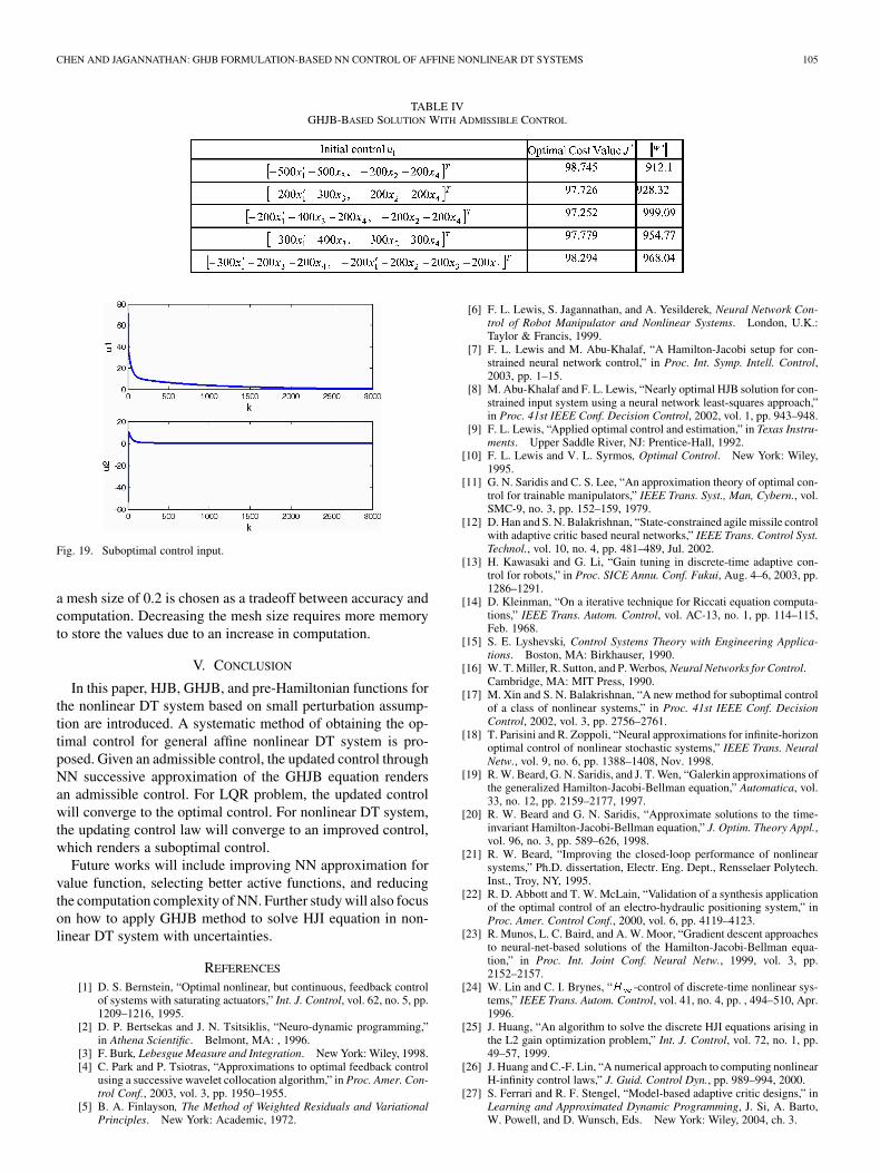
, Figs. 18 and 19 show that the results obtainedare different from those of Figs. 14, 16, and 17. It is importantto note that the trajectory in Fig. 18 is close to a straight line butat the expense of the control input.

In Table IV, optimal cost values with different initial con-trol are not exactly the same as those of the previous two ex-amples, but are still reasonable due to the selection of the meshsize of 0.2. By decreasing the mesh size, one can increase theaccuracy of convergence in the cost function. In the previoussecond-order system examples, the mesh size is selected as 0.01,which is quite small. However, in the fourth-order robot system,


TABLE IVGHJB-BASED SOLUTION WITH ADMISSIBLE CONTROL

Fig. 19. Suboptimal control input.

a mesh size of 0.2 is chosen as a tradeoff between accuracy andcomputation. Decreasing the mesh size requires more memoryto store the values due to an increase in computation.

V. CONCLUSION

In this paper, HJB, GHJB, and pre-Hamiltonian functions forthe nonlinear DT system based on small perturbation assump-tion are introduced. A systematic method of obtaining the op-timal control for general affine nonlinear DT system is pro-posed. Given an admissible control, the updated control throughNN successive approximation of the GHJB equation rendersan admissible control. For LQR problem, the updated controlwill converge to the optimal control. For nonlinear DT system,the updating control law will converge to an improved control,which renders a suboptimal control.

Future works will include improving NN approximation forvalue function, selecting better active functions, and reducingthe computation complexity of NN. Further study will also focuson how to apply GHJB method to solve HJI equation in non-linear DT system with uncertainties.

REFERENCES

[1] D. S. Bernstein, “Optimal nonlinear, but continuous, feedback controlof systems with saturating actuators,” Int. J. Control, vol. 62, no. 5, pp.1209–1216, 1995.

[2] D. P. Bertsekas and J. N. Tsitsiklis, “Neuro-dynamic programming,”in Athena Scientific. Belmont, MA: , 1996.

[3] F. Burk, Lebesgue Measure and Integration. New York: Wiley, 1998.[4] C. Park and P. Tsiotras, “Approximations to optimal feedback control

using a successive wavelet collocation algorithm,” in Proc. Amer. Con-trol Conf., 2003, vol. 3, pp. 1950–1955.

[5] B. A. Finlayson, The Method of Weighted Residuals and VariationalPrinciples. New York: Academic, 1972.

[6] F. L. Lewis, S. Jagannathan, and A. Yesilderek, Neural Network Con-trol of Robot Manipulator and Nonlinear Systems. London, U.K.:Taylor & Francis, 1999.

[7] F. L. Lewis and M. Abu-Khalaf, “A Hamilton-Jacobi setup for con-strained neural network control,” in Proc. Int. Symp. Intell. Control,2003, pp. 1–15.

[8] M. Abu-Khalaf and F. L. Lewis, “Nearly optimal HJB solution for con-strained input system using a neural network least-squares approach,”in Proc. 41st IEEE Conf. Decision Control, 2002, vol. 1, pp. 943–948.

[9] F. L. Lewis, “Applied optimal control and estimation,” in Texas Instru-ments. Upper Saddle River, NJ: Prentice-Hall, 1992.

[10] F. L. Lewis and V. L. Syrmos, Optimal Control. New York: Wiley,1995.

[11] G. N. Saridis and C. S. Lee, “An approximation theory of optimal con-trol for trainable manipulators,” IEEE Trans. Syst., Man, Cybern., vol.SMC-9, no. 3, pp. 152–159, 1979.

[12] D. Han and S. N. Balakrishnan, “State-constrained agile missile controlwith adaptive critic based neural networks,” IEEE Trans. Control Syst.Technol., vol. 10, no. 4, pp. 481–489, Jul. 2002.

[13] H. Kawasaki and G. Li, “Gain tuning in discrete-time adaptive con-trol for robots,” in Proc. SICE Annu. Conf. Fukui, Aug. 4–6, 2003, pp.1286–1291.

[14] D. Kleinman, “On a iterative technique for Riccati equation computa-tions,” IEEE Trans. Autom. Control, vol. AC-13, no. 1, pp. 114–115,Feb. 1968.

[15] S. E. Lyshevski, Control Systems Theory with Engineering Applica-tions. Boston, MA: Birkhauser, 1990.

[16] W. T. Miller, R. Sutton, and P. Werbos, Neural Networks for Control.Cambridge, MA: MIT Press, 1990.

[17] M. Xin and S. N. Balakrishnan, “A new method for suboptimal controlof a class of nonlinear systems,” in Proc. 41st IEEE Conf. DecisionControl, 2002, vol. 3, pp. 2756–2761.

[18] T. Parisini and R. Zoppoli, “Neural approximations for infinite-horizonoptimal control of nonlinear stochastic systems,” IEEE Trans. NeuralNetw., vol. 9, no. 6, pp. 1388–1408, Nov. 1998.

[19] R. W. Beard, G. N. Saridis, and J. T. Wen, “Galerkin approximations ofthe generalized Hamilton-Jacobi-Bellman equation,” Automatica, vol.33, no. 12, pp. 2159–2177, 1997.

[20] R. W. Beard and G. N. Saridis, “Approximate solutions to the time-invariant Hamilton-Jacobi-Bellman equation,” J. Optim. Theory Appl.,vol. 96, no. 3, pp. 589–626, 1998.

[21] R. W. Beard, “Improving the closed-loop performance of nonlinearsystems,” Ph.D. dissertation, Electr. Eng. Dept., Rensselaer Polytech.Inst., Troy, NY, 1995.

[22] R. D. Abbott and T. W. McLain, “Validation of a synthesis applicationof the optimal control of an electro-hydraulic positioning system,” inProc. Amer. Control Conf., 2000, vol. 6, pp. 4119–4123.

[23] R. Munos, L. C. Baird, and A. W. Moor, “Gradient descent approachesto neural-net-based solutions of the Hamilton-Jacobi-Bellman equa-tion,” in Proc. Int. Joint Conf. Neural Netw., 1999, vol. 3, pp.2152–2157.

[24] W. Lin and C. I. Brynes, “H -control of discrete-time nonlinear sys-tems,” IEEE Trans. Autom. Control, vol. 41, no. 4, pp. , 494–510, Apr.1996.

[25] J. Huang, “An algorithm to solve the discrete HJI equations arising inthe L2 gain optimization problem,” Int. J. Control, vol. 72, no. 1, pp.49–57, 1999.

[26] J. Huang and C.-F. Lin, “A numerical approach to computing nonlinearH-infinity control laws,” J. Guid. Control Dyn., pp. 989–994, 2000.

[27] S. Ferrari and R. F. Stengel, “Model-based adaptive critic designs,” inLearning and Approximated Dynamic Programming, J. Si, A. Barto,W. Powell, and D. Wunsch, Eds. New York: Wiley, 2004, ch. 3.


Zheng Chen (SM’04) was born in Hengyang,China, in 1977. He received the B.S. degree inelectrical engineering and the M.S. degree in controlscience and engineering from Zhejiang University,Hangzhou, China, in 1999 and 2004, respectively.Currently, he is working towards the Ph.D. degreeat the Department of Electrical and Computer Engi-neering, Michigan State University, East Lansing.

He was a Senior Electronic Engineer from 2003 to2004 in Shanghai, China. In 2004, he was a ResearchAssistant in Electrical and Computer Engineering,

University of Missouri—Rolla. Currently, he is a Senior Research Assistantand the Laboratory Manager of Smart Microsystem Lab, Michigan StateUniversity. He currently holds two patents in process. His current interestsinclude GHJB-based NN control, adaptive control, dynamic programming,modeling and control of electrical-active polymer, smart sensors and actuatorsin microelectrical-mechanic system and their biological and biomedicalapplications, control of dynamical systems with hysteresis, and electroactivepolymer-based microrobots.

Mr. Chen received many scholarships and prizes during his undergraduatestudy. He received a Summer Dissertation Fellowship by the Graduate Schoolat Michigan State University and Microsoft, Inc., in 2005.

Sarangapani Jagannathan (M’94–S’99) receivedthe B.S. degree from College of Engineering, Guindyat Anna University, Madras, India, in 1987, the M.S.degree from the University of Saskatchewan, Saska-toon, Canada, in 1989, and the Ph.D. degree fromthe University of Texas at Arlington, in 1994, all inelectrical engineering.

From 1986 to 1987, he was a Junior Engineer atEngineers India Limited, New Delhi, India. From1990 to 1991, he was a Research Associate andInstructor at the University of Manitoba, Winnipeg

Canada. From 1994 to 1998, he was a Consultant at Systems and ControlsResearch Division, Caterpillar Inc., Peoria. From 1998 to 2001, he was at theUniversity of Texas at San Antonio. Since September 2001, he has been atthe University of Missouri—Rolla, where currently, he is a Professor and SiteDirector for the National Science Foundation Industry/University CooperativeResearch Center on Intelligent Maintenance Systems. He has coauthored morethan 180 refereed conference and juried journal articles and several book chap-ters and three books entitled Neural Network Control of Robot Manipulatorsand Nonlinear Systems (Taylor & Francis: London, U.K., 1999), Discrete-TimeNeural Network Control of Nonlinear Discrete-Time Systems (CRC Press: BocaRaton, FL, 2006), and Wireless Ad Hoc and Sensor Networks: Performance,Protocols and Control (CRC Press: Boca Raton, FL, 2007). He currently holds17 patents and several are in process. His research interests include adaptiveand NN control, computer/communication/sensor networks, prognostics, andautonomous systems/robotics.

Dr. Jagannathan received several gold medals and scholarships during hisundergraduate program. He was the recipient of Region 5 IEEE OutstandingBranch Counselor Award in 2006, Faculty Excellence Award in 2006, St. LouisOutstanding Branch Counselor Award in 2005, Teaching Excellence Award in2005, Caterpillar Research Excellence Award in 2001, Presidential Award forResearch Excellence at UTSA in 2001, NSF CAREER award in 2000, Fac-ulty Research Award in 2000, Patent Award in 1996, and Sigma Xi “DoctoralResearch Award” in 1994. He has served and currently serving on the programcommittees of several IEEE conferences. He is an Associate Editor for the IEEETRANSACTIONS ON CONTROL SYSTEMS TECHNOLOGY, the IEEE TRANSACTIONS

ON NEURAL NETWORKS, the IEEE TRANSACTIONS ON SYSTEMS ENGINEERING,and on several program committees. He is a member of Tau Beta Pi, Eta KappaNu, and Sigma Xi and IEEE Committee on Intelligent Control. He is currentlyserving as the Program Chair for the 2007 IEEE International Symposium onIntelligent Control, and Publicity Chair for the 2007 International Symposiumon Adaptive Dynamic Programming.

Documents

90 IEEE TRANSACTIONS ON NEURAL NETWORKS, VOL. 19, NO. 1