9.3.2 How can I make predictions? - Mrs. Seegmiller's Math …mrsseegmillersclassroom.weebly.com/uploads/2/4/1/0/... · · 2014-05-01How can I make predictions ... mean and standard

Statistics Supplement (from Core Connections Algebra 2/Integrated III) 38 © CPM Educational Program

9.3.2 How can I make predictions? • • • • • • • • • • • • • • • • • • • • • • • • • • • • • • • • • • • • • • • • • • • • • • • • • • • • • • • • • • • • • • • • • • • • • • • • The Normal Probability Density Function By creating a mathematical model of data, you can describe the data to others without giving them a list of all the data, and you can make predictions based on the data. In previous courses you created a model when you drew a line of best fit as a model for data in a scatterplot. Using the line of best fit, you were able to describe the association in the data, and you were able to make predictions from the model.

Much of the real data that is encountered in science, business, and industry can be modeled with a bell-shaped curve, called a normal probability density function. This function is given by the following mathematical formula:

Although this looks intimidating, your calculator can draw the graph very easily based on the mean and standard deviation of the data. 9-84. CHARITY RACE TIMES, Part 2 Reread problem 9-73 “Charity Race

Times” from Lesson 9.3.1. Recreate the relative frequency histogram on your calculator, and record the mean and standard deviation. Use an interval from 19 to 27 with a bin width of 1.

Your teacher will demonstrate how to model the women’s 5K times with a normal

probability density function (“normal distribution”). Sketch the histogram with your model on top of it.

How well does your model represent the data? What are the

strengths and weaknesses of your model?

f (x) = 12!"2

e# (x#µ)

2

2"2


9-73. CHARITY RACE TIMES, Part 1 The 40 women in the sample recorded their race times in various charity 5K races in

the table below.

Race time (min) 22.2 21.3 24.1 23.1 23.0

22.6 22.9 23 22.5 23.1

24.9 25.7 22.5 22.3 24.5

23.5 23.3 23.2 22.6 23.9

22.8 23.3 24.7 23.6 20.6

23.3 22.5 24.4 23.3 23.5

23.1 24.4 23.3 23.3 22.8

21.6 22.7 23.5 23.4 24.4

checksum 928.7

a. Find the mean and standard deviation of the race times to four decimal places. Justify your choice of standard deviation.

b. Create a relative frequency histogram with your calculator, and sketch it. Use an interval from 19 to 27 with a bin width of 1. Label the top of each bar with its relative frequency.

c. Use the relative frequencies on your histogram to calculate the percentage of racers in this sample that had a time faster than 22 minutes. Remember, smaller times are faster.

d. What percentage of racers in this sample completed a race between 22 and 25 minutes? What is the relationship between the area of the bars and the percentage of the population?

9-74. LEARNING LOG With your team, discuss the similarities and differences

between a histogram and a relative frequency histogram as a way to represent a distribution of single-variable data. What is the meaning of the area of the bars on a relative frequency histogram? Summarize the directions for creating a relative frequency histogram, including examples. Title this entry “Relative Frequency Histograms” and label it with today’s date.


9-85. If you wanted to use the relative frequency histogram to find the percent of women in this sample that have run times between 22.5 and 24.5 minutes, you would add up the bars between 22.5 and 24.5. But since your histogram is not drawn conveniently with those bins, you would have to redraw the histogram. However, your model of the data comes to the rescue!

a. The height of the bars between 22.5 and 24.5 can be modeled with the area under the normal distribution between 22.5 and 24.5, as shaded black in the diagram at right.

Your teacher will show you how to use the normalcdf function on your calculator to find the area under the curve between 22.5 and 24.5. In general, on a TI83/84+ calculator, you enter y = normalcdf(lower limit, upper limit, mean, standard deviation) to have your calculator find the proportion for the interval. What percent of women in this sample have running times between 22.5 and 24.5 minutes?

b. Your model represents the percentages of women in the sample that have various run times. But it does much more than that – since the sample of 40 randomly selected women represents the whole population of women that run in 5K races, your model can tell you about percentages in the whole population. (You will refine these techniques in more advanced statistics classes.) If your model represented the whole population, what percentage of all women that run 5K races have race times between 20 and 25 minutes?

c. Even though the fastest (smallest) time in the sample of 40 women was 20.6 minutes, the model that you chose – the normal probability density function – starts at negative infinity and goes all the way to positive infinity. What percentage of all women in the population run faster than 26 minutes according to your model? Since your calculator may not have an infinity key, instead enter –1099 for the lower limit.

d. Using your model, make a prediction for the percentage of women that fall below the mean running time. Does your answer make sense?


9-86. VISORS FOR RUNNERS, Part 2 The Style and Comfort 5K Race for Charity is coming up.

The Style and Comfort Headwear Company expects 775 racers. Based on a model for hat size distributions for all women, they will need to order hats for the event.

a. On your calculator, recreate the relative frequency histogram for the 40 women’s hat sizes in problem 9-71. Use an interval from 50 cm to 57 cm with a bin width of 1.

b. Use the mean and standard deviation of hat sizes that you calculated in problem 9-71 to make a model of the data using a normal distribution. You will need your calculator. Sketch the histogram and the model.

c. Using your model to represent all women running 5K races, determine what percentage of women racers wear a size 51 hat. Shade this proportion on a new sketch of the model, and calculate the proportion using normalcdf on your calculator. How does the percentage predicted by the model compare to the percentage observed in your sample?

d. How many size 51 hats should Style and Comfort order for the anticipated 775 racers at the Style and Comfort 5K Race for Charity?

e. Use the model to predict how many of the racers at the Style and Comfort 5K Race for Charity are expected to have a hat size below 51. Sketch these proportions on a new sketch of the model.

f. How many racers would you expect to have a hat size over size 56? Between 51 and 56?

g. Does your answer to part (f) make sense when compared to the answers from part (e)?

h. What percentage of racers does your normal distribution model predict have hat sizes between negative infinity and infinity? Does your model make a sensible prediction?

9-87. LEARNING LOG With your team, discuss the similarities and differences between

a relative frequency histogram as a way to represent a sample, and the normal distribution as a model for the population represented in the random sample. Review the directions and include some examples for drawing a normal distribution and for finding percents represented by areas under the normal distribution. Title this entry “Relative Frequency Histograms and Normal Distributions,” and include today’s date.


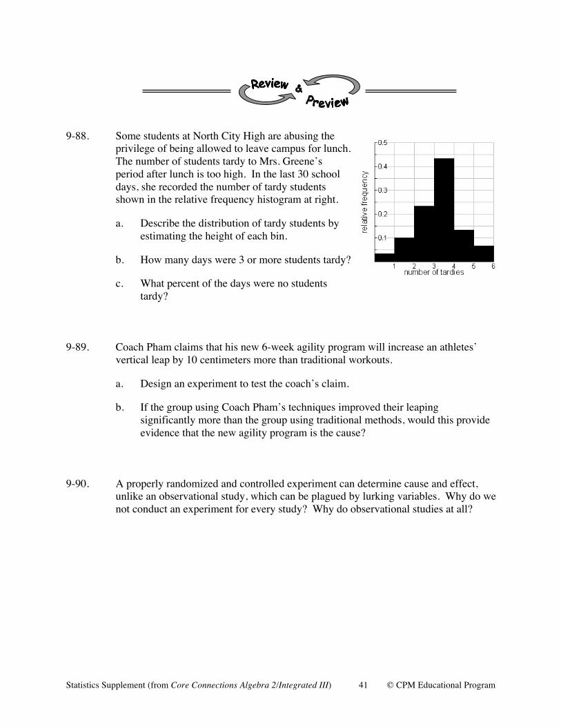
9-88. Some students at North City High are abusing the

privilege of being allowed to leave campus for lunch. The number of students tardy to Mrs. Greene’s period after lunch is too high. In the last 30 school days, she recorded the number of tardy students shown in the relative frequency histogram at right.

a. Describe the distribution of tardy students by estimating the height of each bin.

b. How many days were 3 or more students tardy?

c. What percent of the days were no students tardy?

9-89. Coach Pham claims that his new 6-week agility program will increase an athletes’

vertical leap by 10 centimeters more than traditional workouts.

a. Design an experiment to test the coach’s claim.

b. If the group using Coach Pham’s techniques improved their leaping significantly more than the group using traditional methods, would this provide evidence that the new agility program is the cause?

9-90. A properly randomized and controlled experiment can determine cause and effect,

unlike an observational study, which can be plagued by lurking variables. Why do we not conduct an experiment for every study? Why do observational studies at all?


9.3.3 How well did I do? • • • • • • • • • • • • • • • • • • • • • • • • • • • • • • • • • • • • • • • • • • • • • • • • • • • • • • • • • • • • • • • • • • • • • • • • • Percentiles 9-97. The ACT is a test that colleges use to help make admissions decisions for potential

students. Nationwide, the scores are normally distributed, with a mean score of 21 (out of a possible 36) and a standard deviation of 4.7.

a. Model the scores of all test takers on your calculator using a normal distribution. An appropriate value for the maximum of the relative frequency axis is 0.1.

b. Adèle scored 25 on the ACT. With your team, explore how well she did. Remember your normal distribution is a model for the bars of a histogram. Shade the “bars” (the area under the normal distribution) for all the scores below Adèle’s score. What percent of scores are below Adèle’s score? Round to the nearest whole number.

c. Since 80% of test-takers scored below Adèle, you can say that Adèle scored in the 80th percentile. Rémy scored a 16 on the ACT. What was Rémy’s percentile?

d. Antoinette scored 21 on the ACT. Without a calculator, make a sketch of the scores below Antoinette on a normal distribution and indicate what percentile Antoinette fell in.


9-98. Percentiles are not just for normal distributions. They can be used for any set of data to report the percent of scores that fell below a given score. The following data are the test scores on Mrs. Abraha’s Chapter 3 test in Geometry.

Chapter 3 Geometry Test Scores 75 86 94 89 80

72 17 94 56 80

91 71 79 57 94

90 58 60 93 75

83 86 53 93 92

60 81 89 94 69

89 86 42 76 75

checksum 2679

a. Make a histogram of the data on your calculator and sketch it. Use a bin width of 5.

b. Lateefa is modeling the data using a normal distribution, but her partner Farid thinks that it is not a good idea. What advice would you give them about using a normal distribution?

c. Lateefa scored 86 on the test, and Farid scored 92. What percentile did each score in?

d. What score is at the 25th percentile? 75th percentile?

e. Find the five number summary (minimum, first quartile, median, third quartile, maximum) for this data. How does your answer compare to part (d) above?

9-99. The March 2004 issue of Ichthyological Research

reported the relative frequencies for the length of 98 larvae of the ayu sweetfish is shown at right.

a. Estimate the 90th percentile for the length of ayu larvae.

b. Would you recommend making a model using a normal distribution for the data to answer part (a)? Why or why not?

c. Estimate the 50th percentile. What is another name for the 50th percentile?


9-100. Rachna’s physics class is going out to the football field to launch rockets today. The rocket that Rachna is launching has historically had a mean flight distance of 74 m with a standard deviation of 26 m. A rocket’s flight distance is modeled with a normal distribution.

a. Make a graph of the distribution of Rachna’s rocket flight distances on your calculator, and sketch it. An appropriate value for the maximum of the relative frequency axis is 0.02.

b. From your graph, visually estimate the two flight distances between which the rocket will land 90% of the time. Shade this portion of your sketch.

c. Use your calculator to check your estimate. How close to 90% did you come?

d. The middle 90% (or 95% or 99%) of the data is an important computation in statistics. It tells you what “typical” data might look like without considering the small or large extremes at either end. Statistical computations will reveal that the lower bound of the middle 90% of normally distributed data is at –1.6449 times the standard deviation, and the upper bound is at 1.6449 times the standard deviation. Use this new information to make a new, more accurate, determination of the two distances between which the rocket will land 90% of the time.

9-101. Rachna and her sister, Rakhi, were both in the same physics class. They made a bet

with each other on whose rocket would go farther. The loser would have to wash the family dishes for a month! Unfortunately, Rakhi was assigned a very different style rocket from the one Rachna got, so it was difficult to make a fair comparison. They decided to compare the percentiles. Rakhi’s style of rocket had a mean flight distance of 30 m with a standard deviation of 6 m.

Rachna’s rocket went 66.74 m, while Rakhi’s went 28.17 m. Use percentiles to

determine who had to wash the dishes for a month. 9-102. In response to a judging controversy during the 2002 Winter Olympics, a new scoring

system for ice dancing was implemented in 2006. The new system uses a “grade of execution” (GOE) as part of the overall score. The GOE goes from –3 to 3, and can be modeled with a normal distribution with mean of 0 and standard deviation of 1. Isabella and Tony scored a 2 on the GOE. What percentile are they in? What percentage of ice dancers had higher scores?


mean

total area = 1 (100%)

1 std deviation

For many situations in science, business, and industry, data may be represented by a bell-shaped curve. In order to be able to work mathematically with that data – describing it to others, making predictions – an equation called a normal probability density function is fitted to the data. This is very similar to how a line of best fit is used to describe and make predictions of data on a scatterplot.

The normal probability density function (“normal distribution”) stretches to infinity in both directions. The area under the normal distribution can be thought of as modeling the bars on a relative frequency histogram. However, instead of drawing all the bars, a curve is drawn that represents the tops of all the bars. Like bars on a relative frequency histogram, the area under the normal distribution (shaded in the diagram below) represents the portion of the population within that interval.

The total area under the curve is 1, representing 100% of the population. The mean of the population is at the peak of the normal distribution, resulting in 50% of the population below the mean and 50% above the mean.

The width of the normal distribution is determined by the standard deviation (the variability) of the population under study. The more variability in the data, the wider (and flatter) the normal distribution is.

MA

TH N

OTE

S ETHODS AND MEANINGS

MMEMEANINGS Normal Probability Density Function


9-103. North City High School has served the following number of lunches since the

beginning of the school year. The data has been sorted.

Number of lunches sold per day 576 584 594 595 603

605 606 613 618 630

632 636 640 640 652

660 661 663 665 666

671 671 675 677 678

689 695 698 703 721

723 738 745 755 774

774 785

checksum 24711

a. What are the mean and standard deviation number of lunches in the sample?

b. What is the five number summary of the distribution?

c. Make a relative frequency histogram of the number of lunches served. Use a scale from 560 to 800 lunches, with a bin width of 40 lunches. Sketch the histogram and label the height of each of the bins.

d. Describe the distribution. Make sure you consider the center, shape, spread, and outliers.

e. Using your histogram, determine the percent of days on which fewer than 600 lunches were sold.

f. Using the histogram, estimate the percent of days on which between 600 and 700 lunches were sold.


9-104. Do you remember the students tardy to Ms. Greene’s class? Now that you have investigated how to create and use a normal distribution, model the number of tardy students Ms. Greene actually recorded using a normal distribution. The data Mrs. Greene gathered for 30 days is shown in the table below.

Number of tardy students per day 2 1 2 3 5

4 3 3 0 3

3 3 1 2 3

3 4 2 3 3

4 3 3 2 4

2 2 3 5 1

checksum 82

a. On your calculator, recreate the relative frequency histogram for the number of tardy students that is shown in problem 9-88.

b. Find the mean and standard deviation of the number of tardy students.

c. On your calculator, model the data with a normal distribution by pressing o and entering y = normalpdf(X, mean, standard deviation). Sketch the model with the histogram.

d. According to your model, on what percentage of days were 4 people tardy? Shade this proportion on a new sketch of the model, and calculate the proportion using normalcdf(lower, upper, mean, standard deviation) on your calculator.

e. Assume that the last 30 days in Mrs. Greene’s class were representative of the 180 days in the whole school year. According to your model, how many days this year can Mrs. Greene expect 4 or more tardy students? Sketch the area representing these days on a new graph of the model.

9-105. Due to natural variability in manufacturing, a 12-ounce can of soda does not usually

hold exactly 12 ounces of soda. The quality control department at a soda factory allows cans to hold a little more or a little less. According to specifications, a soda-can filling machine must fill each can with a mean of 12 ounces of soda and a standard deviation of 0.33 ounces. Filling machines can often be modeled with a normal distribution.

a. Use your calculator to create a graph of a normal distribution using normalpdf. Sketch the graph. An appropriate value for the maximum of the relative frequency axis is Ymax = 1.5.

b. How often do you actually get a 12 oz can of soda containing more than 12 oz?

c. What percent of cans contain between 11.5 and 12.5 ounces of soda? Shade your diagram from part (a) to represent these bottles.

Documents

9.3.2 How can I make predictions? - Mrs. Seegmiller's Math …mrsseegmillersclassroom.weebly.com/uploads/2/4/1/0/... · · 2014-05-01How can I make predictions ... mean and standard