Embed Size (px)
Citation preview
96 Journal of Reviews on Global Economics, 2015, 4, 96-107
E-ISSN: 1929-7092/15 © 2015 Lifescience Global
Intervalling-Effect Bias and Competition Policy
Panagiotis N. Fotis1,*, Victoria Pekka-Oikonomou2 and Michael L. Polemis3
1General Directorate for Competition, Hellenic Competition Commission, Athens, Greece
2Department of Business Administration, University of Piraeus, Piraeus, Greece
3Department of Economics, University of Piraeus, Piraeus, Greece
Abstract: The purpose of this paper is twofold. First, it aims to investigate whether the security’s systematic risk beta estimates change as the infrequent trading phenomenon appears. Second, it attempts to provide useful insight on the
impact of mergers and acquisitions on competition policy. For this reason, we employ the models of Scholes and Williams (1977), Dimson (1979), Cohen et al. (1983a) and Maynes and Rumsey (1993) on a small stock exchange with thickly infrequent trading stocks. The empirical results reveal that for some securities the models employed by Scholes
and Williams (1977) and Cohen et al. (1983a) improve the biasness of the Ordinary Least Squares Market Model (Maynes and Rumsey, 1993). We argue that competitors gain while merged entities loose or at least do not gain from the clearness of the investigated mergers.
Keywords: Intervalling-effect bias, Beta risk measurement, Infrequent trading phenomenon, Mergers and
Acquisitions, Competition policy.
1. INTRODUCTION
The intervalling-effect bias in security’s beta
estimates denotes the sensitivity of the beta to the
length of the interval return (daily, monthly or yearly).
Empirically, estimated beta values are systematically
changed as the return interval is varied if Independent
and Identically Distributed (IID) additive assumption is
violated.1 The seminal paper examining intervalling-
effect bias is attributed to Fama (1970).
Scholes and Williams (1977) and Dimson (1979)
addressed the intervalling-effect bias slightly differently
and showed the bias in beta caused by infrequent
trading phenomenon. The latter appears when some
stocks do not trade daily in the stock exchange. In such
a case, the estimated variance and co-variance of the
stock performance is positively correlated with their
trade frequency.
The link between the security’s beta estimates and
inferences for competition policy has also been
explored in the literature. According to this link critical
role plays the movement of securities’ residuals during
the examined time interval which is affected by the
*Address correspondence to this author at the P. Ioakim 5, 121 32 Peristeri Attikis, Greece; Tel: + 30-210-5712588; Fax: + 30-210-5712588; E-mail: [email protected]
1Levhari and Levy (1977) proved that the expected value of the estimated beta
of aggressive stocks (beta greater than one) increases as the time interval increases and hence be over- estimated (a positive monotonicity outcome in time interval). The opposite happening for defensive stocks (Levy-Levhari hypothesis).
event under scrutiny (Event study methodology). If the
event constitutes an announcement or a notification of
Mergers & Acquisitions (M&As), a researcher has the
ability to inference potential anti or pro competitive
effects of the scrutinized M&As. Cox and Portes (1998)
portray a detailed clarification of the competitive
outcomes for M&As with infrequent trading
phenomenon.
In the literature there is a vast majority of articles
which deal with the above mentioned research areas.
In particular and regarding the intervalling-effect bias in
security’s beta estimates, Hong and Satchell (2014)
examine Capital Asset Pricing Model (CAPM) in which
errors are correlated with exogenous factors and
consider the evaluation of betas on current time. The
authors show, inter alia, that the intervalling effect bias
process produces extremely good results for short time
intervals and that beta estimates are monotonic to time
interval. Milonas and Rompotis (2013) show that small
cap Exchange Traded Funds (ETFs) have greater
betas than large cap ETFs, while Ordinary Least
Square (OLS) beta of all the ETFs increases as the
interval return is lengthened regardless of the degree of
capitalization.
The most commonly empirical models which are
dealing with infrequent trading phenomenon are
attributed to Cohen et al. (1983a) and the Market
Model by Maynes and Rumsey (1993). Armitage and
Brzeszczynski (2011) argue that OLS method tends to
overestimate the beta coefficients than the ARCH
models. Sercu, Vanderbroek and Vinaimont (2008) find
Intervalling-Effect Bias and Competition Policy Journal of Reviews on Global Economics, 2015, Vol. 4 97
that OLS exhibits the highest bias and lowest standard
errors, while the model proposed by Scholes and
Whilliams (1977) delivers the lowest bias and the
highest standard errors.
Diacogiannis and Makri (2008) examine with OLS
the intervalling effect bias for a number of thinly traded
securities on the Athens Stock Exchange (ASE) and
conclude that the bias appears.2 They also compare
the beta estimates which are derived from the Scholes
and Williams (1977), Cohen et al. (1983a) and Maynes
and Rumsey (1993) models and state that there are no
statistically significant differences between the mean
beta estimates.3
As it concerns the literature regarding the anti or pro
competitive effects of M&As, Rahim and Pok (2013)
use an event study methodology and explore the short
– run wealth effects of M&As announcements in
Malaysia during the period from 2001 to 2009. They
find positive market reactions for both targets and
bidding firms. Fotis and Polemis (2012a) find mixed
results by investigating the short – run effects of critical
mergers in Greece the last decade, while Fotis,
Polemis and Zevgolis (2011) examine 13 requested
derogations from suspension during the period 1995–
2008 by applying and assessing the results of three
different event study methodologies (market model,
mean adjusted return model and market adjusted
return model). They found that the average abnormal
and cumulative returns of the requested firms are
positive and statistical significant.
Furthermore, Duso, Gugler and Yurtoglou (2010)
infer that a long time window around the
announcement merger date (25 or 50 days prior to the
event) increases the ability to capture mergers’ ex -
post profitability by using accounting data (see also
Mueller 1980). Bharba (2008) infers that potential
targets of M&As experience a statistically significant
wealth gain estimated to 0.59% over the three day
event window, while Duso, Neven and Röller (2007)
and Aktas, de Bodt and Roll (2007) thoroughly
investigated the anti or pro competitive effects of M&As
under the European merger control regime.4
2For a definition of thinly traded securities see section 2.1 below.
3For a literature review prior to 2008 see Hong and Satchell (2014). See also
Davidson and Josev (2005), Wang and Jones (2005), Ho and Tsay (2001) and Daves, Ehrhardt and Kunkel (2000). 4For a literature review prior to 2007 see Fotis et al. (2011;74). Residual
analysis has also been used in the literature in other research areas. See for
This paper relates to the above mentioned strands
of the literature. Unlike other similar studies (Vazakides
2006; Diacogiannis and Makri 2008), it provides useful
insights on the impact of M&As on competition policy
by utilizing event study methodology and investigating
four critical phase-II M&As cleared by the Hellenic
Competition Commission (HCC) from 2006 to 2011.5
The novelty of this paper lies in the fact that a
variety of issues related to the intervalling effect bias is
thoroughly examined within a small market such as the
ASE, while this examination is conducted during its
evolution to maturity. The main reason for choosing the
ASE as our benchmark is that it can be characterised
as a small emerging market which during the examined
period it experienced a huge fall of share prices and
thus a considerable number of infrequent trading
securities have emerged.
The remainder of this paper is organized as follows.
Section 2 presents the sample selection and the
research methodology. Section 3 encapsulates the
main findings of our analysis, while section 4 concludes
the paper. In the Appendix we present the derivation of
the employed econometric models.
2. SAMPLE SELECTION AND MODEL SPECIFICATION
The sample consists of 22 companies listed in the
ASE (three merged entities and 19 competitors) that
were active in four phase-II M&As in Greece during the
period 2006-2011. The said M&As took place in the oil
and energy markets as well as in the paper and food
industries.6
The sample securities exhibit a thick infrequent
trading phenomenon. Following Barthdoly, Olson and
Peare (2007) this means that they trade more than 80
of trading days or an average of than four days per
week. Moreover, a medium traded security trades
between 40 - 80 and a thin traded security trades less
than 40 days per year.
We utilise the models proposed by Scholes and
Williams (1977), Dimson (1979), Cohen et al. (1983a)
instance Gleason, Pennathur and Wiggenhorn (2014), Al-Sharkas and Hassan (2010) and Jiang and Leger (2010). An application of residual analysis on antitrust and abuse of dominant position can be found, inter alia, in Fotis (2012). Fotis (2014) explores the unilateral effects of M&As on competition by using UPP and GUPPI analysis. 5Phase – II M&As require an in depth investigation by the General Directorate
for Competition of HCC. 6The data are available from the authors upon request.
98 Journal of Reviews on Global Economics, 2015, Vol. 4 Fotis et al.
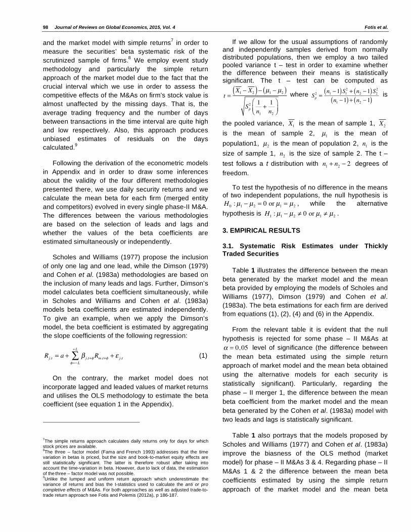
and the market model with simple returns7 in order to
measure the securities’ beta systematic risk of the
scrutinized sample of firms.8 We employ event study
methodology and particularly the simple return
approach of the market model due to the fact that the
crucial interval which we use in order to assess the
competitive effects of the M&As on firm’s stock value is
almost unaffected by the missing days. That is, the
average trading frequency and the number of days
between transactions in the time interval are quite high
and low respectively. Also, this approach produces
unbiased estimates of residuals on the days
calculated.9
Following the derivation of the econometric models
in Appendix and in order to draw some inferences
about the validity of the four different methodologies
presented there, we use daily security returns and we
calculate the mean beta for each firm (merged entity
and competitors) evolved in every single phase-II M&A.
The differences between the various methodologies
are based on the selection of leads and lags and
whether the values of the beta coefficients are
estimated simultaneously or independently.
Scholes and Williams (1977) propose the inclusion
of only one lag and one lead, while the Dimson (1979)
and Cohen et al. (1983a) methodologies are based on
the inclusion of many leads and lags. Further, Dimson’s
model calculates beta coefficient simultaneously, while
in Scholes and Williams and Cohen et al. (1983a)
models beta coefficients are estimated independently.
To give an example, when we apply the Dimson’s
model, the beta coefficient is estimated by aggregating
the slope coefficients of the following regression:
Rj ,t = a + j ,t+ Rm,t+= L
+L
+ j ,t (1)
On the contrary, the market model does not
incorporate lagged and leaded values of market returns
and utilises the OLS methodology to estimate the beta
coefficient (see equation 1 in the Appendix).
7The simple returns approach calculates daily returns only for days for which
stock prices are available. 8The three – factor model (Fama
and
French 1993)
addresses that the time
variation in betas is priced, but the size and book-to-market equity effects are
still statistically significant. The latter is therefore robust after taking into account the time-variation in beta. However, due
to lack of data, the estimation
of the three – factor model was not possible.
9Unlike the lumped and uniform return approach which underestimate the
variance of returns and bias the t-statistics used to calculate the anti or pro completive effects of M&As. For both approaches as well as adjusted trade-to-trade return approach see Fotis and Polemis (2012a), p 186-187.
If we allow for the usual assumptions of randomly and independently samples derived from normally distributed populations, then we employ a two tailed pooled variance t – test in order to examine whether the difference between their means is statistically significant. The t – test can be computed as
t =X1 X2( ) μ1 μ2( )
Sp2 1
n1+1
n2
where Sp2=
n1 1( )S12+ n2 1( )S2
2
n1 1( ) + n2 1( ) is
the pooled variance, X1 is the mean of sample 1, X2
is the mean of sample 2, μ1 is the mean of
population1, μ2 is the mean of population 2, n1 is the
size of sample 1, n2 is the size of sample 2. The t –
test follows a t distribution with n1 + n2 2 degrees of
freedom.
To test the hypothesis of no difference in the means of two independent populations, the null hypothesis is
H 0 :μ1 μ2 = 0 or μ1 = μ2 , while the alternative
hypothesis is H1 :μ1 μ2 0 or μ1 μ2 .
3. EMPIRICAL RESULTS
3.1. Systematic Risk Estimates under Thickly Traded Securities
Table 1 illustrates the difference between the mean
beta generated by the market model and the mean
beta provided by employing the models of Scholes and
Williams (1977), Dimson (1979) and Cohen et al.
(1983a). The beta estimations for each firm are derived
from equations (1), (2), (4) and (6) in the Appendix.
From the relevant table it is evident that the null
hypothesis is rejected for some phase – II M&As at
= 0, 05 level of significance (the difference between
the mean beta estimated using the simple return
approach of market model and the mean beta obtained
using the alternative models for each security is
statistically significant). Particularly, regarding the
phase – II merger 1, the difference between the mean
beta coefficient from the market model and the mean
beta generated by the Cohen et al. (1983a) model with
two leads and lags is statistically significant.
Table 1 also portrays that the models proposed by
Scholes and Williams (1977) and Cohen et al. (1983a)
improve the biasness of the OLS method (market
model) for phase – II M&As 3 & 4. Regarding phase – II
M&As 1 & 2 the difference between the mean beta
coefficients estimated by using the simple return
approach of the market model and the mean beta
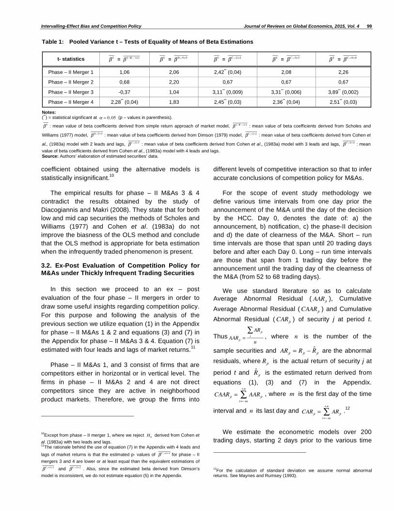
Intervalling-Effect Bias and Competition Policy Journal of Reviews on Global Economics, 2015, Vol. 4 99
coefficient obtained using the alternative models is
statistically insignificant.10
The empirical results for phase – II M&As 3 & 4
contradict the results obtained by the study of
Diacogiannis and Makri (2008). They state that for both
low and mid cap securities the methods of Scholes and
Williams (1977) and Cohen et al. (1983a) do not
improve the biasness of the OLS method and conclude
that the OLS method is appropriate for beta estimation
when the infrequently traded phenomenon is present.
3.2. Ex-Post Evaluation of Competition Policy for M&As under Thickly Infrequent Trading Securities
In this section we proceed to an ex – post
evaluation of the four phase – II mergers in order to
draw some useful insights regarding competition policy.
For this purpose and following the analysis of the
previous section we utilize equation (1) in the Appendix
for phase – II M&As 1 & 2 and equations (3) and (7) in
the Appendix for phase – II M&As 3 & 4. Equation (7) is
estimated with four leads and lags of market returns.11
Phase – II M&As 1, and 3 consist of firms that are
competitors either in horizontal or in vertical level. The
firms in phase – II M&As 2 and 4 are not direct
competitors since they are active in neighborhood
product markets. Therefore, we group the firms into
10Except from phase – II merger 1, where we reject H0 derived from Cohen et
al. (1983a) with two leads and lags. 11
The rationale behind the use of equation (7) in the Appendix with 4 leads and
lags of market returns is that the estimated p- values of C , 4+4 for phase – II
mergers 3 and 4 are lower or at least equal than the equivalent estimations of
C , 3+3 and C , 2+2 . Also, since the estimated beta derived from Dimson’s
model is inconsistent, we do not estimate equation (5) in the Appendix.
different levels of competitive interaction so that to infer
accurate conclusions of competition policy for M&As.
For the scope of event study methodology we
define various time intervals from one day prior the
announcement of the M&A until the day of the decision
by the HCC. Day 0, denotes the date of: a) the
announcement, b) notification, c) the phase-II decision
and d) the date of clearness of the M&A. Short – run
time intervals are those that span until 20 trading days
before and after each Day 0. Long – run time intervals
are those that span from 1 trading day before the
announcement until the trading day of the clearness of
the M&A (from 52 to 68 trading days).
We use standard literature so as to calculate
Average Abnormal Residual ( AARjt ), Cumulative
Average Abnormal Residual (CAARjt ) and Cumulative
Abnormal Residual (CARjt ) of security j at period t.
Thus AARjt =
ARjtj
n, where n is the number of the
sample securities and ARjt = Rjt R̂jt are the abnormal
residuals, where Rjt is the actual return of security j at
period t and R̂jt is the estimated return derived from
equations (1), (3) and (7) in the Appendix.
CAARjt = AARjtt= m
+n
, where m is the first day of the time
interval and n its last day and CARjt = ARjtt= m
+n
.12
We estimate the econometric models over 200
trading days, starting 2 days prior to the various time
12For the calculation of standard deviation we assume normal abnormal
returns. See Maynes and Rumsey (1993).
Table 1: Pooled Variance t – Tests of Equality of Means of Beta Estimations
t- statistics S = S W , 1+1 S = D, 5+5 S = C , 2+2 S = C , 3+3 S = C , 4+4
Phase – II Merger 1 1,06 2,06 2,42** (0,04) 2,08 2,26
Phase – II Merger 2 0,68 2,20 0,67 0,67 0,67
Phase – II Merger 3 -0,37 1,04 3,11** (0,009) 3,31
** (0,006) 3,89
** (0,002)
Phase – II Merger 4 2,28** (0,04) 1,83 2,45
** (0,03) 2,36
** (0,04) 2,51
** (0,03)
Notes: (**) = statistical significant at = 0, 05 (p – values in parenthesis).
S : mean value of beta coefficients derived from simple return approach of market model, S W , 1+1 : mean value of beta coefficients derived from Scholes and
Williams (1977) model, D, 5+5 : mean value of beta coefficients derived from Dimson (1979) model, C , 2+2 : mean value of beta coefficients derived from Cohen et
al., (1983a) model with 2 leads and lags, C , 3+3 : mean value of beta coefficients derived from Cohen et al., (1983a) model with 3 leads and lags, C , 4+4 : mean
value of beta coefficients derived from Cohen et al., (1983a) model with 4 leads and lags. Source: Authors’ elaboration of estimated securities’ data.
100 Journal of Reviews on Global Economics, 2015, Vol. 4 Fotis et al.
intervals. For simple return approach of market model
the estimation interval of the econometric models is
greater than a calendar year.
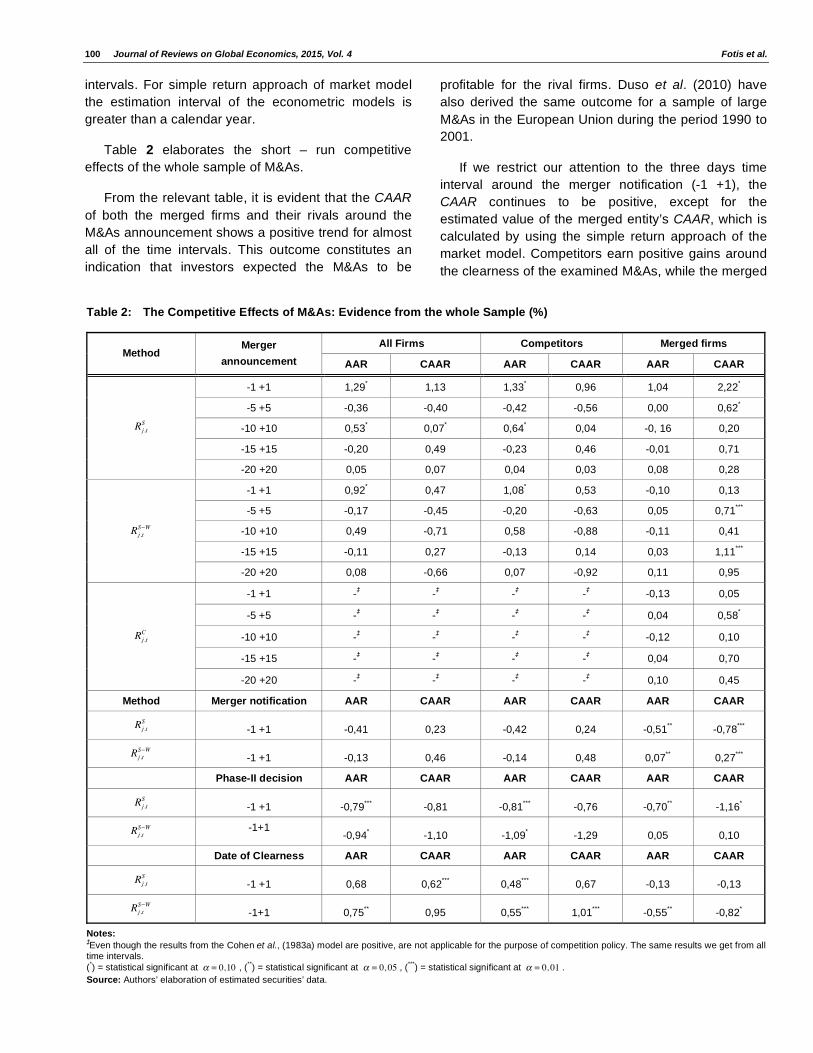
Table 2 elaborates the short – run competitive
effects of the whole sample of M&As.
From the relevant table, it is evident that the CAAR
of both the merged firms and their rivals around the
M&As announcement shows a positive trend for almost
all of the time intervals. This outcome constitutes an
indication that investors expected the M&As to be
profitable for the rival firms. Duso et al. (2010) have
also derived the same outcome for a sample of large
M&As in the European Union during the period 1990 to
2001.
If we restrict our attention to the three days time
interval around the merger notification (-1 +1), the
CAAR continues to be positive, except for the
estimated value of the merged entity’s CAAR, which is
calculated by using the simple return approach of the
market model. Competitors earn positive gains around
the clearness of the examined M&As, while the merged
Table 2: The Competitive Effects of M&As: Evidence from the whole Sample (%)
All Firms Competitors Merged firms Method
Merger
announcement AAR CAAR AAR CAAR AAR CAAR
-1 +1 1,29* 1,13 1,33
* 0,96 1,04 2,22
*
-5 +5 -0,36 -0,40 -0,42 -0,56 0,00 0,62*
-10 +10 0,53* 0,07
* 0,64
* 0,04 -0, 16 0,20
-15 +15 -0,20 0,49 -0,23 0,46 -0,01 0,71
Rj ,tS
-20 +20 0,05 0,07 0,04 0,03 0,08 0,28
-1 +1 0,92* 0,47 1,08
* 0,53 -0,10 0,13
-5 +5 -0,17 -0,45 -0,20 -0,63 0,05 0,71***
-10 +10 0,49 -0,71 0,58 -0,88 -0,11 0,41
-15 +15 -0,11 0,27 -0,13 0,14 0,03 1,11***
Rj ,tS W
-20 +20 0,08 -0,66 0,07 -0,92 0,11 0,95
-1 +1 -‡ -
‡ -
‡ -
‡ -0,13 0,05
-5 +5 -‡ -
‡ -
‡ -
‡ 0,04 0,58
*
-10 +10 -‡ -
‡ -
‡ -
‡ -0,12 0,10
-15 +15 -‡ -
‡ -
‡ -
‡ 0,04 0,70
Rj ,tC
-20 +20 -‡ -
‡ -
‡ -
‡ 0,10 0,45
Method Merger notification AAR CAAR AAR CAAR AAR CAAR
Rj ,tS -1 +1 -0,41 0,23 -0,42 0,24 -0,51
** -0,78
***
Rj ,tS W -1 +1 -0,13 0,46 -0,14 0,48 0,07
** 0,27
***
Phase-II decision AAR CAAR AAR CAAR AAR CAAR
Rj ,tS -1 +1 -0,79
*** -0,81 -0,81
*** -0,76 -0,70
** -1,16
*
Rj ,tS W -1+1
-0,94* -1,10 -1,09
* -1,29 0,05 0,10
Date of Clearness AAR CAAR AAR CAAR AAR CAAR
Rj ,tS -1 +1 0,68 0,62
*** 0,48
*** 0,67 -0,13 -0,13
Rj ,tS W -1+1 0,75
** 0,95 0,55
*** 1,01
*** -0,55
** -0,82
*
Notes: ‡Even though the results from the Cohen et al., (1983a) model are positive, are not applicable for the purpose of competition policy. The same results we get from all time intervals.
(*) = statistical significant at = 0,10 , (
**) = statistical significant at = 0, 05 , (
***) = statistical significant at = 0, 01 .
Source: Authors’ elaboration of estimated securities’ data.
Intervalling-Effect Bias and Competition Policy Journal of Reviews on Global Economics, 2015, Vol. 4 101
entities loose. However, the decrease of the merged
entities’ security value does not offset their highly
significant positive gains during the three days interval
around the announcement of the merger. The positive
trend of firms’ residuals constitutes an indication that
the market is concerned about their possibly anti
competitive effects.
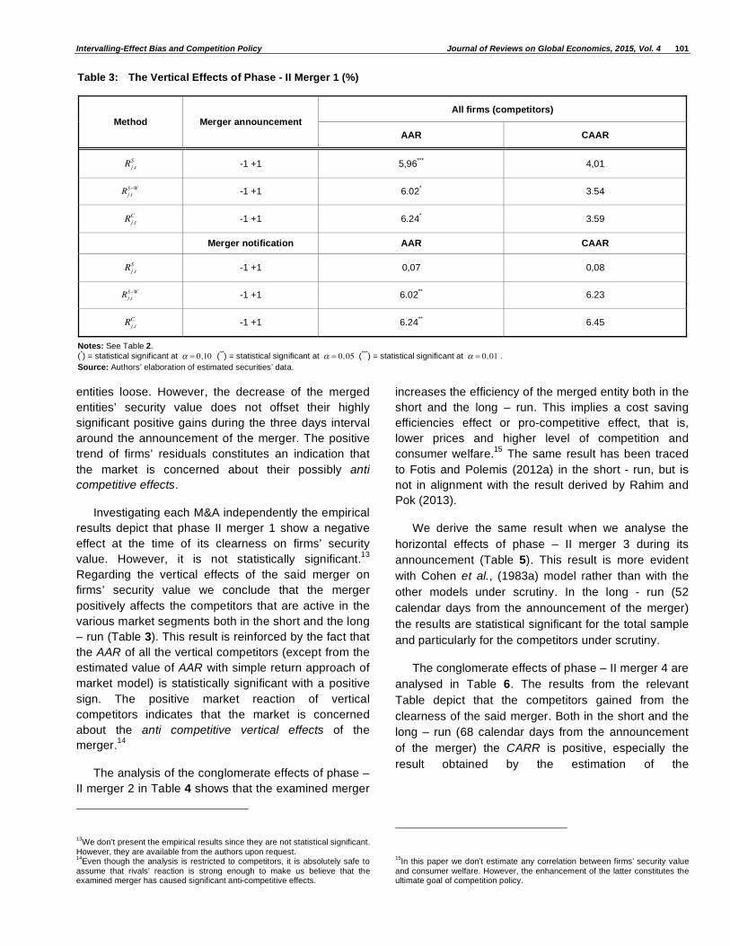
Investigating each M&A independently the empirical
results depict that phase II merger 1 show a negative
effect at the time of its clearness on firms’ security
value. However, it is not statistically significant.13
Regarding the vertical effects of the said merger on
firms’ security value we conclude that the merger
positively affects the competitors that are active in the
various market segments both in the short and the long
– run (Table 3). This result is reinforced by the fact that
the AAR of all the vertical competitors (except from the
estimated value of AAR with simple return approach of
market model) is statistically significant with a positive
sign. The positive market reaction of vertical
competitors indicates that the market is concerned
about the anti competitive vertical effects of the
merger.14
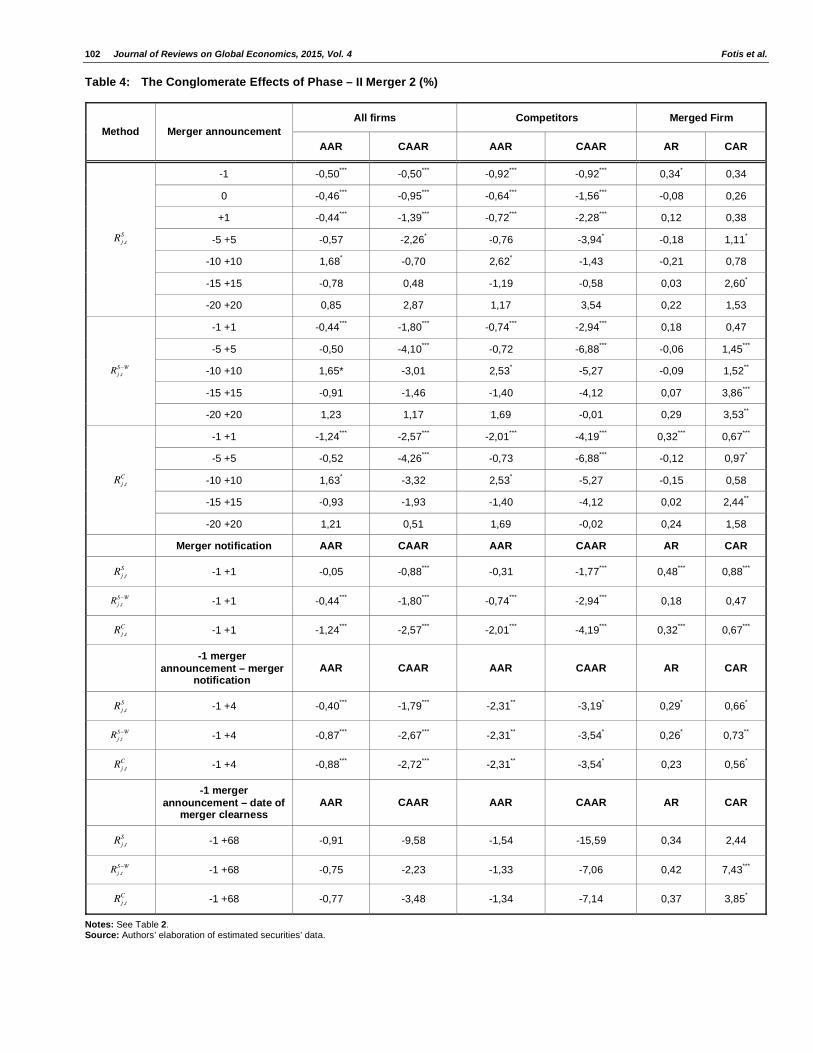
The analysis of the conglomerate effects of phase –
II merger 2 in Table 4 shows that the examined merger
13We don’t present the empirical results since they are not statistical significant.
However, they are available from the authors upon request. 14
Even though the analysis is restricted to competitors, it is absolutely safe to assume that rivals’ reaction is strong enough to make us believe that the examined merger has caused significant anti-competitive effects.
increases the efficiency of the merged entity both in the
short and the long – run. This implies a cost saving
efficiencies effect or pro-competitive effect, that is,
lower prices and higher level of competition and
consumer welfare.15
The same result has been traced
to Fotis and Polemis (2012a) in the short - run, but is
not in alignment with the result derived by Rahim and
Pok (2013).
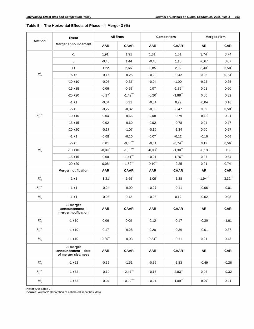
We derive the same result when we analyse the
horizontal effects of phase – II merger 3 during its
announcement (Table 5). This result is more evident
with Cohen et al., (1983a) model rather than with the
other models under scrutiny. In the long - run (52
calendar days from the announcement of the merger)
the results are statistical significant for the total sample
and particularly for the competitors under scrutiny.
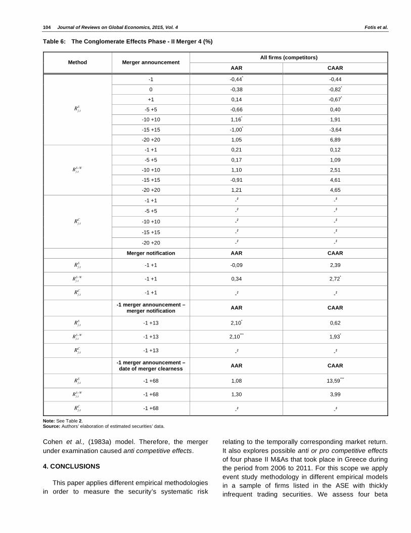
The conglomerate effects of phase – II merger 4 are
analysed in Table 6. The results from the relevant
Table depict that the competitors gained from the
clearness of the said merger. Both in the short and the
long – run (68 calendar days from the announcement
of the merger) the CARR is positive, especially the
result obtained by the estimation of the
15In this paper we don’t estimate any correlation between firms’ security value
and consumer welfare. However, the enhancement of the latter constitutes the ultimate goal of competition policy.
Table 3: The Vertical Effects of Phase - II Merger 1 (%)
All firms (competitors)
Method Merger announcement
AAR CAAR
Rj ,tS -1 +1 5,96
*** 4,01
Rj ,tS W -1 +1 6.02
* 3.54
Rj ,tC -1 +1 6.24
* 3.59
Merger notification AAR CAAR
Rj ,tS -1 +1 0,07 0,08
Rj ,tS W -1 +1 6.02
** 6.23
Rj ,tC -1 +1 6.24
** 6.45
Notes: See Table 2.
(*) = statistical significant at = 0,10 (
**) = statistical significant at = 0, 05 (
***) = statistical significant at = 0, 01 .
Source: Authors’ elaboration of estimated securities’ data.
102 Journal of Reviews on Global Economics, 2015, Vol. 4 Fotis et al.
Table 4: The Conglomerate Effects of Phase – II Merger 2 (%)
All firms Competitors Merged Firm
Method Merger announcement
AAR CAAR AAR CAAR AR CAR
-1 -0,50***
-0,50***
-0,92***
-0,92***
0,34* 0,34
0 -0,46***
-0,95***
-0,64***
-1,56***
-0,08 0,26
+1 -0,44***
-1,39***
-0,72***
-2,28***
0,12 0,38
-5 +5 -0,57 -2,26* -0,76 -3,94
* -0,18 1,11
*
-10 +10 1,68* -0,70 2,62
* -1,43 -0,21 0,78
-15 +15 -0,78 0,48 -1,19 -0,58 0,03 2,60*
Rj ,tS
-20 +20 0,85 2,87 1,17 3,54 0,22 1,53
-1 +1 -0,44***
-1,80***
-0,74***
-2,94***
0,18 0,47
-5 +5 -0,50 -4,10***
-0,72 -6,88***
-0,06 1,45***
-10 +10 1,65* -3,01 2,53* -5,27 -0,09 1,52
**
-15 +15 -0,91 -1,46 -1,40 -4,12 0,07 3,86***
Rj ,tS W
-20 +20 1,23 1,17 1,69 -0,01 0,29 3,53**
-1 +1 -1,24***
-2,57***
-2,01***
-4,19***
0,32***
0,67***
-5 +5 -0,52 -4,26***
-0,73 -6,88***
-0,12 0,97*
-10 +10 1,63* -3,32 2,53
* -5,27 -0,15 0,58
-15 +15 -0,93 -1,93 -1,40 -4,12 0,02 2,44**
Rj ,tC
-20 +20 1,21 0,51 1,69 -0,02 0,24 1,58
Merger notification AAR CAAR AAR CAAR AR CAR
Rj ,tS -1 +1 -0,05 -0,88
*** -0,31 -1,77
*** 0,48
*** 0,88
***
Rj ,tS W -1 +1 -0,44
*** -1,80
*** -0,74
*** -2,94
*** 0,18 0,47
Rj ,tC -1 +1 -1,24
*** -2,57
*** -2,01
*** -4,19
*** 0,32
*** 0,67
***
-1 merger
announcement – merger notification
AAR CAAR AAR CAAR AR CAR
Rj ,tS -1 +4 -0,40
*** -1,79
*** -2,31
** -3,19
* 0,29
* 0,66
*
Rj ,tS W -1 +4 -0,87
*** -2,67
*** -2,31
** -3,54
* 0,26
* 0,73
**
Rj ,tC -1 +4 -0,88
*** -2,72
*** -2,31
** -3,54
* 0,23 0,56
*
-1 merger
announcement – date of merger clearness
AAR CAAR AAR CAAR AR CAR
Rj ,tS -1 +68 -0,91 -9,58 -1,54 -15,59 0,34 2,44
Rj ,tS W -1 +68 -0,75 -2,23 -1,33 -7,06 0,42 7,43
***
Rj ,tC -1 +68 -0,77 -3,48 -1,34 -7,14 0,37 3,85
*
Notes: See Table 2. Source: Authors’ elaboration of estimated securities’ data.
Intervalling-Effect Bias and Competition Policy Journal of Reviews on Global Economics, 2015, Vol. 4 103
Table 5: The Horizontal Effects of Phase – II Merger 3 (%)
All firms Competitors Merged Firm
Method Event
Merger announcement AAR CAAR AAR CAAR AR CAR
-1 1,91* 1,91 1,61
* 1,61 3,74
* 3,74
0 -0,48 1,44 -0,45 1,16 -0,67 3,07
+1 1,22 2,66* 0,85 2,02 3,43
* 6,50
*
-5 +5 -0,16 -0,25 -0,20 -0,42 0,05 0,73*
-10 +10 -0,07 -0,82* -0,04 -1,00
* -0,25
* 0,25
-15 +15 0,06 -0,99* 0,07 -1,25
** 0,01 0,60
Rj ,tS
-20 +20 -0,17* -1,49
*** -0,20
* -1,88
*** 0,00 0,82
-1 +1 -0,04 0,21 -0,04 0,22 -0,04 0,16
-5 +5 -0,27 -0,32 -0,33 -0,47 0,09 0,58*
-10 +10 0,04 -0,65 0,08 -0,79 -0,18* 0,21
-15 +15 0,02 -0,60 0,02 -0,78 0,04 0,47
Rj ,tS W
-20 +20 -0,17 -1,07 -0,19 -1,34 0,00 0,57
-1 +1 -0,08* -0,10 -0,07
* -0,12
* -0,10 0,06
-5 +5 0,01 -0,56***
-0,01 -0,74***
0,12 0,56*
-10 +10 -0,09** -1,06
*** -0,08
** -1,30
*** -0,13 0,36
-15 +15 0,00 -1,41***
-0,01 -1,76***
0,07 0,64
Rj ,tC
-20 +20 -0,08** -1,82
*** -0,10
*** -2,25 0,01 0,74
*
Merger notification AAR CAAR AAR CAAR AR CAR
Rj ,tS -1 +1 -1,21
* -1,66
* -1,09
* -1,38 -1,94
*** -3,31
***
Rj ,tS W -1 +1 -0,24 -0,09 -0,27 -0,11 -0,06 -0,01
Rj ,tC -1 +1 -0,06 0,12 -0,06 0,12 -0,02 0,08
-1 merger
announcement – merger notification
AAR CAAR AAR CAAR AR CAR
Rj ,tS -1 +10 0,06 0,09 0,12 -0,17 -0,30 -1,61
Rj ,tS W -1 +10 0,17 -0,28 0,20 -0,39 -0,01 0,37
Rj ,tC -1 +10 0,20
** -0,03 0,24
** -0,11 0,01 0,43
-1 merger
announcement – date of merger clearness
AAR CAAR AAR CAAR AR CAR
Rj ,tS -1 +52 -0,35 -1,61 -0,32 -1,83 -0,49 -0,26
Rj ,tS W -1 +52 -0,10 -2,47
*** -0,13 -2,83
*** 0,06 -0,32
Rj ,tC -1 +52 -0,04 -0,90
*** -0,04 -1,09
*** -0,07
* 0,21
Note: See Table 2. Source: Authors’ elaboration of estimated securities’ data.
104 Journal of Reviews on Global Economics, 2015, Vol. 4 Fotis et al.
Table 6: The Conglomerate Effects Phase - II Merger 4 (%)
All firms (competitors) Method Merger announcement
AAR CAAR
-1 -0,44* -0,44
0 -0,38 -0,82*
+1 0,14 -0,67*
-5 +5 -0,66 0,40
-10 +10 1,16* 1,91
-15 +15 -1,00* -3,64
Rj ,tS
-20 +20 1,05 6,89
-1 +1 0,21 0,12
-5 +5 0,17 1,09
-10 +10 1,10 2,51
-15 +15 -0,91 4,61
Rj ,tS W
-20 +20 1,21 4,65
-1 +1 -‡ -
‡
-5 +5 -‡ -
‡
-10 +10 -‡ -
‡
-15 +15 -‡ -
‡
Rj ,tC
-20 +20 -‡ -
‡
Merger notification AAR CAAR
Rj ,tS -1 +1 -0,09 2,39
Rj ,tS W -1 +1 0,34 2,72
*
Rj ,tC -1 +1 -
‡ -
‡
-1 merger announcement –
merger notification AAR CAAR
Rj ,tS -1 +13 2,10
* 0,62
Rj ,tS W -1 +13 2,10
*** 1,93
*
Rj ,tC -1 +13 -
‡ -
‡
-1 merger announcement – date of merger clearness
AAR CAAR
Rj ,tS -1 +68 1,08 13,59
***
Rj ,tS W -1 +68 1,30 3,99
Rj ,tC -1 +68 -
‡ -
‡
Note: See Table 2. Source: Authors’ elaboration of estimated securities’ data.
Cohen et al., (1983a) model. Therefore, the merger
under examination caused anti competitive effects.
4. CONCLUSIONS
This paper applies different empirical methodologies
in order to measure the security’s systematic risk
relating to the temporally corresponding market return.
It also explores possible anti or pro competitive effects
of four phase II M&As that took place in Greece during
the period from 2006 to 2011. For this scope we apply
event study methodology in different empirical models
in a sample of firms listed in the ASE with thickly
infrequent trading securities. We assess four beta
Intervalling-Effect Bias and Competition Policy Journal of Reviews on Global Economics, 2015, Vol. 4 105
evaluating models developed by Scholes and Williams
(1977), Dimson (1979), Cohen et al. (1983a) and
Maynes and Rumsey (1993).
he empirical results indicate that the models by
Scholes and Williams (1977) and Cohen et al. (1983a)
improve the biasness raised from the application of the
OLS method. It is worth mentioning that, when we use
the Dimson’s methodology the difference between the
estimated betas is not statistically significant.
The applied ex post evaluation of competition policy
in the whole sample depicts that competitors gain while
merged entities loose (or at least do not gain) from the
clearness of the scrutinized M&As in the short - run.
This result indicates decreased efficiency for the
merged firms and enhanced profitability for the
competitors.
However, if we focus our attention on each
individual phase – II M&A, the results are rather
controversial. More specifically, phase – II merger 1
positively affects competitors that are active in different
levels of production in the short – run (vertical anti
competitive effects), while phase – II M&As 2 & 3
positively affect the level of competition in the relevant
product markets both in the short and long – run
(conglomerate and horizontal pro competitive effects
correspondingly). Moreover, the clearness of phase – II
conglomerate merger 4 restricts the level of
competition in the relevant product markets.
ACKNOWLEDGEMENT
This paper benefits from the valuable comments of
the participants of the 1st International Conference of
Business and Economics, Hellenic Open University, 6-
7 February, Athens, Greece. We are solely responsible
for its errors.
APPENDIX
Derivation of econometric models
Following Maynes and Rumsey (1993), Fotis et al. (2011) and Fotis and Polemis (2012a) the market model forecasts that firm j’s security simple return at
time t ( Rj ,tS ) is proportional to a market return. That is,
RjtS= a + SRm,t + jt (1)
where Rmt is the return on the market index for the day t
and s the beta coefficient of simple return market
model.
Scholes and Williams (1977) have indicated that
beta coefficients are downward biased for infrequently
traded securities and they are upward biased for very
frequently traded securities. They proposed a
consistent estimator of beta which is given by equation
(2):
S W=
jt1+ jt
0+ jt
+1
(1+ 2 mt ) (2)
where jt1 , jt
0 and jt+1 are estimates of beta
coefficient from the regression between the observed security return and market index return at
t = 1, t = 0 and t = +1 respectively and mt is the first-
order serial correlation coefficient of market returns.
Given equations (1) and (2), the market model becomes,
RjtS W
= a + S W Rmt + jt (3)
Dimson (1979) advocates that the return on a
specific security depends on past, present and future
returns of the market portfolio. Dimson’s beta
coefficient is given in equation (4):
D= jt+
= L
+L
(4)
where = L......+ L are lagged, contemporaneous
and leading estimated values of beta coefficient. Substituting equation (4) into equation (1), we calculate
firm j’s security return at time t ( RjtD ):
RjtD= a + DRmt + jt (5)
The Cohen et al. (1983a) model (see also Cohen et
al. (1983b), as opposed to the Scholes and Williams
(1977) models, utilizes many leads and lags of the
market portfolio’s return so as to produce an efficient
beta coefficient. Cohen et al. (1983a) and Fowler and
Rorke (1983) argue that the beta estimator of Dimson’s
model generates inconsistent estimates. Cohen et al.
(1983a) proposed a consistent estimator, which is
given by equation (6):
C=
jt + jt+L + jt L=1
L
=1
L
(1+ mt+L + mt L=1
L
=1
L
) (6)
where mt+L and mt L are the L – order serial
correlation of market portfolio’s returns and L, + L

106 Journal of Reviews on Global Economics, 2015, Vol. 4 Fotis et al.
imply lagged and leading values of L . Substituting equation (6) into equation (1), we calculate firm j’s
security return at time t ( RjtC ):
RjtC= a + CRmt + jt (7)
REFERENCES
Armitage Seth and Janusz Brzeszczynski. 2011. “Heteroscedasticity and Interval Effects in Estimating Beta: UK Evidence.”
Applied Financial Economics 21(20):1525-1538. http://dx.doi.org/10.1080/09603107.2011.581208
Aktas, Nihat, Eric de Bodt and Richard Roll. 2007. “European M&A Regulation is Protectionist.” The Economic Journal
117:1096–1121. http://dx.doi.org/10.1111/j.1468-0297.2007.02068.x
Al-Sharkas, Adel A and Kabir M Hassan. 2010. “New Evidence on Shareholder Wealth Effects in Bank Mergers during 1980-2000.” Journal of Economics and Finance 34(3):326-348. http://dx.doi.org/10.1007/s12197-008-9071-1
Barthodly, Jan, Dennis Olson and Paula Peare. 2007. “Conducting Event Studies on a Small Stock Exchange.” The European Journal of Finance 13(3):227-252. http://dx.doi.org/10.1080/13518470600880176
Bharba Gurmeet Singh. 2008. “Potential Targets: An Analysis of
Stock Price Reaction to Acquisition Program Announcements.” Journal of Economics and Finance 2(2):158-175.
Cohen, J Kalman, Gabriel A Hawawini, Steven F Maier, Robert A
Schwartz, and David K Whitcomb. 1983b. “Estimating and Adjusting for the Intervalling- Effect Bias in Beta.” Managerial Science 29:135- 148. http://dx.doi.org/10.1287/mnsc.29.1.135
Cohen, J Kalman, Gabriel A Hawawini, Steven F Maier, Robert A
Schwartz, and David K Whitcomb. 1983a. “Friction in the Trading Process and the Estimation of Systematic Risk.” Journal of Economics and Finance 12:263- 278. http://dx.doi.org/10.1016/0304-405X(83)90038-7
Cox, J Alan. and Jonathan Portes. 1998. “Mergers in Regulated
Industries: The Uses and Abuses of Event Studies.” Journal of Regulation and Economics 14:281-285. http://dx.doi.org/10.1023/A:1008087424850
Daves, R Phillip, Michael C Ehrhardt, and Robert A Kunkel. 2000.
“Estimating Systematic Risk: The Choice of Return Iinterval and Estimation Period.” Journal of Financial and Strategic Decisions 13:7-13.
Davidson Sinclair and Thomas Josev. 2005. “The Impact of Thin Trading Adjustments on Australian Beta Estimates.”
Accounting Research Journal 18(2):111 – 117. http://dx.doi.org/10.1108/10309610580000679
Diacogiannis George and Paraskevi Makri. 2008. “Estimating Betas in Thinner Markets: The Case of the Athens Stock Exchange.” International Research Journal of Finance and
Economics 13:108-122.
Dimson Elroy. 1979. “Risk Measurement when Shares are Subject to
Infrequent Trading.” Journal of Financial Economics 7:197-226. http://dx.doi.org/10.1016/0304-405X(79)90013-8
Duso, Tomaso, Damien J Neven and Lars-Hendrik Röller. 2007. “The Political Economy of European Merger Control: Evidence
Using Stock Market Data.” Journal of Law and Economics 50(3):455-489. http://dx.doi.org/10.1086/519812
Duso, Tomaso, Klaus Gugler and Burcin Yurtoglou. 2010. “Is the Event Study Methodology Useful for Merger Analysis? A
Comparison of Stock Market and Accounting Data.” International Review of Law and Economics 30:186-192. http://dx.doi.org/10.1016/j.irle.2010.02.001
Fama F Eugene. 1970. “The Behavior of Stock Market Prices.”
Journal of Business 38:34-105. http://dx.doi.org/10.1086/294743
Fama F Eugene and Kenneth R French. 1993. “Common risk factors in the returns on stocks and bonds.” Journal of Financial Economics 33:3-56. http://dx.doi.org/10.1016/0304-405X(93)90023-5
Fotis, Panagiotis. 2012. “Competition Policy & Firm’s Damages.” Pp. 116-139 in Recent Advances in the Analysis of Competition Policy and Regulation, edited by Y. Katsulakos and J. E.
Harrington, London UK. http://dx.doi.org/10.4337/9781781005699.00012
Fotis Panagiotis. 2014. “Economic Tools for Merger Appraisal: A Theoretical and Empirical Standpoint.” Journal of Reviews on Global Economics 3:24-32.
Fotis Panagiotis and Michael Polemis. 2011. “The Use of Economic
Tools in Merger Assessment.” European Competition Journal 7(2):323-347.
Fotis Panagiotis and Michael Polemis. 2012a. “The Short – Run Competitive Effects of Merger Enforcement.” European Competition Journal 8(1):183-210. http://dx.doi.org/10.5235/174410512800370025
Fotis, Panagiotis, Michael Polemis and Nikolaos Zevgolis. 2011. “Robust Event Studies for Derogation from Suspension of Concentrations in Greece During the Period 1995-2008.”
Journal of Industry Competition and Trade 11(1):67-89. http://dx.doi.org/10.1007/s10842-010-0070-5
Fowler, J David and Harvey C Rorke. 1983. “Risk Measurement when Shares are Subject to Infrequent Trading: Comment.” Journal of Financial Economics 12:279- 283. http://dx.doi.org/10.1016/0304-405X(83)90039-9
Gleason, Kimberly, Anita Pennathur and Joan Wiggenhorn. 2014.
“Acquisitions of Family Owned Firms: Boon or Bust?.” Journal of Economics and Finance 38(2):269-286. http://dx.doi.org/10.1007/s12197-011-9215-6
Ho Li-Chin Jennifer and Jeffrey J Tsay. 2001. “Option trading and the
intervaling effect bias in beta.” Review of Quantitative Finance and Accounting 17:267-282. http://dx.doi.org/10.1023/A:1012292626308
Hong KiHoon Jimmy and Steve Satchell. 2014. “The sensitivity of beta to the time horizon when log prices follow an Ornstein–
Uhlenbeck process.” The European Journal of Finance 20(3):264-290. http://dx.doi.org/10.1080/1351847X.2012.698992
Jiang Fei and Lawrence A Leger. 2010. “The Impact on Performance
of IPO Allocation Reform: An Event Study of Shanghai Stock Exchange A-shares.” Journal of Financial Economic Policy 2(3):251 – 272. http://dx.doi.org/10.1108/17576381011085458
Levhari David and Haim Levy. 1977. “The Capital Asset Pricing
Model and the Investment Horizon.” The Review of Economics and Statistics 59(1):92-104. http://dx.doi.org/10.2307/1924908
Maynes Elizabeth and John Rumsey. 1993. “Conducting Event
Studies with Thinly Traded Stocks.” Journal of Banking and Finance 17:145-157. http://dx.doi.org/10.1016/0378-4266(93)90085-R
Milonas Nikolaos and Gerasimos Rompotis. 2013. “Does Intervalling Effect Affect ETFs?.” Managerial Finance 39(9):863-882. http://dx.doi.org/10.1108/MF-01-2010-0004
Mueller C Dennis 1980. “The Determinants and Effects of Mergers: An International Comparison.” Cambridge, MA, Oelgeschlager, Gunn & Hain.
Rahim Nurhazrina Mat and Wee Ching Pok. 2013. “Shareholder Wealth Effects of M&As: the third wave from Malaysia.”
International Journal of Managerial Finance 9(1):49-69. http://dx.doi.org/10.1108/17439131311298520

Intervalling-Effect Bias and Competition Policy Journal of Reviews on Global Economics, 2015, Vol. 4 107
Scholes Myron and Joseph Williams. 1977. “Estimating Betas from
Nonsynchronous Data.” Journal of Financial Economics 5:309-328. http://dx.doi.org/10.1016/0304-405X(77)90041-1
Sercu, Piet, Martina L Vanderbroek and Tom Vinaimont. 2008. “Thin-trading Effects in Beta: Bias v. Estimation Error.” Journal of
Business Finance & Accounting 35(9):1196-1219. http://dx.doi.org/10.1111/j.1468-5957.2008.02110.x
Vazakides Athanasios. 2006. “Testing Simple Versus Dimson Market
Models: The Case of the Athens Stock Exchange.” International Research Journal of Finance and Economics 2:26-34.
Wang Peijie and Trefor Jones. 2005. “A Different Approach to Estimating Betas of Securities Subject to Thin Trading and
Serial Correlation.” Applied Financial Economics 15(16):1145-1152. http://dx.doi.org/10.1080/09603100500359773
Received on 25-03-2015 Accepted on 23-04-2015 Published on 25-05-2015
DOI: http://dx.doi.org/10.6000/1929-7092.2015.04.09
© 2015 Fotis et al.; Licensee Lifescience Global. This is an open access article licensed under the terms of the Creative Commons Attribution Non-Commercial License (http://creativecommons.org/licenses/by-nc/3.0/) which permits unrestricted, non-commercial use, distribution and reproduction in any medium, provided the work is properly cited.