1

Fatigue for Engineers

Prepared by

A. F. Grandt, Jr.Professor of Aeronautics and Astronautics

Purdue UniversityW. Lafayette, IN 47907

June 2001

2

Eastern Regional Office Southern Regional Office

8996 Burke Lake Road - Suite L102 1950 Stemmons Freeway - Suite 5068

Burke, VA 22015-1607 Dallas, TX 75207-3109

703-978-5000 214-800-4900

800-221-5536 800-445-2388

703-978-1157 (FAX) 214-800-4902 (FAX)

Midwest Regional Office Western Regional Office

1117 S. Milwaukee Avenue, Bldg. B, Suite 13 119-C Paul Drive

Libertyville, IL 60048-5258 San Rafael, CA 94903-2022

847-680-5493 415-499-1148

800-628-6237 800-624-9002

847-680-6012 (FAX) 415-499-1338 (FAX)

Northeast Regional Office International Regional Office

362 Clock Tower Commons 1-800-THE-ASME

Route 22

Brewster, NY 10509-9241 You can also find information on these courses and all of ASME, including

914-279-6200 ASME Professional Development, the Vice President of Professional

800-628-5981 Development, and other contacts at the ASME Website:

914-279-7765 http://www.http://www.asmeasme.org.org

3

Objective

• Overview nature/consequences of the fatigue failure mechanism

• Determine number of cycles required to – develop a fatigue crack– propagate a fatigue crack

• Discuss implications of fatigue on design and maintenance operations

4

Structural Failure Modes

• Excessive Deformation– Elastic– Plastic

• Buckling• Fracture• Creep• Corrosion• Fatigue

Forc

e

Displacement

Yield

Permanent displacement

displacement

Force

5

Fatigue Failure Mechanism

• Caused by repeated (cyclic) loading • Involves crack formation, growth, and final

fracture

• Fatigue life depends on initial quality, load, . . .

Stre

ss

Time

Crack Nucleation

Fracture

Crack Growth

Elapsed Cycles N

Cra

ck L

engt

h (a

)

aCrack

6

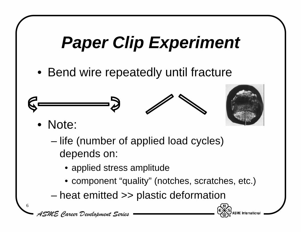
Paper Clip Experiment

• Bend wire repeatedly until fracture

• Note:– life (number of applied load cycles)

depends on: • applied stress amplitude• component “quality” (notches, scratches, etc.)

– heat emitted >> plastic deformation

7

Characteristics of Fatigue

• “Brittle” fracture surface appearance • Cracks often form at free surface• Macro/micro “beach marks”/ “striations”

0.3 in

Beach marks

20 µ m

Striations

8

Fatigue is problem for many types of structures

9

Exercise

Describe fatigue failures from your personal experience– What was cause of fatigue failure?– What was nature of cyclic load?– Was initial quality an issue? – How was failure detected?– How was problem solved?

10

ExerciseEstimate the fatigue lifetime needed for:

– Automobile axle– Railroad rail– Commercial aircraft components

• landing gear• lower wing skin

– Highway drawbridge mechanism– Space shuttle solid propellant rocket motor

cases

11

Exercise• Give an example of a High Cycle

Fatigue (HCF) application. – What is the required lifetime?– What are consequences of failure?

• Given an example of a Low Cycle Fatigue (LCF) application.– What is the required lifetime?– What are consequences of failure?

12

Fatigue Crack Formation

13

Crack Formation

Fracture

Crack Growth

Elapsed Cycles N

Cra

ck L

engt

h (a

)

Fatigue Crack Formation

Objective– Characterize resistance to fatigue crack formation– Predict number of cycles to “initiate” small* fatigue crack

in component *crack size ~ 0.03 inch

= “committee” crack

Approach– Stress-life concepts

(S-N curves)– Strain-life concepts

14

Stress-life (S-N) ApproachConcept: Stress range controls fatigue life

S

S

Log cycles N

∆S/2

Note:• Life increases as load amplitude decreases• Considerable scatter in data• “Run-outs” suggest “infinite life” possible• Life N usually total cycles to failure

S

time

∆S

15

Model Stress-life (S-N) Curve

• Se = endurance limitfor steels– Se ~ 0.5 ultimate stress Sult

– Se ~ 100 ksi if Sult ⟨ 200 ksiLog reversals 2N

Log

∆S

/2

Se

∆S/2 = σf ’ (2N)b

• σf ’ = fatigue strength coefficient• b = fatigue strength exponent

typically -0.12 < b < -0.05

Note: Measure life in terms of reversals 2N(1 cycle = 2 reversals)

16

S-N Curve: Mean Stress

Mean stress effects lifestress ratio R = Smin / Smax

Smean = 0.5(Smin + Smax)Sa = 0.5(Smax - Smin) = ∆S/2

Mean stress models

Sa/Se + Sm/Sult = 1

∆S/2 = (σf ’ - Smean) (2N)b

Mean Stress

Str

ess

Am

plitu

de

N = 106

N = 103

“Haigh” constant life diagram

S

timeSmin

Smax

∆S = 2Sa

17

S-N Curve: Other Factors• S-N curves are very sensitive to

– surface finish, coatings, notches– prior loading, residual stresses– specimen size effects, etc.

• Many empirical “knock-down” factors• S-N approach best suited for HCF (High

Cycle Fatigue) applications– limited by local plastic deformation– strain-life approach better for LCF (Low

Cycle Fatigue)

18

Strain-life (ε - N) ApproachConcept: Strain range ∆ε controls lifeExperiment• Control ∆ε

• Measure– “Reversals” (2Nf)

to failure (1 cycle= 2 reversals)

– Stable stress range ∆σneeded to maintain ∆ε

Note: “stable” ∆σ usually occursby mid-life (2Nf /2)

∆σ

∆εtime

ε∆ε

∆σ

time

σ

19

Cyclic Stress-Strain CurveRelate stable cyclic stress and strain ranges

∆σ

time

σ

time

ε ∆ε

∆σ

∆ε

∆ε

σ

ε∆σ

“Hystersis” loop

∆ε/2

∆σ/2

∆ε/2 = ∆σ/2E + (∆σ/2K’)1/n’

Cyclic stress-strain curve

E = elastic modulusK’ = cyclic strength coefficientn’ = strain hardening exponent

20

Plastic Strain-Life Curve

Relate “plastic” strain amplitude ∆εp/2 with reversals to failure 2Nf

Compute ∆εp/2 = ∆ε/2 - ∆σ/2E = total - “elastic” strain amplitudes

Log

∆ε p/2

Log 2Nf

∆εp/2 = εf ’ (2Nf)c

εf ’ = fatigue ductility coefficient

c = fatigue ductility exponent

typically -0.7 < c < -0.5

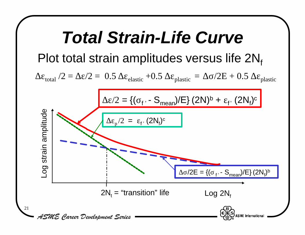
21

Total Strain-Life CurvePlot total strain amplitudes versus life 2Nf

∆εtotal /2 = ∆ε/2 = 0.5 ∆εelastic +0.5 ∆εplastic = ∆σ/2E + 0.5 ∆εplastic

∆ε/2 = {(σf ’ - Smean)/E} (2N)b + εf ’ (2Nf)c

∆εp /2 = εf ’ (2Nf)c

∆σ/2E = {(σ f ’ - Smean)/E} (2Nf)b

Log 2Nf

Log

stra

in a

mpl

itude

2Nt = “transition” life

22

Total Strain-Life

Note:– Plastic strain dominates for LCF– Elastic strain dominates for HCF– Transition life 2Nt separates LCF/HCF

∆εp =εf ’(2Nf)c

∆ε/2 = {(σf ’ - Smean )/E} (2N)b + εf ’ (2Nf)c

Log 2N f

Log

stra

in a

mpl

itude

∆σ/2E = {(σ f ’ - Smean)/E} (2Nf)b

2N t = “transition” life

LCFHCF

23

Variable Amplitude Loading

• Load amplitude varies in many applications

• Use of constant amplitude S - N or ε - N data requires “damage model”

• Miner’s rule*

Σ(Ni/Nf) = 1

Ni = number of applied cycles of stress amplitude SaiNf = fatigue life for Sai cycling only

*Use with caution!

S

time

Ni

2Sai

24

Example ProblemAssume:

– σf ’ = 220 ksi, b = - 0.1– stress history shown (1 block of loading)

Find: number of blocks to failure

+ 80 ksiS

time

- 80 ksi

- 100 ksi

+ 100 ksi

2N = 100

2N = 1000

2N = 1000S

S

25

Solution

Σ(Ni/Nf) = 1 2Nf = {(∆S/2) / (σf ’ - Smean)}1/b

Σ(Ni/Nf) = 1

When:1/0.0089 = 112.5

Answer112 blocks

∆S/2(ksi)

Smean

(ksi)2Nf 2Ni Ni/Nf

80 0 24,735 100 0.0040

50 +50 206,437 1000 0.0048

50 -50 21 E6 1000 4.74 E-6

0.0089

26

Load Sequence Effects• Hi-lo strain ε sequence

results in compressivemean stress σ when last large ε peak is tension

• → increases life• If last ε peak had been

compression, would result in tensile mean stress

• → decreases life

Load sequence important!

ε

σε

σt

t

Mean stress

27

Notch Fatigue• Notches can reduce life• Define Fatigue Notch Factor

Kf

Kf = Smooth/notch fatigue strength at 106 cycles

= ∆Ss /∆Sn

1 < Kf < Kt

(Kt = elastic stressconcentration factor)

Kf = 1 → no notch effectKf = Kt → full notch effect

Smooth

Notch

∆S/2

Log cycles N

∆Ss /2

∆Sn /2

106

28

Neuber’s RuleKf = fatigue notch concentration factor(∆s,∆e) = nominal stress/strain ranges

(away from notch)(∆σ,∆ε) = notch stress/strain rangesNeuber’s rule relates notch and

nominal stress/strain behavior

Solve with:

Kf2∆s∆e = ∆σ∆ε

∆ε/2 = ∆σ/2E + (∆σ/2K ’)1/n’

∆ε/2 = {(σf ‘ - Smean)}(2Nf)b + εf ‘(2Nf)c

(∆σ,∆ε)

(∆s,∆e)

29

Summary “Initiation” Methods• Total strain-life approach combines:

– original S-N curve (best suited for HCF) and– plastic strain-life method developed for LCF

problems

• S-N and strain-life often viewed as crack “initiation” approaches– actually deal with life to form “small” crack– crack size implicit in specimen/test procedure– typically assume “committee crack” ~ 0.03 in.

30

Initiation Summary Cont’

• Notches increase local stress/strain and often are source for crack formation– complex problem leads to local plasticity– characterize by fatigue notch concentration

factor Kf,, Neuber’s rule

• Load interaction effects result in local mean stress– can increase/decrease life– invalidate Miner’s rule

31

Fatigue Crack Growth

32

Crack Growth Approach

• Assumes entire lifefatigue crack growth – ignores “initiation” – assumes component

cracked before cycling begins

• Used with “damage tolerant design” – protects from pre-existent (or service) damage– based on linear elastic fracture mechanics

Elapsed Cycles N

Crack Growth

Cra

ck L

engt

h (a

)

Fracture

Initial crack

33

Damage Tolerance

The ability of a structure to resist priordamage for a specified period of time

Initial damage– material– manufacturing– service induced– size based on

inspection capability,experience, . . .

time

Cra

ck

size

Desired Life

34

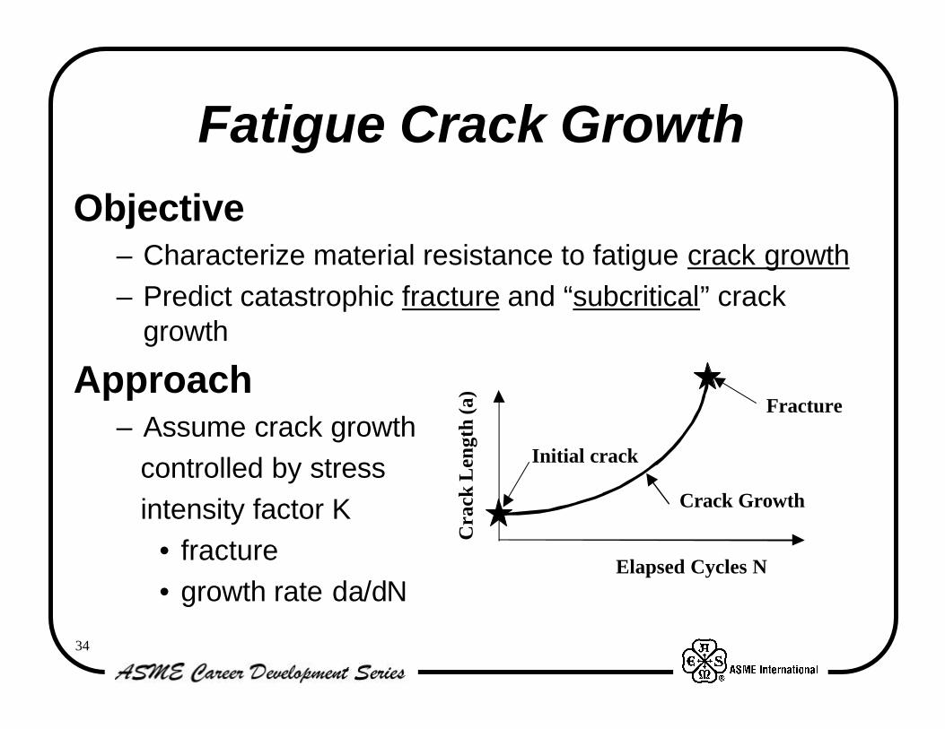
Fatigue Crack GrowthObjective

– Characterize material resistance to fatigue crack growth– Predict catastrophic fracture and “subcritical” crack

growth

Approach– Assume crack growth

controlled by stress intensity factor K

• fracture• growth rate da/dN

Elapsed Cycles N

Crack Growth

Cra

ck L

engt

h (a

)

Fracture

Initial crack

35

Stress Intensity Factor KI

KI is key linear elastic fracture mechanics parameter that relates:– applied stress: σ– crack length: a– component geometry: β(a)

(β(a) is dimensionless) a

Crack

σ

σ

β = 1.12

βπσ aK =I

Note units: stress-length1/2

36

Stress Intensity Factors

2a

W

σ

σ

K a Seca

W=

σ ππ

12

σ = Remote Stress

20 95

aW

≤ .

W

a

σ

σ

h

aW

≤ 0 6.

aW

β

hW

≥ 1 0.

K a

aW

aW

=

= −

+

σ π

β 112 0 231 10. 55. . aW

aW

aW

−

+

21 73 30 39

2 3 4

. .

For and

Many KIsolutions available

37

Crack tip Stress Fields

( )

+=→

=→

==

=

+=

−=

yxz

z

yzxz

Ixy

Iy

Ix

rKr

Kr

K

σσνσ

σ

σσ

θθθπ

σ

θθθπ

σ

θθθπ

σ

strain plane

0stress plane

02

3cos2

cos2

sin2

23

sin2

sin12

cos2

23

sin2

sin12

cos2

Theory of elasticity gives elastic stresses near crack tip in terms of stress intensity factor KI

All crack configurations have same singular stress field at tip(are similar results for other modes of loading, i.e., modes II and III)

Crack

x

y

θ

r

σxy

σy

σx

38

Kc Fracture Criterion

• Fracture occurs when K > constant = Kc

• Kc = material property = fracture toughness

• Criterion relates:– crack size: a– stress: σ– geometry: β(a)– material: Kc

• Plasticity limits small crack applications

σ

σ

2a

σult

Frac

ture

Stre

ss σ

Crack Size a

( )K a ac = σ π β

39

Fracture Toughness KcTypical Kc values (thick plate)

Note Kc depends on:– specimen thickness -- Kc decreases as

thickness increases until reaching minimum -KIc = plane strain toughness

– crack direction (material anisotropy)

Μaterial(thick plate)

2024−Τ351 Ti-6Al-4VΑluminum Αluminum Titanium

7075−Τ651 300M Steel 18 Nickel

Κc 31 26 112 47 100

(235 ksi yield) (200 ksi yield)

(ksi in1/2)

40

Fracture Example

Member A fractures when crack length a = 2.0 inch and remote stress = 5 ksi

What stress will fracture member B (assume same material)?

2.0 in

4.0 in

5 ksi

5 ksi

A

5 in

8 in

σ = ?

σ = ?

B

41

Fracture Example SolutionEdge crack

K = σ(πa)1/2 β(a) = Kc at fracture

a/w = 2/4 σ = 5 a = 2 → β = 2.83Kc = 35.5 ksi-in1/2 = constant

Center CrackK = σ (π a)1/2β(a) β(a) = [Sec (π a/W)]1/2

a = 2.5 W = 8 → β = 1.34K = Kc at fracture = 35.5

2.0 in

4.0 in

5 ksi

5 ksi

5 in

8 in

σ = ?

σ = ?

a

W

a

W

= −

+β 1 12 0 231 10. 55. .

a

W

a

W

a

W

−

+

21 73 30 39

2 3 4

. .

→ σf = 9.5 ksi

42

Fatigue Crack GrowthGoal: show cyclic stress intensity factor ∆K

controls crack growth rate da/dN

∆P = constant

time

P

2a

∆P

Crack Face Load

2a

∆σ

Remote Load

∆σ = constant

time

σ

Same material

Different loadings

43

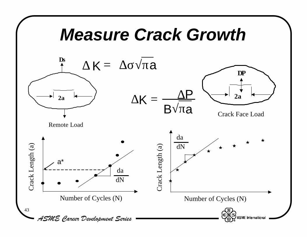
Measure Crack Growth

2a

∆σ

Remote Load

2a

∆P

Crack Face Load

dadN

Cra

ck L

engt

h (a

)

Number of Cycles (N)

=∆K ∆PB√πa

∆ K = ∆σ√πa

Cra

ck L

engt

h (a

)

Number of Cycles (N)

dadN

a*

44

Correlate Rate da/dN vs ∆KC

rack

Len

gth

(a)

Number of Cycles (N)

dadN

2a

2a

Cra

ck L

engt

h (a

)

Number of Cycles (N)

dadN

a*

∆KthKc

Log ∆ K

Log

da/d

N

∆ ∆K a= σ π

∆∆

KP

B a=

π

45

da/dN Vs ∆K

∆Kth

Kc

Log ∆K

Log

da/d

N

Note: • ∆K correlates fatigue

crack growth rate da/dN• ∆K accounts for crack

geometry• No crack growth for

da/dN < ∆Kth

• Fractures when Kmaxin the ∆K range à Kc

• da/dN - ∆K curve is material property

46

Sample Crack Growth Data• da/dN - ∆K data for

7075-T6 aluminum• Note effect of stress

ratio R = min/max stress (da/dN ↑as R↑)

• Reference: Military Handbook-5

• Other handbook data are available

47

Model da/dN - ∆K CurveFit test data with numerical models such as:

∆Kth

Kc

Log ∆K

Log

da/d

N

dadN

F K= ( ) dadN

C K m= ∆

dadN

C KR K K

m

c

=− −

∆∆( )1

Here C, m, Kc are empirical constants

R = min/max stress(are many other models)

Paris

Forman

48

Compute Fatigue Life Nf

ao, af = initial, final crack sizesF(K) = function of:

– cyclic stress: ∆σ, R, . . .– crack geometry: β(a)– crack length: a– material

Nda

F Kf a

a

o

f= ∫ ( )

dadN

F K= ( )

∆σ

time

σ

2a

∆σ

49

Example Life Calculation

a

Crack

σ

σ

∆σ = constant

time

σ

Given: edge crack in wide plateKc= 63 ksi-in1/2

initial crack ai = 0.5 inchcyclic stress ∆σ = 10 ksi, R = 0

(∆σ = σmax = 10 ksi)

da/dN = 10-9∆K4

Find: a) cyclic life Nfb) life if initial crack size

decreased to ai = 0.1 inchNote: at fracture K = Kc = 63 = 1.12σmax (πa)1/2

→ final crack af = 10 inch

50

Solution

[ ] = = ∫∫

daC K

da

C am ma

a

a

a

o

f

o

f

∆ ∆112. σ πNf

( ) ( )[ ]N

C ma af m f

mo

m=−

−− −1

112 1 5

1 5 1 5

. .

. .

∆σ π

K a= σ π 112.dadN

C K m= ∆

a) Nf = 12,234 cycles (ai = 0.5)b) Nf = 63,747 cycles (ai = 0.1)Note: big influence of initial crack length!

51

Fatigue Crack Retardation

Time

App

lied

Stre

ss (

σ)

Overload

Without Overload

With Overload

“Retardation”

Cra

ck L

engt

h (a

)

Elapsed Cycle (N)

Note “load interaction effect”• Tensile overload can “retard” crack growth (increase life)• Life increase due to crack tip plasticity• Depends on magnitude/sequence of overload, material, …• Are empirical retardation models

52

Cycle-by-Cycle Calculation

Compute cycle-by-cycle growth in crack length a– acurrent = aprior + da/dNcurrent

– da/dNcurrent = F(Kcurrent) * “Retardation” term– Sum for all cycles in spectrum

Powerful technique for computer programming

σn

σn+1

App

lied

Stre

ss (σ

)

Time (t)

Variable amplitude loading prevents simple life integration

53

Crack Growth Summary• Fracture mechanics approach assumes

entire fatigue life is crack growth• Stress intensity factor K controls fracture

and growth rate da/dN– K = σ[πa]1/2 β(a)– Fracture: K = Kc

– Fatigue: da/dN = F(∆K)– Integrate da/dN for life

• Are load interaction and other effects (see references)

54

Fatigue Design/Repair Concepts

55

Design Philosophies

Fatigue Design Criteria• Infinite Life• Safe-Life• Damage Tolerant

– Fail-safe– Slow crack growth

• Retirement-for-cause

a

σ

Crack

σ

Str

ess

Time

Crack Formation

Fracture

Crack Growth

Elapsed Cycles N

Pre-CrackCra

ck L

engt

h (a

)

56

Infinite Life Criterion

Design Goal: prevent fatigue damage from everdeveloping (i.e. infinite life)

• Usually based on endurance limit • Could also employ threshold K concepts• Leads to small design stresses/heavy members• Limited to simple components/loading• Often impractical/not achievable in practice

– Weight critical structure– Complex loads

57

Safe-Life CriterionDesign goal: component is to remain crack free for

finite service life• Assumes initial crack-free structure• Establish “mean life” by test/analysis• Safety factors account for “scatter”

predicted mean

Desired life = mean/S.F.

Design Life

Failu

re

Oc

cu

rre

nc

e

1 32 4

Problems:• large safety factor• no protection from

initial damage

58

Fail-Safe CriterionDesign goal: contain single component failure

without losing entire structure• Assumes crack is present• Provide alternate load paths, redundant structure, crack

stoppers, etc.• Requires detection of 1st failure

Time

Cra

ck

size

1st member

2nd memberCrack arrest

59

Slow Crack Growth CriterionDesign goal: prevent initial crack from growing to

fracture during life of structure• Pre-existent crack size specified by inspection

limits, experience• Crack growth life

> service life x S.F.• Based on fatigue

crack growthresistance

• Emphasizes nondestructive inspection

Cra

ck

size

Desired Life

time

Fracture

60

Retirement-for-Cause

Failure size

Cra

ck L

engt

h

Time

inspect/repair

Design goal: Use periodic inspection/repairto achieve desired fatigue lives

Limited by repeated maintenance economics

61

Life Extension Concepts

Shot peenHole coldwork

Interference fastenersOverstress, etc.

Introduce BeneficialResidual Stresses

MetalComposite

Mechanical FastenBond

Doublers

HCF damping materials

Reduce Stressvia Reinforcement

Weight limitsFlight restrictions

etc.

Reduce OperatingLoads

No Cracks Found(assume small cracks)

MetalComposite Mechanical Fasten

Bond

Patches

Replace componentStop drill cracks

Welding

Repair CrackedStructure

Cracks Found

ComponentInspection

62

Summary• Fatigue is complex problem that

involves many disciplines• Fatigue affects design and operation of

many types of structures• Fatigue may be treated by several

methods/philosophies– Assume component cracked– Assume component uncracked– Probabilistic methods

63

64

Your Path to Lifelong Learning

ASME offers you exciting, rewarding ways to sharpen your technical skills, enhance personal development and prepare for advancement.

Short Courses – More than 200 short courses offered each you keep you up to speed in the technology fast lane—or, help you fill in any gaps in your technical background.

Customized Training at your organization’s site – Do you have ten or more people at your site who could benefit from an ASME course? Most of our courses can be offered in-house and tailored to your latest engineering project. Bring course to your company too.

Self-study materials meet the needs of individuals who demand substantive, practical information, yet require flexibility, quality and convenience. Return to each program again and again, as a refresher or as an invaluable addition to your reference library.

FE Exam Review– A panel of seasoned educators outline a wide range of required topics to provide a thorough review to help practicing engineers as well as engineering students prepare for this challenging examination. Videotape Review

PE Exam Review– A comprehensive review of all the major exam topics that demons trates the necessary math, logic and theory. Videotape, Online, or Online Live Review available.

65

FOR MORE INFORMATION CALL 1-800-THE-ASME

__________________________________________________________________________

INFORMATION REQUEST FORM

Please mail to ASME at 22 Law Drive, P. O. Box 2900, Fairfield, NJ 07007-2900, or fax to 973-882-1717, call 1-800-THE-ASME, or email infocentral@asme.org.

Send me information on the following:

____ Short Courses ____ In-House Training ____ Self-Study Programs

____ FE Exam Review ____ PE Exam Review (videotape) ____ PE Exam Review (Online)

____ PE Exam Review (Online Live)

Name: ______________________________________________

Title: _______________________________________________

Organization: _________________________________________

Business Address: _____________________________________

City: _________________ State: __ Zip Code: _____________

Business Phone: _________________ Fax: ________________

Email: ______________________________________________