Embed Size (px)
Citation preview
9a. Neural Networks
New lecture
Didn’t change the canonical numbering yet

2
9.1 Motivation
3
Biological Neural Nets
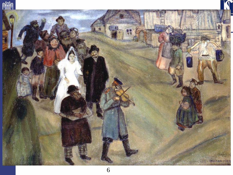
• Pigeons as art experts (Watanabe et al. 1995)
• Experiment:
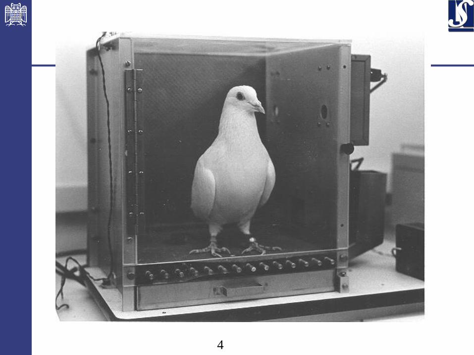
• Pigeon in Skinner box
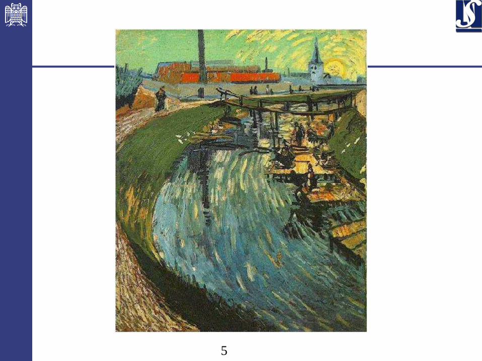
• Present paintings of two different artists (e.g.
Chagall / Van Gogh)
• Reward for pecking when presented a particular
artist (e.g. Van Gogh)
This section is based on slides by Torsten Reil
4
5
6
7
• Pigeons were able to discriminate between Van Gogh and
Chagall with 95% accuracy (when presented with pictures they
had been trained on)
• Discrimination still 85% successful for previously unseen
paintings of the artists
• Pigeons do not simply memorise the pictures
• They can extract and recognise patterns (the ‘style’)
• They generalise from the already seen to make predictions
• This is what neural networks (biological and artificial) are good at
(unlike conventional computer)
8
9.2 Feed-forward Network Functions
also know as multilayer perceptrons (MLP)
See Bishop “Pattern Recognition and Machine
Learning” sections 5.1 and 5.2
9
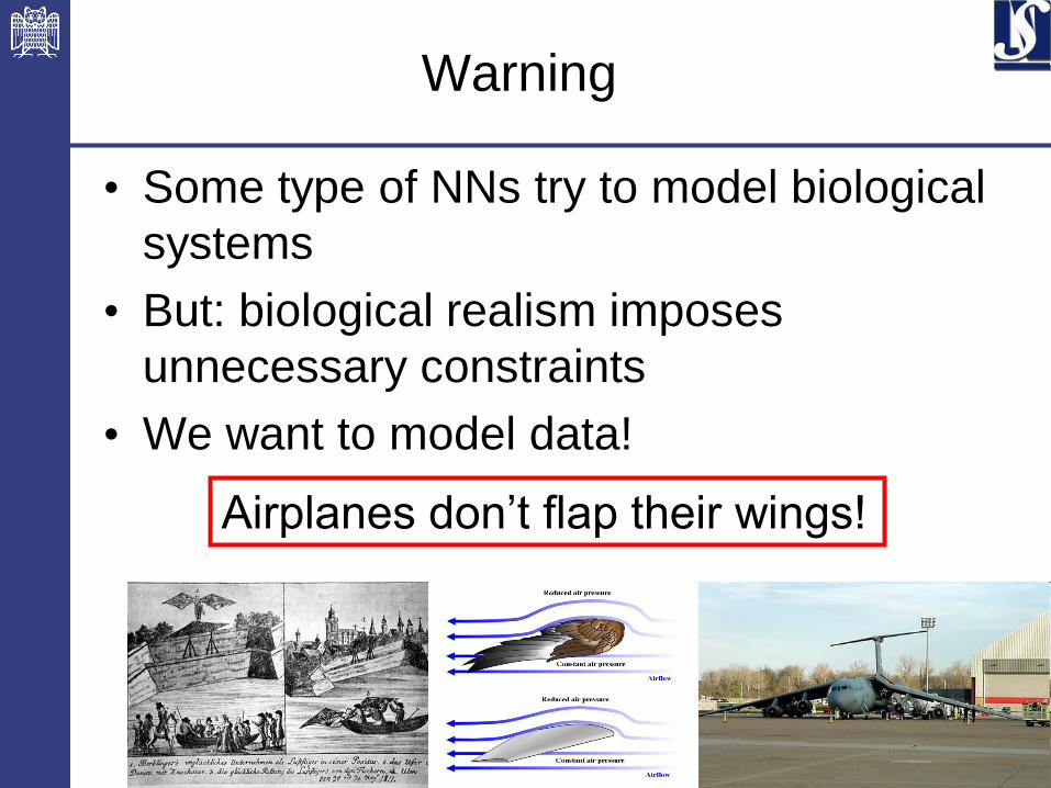
Warning
• Some type of NNs try to model biological
systems
• But: biological realism imposes
unnecessary constraints
• We want to model data!
Airplanes don’t flap their wings!
10
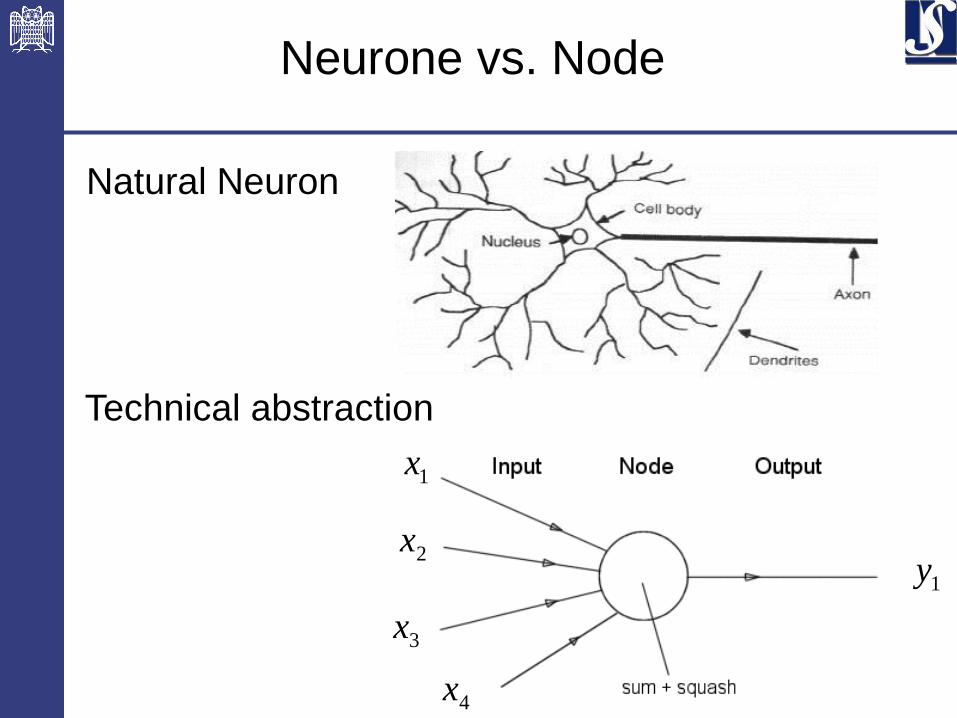
Neurone vs. Node
1x
2x
3x
4x
1y
Natural Neuron
Technical abstraction
11
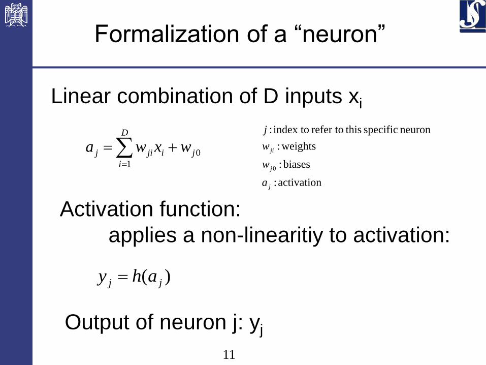
Formalization of a “neuron”
D
i
jijij wxwa1
0
)( jj ahy
Linear combination of D inputs xi
activation :
biases :
weights:
neuron specific thisrefer to index to :
0
j
j
ji
a
w
w
j
Activation function:
applies a non-linearitiy to activation:
Output of neuron j: yj

12
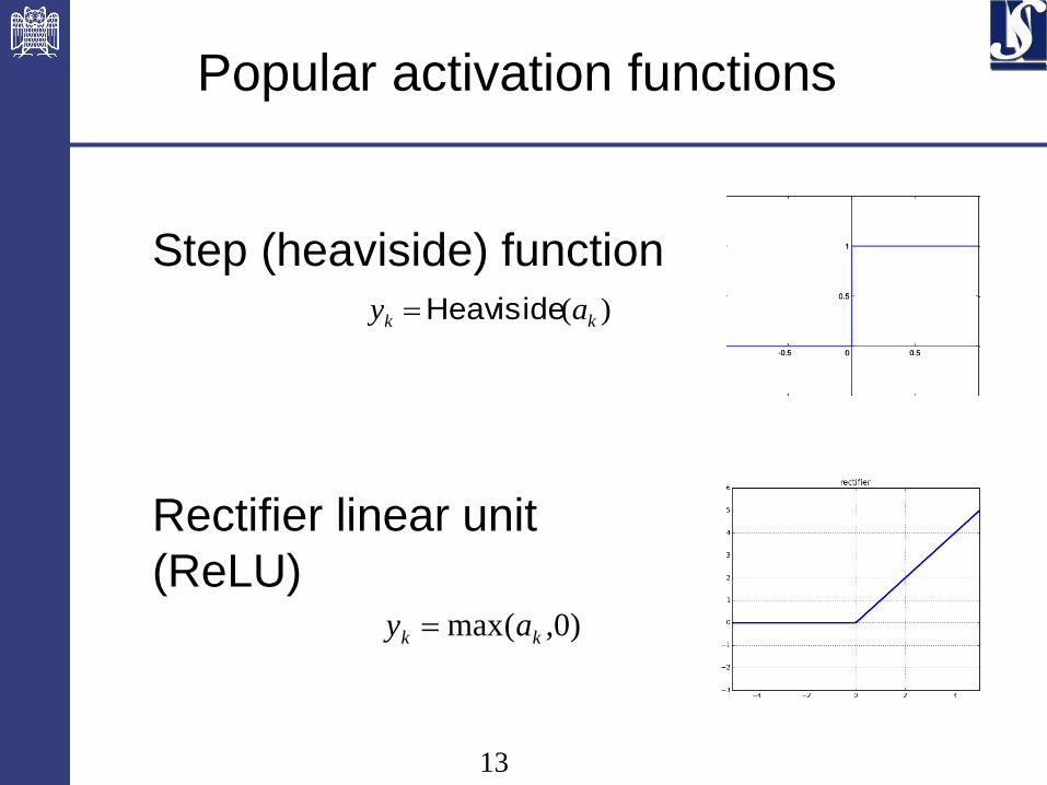
Popular activation functions
)tanh( kk ay
)exp(1
1
k
ka
y
“tanh”-function
Logistic sigmoid function
13
Popular activation functions
Step (heaviside) function )( kk ay Heaviside
Rectifier linear unit
(ReLU) )0,(max kk ay
14
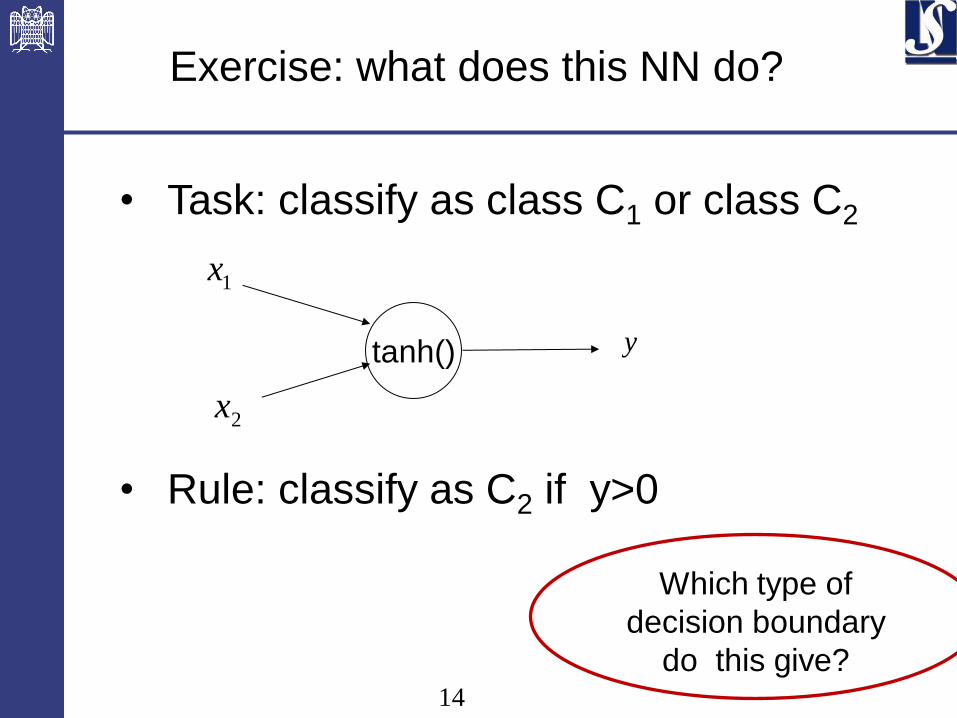
Exercise: what does this NN do?
tanh()
1x
2x
y
• Task: classify as class C1 or class C2
• Rule: classify as C2 if y>0
Which type of
decision boundary
do this give?
15
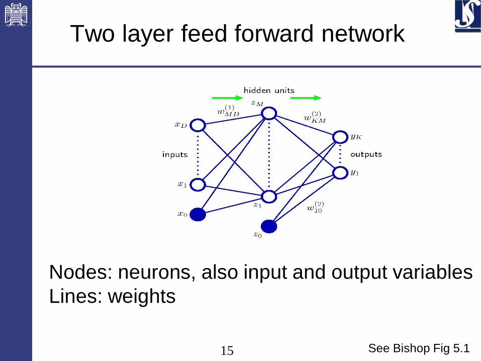
Two layer feed forward network
See Bishop Fig 5.1
Nodes: neurons, also input and output variables
Lines: weights
16
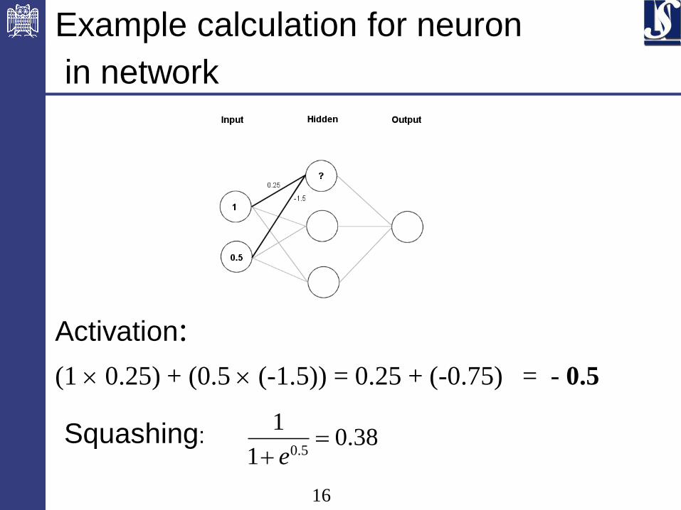
Example calculation for neuron
in network
Activation:
(1 0.25) + (0.5 (-1.5)) = 0.25 + (-0.75) = - 0.5
0.381
15.0
e
Squashing:
17
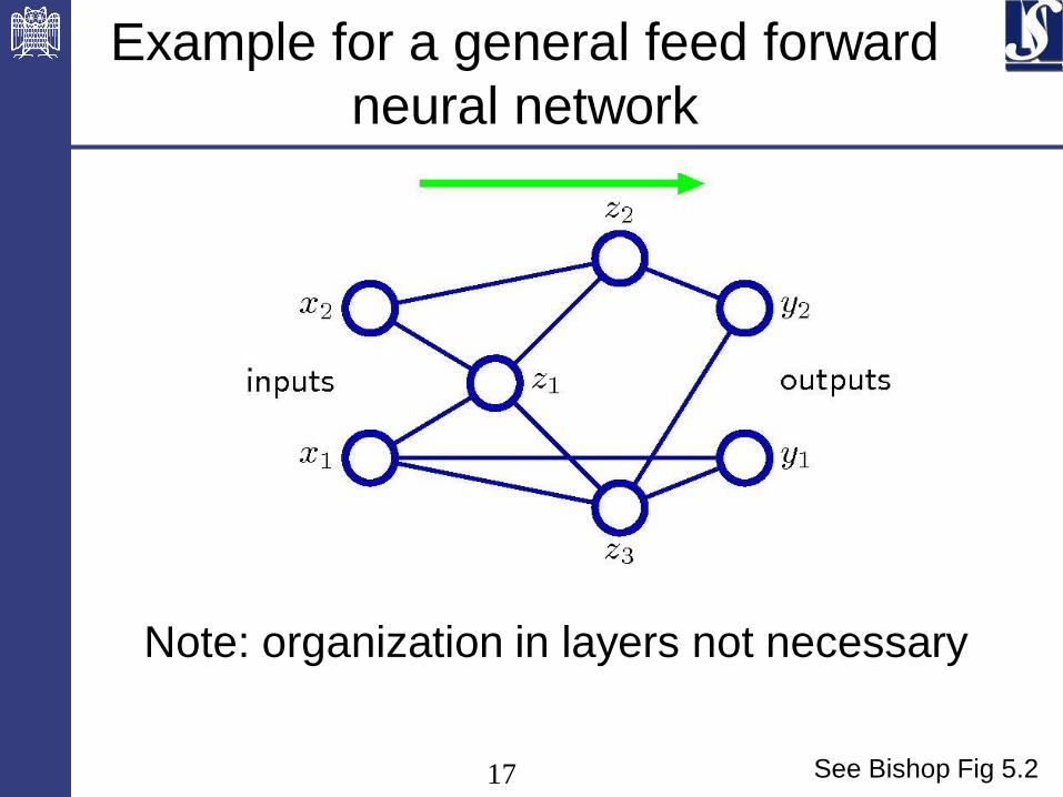
Example for a general feed forward
neural network
See Bishop Fig 5.2
Note: organization in layers not necessary
18
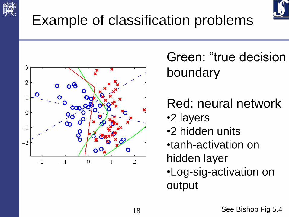
Example of classification problems
Green: “true decision
boundary
Red: neural network •2 layers
•2 hidden units
•tanh-activation on
hidden layer
•Log-sig-activation on
output
See Bishop Fig 5.4
19
• Neural Networks with at least one hidden layer are universal approximators
• They can approximate any function within some bound e
• For practical purposes of no use
Expressive Power of
multi-layer Networks
20
9.3 Network Training
21
Let
tn be the n-th target (or desired) output and
y(xn,w) be the n-th computed output with
n = 1, …, N and
Goal:
Find numerical values for weights wi,j
Goal of Network training
22
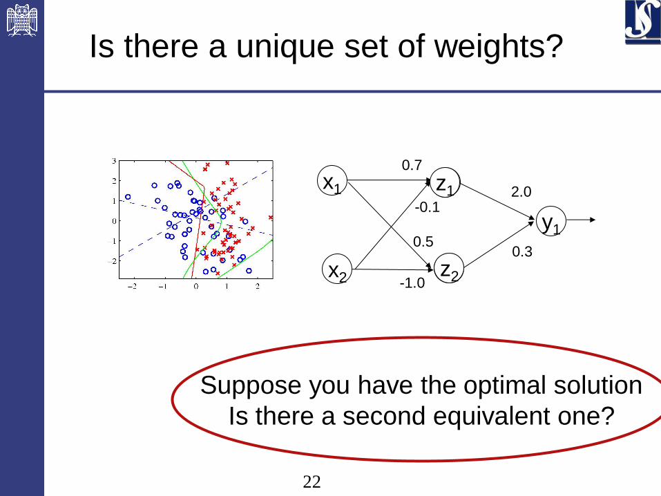
Is there a unique set of weights?
x1
x2
y1
Suppose you have the optimal solution
Is there a second equivalent one?
0.7
-0.1
0.5 0.3
2.0
-1.0
z1
z2
23
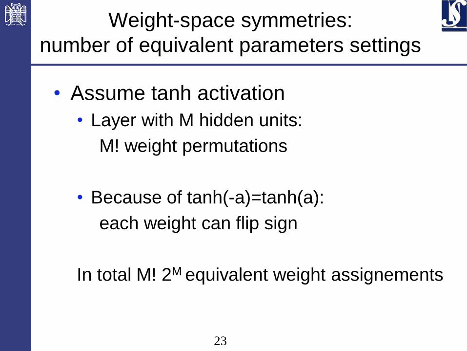
Weight-space symmetries:
number of equivalent parameters settings
• Assume tanh activation
• Layer with M hidden units:
M! weight permutations
• Because of tanh(-a)=tanh(a):
each weight can flip sign
In total M! 2M equivalent weight assignements
24
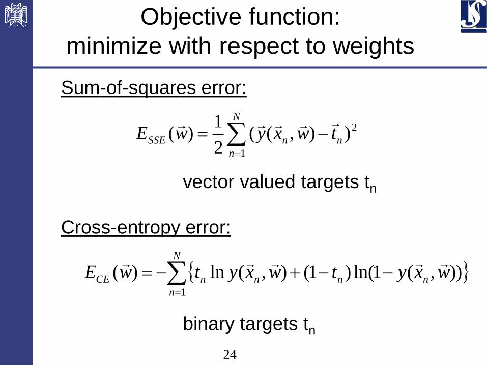
Sum-of-squares error:
vector valued targets tn
Cross-entropy error:
binary targets tn
N
n
nnSSE twxywE1
2)),((2
1)(
Objective function:
minimize with respect to weights
N
n
nnnnCE wxytwxytwE1
)),(1ln()1(),(ln)(
25
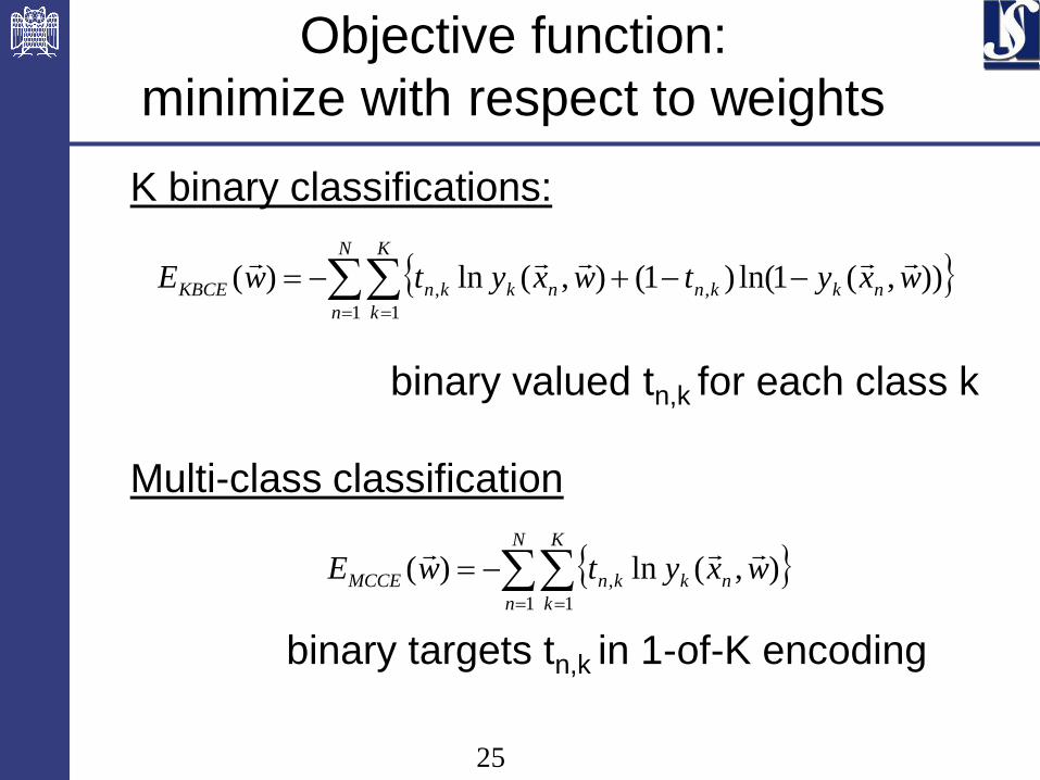
K binary classifications:
binary valued tn,k for each class k
Multi-class classification
binary targets tn,k in 1-of-K encoding
Objective function:
minimize with respect to weights
N
n
K
k
nkknnkknKBCE wxytwxytwE1 1
,, )),(1ln()1(),(ln)(
N
n
K
k
nkknMCCE wxytwE1 1
, ),(ln)(
26
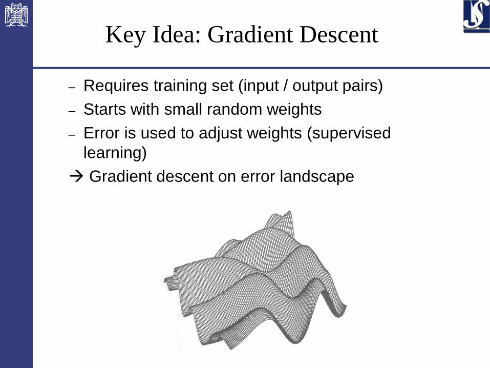
Key Idea: Gradient Descent
– Requires training set (input / output pairs)
– Starts with small random weights
– Error is used to adjust weights (supervised
learning)
Gradient descent on error landscape
27
Gradient Descent
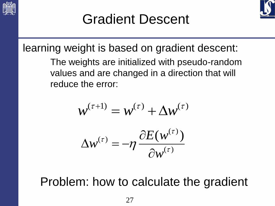
learning weight is based on gradient descent:
The weights are initialized with pseudo-random
values and are changed in a direction that will
reduce the error:
)(
)()( )(
w
wEw
)()()1( www
Problem: how to calculate the gradient
28
Calculating the Gradient 1:
Finite Differences
)()()()(
ee
eO
wEwE
w
wE jiji
ji
ji
)(2
)()()(2e
e
eeO
wEwE
w
wE jiji
ji
ji
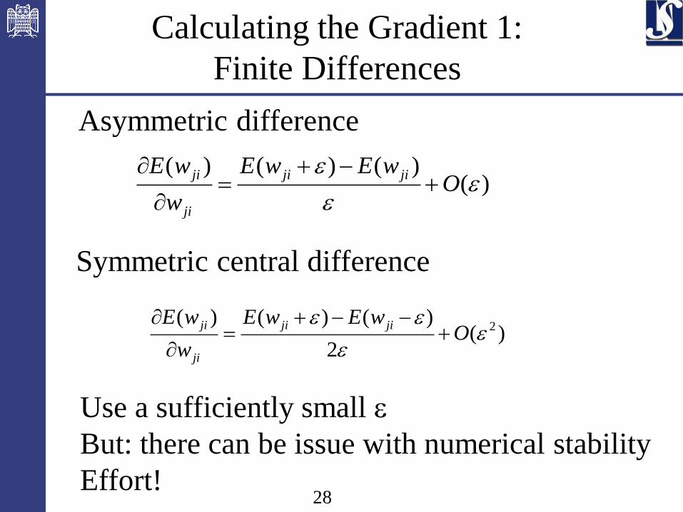
Asymmetric difference
Symmetric central difference
Use a sufficiently small e
But: there can be issue with numerical stability
Effort!

29
Back Propagation
See blackboard
30
Back Propagation
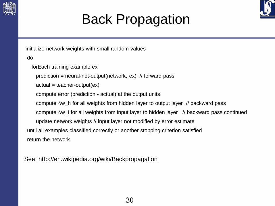
initialize network weights with small random values
do
forEach training example ex
prediction = neural-net-output(network, ex) // forward pass
actual = teacher-output(ex)
compute error (prediction - actual) at the output units
compute w_h for all weights from hidden layer to output layer // backward pass
compute w_i for all weights from input layer to hidden layer // backward pass continued
update network weights // input layer not modified by error estimate
until all examples classified correctly or another stopping criterion satisfied
return the network
See: http://en.wikipedia.org/wiki/Backpropagation
31
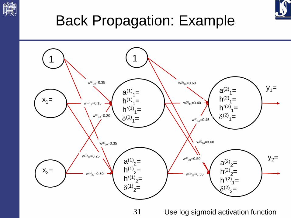
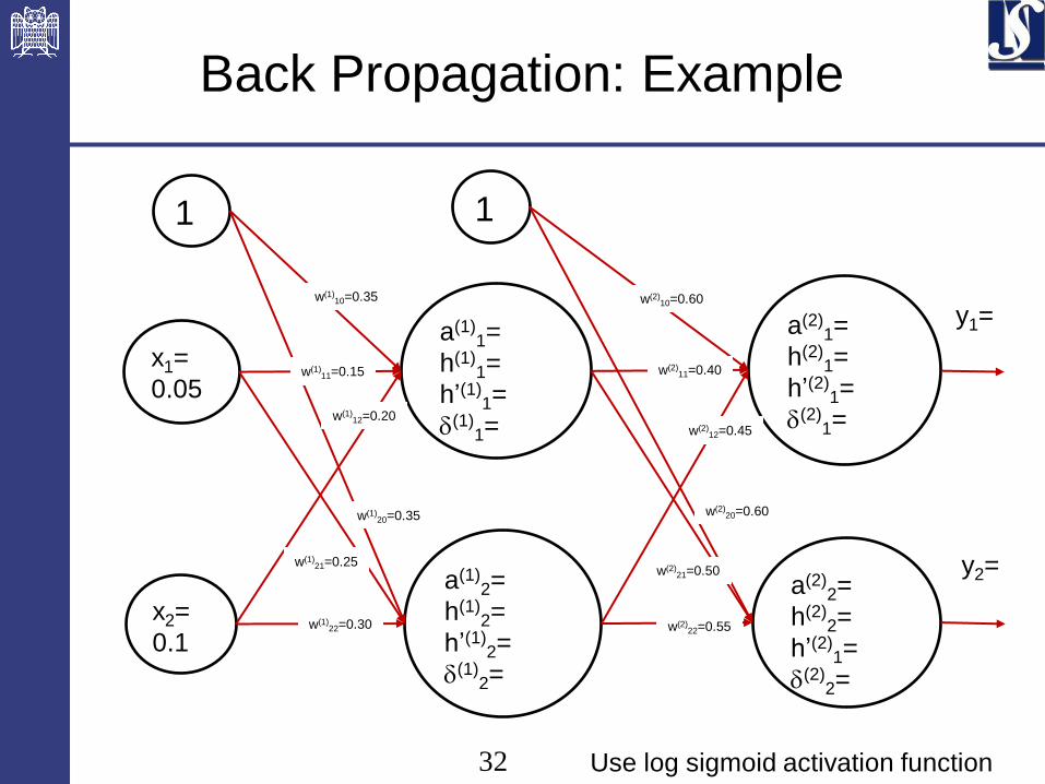
Back Propagation: Example
a(1)1=
h(1)1=
h’(1)1=
d(1)1=
a(1)2=
h(1)2=
h’(1)2=
d(1)2=
a(2)1=
h(2)1=
h’(2)1=
d(2)1=
a(2)2=
h(2)2=
h’(2)1=
d(2)2=
x1=
x2=
1 1
w(1)11=0.15
w(1)12=0.20
w(1)10=0.35
w(1)21=0.25
w(1)22=0.30
w(1)20=0.35
w(2)11=0.40
w(2)12=0.45
w(2)10=0.60
w(2)21=0.50
w(2)22=0.55
w(2)20=0.60
y1=
y2=
Use log sigmoid activation function
32
Back Propagation: Example
a(1)1=
h(1)1=
h’(1)1=
d(1)1=
a(1)2=
h(1)2=
h’(1)2=
d(1)2=
a(2)1=
h(2)1=
h’(2)1=
d(2)1=
a(2)2=
h(2)2=
h’(2)1=
d(2)2=
x1=
0.05
x2=
0.1
1 1
w(1)11=0.15
w(1)12=0.20
w(1)10=0.35
w(1)21=0.25
w(1)22=0.30
w(1)20=0.35
w(2)11=0.40
w(2)12=0.45
w(2)10=0.60
w(2)21=0.50
w(2)22=0.55
w(2)20=0.60
y1=
y2=
Use log sigmoid activation function

33
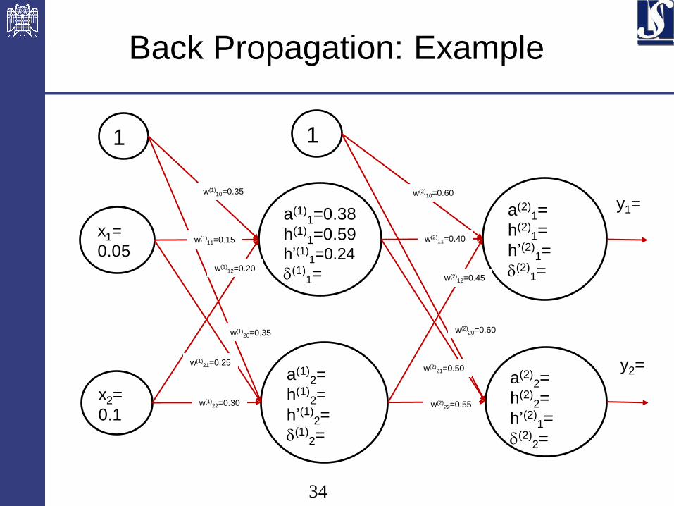
Back Propagation: Example
a(1)1=0.38
h(1)1=
h’(1)1=
d(1)1=
a(1)2=
h(1)2=
h’(1)2=
d(1)2=
a(2)1=
h(2)1=
h’(2)1=
d(2)1=
a(2)2=
h(2)2=
h’(2)1=
d(2)2=
x1=
0.05
x2=
0.1
1 1
w(1)11=0.15
w(1)12=0.20
w(1)10=0.35
w(1)21=0.25
w(1)22=0.30
w(1)20=0.35
w(2)11=0.40
w(2)12=0.45
w(2)10=0.60
w(2)21=0.50
w(2)22=0.55
w(2)20=0.60
y1=
y2=
34
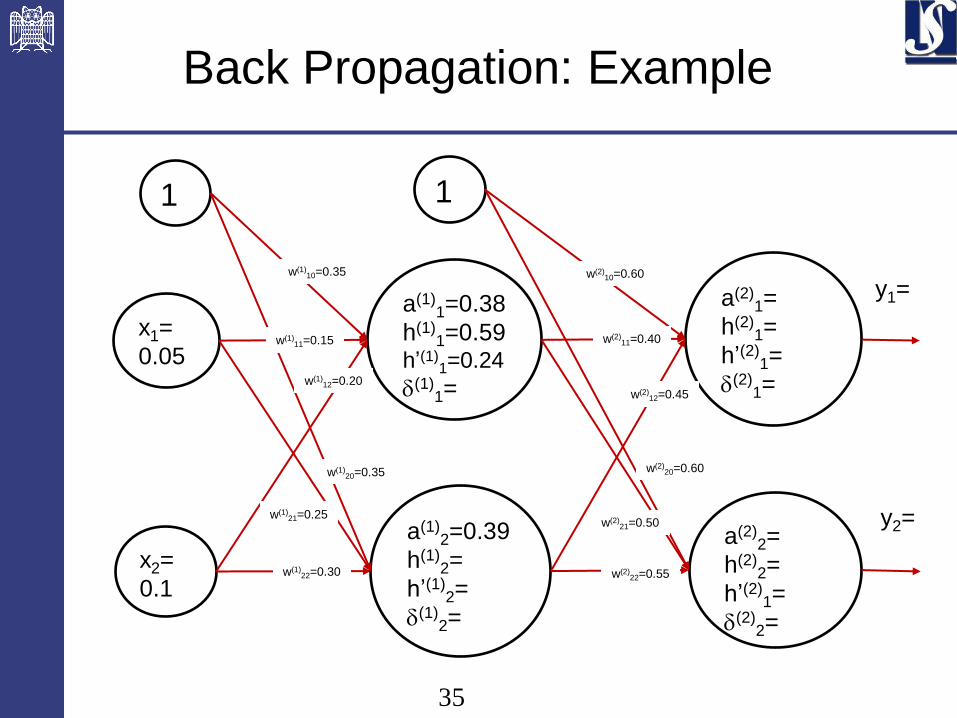
Back Propagation: Example
a(1)1=0.38
h(1)1=0.59
h’(1)1=0.24
d(1)1=
a(1)2=
h(1)2=
h’(1)2=
d(1)2=
a(2)1=
h(2)1=
h’(2)1=
d(2)1=
a(2)2=
h(2)2=
h’(2)1=
d(2)2=
x1=
0.05
x2=
0.1
1 1
w(1)11=0.15
w(1)12=0.20
w(1)10=0.35
w(1)21=0.25
w(1)22=0.30
w(1)20=0.35
w(2)11=0.40
w(2)12=0.45
w(2)10=0.60
w(2)21=0.50
w(2)22=0.55
w(2)20=0.60
y1=
y2=
35
Back Propagation: Example
a(1)1=0.38
h(1)1=0.59
h’(1)1=0.24
d(1)1=
a(1)2=0.39
h(1)2=
h’(1)2=
d(1)2=
a(2)1=
h(2)1=
h’(2)1=
d(2)1=
a(2)2=
h(2)2=
h’(2)1=
d(2)2=
x1=
0.05
x2=
0.1
1 1
w(1)11=0.15
w(1)12=0.20
w(1)10=0.35
w(1)21=0.25
w(1)22=0.30
w(1)20=0.35
w(2)11=0.40
w(2)12=0.45
w(2)10=0.60
w(2)21=0.50
w(2)22=0.55
w(2)20=0.60
y1=
y2=
36
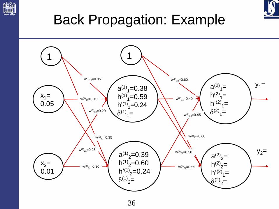
Back Propagation: Example
a(1)1=0.38
h(1)1=0.59
h’(1)1=0.24
d(1)1=
a(1)2=0.39
h(1)2=0.60
h’(1)2=0.24
d(1)2=
a(2)1=
h(2)1=
h’(2)1=
d(2)1=
a(2)2=
h(2)2=
h’(2)1=
d(2)2=
x1=
0.05
x2=
0.01
1 1
w(1)11=0.15
w(1)12=0.20
w(1)10=0.35
w(1)21=0.25
w(1)22=0.30
w(1)20=0.35
w(2)11=0.40
w(2)12=0.45
w(2)10=0.60
w(2)21=0.50
w(2)22=0.55
w(2)20=0.60
y1=
y2=
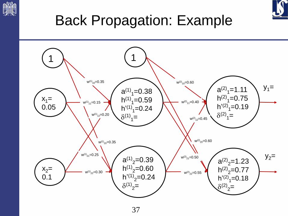
37
Back Propagation: Example
a(1)1=0.38
h(1)1=0.59
h’(1)1=0.24
d(1)1=
a(1)2=0.39
h(1)2=0.60
h’(1)2=0.24
d(1)2=
a(2)1=1.11
h(2)1=0.75
h’(2)1=0.19
d(2)1=
a(2)2=1.23
h(2)2=0.77
h’(2)1=0.18
d(2)2=
x1=
0.05
x2=
0.1
1 1
w(1)11=0.15
w(1)12=0.20
w(1)10=0.35
w(1)21=0.25
w(1)22=0.30
w(1)20=0.35
w(2)11=0.40
w(2)12=0.45
w(2)10=0.60
w(2)21=0.50
w(2)22=0.55
w(2)20=0.60
y1=
y2=
38
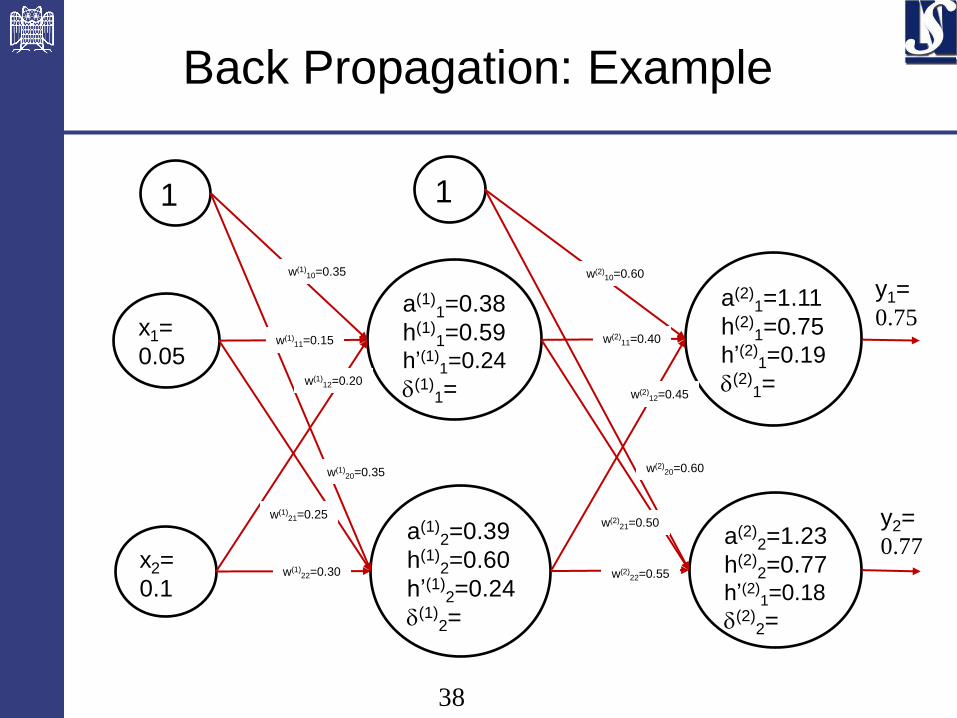
Back Propagation: Example
a(1)1=0.38
h(1)1=0.59
h’(1)1=0.24
d(1)1=
a(1)2=0.39
h(1)2=0.60
h’(1)2=0.24
d(1)2=
a(2)1=1.11
h(2)1=0.75
h’(2)1=0.19
d(2)1=
a(2)2=1.23
h(2)2=0.77
h’(2)1=0.18
d(2)2=
x1=
0.05
x2=
0.1
1 1
w(1)11=0.15
w(1)12=0.20
w(1)10=0.35
w(1)21=0.25
w(1)22=0.30
w(1)20=0.35
w(2)11=0.40
w(2)12=0.45
w(2)10=0.60
w(2)21=0.50
w(2)22=0.55
w(2)20=0.60
y1=
0.75
y2=
0.77
39
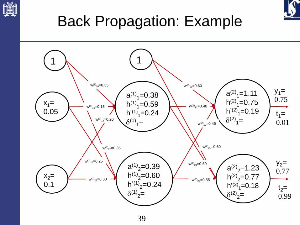
Back Propagation: Example
a(1)1=0.38
h(1)1=0.59
h’(1)1=0.24
d(1)1=
a(1)2=0.39
h(1)2=0.60
h’(1)2=0.24
d(1)2=
a(2)1=1.11
h(2)1=0.75
h’(2)1=0.19
d(2)1=
a(2)2=1.23
h(2)2=0.77
h’(2)1=0.18
d(2)2=
x1=
0.05
x2=
0.1
1 1
w(1)11=0.15
w(1)12=0.20
w(1)10=0.35
w(1)21=0.25
w(1)22=0.30
w(1)20=0.35
w(2)11=0.40
w(2)12=0.45
w(2)10=0.60
w(2)21=0.50
w(2)22=0.55
w(2)20=0.60
y1=
0.75
y2=
0.77
t1=
0.01
t2=
0.99
40
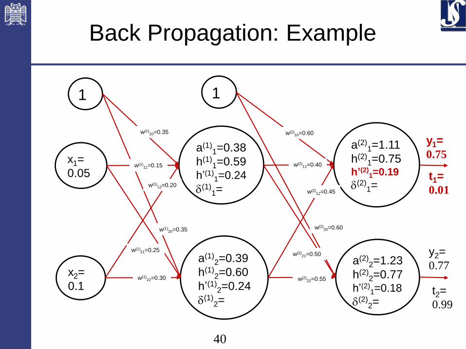
Back Propagation: Example
a(1)1=0.38
h(1)1=0.59
h’(1)1=0.24
d(1)1=
a(1)2=0.39
h(1)2=0.60
h’(1)2=0.24
d(1)2=
a(2)1=1.11
h(2)1=0.75
h’(2)1=0.19
d(2)1=
a(2)2=1.23
h(2)2=0.77
h’(2)1=0.18
d(2)2=
x1=
0.05
x2=
0.1
1 1
w(1)11=0.15
w(1)12=0.20
w(1)10=0.35
w(1)21=0.25
w(1)22=0.30
w(1)20=0.35
w(2)11=0.40
w(2)12=0.45
w(2)10=0.60
w(2)21=0.50
w(2)22=0.55
w(2)20=0.60
y1=
0.75
y2=
0.77
t1=
0.01
t2=
0.99
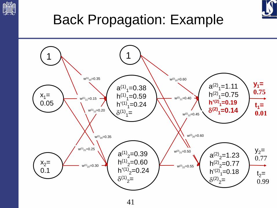
41
Back Propagation: Example
a(1)1=0.38
h(1)1=0.59
h’(1)1=0.24
d(1)1=
a(1)2=0.39
h(1)2=0.60
h’(1)2=0.24
d(1)2=
a(2)1=1.11
h(2)1=0.75
h’(2)1=0.19
d(2)1=0.14
a(2)2=1.23
h(2)2=0.77
h’(2)1=0.18
d(2)2=
x1=
0.05
x2=
0.1
1 1
w(1)11=0.15
w(1)12=0.20
w(1)10=0.35
w(1)21=0.25
w(1)22=0.30
w(1)20=0.35
w(2)11=0.40
w(2)12=0.45
w(2)10=0.60
w(2)21=0.50
w(2)22=0.55
w(2)20=0.60
y1=
0.75
y2=
0.77
t1=
0.01
t2=
0.99

42
Back Propagation: Example
a(1)1=0.38
h(1)1=0.59
h’(1)1=0.24
d(1)1=
a(1)2=0.39
h(1)2=0.60
h’(1)2=0.24
d(1)2=
a(2)1=1.11
h(2)1=0.75
h’(2)1=0.19
d(2)1=0.14
a(2)2=1.23
h(2)2=0.77
h’(2)1=0.18
d(2)2=
x1=
0.05
x2=
0.1
1 1
w(1)11=0.15
w(1)12=0.20
w(1)10=0.35
w(1)21=0.25
w(1)22=0.30
w(1)20=0.35
w(2)11=0.40
w(2)12=0.45
w(2)10=0.60
w(2)21=0.50
w(2)22=0.55
w(2)20=0.60
y1=
0.75
y2=
0.77
t1=
0.01
t2=
0.99
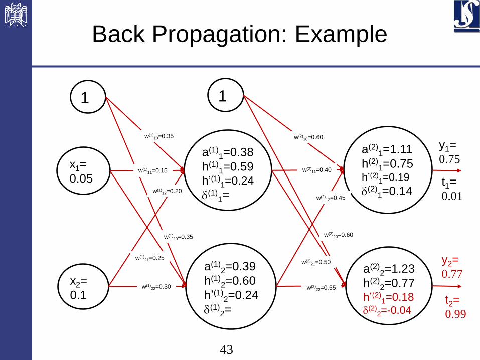
43
Back Propagation: Example
a(1)1=0.38
h(1)1=0.59
h’(1)1=0.24
d(1)1=
a(1)2=0.39
h(1)2=0.60
h’(1)2=0.24
d(1)2=
a(2)1=1.11
h(2)1=0.75
h’(2)1=0.19
d(2)1=0.14
a(2)2=1.23
h(2)2=0.77
h’(2)1=0.18
d(2)2=-0.04
x1=
0.05
x2=
0.1
1 1
w(1)11=0.15
w(1)12=0.20
w(1)10=0.35
w(1)21=0.25
w(1)22=0.30
w(1)20=0.35
w(2)11=0.40
w(2)12=0.45
w(2)10=0.60
w(2)21=0.50
w(2)22=0.55
w(2)20=0.60
y1=
0.75
y2=
0.77
t1=
0.01
t2=
0.99

44
Back Propagation: Example
a(1)1=0.38
h(1)1=0.59
h’(1)1=0.24
d(1)1=
a(1)2=0.39
h(1)2=0.60
h’(1)2=0.24
d(1)2=
a(2)1=1.11
h(2)1=0.75
h’(2)1=0.19
d(2)1=0.14
a(2)2=1.23
h(2)2=0.77
h’(2)1=0.18
d(2)2=-0.04
x1=
0.05
x2=
0.1
1 1
w(1)11=0.15
w(1)12=0.20
w(1)10=0.35
w(1)21=0.25
w(1)22=0.30
w(1)20=0.35
w(2)11=0.40
w(2)12=0.45
w(2)10=0.60
w(2)21=0.50
w(2)22=0.55
w(2)20=0.60
y1=
0.75
y2=
0.77
t1=
0.01
t2=
0.99

45
Back Propagation: Example
a(1)1=0.38
h(1)1=0.59
h’(1)1=0.24
d(1)1=
a(1)2=0.39
h(1)2=0.60
h’(1)2=0.24
d(1)2=
a(2)1=1.11
h(2)1=0.75
h’(2)1=0.19
d(2)1=0.14
a(2)2=1.23
h(2)2=0.77
h’(2)1=0.18
d(2)2=-0.04
x1=
0.05
x2=
0.1
1 1
w(1)11=0.15
w(1)12=0.20
w(1)10=0.35
w(1)21=0.25
w(1)22=0.30
w(1)20=0.35
w(2)11=0.40
w(2)12=0.45
w(2)10=0.60
w(2)21=0.50
w(2)22=0.55
w(2)20=0.60
y1=
0.75
y2=
0.77
t1=
0.01
t2=
0.99
46
Back Propagation: Example
a(1)1=0.38
h(1)1=0.59
h’(1)1=0.24
d(1)1=
a(1)2=0.39
h(1)2=0.60
h’(1)2=0.24
d(1)2=
a(2)1=1.11
h(2)1=0.75
h’(2)1=0.19
d(2)1=0.14
a(2)2=1.23
h(2)2=0.77
h’(2)1=0.18
d(2)2=-0.04
x1=
0.05
x2=
0.1
1 1
w(1)11=0.15
w(1)12=0.20
w(1)10=0.35
w(1)21=0.25
w(1)22=0.30
w(1)20=0.35
w(2)11=0.40
w(2)12=0.45
w(2)10=0.60
w(2)21=0.50
w(2)22=0.55
w(2)20=0.60
y1=
0.75
y2=
0.77
t1=
0.01
t2=
0.99

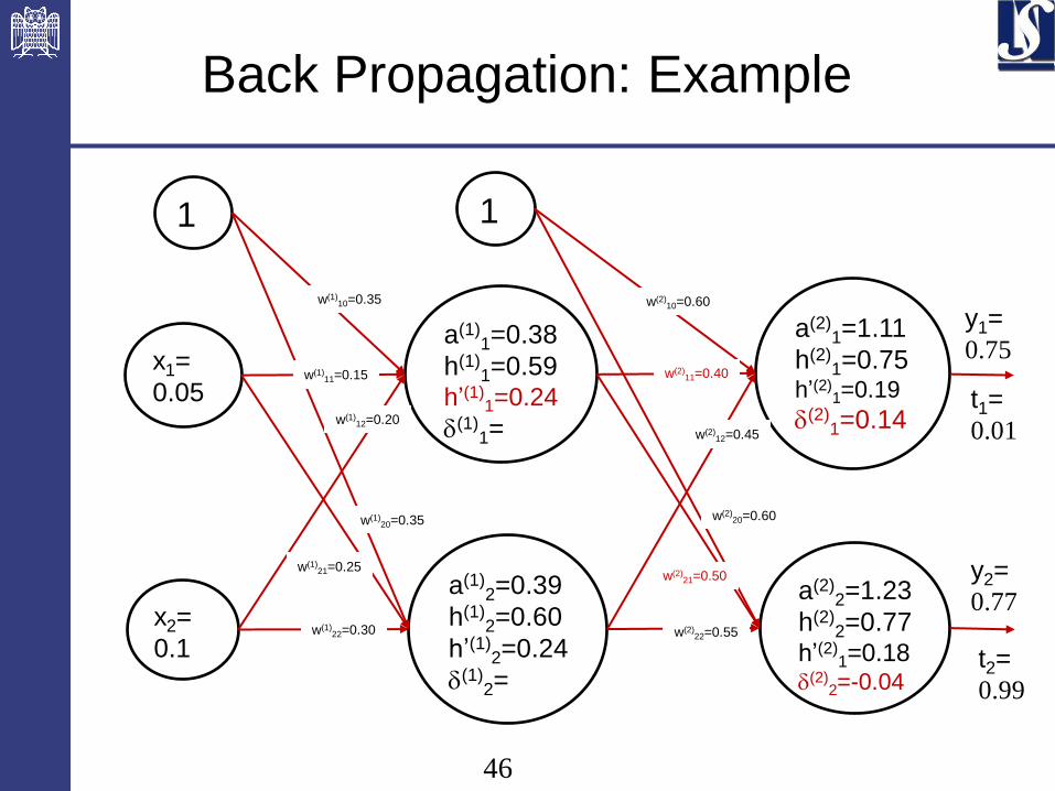
47
Back Propagation: Example
a(1)1=0.38
h(1)1=0.59
h’(1)1=0.24
d(1)1=0.01
a(1)2=0.39
h(1)2=0.60
h’(1)2=0.24
d(1)2=
a(2)1=1.11
h(2)1=0.75
h’(2)1=0.19
d(2)1=0.14
a(2)2=1.23
h(2)2=0.77
h’(2)1=0.18
d(2)2=-0.04
x1=
0.05
x2=
0.1
1 1
w(1)11=0.15
w(1)12=0.20
w(1)10=0.35
w(1)21=0.25
w(1)22=0.30
w(1)20=0.35
w(2)11=0.40
w(2)12=0.45
w(2)10=0.60
w(2)21=0.50
w(2)22=0.55
w(2)20=0.60
y1=
0.75
y2=
0.77
t1=
0.01
t2=
0.99

48
Back Propagation: Example
a(1)1=0.38
h(1)1=0.59
h’(1)1=0.24
d(1)1=0.01
a(1)2=0.39
h(1)2=0.60
h’(1)2=0.24
d(1)2=
a(2)1=1.11
h(2)1=0.75
h’(2)1=0.19
d(2)1=0.14
a(2)2=1.23
h(2)2=0.77
h’(2)1=0.18
d(2)2=-0.04
x1=
0.05
x2=
0.1
1 1
w(1)11=0.15
w(1)12=0.20
w(1)10=0.35
w(1)21=0.25
w(1)22=0.30
w(1)20=0.35
w(2)11=0.40
w(2)12=0.45
w(2)10=0.60
w(2)21=0.50
w(2)22=0.55
w(2)20=0.60
y1=
0.75
y2=
0.77
t1=
0.01
t2=
0.99
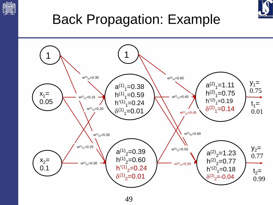
49
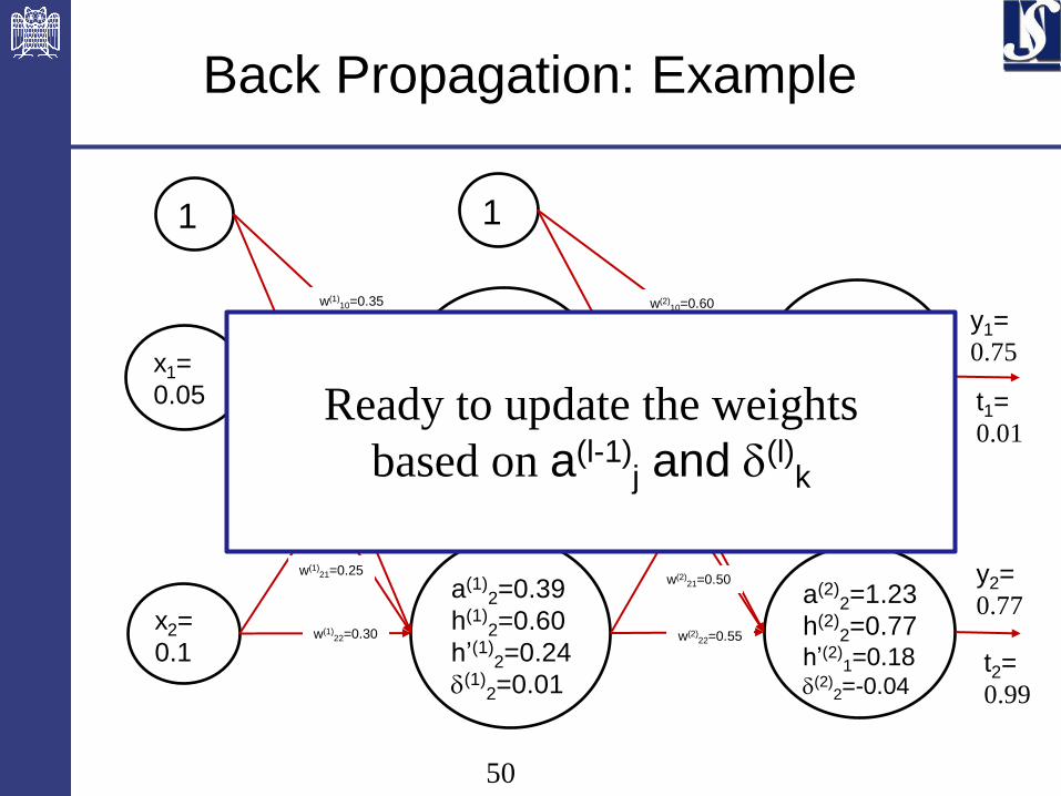
Back Propagation: Example
a(1)1=0.38
h(1)1=0.59
h’(1)1=0.24
d(1)1=0.01
a(1)2=0.39
h(1)2=0.60
h’(1)2=0.24
d(1)2=0.01
a(2)1=1.11
h(2)1=0.75
h’(2)1=0.19
d(2)1=0.14
a(2)2=1.23
h(2)2=0.77
h’(2)1=0.18
d(2)2=-0.04
x1=
0.05
x2=
0.1
1 1
w(1)11=0.15
w(1)12=0.20
w(1)10=0.35
w(1)21=0.25
w(1)22=0.30
w(1)20=0.35
w(2)11=0.40
w(2)12=0.45
w(2)10=0.60
w(2)21=0.50
w(2)22=0.55
w(2)20=0.60
y1=
0.75
y2=
0.77
t1=
0.01
t2=
0.99
50
Back Propagation: Example
a(1)1=0.38
h(1)1=0.59
h’(1)1=0.24
d(1)1=0.01
a(1)2=0.39
h(1)2=0.60
h’(1)2=0.24
d(1)2=0.01
a(2)1=1.11
h(2)1=0.75
h’(2)1=0.19
d(2)1=0.14
a(2)2=1.23
h(2)2=0.77
h’(2)1=0.18
d(2)2=-0.04
x1=
0.05
x2=
0.1
1 1
w(1)11=0.15
w(1)12=0.20
w(1)10=0.35
w(1)21=0.25
w(1)22=0.30
w(1)20=0.35
w(2)11=0.40
w(2)12=0.45
w(2)10=0.60
w(2)21=0.50
w(2)22=0.55
w(2)20=0.60
y1=
0.75
y2=
0.77
t1=
0.01
t2=
0.99
Ready to update the weights
based on a(l-1)j and d(l)
k
51
9.4 Regularization
52
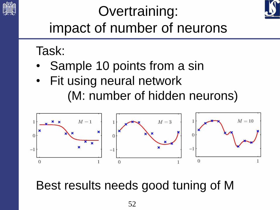
Overtraining:
impact of number of neurons
Task:
• Sample 10 points from a sin
• Fit using neural network
(M: number of hidden neurons)
Best results needs good tuning of M
53
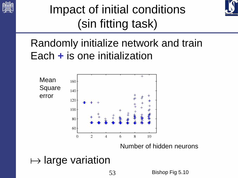
Randomly initialize network and train
Each + is one initialization
a large variation
Impact of initial conditions
(sin fitting task)
Mean
Square
error
Bishop Fig 5.10
Number of hidden neurons
54
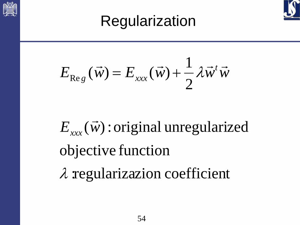
Regularization
tcoefficienzion regulariza:
function objective
zedunregulari original :)(
2
1)()(Re
wE
wwwEwE
xxx
t
xxxg
55
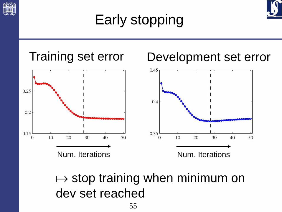
Early stopping
Training set error Development set error
Num. Iterations Num. Iterations
a stop training when minimum on
dev set reached
56
Different Methods to use Invariances
• Augment training data with
modified replica
• Specific regularization that penalizes
changes in model when input is transformed
• Build invariances into feature extraction
57
9.5 Other Types of Neural Networks and
Applications
58
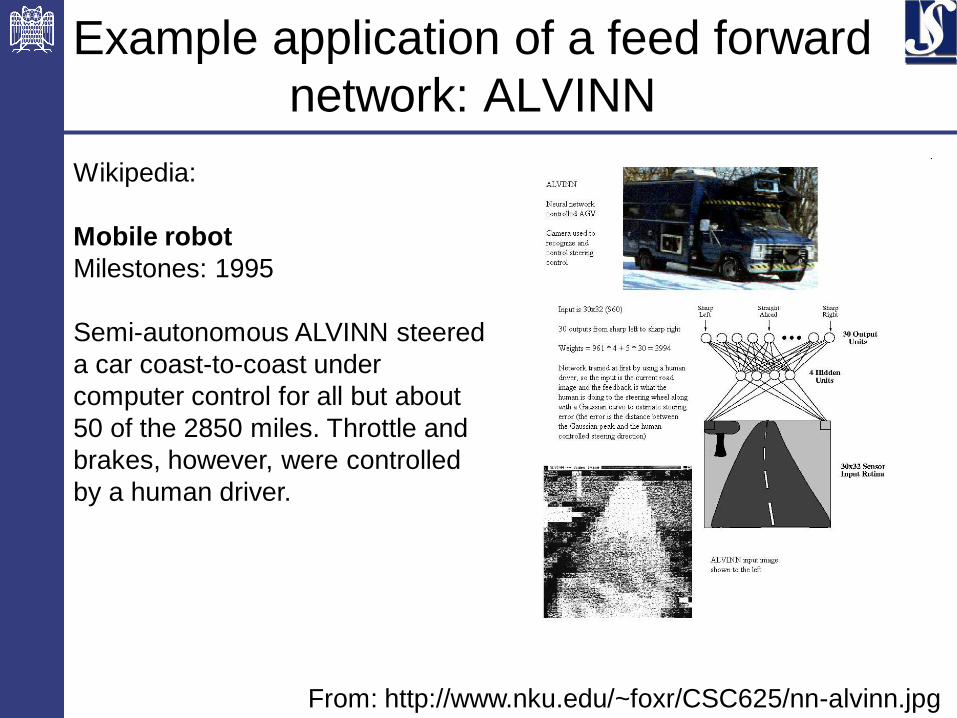
Example application of a feed forward
network: ALVINN
From: http://www.nku.edu/~foxr/CSC625/nn-alvinn.jpg
Wikipedia:
Mobile robot
Milestones: 1995
Semi-autonomous ALVINN steered
a car coast-to-coast under
computer control for all but about
50 of the 2850 miles. Throttle and
brakes, however, were controlled
by a human driver.
59
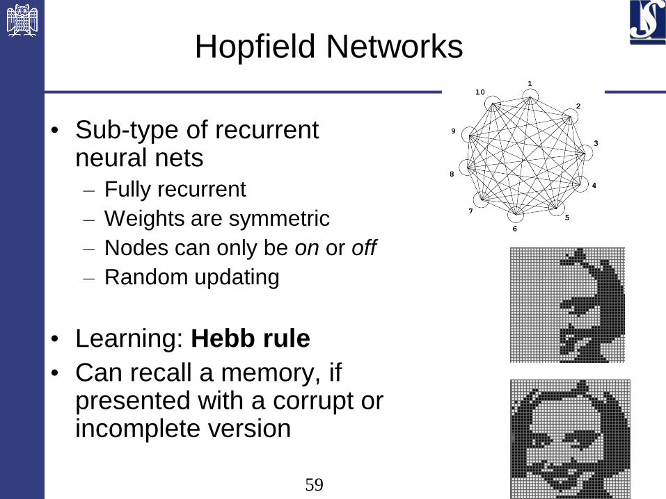
Hopfield Networks
• Sub-type of recurrent neural nets – Fully recurrent
– Weights are symmetric
– Nodes can only be on or off
– Random updating
• Learning: Hebb rule
• Can recall a memory, if presented with a corrupt or incomplete version
auto-associative or
content-addressable memory
60
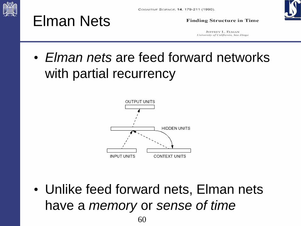
Elman Nets
• Elman nets are feed forward networks
with partial recurrency
• Unlike feed forward nets, Elman nets
have a memory or sense of time
61
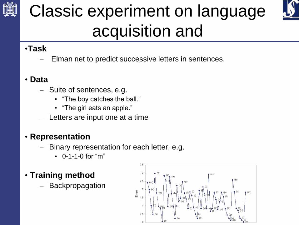
Classic experiment on language
acquisition and •Task
– Elman net to predict successive letters in sentences.
• Data
– Suite of sentences, e.g.
• “The boy catches the ball.”
• “The girl eats an apple.”
– Letters are input one at a time
• Representation
– Binary representation for each letter, e.g.
• 0-1-1-0 for “m”
• Training method
– Backpropagation

62
Classic experiment on language
acquisition and •Task
– Elman net to predict successive letters in sentences.
• Data
– Suite of sentences, e.g.
• “The boy catches the ball.”
• “The girl eats an apple.”
– Letters are input one at a time
• Representation
– Binary representation for each letter, e.g.
• 0-1-1-0 for “m”
• Training method
– Backpropagation
63
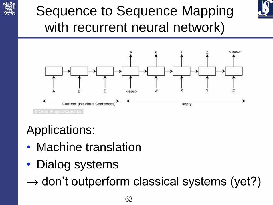
Sequence to Sequence Mapping
with recurrent neural network)
Applications:
• Machine translation
• Dialog systems
a don’t outperform classical systems (yet?)
64
Software
Theano
(https://github.com/Theano/Theano )
• extension on python
• provides symbolic differentiation
• Lot’s of example neural network implementations
Keras (http://keras.io/ )
• Builds on top of Theano
• Just specify your neural network layers
65
Summary
• Model of a neuron
• Feed forward networks
• Can model any decision boundary in
principle
• Training: back propagation
• Other networks
• Hopfield
• Elman
• Sequence-to-sequence mapping


![Deep Parametric Continuous Convolutional Neural Networks€¦ · Graph Neural Networks: Graph neural networks (GNNs) [25] are generalizations of neural networks to graph structured](https://img.pdfslide.net/doc/110x75/5f7096c356401635d36dbe30/deep-parametric-continuous-convolutional-neural-networks-graph-neural-networks.jpg)