Embed Size (px)
Citation preview
218 VOLUME 17J O U R N A L O F C L I M A T E
q 2004 American Meteorological Society
A 15-Year Climatology of Warm Conveyor Belts
SABINE ECKHARDT AND ANDREAS STOHL*
Department of Ecology, Technical University of Munich, Freising-Weihenstephan, Germany
HEINI WERNLI
Institute for Atmospheric and Climate Science, ETH Zurich, Zurich, Switzerland
PAUL JAMES, CAROLINE FORSTER, AND NICOLE SPICHTINGER
Department of Ecology, Technical University of Munich, Freising-Weihenstephan, Germany
(Manuscript received 2 January 2003, in final form 16 June 2003)
ABSTRACT
This study presents the first climatology of so-called warm conveyor belts (WCBs), strongly ascending moistairstreams in extratropical cyclones that, on the time scale of 2 days, rise from the boundary layer to the uppertroposphere. The climatology was constructed by using 15 yr (1979–93) of reanalysis data and calculating 355million trajectories starting daily from a 18 3 18 global grid at 500 m above ground level (AGL). WCBs weredefined as those trajectories that, during a period of 2 days, traveled northeastward and ascended by at least60% of the zonally and climatologically averaged tropopause height. The mean specific humidity at WCB startingpoints in different regions varies from 7 to 12 g kg21. This moisture is almost entirely precipitated out, leadingto an increase of potential temperature of 15–22 K along a WCB trajectory. Over the course of 3 days, a WCBtrajectory produces, on average, about four (six) times as much precipitation as a global (extratropical) averagetrajectory starting from 500 m AGL. WCB starting points are most frequently located between approximately258 and 458N and between about 208 and 458S. In the Northern Hemisphere (NH), there are two distinct frequencymaxima east of North America and east of Asia, whereas there is much less zonal variability in the SouthernHemisphere (SH). In the NH, WCBs are almost an order of magnitude more frequent in January than in July,whereas in the SH the seasonal variation is much weaker. In order to study the relationship between WCBs andcyclones, an independent cyclone climatology was used. Most of the WCBs were found in the vicinity of acyclone center, whereas the reverse comparison revealed that cyclones are normally accompanied by a strongWCB only in the NH winter. In the SH, this is not the case throughout the year. Particularly around Antarctica,where cyclones are globally most frequent, practically no strong WCBs are found. These cyclones are lessinfluenced by diabatic processes and, thus, they are associated with fewer high clouds and less precipitationthan cyclones in other regions. In winter, there is a highly significant correlation between the North AtlanticOscillation (NAO) and the WCB distribution in the North Atlantic: In months with a high NAO index, WCBsare about 12% more frequent and their outflow occurs about 108 latitude farther north and 208 longitude farthereast than in months with a low NAO index. The differences in the WCB inflow regions are relatively smallbetween the two NAO phases. During high phases of the Southern Oscillation, WCBs occur more (less) frequentaround Australia (in the South Atlantic).
1. Introduction
The global atmospheric circulation is characterizedby the poleward transport of energy in terms of bothsensible and latent heat (Peixoto and Oort 1992). In theTropics, where the Coriolis force is small, the energy
* Current affiliation: CIRES, University of Colorado/NOAA Aer-onomy Laboratory, Boulder, Colorado.
Corresponding author address: Sabine Eckhardt, Department ofEcology, Technical University of Munich, Am Hochanger 13, D-85354 Freising-Weihenstephan, Germany.E-mail: [email protected]
transport is accomplished via zonally almost symmetricconvective overturning, that is, the Hadley cell. Outsidethe Tropics, a westerly thermal wind is established be-tween the warmer low latitudes and the colder highlatitudes. Such a jetlike flow is baroclinically unstable,resulting in baroclinic waves transporting the energypoleward. Essential features of these baroclinic wavesare the embedded cyclones and anticyclones that ac-count for most of the atmospheric variability in the mid-latitudes on synoptic time scales (Trenberth 1991). Thefronts associated with the cyclones are particularly note-worthy, as they produce a major fraction of both theupward and poleward moisture transport and the pre-
1 JANUARY 2004 219E C K H A R D T E T A L .
cipitation in the midlatitudes (Stewart et al. 1998). Baro-clinic waves are also important for the transport ofchemical trace constituents in the atmosphere (Wang andShallcross 2000). Furthermore, extratropical cyclonesvent the atmospheric boundary layer (ABL) (Cotton etal. 1995) and, thus, are crucial for cleansing the ABLfrom air pollution and aerosols.
Since cyclones are such an important component ofthe climate system, it is not surprising that much efforthas been put into the characterization of their geograph-ical distribution. Because of the location of landmasses,it is far from zonal uniformity, in particular in the North-ern Hemisphere (NH), where cyclones are concentratedover the Atlantic and Pacific Oceans (Gulev et al. 2001;Sickmoller et al. 2000; Hoskins and Hodges 2002). Inthe Southern Hemisphere (SH), the cyclone distributionshows less zonal variability (Sinclair 1994; Simmondsand Keay 2000a,b).
Different methods exist for constructing cyclone cli-matologies, most of which diagnose cyclone centers(e.g., by identifying pressure or geopotential height min-ima at various levels in the troposphere, or relative vor-ticity maxima in the lower troposphere) and track themover the cyclone’s life cycle [see Hoskins and Hodges(2002), for a comparison of some techniques]. However,technical problems exist with these methods (e.g., un-realistic reduction of pressure to sea level over topog-raphy, ambiguous tracking algorithms). Thus, it is notsurprising that existing cyclone climatologies are inmodest agreement with each other, particularly in theSH. Many of the identified structures may be heat lowsor lee troughs that have limited vertical extent and arenot associated with deep clouds or significant amountsof precipitation (Sinclair 1994). Furthermore, there isno simple relation between, say, the depth of a surfacepressure minimum and important properties of the cor-responding cyclone (e.g., its transport of heat, watervapor, and trace gases, or cloud and rain formation). Forinstance, Martin (1998) and Iskenderian (1988) dis-cussed the case of a very modest surface cyclone, whichproduced extremely heavy snowfall over North Amer-ica. This limits the significance of existing cyclone cli-matologies. An attractive alternative to these climatol-ogies therefore would be to diagnose, instead, directlythose airstreams that produce the largest portion of acyclone’s precipitation and cause most of its meridionalheat transport.
The study of airflows associated with extratropicalcyclones has a long history and goes back to the de-velopment of the Bergen school cyclone model (e.g.,Bjerknes 1910). Later, the quasi-Lagrangian conveyorbelt model was developed by Harrold (1973), Browninget al. (1973), and Carlson (1980) (see also Browning1990, 1999; Carlson 1998). This model describes threeairstreams in a coordinate system moving with the cy-clone. They are typically of the order of 1 km in depthand a few hundred kilometers across. The dry intrusion(DI) descends behind the cold front from the upper tro-
posphere and/or lower stratosphere to the lower tro-posphere. The cold conveyor belt (CCB) splits into twobranches; an anticyclonic branch, which ascends aheadof the surface warm front from the ABL into the middletroposphere and a cyclonic branch, which remains inthe lower troposphere (Schultz 2001). The warm con-veyor belt (WCB), experiencing the strongest verticalmotion of the three airstreams, ascends slantwise aheadof the surface cold front from the ABL all the way intothe upper troposphere, where it may override the CCB.The WCB originates in the cyclone’s warm sector andis responsible for most of the cyclone’s meridional en-ergy transport, in terms of both latent and sensible heat.In infrared satellite images, WCBs are clearly visible asbright frontal cloud bands, which forecasters associatewith maturing cyclones. WCBs furthermore appear asso-called atmospheric rivers in global maps of the ver-tically integrated water vapor flux, with a water flowcomparable to that of the Amazon (Newell et al. 1992).
From a dynamical standpoint, WCBs are importantfor the evolution of the cyclone they pertain to, for thepotential formation of downstream upper-level anticy-clones, and for the rapid transport of ABL air into theupper troposphere and lowermost stratosphere (Wernliand Bourqui 2002). WCBs constitute a Lagrangian man-ifestation of the impact of latent heat release on cyclonedevelopment. The general picture is that condensationalheating leads to the production of positive potential vor-ticity (PV) anomalies in the lower/middle troposphere(e.g., Stoelinga 1996; Wernli and Davies 1997) and fi-nally to an enhancement of cyclone development thatis otherwise determined by dry dynamics (e.g., Kuo etal. 1991; Davis et al. 1993). WCBs also develop inmodel simulations with dry dynamics only, but theseare less strong than when also moist processes are ac-counted for. This suggests that the occurrence of a prom-inent WCB in the vicinity of an extratropical cyclonehints at a rapid storm development, potentially also lead-ing to explosive genesis of so-called bombs (Sandersand Gyakum 1980; Zhu and Newell 1994). It will there-fore be of interest to verify whether WCBs are mostfrequent in regions of preferred rapid cyclogenesis. Alsoof relevance are the upper-level effects induced byWCBs. After the ascent phase, WCBs arrive in the uppertroposphere with low tropospheric PV values (typically,0.6 PV units; Wernli 1997; Pomroy and Thorpe 2000).At the level of the WCB outflow, these values can cor-respond to significant negative PV anomalies in the up-per troposphere. Low-PV air masses in the upper tro-posphere are important, for instance, for maintainingblocking (e.g., Mullen 1987), and C. B. Schwierz et al.(2003, unpublished manuscript) identified the signifi-cant role of PV modification in WCBs for the sustenanceof North Atlantic blocking. Massacand et al. (2001) pre-sented a case where the upper-level anticyclonic flow,enhanced by the outflow of a WCB, contributed to thedownstream formation of a PV streamer. Some of the
220 VOLUME 17J O U R N A L O F C L I M A T E
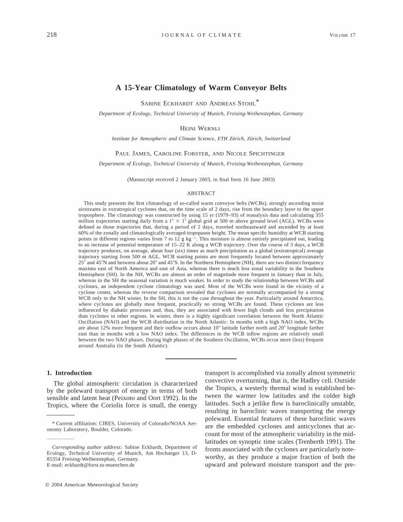
FIG. 1. Zonally averaged tropopause height (gray line) and 60%of the zonally averaged tropopause height (black line) as a functionof latitude.
WCB outflow can enter the stratosphere during the daysafter the ascent (Stohl 2001). The physical processesleading to the associated PV increase are not yet fullyunderstood, but one hypothesis is that radiation inducessignificant PV changes near the maximum vertical mois-ture gradient (Zierl and Wirth 1997).
Large differences also exist between the chemicalcharacteristics of the airstreams in a cyclone (Bethan etal. 1998), leading to an extension of the conceptual con-veyor belt model to include also the airstream’s chemicalcomposition (Cooper et al. 2001, 2002). Recently,WCBs have been found to be important for the long-range transport of air pollution, for instance, intercon-tinental transport of sulfur (Arnold et al. 1997), ozone(Stohl and Trickl 1999), and ozone precursors (Stohl etal. 2003). WCBs transport these substances to the tro-popause region, thus enhancing possible effects on theradiative forcing of the earth–atmosphere system. Theyalso influence the formation and properties of cirrusclouds through the upward transport of both moistureand ice nuclei (Rogers et al. 1998), may trigger ion-induced nucleation of aerosols (Stohl et al. 2003), andfavor the development of contrails (Kastner et al. 1999).Thus, WCBs have tremendous effects not only on theatmospheric energy and moisture budgets, but on theclimate system as a whole. Despite their great impor-tance, no attempt has been made yet to determine theirglobal geographical distribution over longer time peri-ods. In this paper, we present a first 15-yr climatologyof WCBs using meteorological reanalysis data.
One method to diagnose WCBs in global meteoro-logical datasets uses trajectories, which emphasizes theirLagrangian nature. In case studies, Wernli and Davies(1997) and Wernli (1997) have shown that WCBs areassociated with coherent ensembles of trajectories withcharacteristic properties (e.g., strong ascent, strong de-crease in water vapor and corresponding increase inpotential temperature, poleward and eastward motion)that can be used to diagnose WCBs in a global trajectorydataset. Stohl (2001) has used this method to establisha first 1-yr ‘‘climatology’’ of WCBs and other airstreamsin the NH, which revealed two maxima in the frequencyof WCB inflow, located south of the entrance to the twostorm tracks.
In this paper we extend Stohl’s (2001) study to bothhemispheres and a 15-yr period, and develop a detailedcharacterization of WCBs. In section 2 we explain ourWCB identification procedure and demonstrate it in acase study. In section 3 we discuss the main propertiesof WCBs and present their 15-yr climatology, whichthen is compared with a cyclone climatology in section4. In section 5 we examine the relationship betweenWCBs and precipitation. The interannual variability ofWCB occurrence, and its relationship to important mea-sures of climate variability, is studied in section 6. Fi-nally, conclusions are drawn in section 7.
2. Methods and an illustrating case study
a. Trajectory calculations
Three-dimensional trajectory calculations were car-ried out with the Lagrangian model FLEXTRA (Stohlet al. 1995; Stohl and Seibert 1998), which is used withwind fields from the European Centre for Medium-Range Weather Forecasts (ECMWF). Details on FLEX-TRA can be obtained online (at http://www.forst.tu-muenchen.de/EXT/LST/METEO/stohl/flextra.html).An intercomparison of FLEXTRA with other trajectorymodels can be found in Stohl et al. (2001). For thisstudy we have used the ECMWF 15-yr re-analysis da-taset (ERA-15), which was produced with a T106 spec-tral model (Gibson et al. 1999) and covers the yearsfrom 1979 to 1993. We retrieved these data from theECMWF archives with a resolution of 18 3 18, 31 levels,and every 6 h. Six-day forward trajectories were startedat 500 m AGL on a global grid of 18 3 18 resolutionat 1200 UTC every day, which gives a total number of355 million trajectories. The model output consisted ofthe trajectory positions, and values of PV, potential tem-perature Q, specific humidity q, and pressure along thetrajectories every 24 h.
b. WCB selection criteria
As seen in a case study presented below and in Wernliand Davies (1997), the trajectories associated with aWCB are characterized by rapid ascent and transportfirst poleward, and then eastward within about two days.We used these features to identify WCBs automaticallyin the 15-yr global dataset. A trajectory was classifiedas a WCB trajectory if, during the first 2 days, it traveledmore than 108 longitude to the east and more than 58latitude to the north, and ascended by more than 60%of the zonally and climatologically averaged tropopauseheight at the trajectory’s latitudinal position after 2 days.This accounts for the fact that WCBs start in the ABLand rise within about two days to the upper troposphere.
Zonal mean tropopause heights were calculated from
1 JANUARY 2004 221E C K H A R D T E T A L .
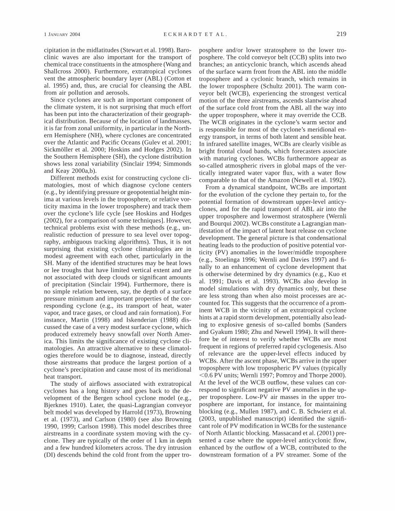
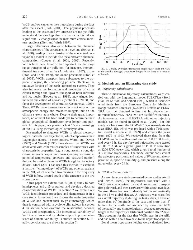
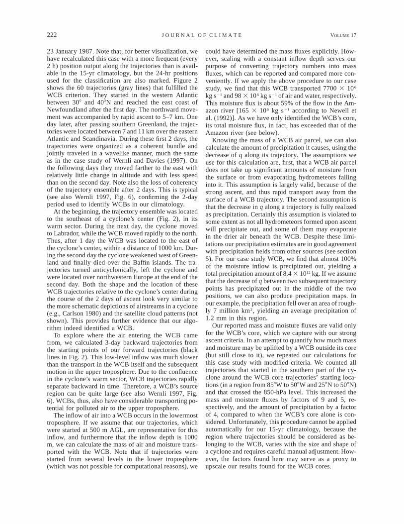
FIG. 2. Six-day trajectories starting 1200 UTC 23 Jan 1987, of which the first 2 days wereidentified as a WCB. (a) The forward trajectories (gray) and 3-day backward trajectories (black)from the starting locations of the forward trajectories. Positions along the forward trajectories aremarked every 24 h. Sea level pressure (light gray) contour lines are drawn every 10 hPa for thetrajectory starting time (1200 UTC 23 Jan 1987). For clarity, only those WCB trajectories as-sociated with the cyclone over the eastern seaboard of North America are drawn. (b) Verticalprojection of the trajectories shown in (a).
the ECMWF data and are shown as a function of latitudein Fig. 1. A thermal tropopause criterion (WMO 1957)was used in the Tropics (208S to 208N) and a dynamicalone (2 PV units) poleward of 308 (Hoskins et al. 1985),respectively. In the region between 6208 and 6308 weinterpolated between the thermal and the dynamical tro-popause linearly. In the midlatitudes the threshold heightfor WCB trajectories after 2 days varies from about 8(308) to 5 km (.608).
Any criterion used for an automatic classification ofWCBs is necessarily subjective. We designed our cri-teria to be conservative in a sense that only the coresof reasonably strong WCBs shall be identified, whereastrajectories close to the airstream’s boundaries—whererapid dispersion occurs (Cohen and Kreitzberg 1997)—and also weak WCBs shall not be identified. However,while the absolute number of WCB trajectories is highlysensitive to variations of our criteria, the identified spa-tial patterns of WCB frequency are very robust. Stohl(2001) used a constant ascent criterion of 8000 m insteadof the one used here, which depends on the latitude,causing a tendency to underestimate the frequency ofWCBs at high latitudes. However, even with Stohl’s
(2001) criteria the identified spatial patterns were quitesimilar. The criteria requiring a northward and eastwardmotion are effective in preventing airstreams in theTropics from being misclassified as WCBs and wereused already by Stohl (2001). The algorithm may oc-casionally miss cyclonically turning WCBs, in particular‘‘trowal’’-type airstreams, which can turn westward(Martin 1998), at least in a quasi-Lagrangian coordinatesystem moving with the cyclone. But over the time pe-riod of 2 days and in an absolute coordinate systemeven those airstreams often travel sufficiently far to theeast in order to be correctly classified as WCBs. In fact,imposing the eastward-moving criterion leads to a glob-al reduction of the WCB mass fluxes of only 20%, com-pared to a doubling for a reduction of the ascent criterionby 10%. However, without this criterion, sometimestropical airstreams (e.g., in hurricanes) would have beenmisclassifed as WCBs.
c. A case study example
To illustrate our methodology, we present a typicalexample of a WCB occurring in the North Atlantic on
222 VOLUME 17J O U R N A L O F C L I M A T E
23 January 1987. Note that, for better visualization, wehave recalculated this case with a more frequent (every2 h) position output along the trajectories than is avail-able in the 15-yr climatology, but the 24-hr positionsused for the classification are also marked. Figure 2shows the 60 trajectories (gray lines) that fulfilled theWCB criterion. They started in the western Atlanticbetween 308 and 408N and reached the east coast ofNewfoundland after the first day. The northward move-ment was accompanied by rapid ascent to 5–7 km. Oneday later, after passing southern Greenland, the trajec-tories were located between 7 and 11 km over the easternAtlantic and Scandinavia. During these first 2 days, thetrajectories were organized as a coherent bundle andjointly traveled in a wavelike manner, much the sameas in the case study of Wernli and Davies (1997). Onthe following days they moved farther to the east withrelatively little change in altitude and with less speedthan on the second day. Note also the loss of coherencyof the trajectory ensemble after 2 days. This is typical(see also Wernli 1997, Fig. 6), confirming the 2-dayperiod used to identify WCBs in our climatology.
At the beginning, the trajectory ensemble was locatedto the southeast of a cyclone’s center (Fig. 2), in itswarm sector. During the next day, the cyclone movedto Labrador, while the WCB moved rapidly to the north.Thus, after 1 day the WCB was located to the east ofthe cyclone’s center, within a distance of 1000 km. Dur-ing the second day the cyclone weakened west of Green-land and finally died over the Baffin islands. The tra-jectories turned anticyclonically, left the cyclone andwere located over northwestern Europe at the end of thesecond day. Both the shape and the location of theseWCB trajectories relative to the cyclone’s center duringthe course of the 2 days of ascent look very similar tothe more schematic depictions of airstreams in a cyclone(e.g., Carlson 1980) and the satellite cloud patterns (notshown). This provides further evidence that our algo-rithm indeed identified a WCB.
To explore where the air entering the WCB camefrom, we calculated 3-day backward trajectories fromthe starting points of our forward trajectories (blacklines in Fig. 2). This low-level inflow was much slowerthan the transport in the WCB itself and the subsequentmotion in the upper troposphere. Due to the confluencein the cyclone’s warm sector, WCB trajectories rapidlyseparate backward in time. Therefore, a WCB’s sourceregion can be quite large (see also Wernli 1997, Fig.6). WCBs, thus, also have considerable transporting po-tential for polluted air to the upper troposphere.
The inflow of air into a WCB occurs in the lowermosttroposphere. If we assume that our trajectories, whichwere started at 500 m AGL, are representative for thisinflow, and furthermore that the inflow depth is 1000m, we can calculate the mass of air and moisture trans-ported with the WCB. Note that if trajectories werestarted from several levels in the lower troposphere(which was not possible for computational reasons), we
could have determined the mass fluxes explicitly. How-ever, scaling with a constant inflow depth serves ourpurpose of converting trajectory numbers into massfluxes, which can be reported and compared more con-veniently. If we apply the above procedure to our casestudy, we find that this WCB transported 7700 3 106
kg s21 and 98 3 106 kg s21 of air and water, respectively.This moisture flux is about 59% of the flow in the Am-azon river [165 3 106 kg s21 according to Newell etal. (1992)]. As we have only identified the WCB’s core,its total moisture flux, in fact, has exceeded that of theAmazon river (see below).
Knowing the mass of a WCB air parcel, we can alsocalculate the amount of precipitation it causes, using thedecrease of q along its trajectory. The assumptions weuse for this calculation are, first, that a WCB air parceldoes not take up significant amounts of moisture fromthe surface or from evaporating hydrometeors fallinginto it. This assumption is largely valid, because of thestrong ascent, and thus rapid transport away from thesurface of a WCB trajectory. The second assumption isthat the decrease in q along a trajectory is fully realizedas precipitation. Certainly this assumption is violated tosome extent as not all hydrometeors formed upon ascentwill precipitate out, and some of them may evaporatein the drier air beneath the WCB. Despite these limi-tations our precipitation estimates are in good agreementwith precipitation fields from other sources (see section5). For our case study WCB, we find that almost 100%of the moisture inflow is precipitated out, yielding atotal precipitation amount of 8.4 3 1012 kg. If we assumethat the decrease of q between two subsequent trajectorypoints has precipitated out in the middle of the twopositions, we can also produce precipitation maps. Inour example, the precipitation fell over an area of rough-ly 7 million km2, yielding an average precipitation of1.2 mm in this region.
Our reported mass and moisture fluxes are valid onlyfor the WCB’s core, which we capture with our strongascent criteria. In an attempt to quantify how much massand moisture may be uplifted by a WCB outside its core(but still close to it), we repeated our calculations forthis case study with modified criteria. We counted alltrajectories that started in the southern part of the cy-clone around the WCB core trajectories’ starting loca-tions (in a region from 858W to 508W and 258N to 508N)and that crossed the 850-hPa level. This increased themass and moisture fluxes by factors of 9 and 5, re-spectively, and the amount of precipitation by a factorof 4, compared to when the WCB’s core alone is con-sidered. Unfortunately, this procedure cannot be appliedautomatically for our 15-yr climatology, because theregion where trajectories should be considered as be-longing to the WCB, varies with the size and shape ofa cyclone and requires careful manual adjustment. How-ever, the factors found here may serve as a proxy toupscale our results found for the WCB cores.
1 JANUARY 2004 223E C K H A R D T E T A L .
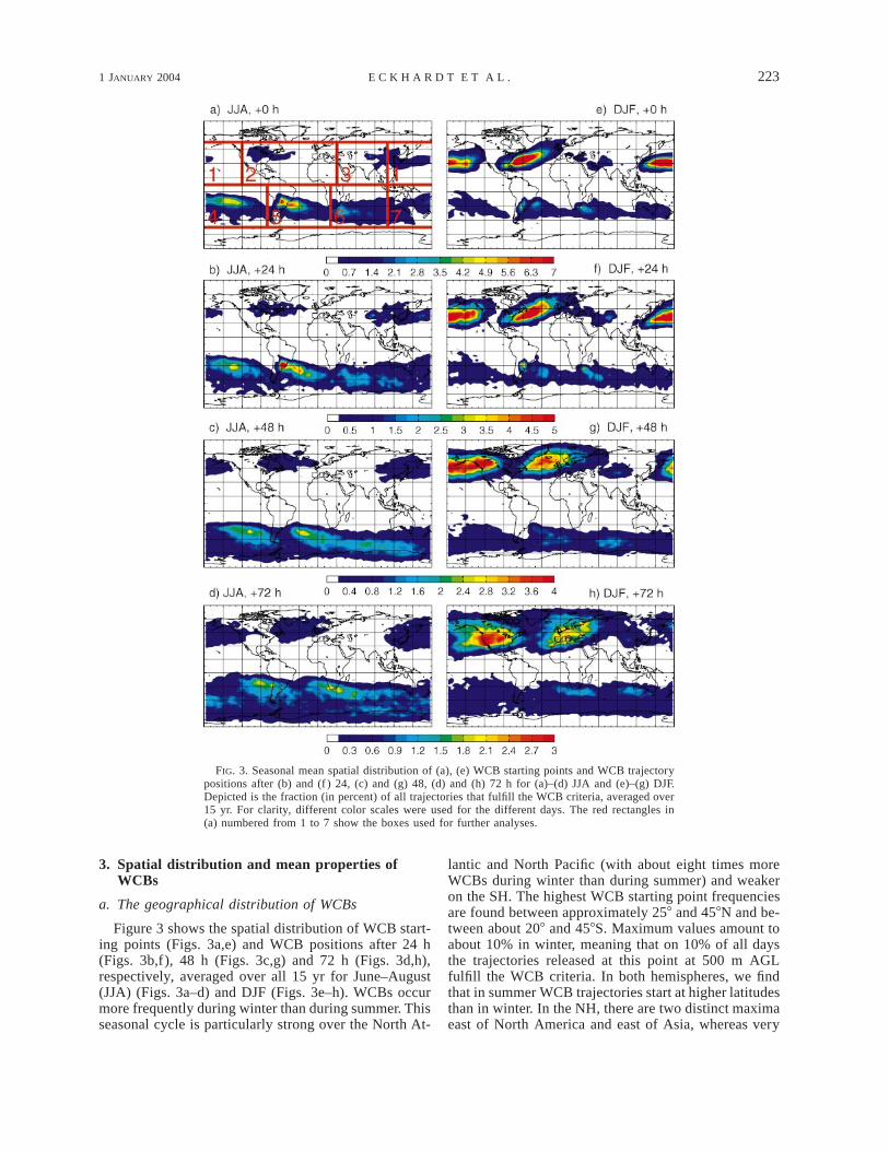
FIG. 3. Seasonal mean spatial distribution of (a), (e) WCB starting points and WCB trajectorypositions after (b) and (f ) 24, (c) and (g) 48, (d) and (h) 72 h for (a)–(d) JJA and (e)–(g) DJF.Depicted is the fraction (in percent) of all trajectories that fulfill the WCB criteria, averaged over15 yr. For clarity, different color scales were used for the different days. The red rectangles in(a) numbered from 1 to 7 show the boxes used for further analyses.
3. Spatial distribution and mean properties ofWCBs
a. The geographical distribution of WCBs
Figure 3 shows the spatial distribution of WCB start-ing points (Figs. 3a,e) and WCB positions after 24 h(Figs. 3b,f), 48 h (Figs. 3c,g) and 72 h (Figs. 3d,h),respectively, averaged over all 15 yr for June–August(JJA) (Figs. 3a–d) and DJF (Figs. 3e–h). WCBs occurmore frequently during winter than during summer. Thisseasonal cycle is particularly strong over the North At-
lantic and North Pacific (with about eight times moreWCBs during winter than during summer) and weakeron the SH. The highest WCB starting point frequenciesare found between approximately 258 and 458N and be-tween about 208 and 458S. Maximum values amount toabout 10% in winter, meaning that on 10% of all daysthe trajectories released at this point at 500 m AGLfulfill the WCB criteria. In both hemispheres, we findthat in summer WCB trajectories start at higher latitudesthan in winter. In the NH, there are two distinct maximaeast of North America and east of Asia, whereas very
224 VOLUME 17J O U R N A L O F C L I M A T E
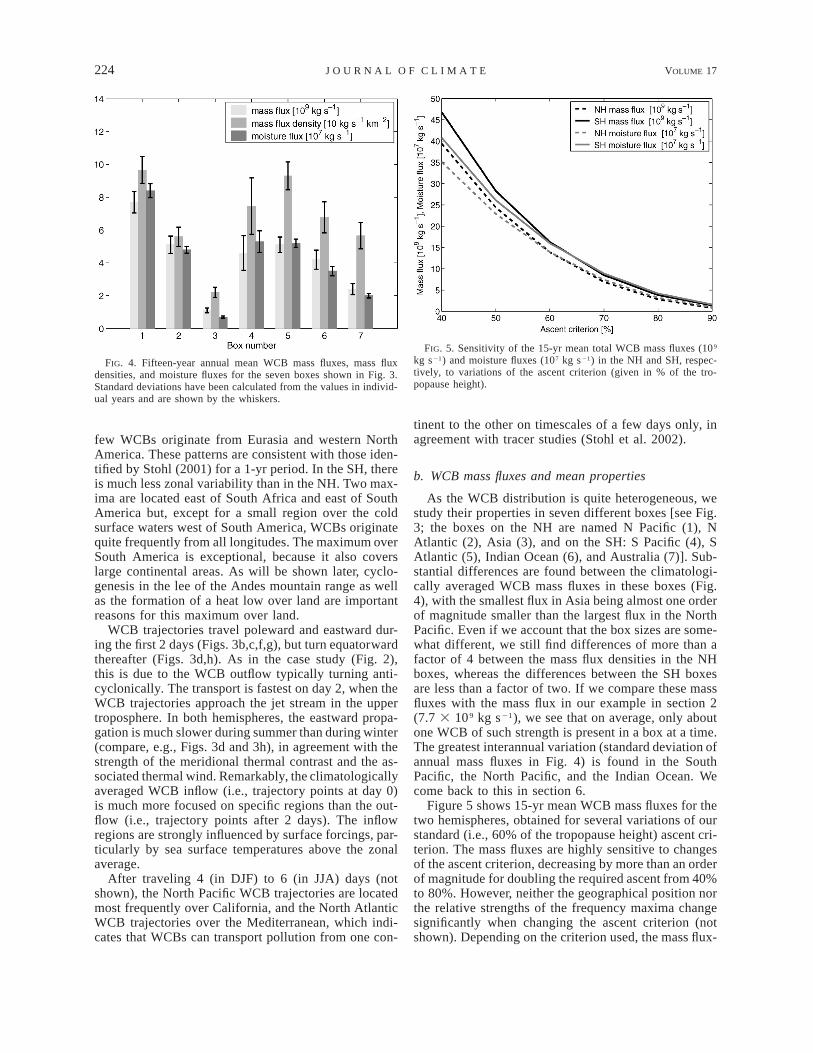
FIG. 4. Fifteen-year annual mean WCB mass fluxes, mass fluxdensities, and moisture fluxes for the seven boxes shown in Fig. 3.Standard deviations have been calculated from the values in individ-ual years and are shown by the whiskers.
FIG. 5. Sensitivity of the 15-yr mean total WCB mass fluxes (109
kg s21) and moisture fluxes (107 kg s21) in the NH and SH, respec-tively, to variations of the ascent criterion (given in % of the tro-popause height).
few WCBs originate from Eurasia and western NorthAmerica. These patterns are consistent with those iden-tified by Stohl (2001) for a 1-yr period. In the SH, thereis much less zonal variability than in the NH. Two max-ima are located east of South Africa and east of SouthAmerica but, except for a small region over the coldsurface waters west of South America, WCBs originatequite frequently from all longitudes. The maximum overSouth America is exceptional, because it also coverslarge continental areas. As will be shown later, cyclo-genesis in the lee of the Andes mountain range as wellas the formation of a heat low over land are importantreasons for this maximum over land.
WCB trajectories travel poleward and eastward dur-ing the first 2 days (Figs. 3b,c,f,g), but turn equatorwardthereafter (Figs. 3d,h). As in the case study (Fig. 2),this is due to the WCB outflow typically turning anti-cyclonically. The transport is fastest on day 2, when theWCB trajectories approach the jet stream in the uppertroposphere. In both hemispheres, the eastward propa-gation is much slower during summer than during winter(compare, e.g., Figs. 3d and 3h), in agreement with thestrength of the meridional thermal contrast and the as-sociated thermal wind. Remarkably, the climatologicallyaveraged WCB inflow (i.e., trajectory points at day 0)is much more focused on specific regions than the out-flow (i.e., trajectory points after 2 days). The inflowregions are strongly influenced by surface forcings, par-ticularly by sea surface temperatures above the zonalaverage.
After traveling 4 (in DJF) to 6 (in JJA) days (notshown), the North Pacific WCB trajectories are locatedmost frequently over California, and the North AtlanticWCB trajectories over the Mediterranean, which indi-cates that WCBs can transport pollution from one con-
tinent to the other on timescales of a few days only, inagreement with tracer studies (Stohl et al. 2002).
b. WCB mass fluxes and mean properties
As the WCB distribution is quite heterogeneous, westudy their properties in seven different boxes [see Fig.3; the boxes on the NH are named N Pacific (1), NAtlantic (2), Asia (3), and on the SH: S Pacific (4), SAtlantic (5), Indian Ocean (6), and Australia (7)]. Sub-stantial differences are found between the climatologi-cally averaged WCB mass fluxes in these boxes (Fig.4), with the smallest flux in Asia being almost one orderof magnitude smaller than the largest flux in the NorthPacific. Even if we account that the box sizes are some-what different, we still find differences of more than afactor of 4 between the mass flux densities in the NHboxes, whereas the differences between the SH boxesare less than a factor of two. If we compare these massfluxes with the mass flux in our example in section 2(7.7 3 109 kg s21), we see that on average, only aboutone WCB of such strength is present in a box at a time.The greatest interannual variation (standard deviation ofannual mass fluxes in Fig. 4) is found in the SouthPacific, the North Pacific, and the Indian Ocean. Wecome back to this in section 6.
Figure 5 shows 15-yr mean WCB mass fluxes for thetwo hemispheres, obtained for several variations of ourstandard (i.e., 60% of the tropopause height) ascent cri-terion. The mass fluxes are highly sensitive to changesof the ascent criterion, decreasing by more than an orderof magnitude for doubling the required ascent from 40%to 80%. However, neither the geographical position northe relative strengths of the frequency maxima changesignificantly when changing the ascent criterion (notshown). Depending on the criterion used, the mass flux-
1 JANUARY 2004 225E C K H A R D T E T A L .
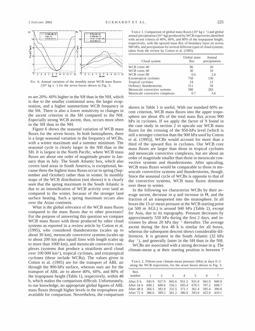
FIG. 6. Annual variation of the monthly mean WCB mass fluxes(109 kg s21) for the seven boxes shown in Fig. 3.
TABLE 1. Comparison of global mass fluxes (109 kg s21) and globalannual precipitation (1015 kg) produced by WCB trajectories identifiedwith ascent criteria of 40%, 60%, and 80% of the tropopause height,respectively, with the upward mass flux of boundary layer air across900 hPa, and precipitation for several different types of cloud systems,taken from the review by Cotton et al. (1995).
Cloud systemGlobal mass
fluxAnnual
precipitation
WCB cores 40WCB cores 60WCB cores 80Extratropical cyclonesTropical cyclones
86306.6
75024
26102.6
13012
Ordinary thunderstormsMesoscale convective systemsMesoscale convective complexes
211580
0.7
56283
3.6
TABLE 2. Fifteen-year climate-mean pressure (hPa) at days 0–3along the WCB trajectories, for the seven boxes shown in Fig. 3.
Boxnumber 1 2 3 4 5 6 7
After 0 hAfter 24 hAfter 48 hAfter 72 h
945.9690.1366.5386.6
927.9680.6382.9399.2
845.6556.1332.5361.2
951.5693.4371.1386.9
931.9670.5361.4393.0
941.9707.2395.4425.9
940.9698.7390.8410.1
es are 20%–60% higher in the SH than in the NH, whichis due to the smaller continental area, the larger evap-oration, and a higher summertime WCB frequency inthe SH. There is also a lower sensitivity to changes inthe ascent criterion in the SH compared to the NH.Especially strong WCB ascent, thus, occurs more oftenin the SH than in the NH.
Figure 6 shows the seasonal variation of WCB massfluxes for the seven boxes. In both hemispheres, thereis a large seasonal variation in the frequency of WCBs,with a winter maximum and a summer minimum. Theseasonal cycle is clearly larger in the NH than in theSH. It is largest in the North Pacific, where WCB massfluxes are about one order of magnitude greater in Jan-uary than in July. The South Atlantic box, which alsocovers land areas in South America, is exceptional, be-cause there the highest mass fluxes occur in spring (Sep-tember and October) rather than in winter. In monthlymaps of the WCB distribution (not shown) it is clearlyseen that the spring maximum in the South Atlantic isdue to an intensification of WCB activity over land ascompared to the winter, because of the stronger landsurface heating. Such a spring maximum occurs alsoover the Asian continent.
What is the global relevance of the WCB mass fluxescompared to the mass fluxes due to other processes?For the purpose of answering this question we compareWCB mass fluxes with those produced by other cloudsystems as reported in a review article by Cotton et al.(1995), who considered thunderstorms (scales up toabout 30 km), mesoscale convective systems (scales upto about 200 km plus squall lines with length scales upto more than 1000 km), and mesoscale convective com-plexes (systems that produce a stratiform anvil cloudover 100 000 km2), tropical cyclones, and extratropicalcyclones (these include WCBs). The values given inCotton et al. (1995) are for the transport of ABL airthrough the 900-hPa surface, whereas ours are for thetransport of ABL air to above 40%, 60%, and 80% ofthe tropopause height (Table 1), respectively, within 48h, which makes the comparison difficult. Unfortunately,to our knowledge, no appropriate global figures of ABLmass fluxes through higher levels in the troposphere areavailable for comparison. Nevertheless, the comparison
shown in Table 1 is useful. With our standard 60% as-cent criterion, WCB mass fluxes into the upper tropo-sphere are about 4% of the total mass flux across 900hPa in cyclones. If we apply the factor of 9 found inthe case study in section 2 to upscale our WCB massfluxes for the crossing of the 850-hPa level [which isstill a stronger criterion than the 900 hPa used by Cottonet al. (1995)], WCBs would account for more than athird of the upward flux in cyclones. Our WCB coremass fluxes are larger than those in tropical cyclonesand mesoscale convective complexes, but are about anorder of magnitude smaller than those in mesoscale con-vective systems and thunderstorms. After upscaling,WCB mass fluxes would be comparable to those in me-soscale convective systems and thunderstorms, though.Since the seasonal cycle of WCBs is opposite to that ofthe convective systems, WCB mass fluxes dominateover these in winter.
In the following we characterize WCBs by their av-erage ascent, decrease in q and increase in Q, and thefraction of air transported into the stratosphere. In allboxes the 15-yr mean pressure at the WCB starting point(at 500 m AGL) is around 940 hPa (Table 2), exceptfor Asia, due to its topography. Pressure decreases byapproximately 550 hPa during the first 2 days, and in-creases by about 20 hPa day21 thereafter. The averageascent during the first 48 h is similar for all boxes,whereas the subsequent descent shows considerable dif-ferences. It is greatest in the South Atlantic (32 hPaday21), and generally faster in the SH than in the NH.
WCBs are associated with a strong decrease in q. Theclimate-mean q at their starting position is between 7
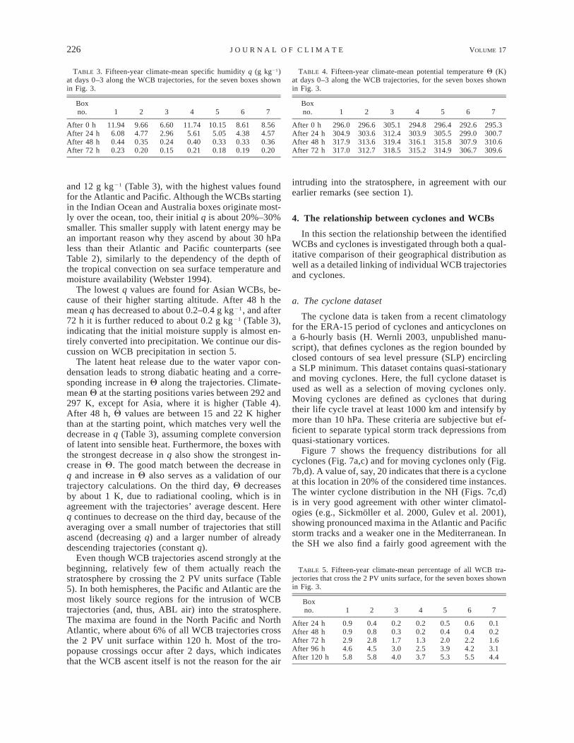
226 VOLUME 17J O U R N A L O F C L I M A T E
TABLE 3. Fifteen-year climate-mean specific humidity q (g kg21)at days 0–3 along the WCB trajectories, for the seven boxes shownin Fig. 3.
Boxno. 1 2 3 4 5 6 7
After 0 hAfter 24 hAfter 48 hAfter 72 h
11.946.080.440.23
9.664.770.350.20
6.602.960.240.15
11.745.610.400.21
10.155.050.330.18
8.614.380.330.19
8.564.570.360.20
TABLE 4. Fifteen-year climate-mean potential temperature Q (K)at days 0–3 along the WCB trajectories, for the seven boxes shownin Fig. 3.
Boxno. 1 2 3 4 5 6 7
After 0 hAfter 24 hAfter 48 hAfter 72 h
296.0304.9317.9317.0
296.6303.6313.6312.7
305.1312.4319.4318.5
294.8303.9316.1315.2
296.4305.5315.8314.9
292.6299.0307.9306.7
295.3300.7310.6309.6
TABLE 5. Fifteen-year climate-mean percentage of all WCB tra-jectories that cross the 2 PV units surface, for the seven boxes shownin Fig. 3.
Boxno. 1 2 3 4 5 6 7
After 24 hAfter 48 hAfter 72 hAfter 96 hAfter 120 h
0.90.92.94.65.8
0.40.82.84.55.8
0.20.31.73.04.0
0.20.21.32.53.7
0.50.42.03.95.3
0.60.42.24.25.5
0.10.21.63.14.4
and 12 g kg21 (Table 3), with the highest values foundfor the Atlantic and Pacific. Although the WCBs startingin the Indian Ocean and Australia boxes originate most-ly over the ocean, too, their initial q is about 20%–30%smaller. This smaller supply with latent energy may bean important reason why they ascend by about 30 hPaless than their Atlantic and Pacific counterparts (seeTable 2), similarly to the dependency of the depth ofthe tropical convection on sea surface temperature andmoisture availability (Webster 1994).
The lowest q values are found for Asian WCBs, be-cause of their higher starting altitude. After 48 h themean q has decreased to about 0.2–0.4 g kg21, and after72 h it is further reduced to about 0.2 g kg21 (Table 3),indicating that the initial moisture supply is almost en-tirely converted into precipitation. We continue our dis-cussion on WCB precipitation in section 5.
The latent heat release due to the water vapor con-densation leads to strong diabatic heating and a corre-sponding increase in Q along the trajectories. Climate-mean Q at the starting positions varies between 292 and297 K, except for Asia, where it is higher (Table 4).After 48 h, Q values are between 15 and 22 K higherthan at the starting point, which matches very well thedecrease in q (Table 3), assuming complete conversionof latent into sensible heat. Furthermore, the boxes withthe strongest decrease in q also show the strongest in-crease in Q. The good match between the decrease inq and increase in Q also serves as a validation of ourtrajectory calculations. On the third day, Q decreasesby about 1 K, due to radiational cooling, which is inagreement with the trajectories’ average descent. Hereq continues to decrease on the third day, because of theaveraging over a small number of trajectories that stillascend (decreasing q) and a larger number of alreadydescending trajectories (constant q).
Even though WCB trajectories ascend strongly at thebeginning, relatively few of them actually reach thestratosphere by crossing the 2 PV units surface (Table5). In both hemispheres, the Pacific and Atlantic are themost likely source regions for the intrusion of WCBtrajectories (and, thus, ABL air) into the stratosphere.The maxima are found in the North Pacific and NorthAtlantic, where about 6% of all WCB trajectories crossthe 2 PV unit surface within 120 h. Most of the tro-popause crossings occur after 2 days, which indicatesthat the WCB ascent itself is not the reason for the air
intruding into the stratosphere, in agreement with ourearlier remarks (see section 1).
4. The relationship between cyclones and WCBs
In this section the relationship between the identifiedWCBs and cyclones is investigated through both a qual-itative comparison of their geographical distribution aswell as a detailed linking of individual WCB trajectoriesand cyclones.
a. The cyclone dataset
The cyclone data is taken from a recent climatologyfor the ERA-15 period of cyclones and anticyclones ona 6-hourly basis (H. Wernli 2003, unpublished manu-script), that defines cyclones as the region bounded byclosed contours of sea level pressure (SLP) encirclinga SLP minimum. This dataset contains quasi-stationaryand moving cyclones. Here, the full cyclone dataset isused as well as a selection of moving cyclones only.Moving cyclones are defined as cyclones that duringtheir life cycle travel at least 1000 km and intensify bymore than 10 hPa. These criteria are subjective but ef-ficient to separate typical storm track depressions fromquasi-stationary vortices.
Figure 7 shows the frequency distributions for allcyclones (Fig. 7a,c) and for moving cyclones only (Fig.7b,d). A value of, say, 20 indicates that there is a cycloneat this location in 20% of the considered time instances.The winter cyclone distribution in the NH (Figs. 7c,d)is in very good agreement with other winter climatol-ogies (e.g., Sickmoller et al. 2000, Gulev et al. 2001),showing pronounced maxima in the Atlantic and Pacificstorm tracks and a weaker one in the Mediterranean. Inthe SH we also find a fairly good agreement with the
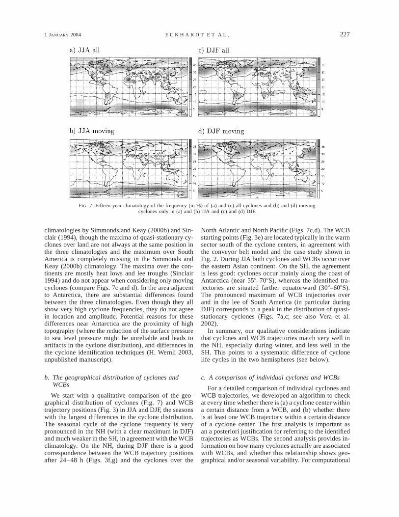
1 JANUARY 2004 227E C K H A R D T E T A L .
FIG. 7. Fifteen-year climatology of the frequency (in %) of (a) and (c) all cyclones and (b) and (d) movingcyclones only in (a) and (b) JJA and (c) and (d) DJF.
climatologies by Simmonds and Keay (2000b) and Sin-clair (1994), though the maxima of quasi-stationary cy-clones over land are not always at the same position inthe three climatologies and the maximum over SouthAmerica is completely missing in the Simmonds andKeay (2000b) climatology. The maxima over the con-tinents are mostly heat lows and lee troughs (Sinclair1994) and do not appear when considering only movingcyclones (compare Figs. 7c and d). In the area adjacentto Antarctica, there are substantial differences foundbetween the three climatologies. Even though they allshow very high cyclone frequencies, they do not agreein location and amplitude. Potential reasons for thesedifferences near Antarctica are the proximity of hightopography (where the reduction of the surface pressureto sea level pressure might be unreliable and leads toartifacts in the cyclone distribution), and differences inthe cyclone identification techniques (H. Wernli 2003,unpublished manuscript).
b. The geographical distribution of cyclones andWCBs
We start with a qualitative comparison of the geo-graphical distribution of cyclones (Fig. 7) and WCBtrajectory positions (Fig. 3) in JJA and DJF, the seasonswith the largest differences in the cyclone distribution.The seasonal cycle of the cyclone frequency is verypronounced in the NH (with a clear maximum in DJF)and much weaker in the SH, in agreement with the WCBclimatology. On the NH, during DJF there is a goodcorrespondence between the WCB trajectory positionsafter 24–48 h (Figs. 3f,g) and the cyclones over the
North Atlantic and North Pacific (Figs. 7c,d). The WCBstarting points (Fig. 3e) are located typically in the warmsector south of the cyclone centers, in agreement withthe conveyor belt model and the case study shown inFig. 2. During JJA both cyclones and WCBs occur overthe eastern Asian continent. On the SH, the agreementis less good: cyclones occur mainly along the coast ofAntarctica (near 558–708S), whereas the identified tra-jectories are situated farther equatorward (308–608S).The pronounced maximum of WCB trajectories overand in the lee of South America (in particular duringDJF) corresponds to a peak in the distribution of quasi-stationary cyclones (Figs. 7a,c; see also Vera et al.2002).
In summary, our qualitative considerations indicatethat cyclones and WCB trajectories match very well inthe NH, especially during winter, and less well in theSH. This points to a systematic difference of cyclonelife cycles in the two hemispheres (see below).
c. A comparison of individual cyclones and WCBs
For a detailed comparison of individual cyclones andWCB trajectories, we developed an algorithm to checkat every time whether there is (a) a cyclone center withina certain distance from a WCB, and (b) whether thereis at least one WCB trajectory within a certain distanceof a cyclone center. The first analysis is important asan a posteriori justification for referring to the identifiedtrajectories as WCBs. The second analysis provides in-formation on how many cyclones actually are associatedwith WCBs, and whether this relationship shows geo-graphical and/or seasonal variability. For computational
228 VOLUME 17J O U R N A L O F C L I M A T E
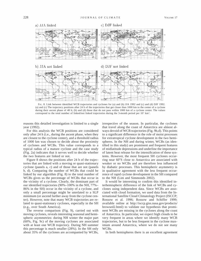
FIG. 8. Link between identified WCB trajectories and cyclones for (a) and (b) JJA 1992 and (c) and (d) DJF 1992.(a) and (c) The trajectory positions after 24 h of the trajectories that get closer than 1000 km to the center of a cycloneduring their ascent phase of 48 h; (b) and (d) those that do not pass within 1000 km of a cyclone center. The valuescorrespond to the total number of linked/not linked trajectories during the 3-month period per 10 5 km2.
reasons this detailed investigation is limited to a singleyear (1992).
For this analysis the WCB positions are consideredonly after 24 h (i.e., during the ascent phase, when theyare closest to the cyclone center), and a threshold radiusof 1000 km was chosen to decide about the proximityof cyclones and WCBs. This value corresponds to atypical radius of a mature cyclone and the case study(Fig. 2a) indicates that it serves well to decide whetherthe two features are linked or not.
Figure 8 shows the positions after 24 h of the trajec-tories that are linked with a moving or quasi-stationarycyclone (panels a, c) and of those that are not (panelsb, d). Comparing the number of WCBs that could belinked by our algorithm (Fig. 8) to the total number ofWCBs gives us the percentage of WCBs that occur inthe vicinity of a cyclone. Clearly, the dominant part ofour identified trajectories (90%–100% in the NH, 77%–86% in the SH) occur in the vicinity of a cyclone, andonly a small percentage might be unrelated to a SLPminimum (or ascend farther away from the cyclone cen-ter). However, note that many WCB trajectories are re-lated to quasi-stationary cyclones, especially in the SH(e.g., over South America).
The reverse comparison (Fig. 9), carried out withmoving cyclones, reveals interesting seasonal and hemi-spheric asymmetries: during NH winter the major part(60%, Fig. 9c) of the moving cyclones are associatedwith at least one WCB trajectory. During NH summerthis percentage is much smaller (28%). In the SH onlyabout 35% of the cyclones are accompanied by WCBs,
irrespective of the season. In particular, the cyclonesthat travel along the coast of Antarctica are almost al-ways devoid of WCB trajectories (Fig. 9b,d). This pointsto a significant difference in the role of moist processesfor extratropical cyclone development in the two hemi-spheres. In the NH and during winter, WCBs (as iden-tified in this study) are prominent and frequent featuresof midlatitude depressions and underline the importanceof latent heat release for the intensification of these sys-tems. However, the most frequent SH cyclones occur-ring near 608S close to Antarctica are associated withweaker or no WCBs and are therefore less influencedby diabatic processes. This hemispheric asymmetry isin qualitative agreement with the less frequent occur-rence of rapid cyclone development in the SH comparedto the NH (Lim and Simmonds 2002).
It would be interesting to confirm this identified in-terhemispheric difference of the link of WCBs and cy-clones using independent data. Since WCBs are asso-ciated with cloud formation, we used data from the In-ternational Satellite Cloud Climatology Project (ISCCP;Rossow et al. 1996; Rossow and Schiffer 1999;available online at http://isccp.giss.nasa.gov/products/browsed2.html) to validate our hypothesis that promi-nent WCBs are missing in the cyclones along the coastof Antarctica. In particular, we expect high clouds to bevery frequent in areas where we identify many WCBtrajectories, but to be less frequent in the cyclone max-imum around Antarctica, where we do not see manyWCBs.
In both hemispheres there is an excellent agreement
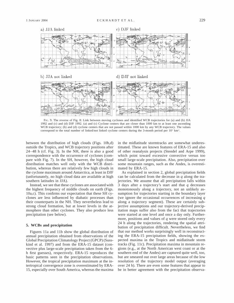
1 JANUARY 2004 229E C K H A R D T E T A L .
FIG. 9. The reverse of Fig. 8: Link between moving cyclones and identified WCB trajectories for (a) and (b) JJA1992 and (c) and (d) DJF 1992. (a) and (c) Cyclone centers that are closer than 1000 km to at least one ascendingWCB trajectory; (b) and (d) cyclone centers that are not passed within 1000 km by any WCB trajectory. The valuescorrespond to the total number of linked/not linked cyclone centers during the 3-month period per 10 5 km2.
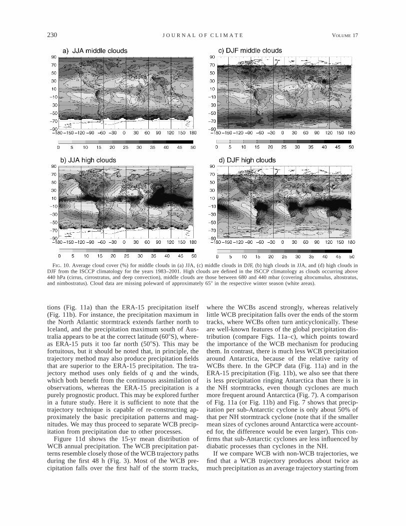
between the distribution of high clouds (Figs. 10b,d)outside the Tropics, and WCB trajectory positions after24–48 h (cf. Fig. 3). In the NH, there is also a goodcorrespondence with the occurrence of cyclones (com-pare with Fig. 7). In the SH, however, the high clouddistribution matches well only with the WCB distri-bution, whereas there are relatively few high clouds inthe cyclone maximum around Antarctica, at least in DJF(unfortunately, no high cloud data are available at highsouthern latitudes in JJA).
Instead, we see that these cyclones are associated withthe highest frequency of middle clouds on earth (Figs.10a,c). This confirms our expectation that these SH cy-clones are less influenced by diabatic processes thantheir counterparts in the NH. They nevertheless lead tostrong cloud formation, but at lower levels in the at-mosphere than other cyclones. They also produce lessprecipitation (see below).
5. WCBs and precipitation
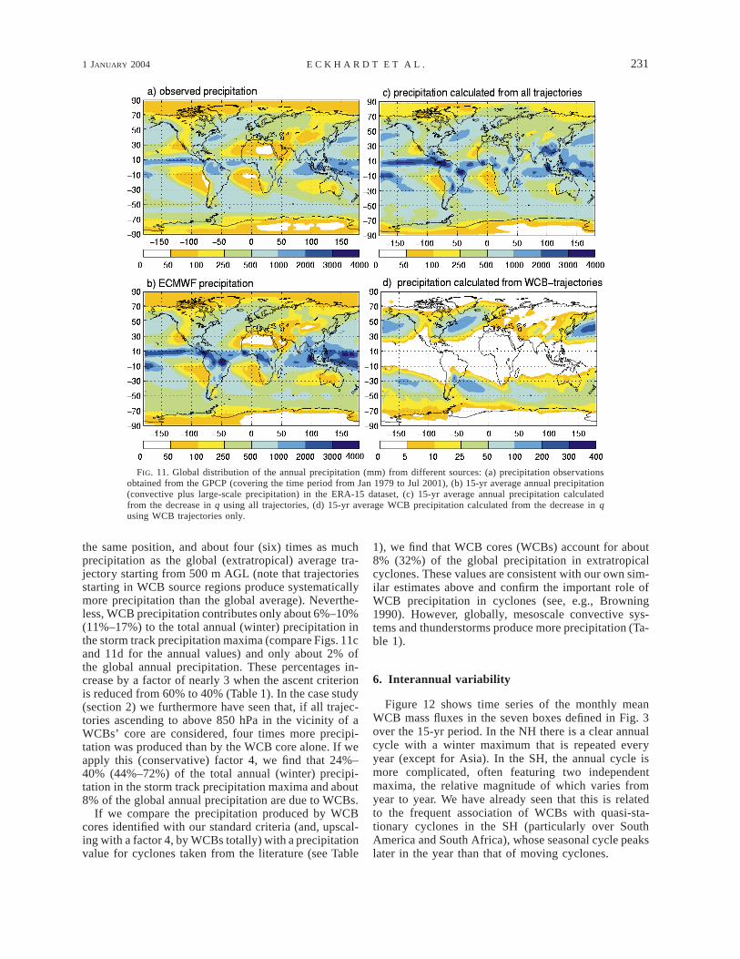
Figures 11a and 11b show the global distribution ofannual precipitation obtained from observations of theGlobal Precipitation Climatology Project (GPCP) (Suss-kind et al. 1997) and from the ERA-15 dataset (con-vective plus large-scale precipitation taken from the 6-h first guesses), respectively. ERA-15 reproduces thebasic patterns seen in the precipitation observations.However, the tropical precipitation maximum at the in-tertropical convergence zone is overestimated by ERA-15, especially over South America, whereas the maxima
in the midlatitude stormtracks are somewhat underes-timated. These are known features of ERA-15 and alsoof other reanalysis projects (Stendel and Arpe 1999),which point toward excessive convective versus toosmall large-scale precipitation. Also, precipitation oversome mountain ranges, such as the Andes, is overesti-mated by ERA-15.
As explained in section 2, global precipitation fieldscan be calculated from the decrease in q along the tra-jectories. We assume that all precipitation falls within3 days after a trajectory’s start and that q decreasesmonotonously along a trajectory, not an unlikely as-sumption for trajectories starting in the boundary layer(we ignore the occasional occurrences of increasing qalong a trajectory segment). These are certainly sub-jective assumptions and our trajectory-derived precip-itation maps suffer also from the fact that trajectorieswere started at one level and once a day only. Further-more, positions and values of q were stored only every24 h along the trajectories, rendering the spatial attri-bution of precipitation difficult. Nevertheless, we findthat our method works surprisingly well in reconstruct-ing the ERA-15 precipitation fields, showing the ex-pected maxima in the Tropics and midlatitude stormtracks (Fig. 11c). Precipitation maxima in mountain re-gions (e.g., at the North American west coast or at thesouthern end of the Andes) are captured quite well, too,but are smeared out over large areas because of the lowresolution of the trajectory model output (averagingover 24 h). There are even some features that appear tobe in better agreement with the precipitation observa-
230 VOLUME 17J O U R N A L O F C L I M A T E
FIG. 10. Average cloud cover (%) for middle clouds in (a) JJA, (c) middle clouds in DJF, (b) high clouds in JJA, and (d) high clouds inDJF from the ISCCP climatology for the years 1983–2001. High clouds are defined in the ISCCP climatology as clouds occurring above440 hPa (cirrus, cirrostratus, and deep convection), middle clouds are those between 680 and 440 mbar (covering altocumulus, altostratus,and nimbostratus). Cloud data are missing poleward of approximately 658 in the respective winter season (white areas).
tions (Fig. 11a) than the ERA-15 precipitation itself(Fig. 11b). For instance, the precipitation maximum inthe North Atlantic stormtrack extends farther north toIceland, and the precipitation maximum south of Aus-tralia appears to be at the correct latitude (608S), where-as ERA-15 puts it too far north (508S). This may befortuitous, but it should be noted that, in principle, thetrajectory method may also produce precipitation fieldsthat are superior to the ERA-15 precipitation. The tra-jectory method uses only fields of q and the winds,which both benefit from the continuous assimilation ofobservations, whereas the ERA-15 precipitation is apurely prognostic product. This may be explored furtherin a future study. Here it is sufficient to note that thetrajectory technique is capable of re-constructing ap-proximately the basic precipitation patterns and mag-nitudes. We may thus proceed to separate WCB precip-itation from precipitation due to other processes.
Figure 11d shows the 15-yr mean distribution ofWCB annual precipitation. The WCB precipitation pat-terns resemble closely those of the WCB trajectory pathsduring the first 48 h (Fig. 3). Most of the WCB pre-cipitation falls over the first half of the storm tracks,
where the WCBs ascend strongly, whereas relativelylittle WCB precipitation falls over the ends of the stormtracks, where WCBs often turn anticyclonically. Theseare well-known features of the global precipitation dis-tribution (compare Figs. 11a–c), which points towardthe importance of the WCB mechanism for producingthem. In contrast, there is much less WCB precipitationaround Antarctica, because of the relative rarity ofWCBs there. In the GPCP data (Fig. 11a) and in theERA-15 precipitation (Fig. 11b), we also see that thereis less precipitation ringing Antarctica than there is inthe NH stormtracks, even though cyclones are muchmore frequent around Antarctica (Fig. 7). A comparisonof Fig. 11a (or Fig. 11b) and Fig. 7 shows that precip-itation per sub-Antarctic cyclone is only about 50% ofthat per NH stormtrack cyclone (note that if the smallermean sizes of cyclones around Antarctica were account-ed for, the difference would be even larger). This con-firms that sub-Antarctic cyclones are less influenced bydiabatic processes than cyclones in the NH.
If we compare WCB with non-WCB trajectories, wefind that a WCB trajectory produces about twice asmuch precipitation as an average trajectory starting from
1 JANUARY 2004 231E C K H A R D T E T A L .
FIG. 11. Global distribution of the annual precipitation (mm) from different sources: (a) precipitation observationsobtained from the GPCP (covering the time period from Jan 1979 to Jul 2001), (b) 15-yr average annual precipitation(convective plus large-scale precipitation) in the ERA-15 dataset, (c) 15-yr average annual precipitation calculatedfrom the decrease in q using all trajectories, (d) 15-yr average WCB precipitation calculated from the decrease in qusing WCB trajectories only.
the same position, and about four (six) times as muchprecipitation as the global (extratropical) average tra-jectory starting from 500 m AGL (note that trajectoriesstarting in WCB source regions produce systematicallymore precipitation than the global average). Neverthe-less, WCB precipitation contributes only about 6%–10%(11%–17%) to the total annual (winter) precipitation inthe storm track precipitation maxima (compare Figs. 11cand 11d for the annual values) and only about 2% ofthe global annual precipitation. These percentages in-crease by a factor of nearly 3 when the ascent criterionis reduced from 60% to 40% (Table 1). In the case study(section 2) we furthermore have seen that, if all trajec-tories ascending to above 850 hPa in the vicinity of aWCBs’ core are considered, four times more precipi-tation was produced than by the WCB core alone. If weapply this (conservative) factor 4, we find that 24%–40% (44%–72%) of the total annual (winter) precipi-tation in the storm track precipitation maxima and about8% of the global annual precipitation are due to WCBs.
If we compare the precipitation produced by WCBcores identified with our standard criteria (and, upscal-ing with a factor 4, by WCBs totally) with a precipitationvalue for cyclones taken from the literature (see Table
1), we find that WCB cores (WCBs) account for about8% (32%) of the global precipitation in extratropicalcyclones. These values are consistent with our own sim-ilar estimates above and confirm the important role ofWCB precipitation in cyclones (see, e.g., Browning1990). However, globally, mesoscale convective sys-tems and thunderstorms produce more precipitation (Ta-ble 1).
6. Interannual variability
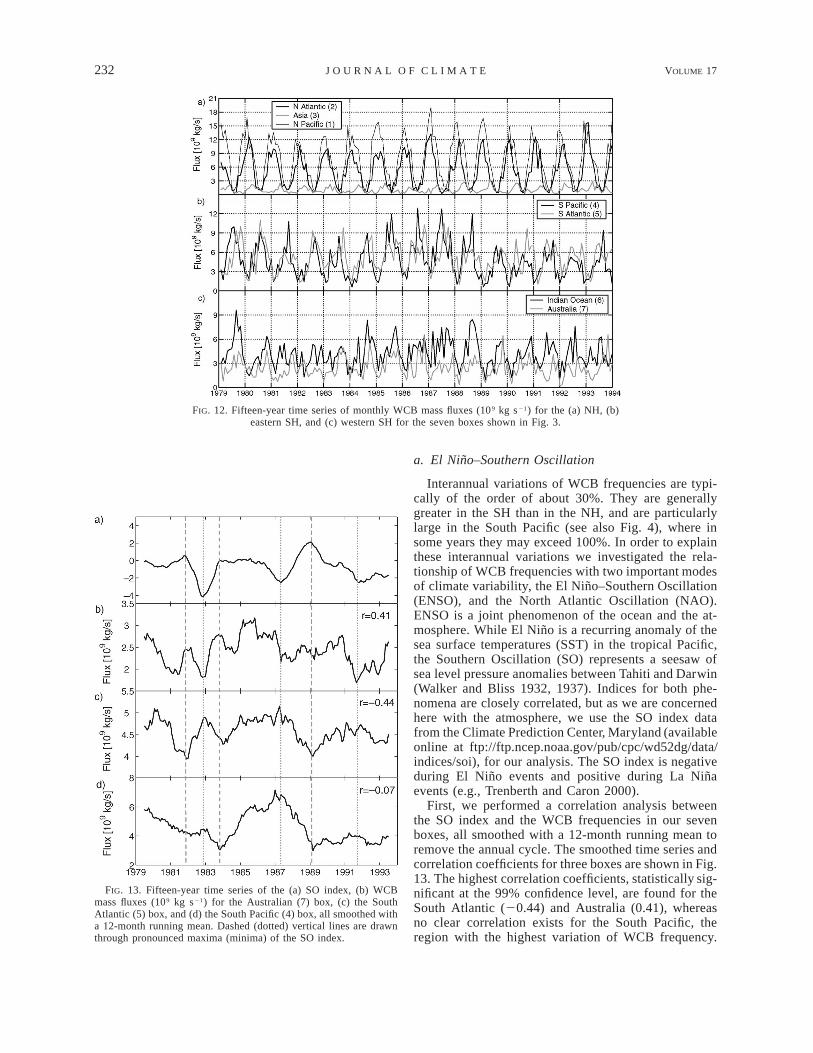
Figure 12 shows time series of the monthly meanWCB mass fluxes in the seven boxes defined in Fig. 3over the 15-yr period. In the NH there is a clear annualcycle with a winter maximum that is repeated everyyear (except for Asia). In the SH, the annual cycle ismore complicated, often featuring two independentmaxima, the relative magnitude of which varies fromyear to year. We have already seen that this is relatedto the frequent association of WCBs with quasi-sta-tionary cyclones in the SH (particularly over SouthAmerica and South Africa), whose seasonal cycle peakslater in the year than that of moving cyclones.
232 VOLUME 17J O U R N A L O F C L I M A T E
FIG. 12. Fifteen-year time series of monthly WCB mass fluxes (109 kg s21) for the (a) NH, (b)eastern SH, and (c) western SH for the seven boxes shown in Fig. 3.
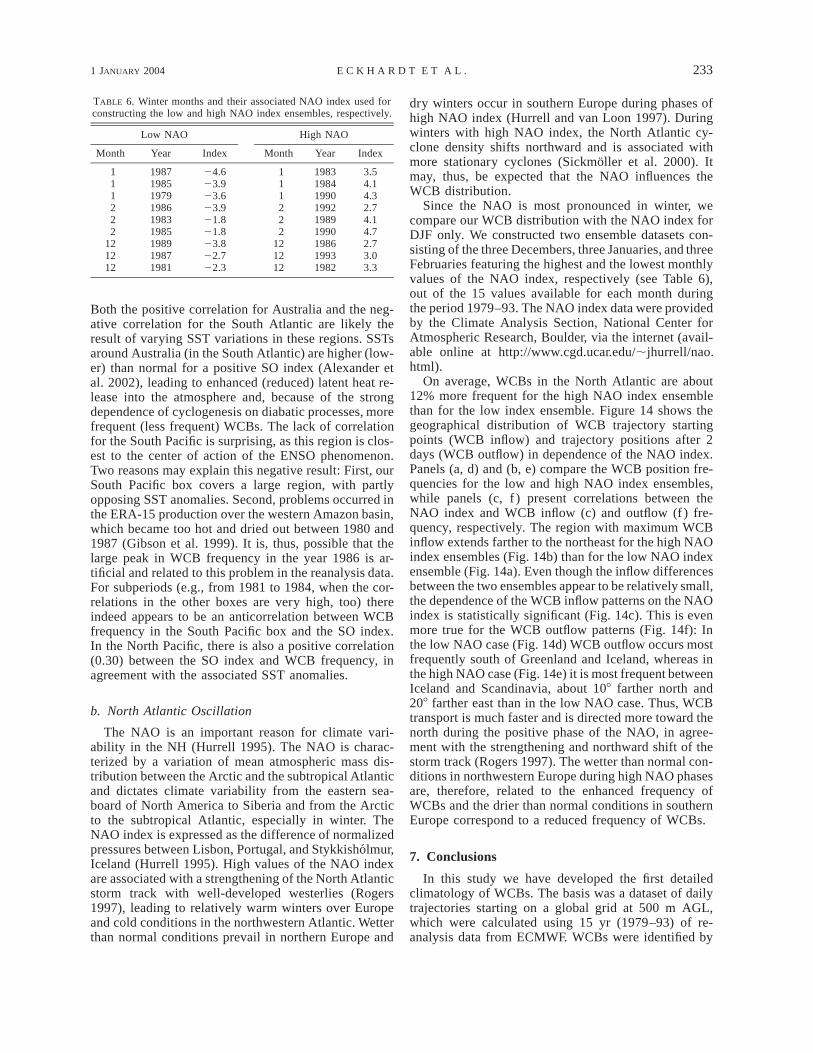
FIG. 13. Fifteen-year time series of the (a) SO index, (b) WCBmass fluxes (109 kg s21) for the Australian (7) box, (c) the SouthAtlantic (5) box, and (d) the South Pacific (4) box, all smoothed witha 12-month running mean. Dashed (dotted) vertical lines are drawnthrough pronounced maxima (minima) of the SO index.
a. El Nino–Southern Oscillation
Interannual variations of WCB frequencies are typi-cally of the order of about 30%. They are generallygreater in the SH than in the NH, and are particularlylarge in the South Pacific (see also Fig. 4), where insome years they may exceed 100%. In order to explainthese interannual variations we investigated the rela-tionship of WCB frequencies with two important modesof climate variability, the El Nino–Southern Oscillation(ENSO), and the North Atlantic Oscillation (NAO).ENSO is a joint phenomenon of the ocean and the at-mosphere. While El Nino is a recurring anomaly of thesea surface temperatures (SST) in the tropical Pacific,the Southern Oscillation (SO) represents a seesaw ofsea level pressure anomalies between Tahiti and Darwin(Walker and Bliss 1932, 1937). Indices for both phe-nomena are closely correlated, but as we are concernedhere with the atmosphere, we use the SO index datafrom the Climate Prediction Center, Maryland (availableonline at ftp://ftp.ncep.noaa.gov/pub/cpc/wd52dg/data/indices/soi), for our analysis. The SO index is negativeduring El Nino events and positive during La Ninaevents (e.g., Trenberth and Caron 2000).
First, we performed a correlation analysis betweenthe SO index and the WCB frequencies in our sevenboxes, all smoothed with a 12-month running mean toremove the annual cycle. The smoothed time series andcorrelation coefficients for three boxes are shown in Fig.13. The highest correlation coefficients, statistically sig-nificant at the 99% confidence level, are found for theSouth Atlantic (20.44) and Australia (0.41), whereasno clear correlation exists for the South Pacific, theregion with the highest variation of WCB frequency.
1 JANUARY 2004 233E C K H A R D T E T A L .
TABLE 6. Winter months and their associated NAO index used forconstructing the low and high NAO index ensembles, respectively.
Low NAO
Month Year Index
High NAO
Month Year Index
11122
19871985197919861983
24.623.923.623.921.8
11122
19831984199019921989
3.54.14.32.74.1
2121212
1985198919871981
21.823.822.722.3
2121212
1990198619931982
4.72.73.03.3
Both the positive correlation for Australia and the neg-ative correlation for the South Atlantic are likely theresult of varying SST variations in these regions. SSTsaround Australia (in the South Atlantic) are higher (low-er) than normal for a positive SO index (Alexander etal. 2002), leading to enhanced (reduced) latent heat re-lease into the atmosphere and, because of the strongdependence of cyclogenesis on diabatic processes, morefrequent (less frequent) WCBs. The lack of correlationfor the South Pacific is surprising, as this region is clos-est to the center of action of the ENSO phenomenon.Two reasons may explain this negative result: First, ourSouth Pacific box covers a large region, with partlyopposing SST anomalies. Second, problems occurred inthe ERA-15 production over the western Amazon basin,which became too hot and dried out between 1980 and1987 (Gibson et al. 1999). It is, thus, possible that thelarge peak in WCB frequency in the year 1986 is ar-tificial and related to this problem in the reanalysis data.For subperiods (e.g., from 1981 to 1984, when the cor-relations in the other boxes are very high, too) thereindeed appears to be an anticorrelation between WCBfrequency in the South Pacific box and the SO index.In the North Pacific, there is also a positive correlation(0.30) between the SO index and WCB frequency, inagreement with the associated SST anomalies.
b. North Atlantic Oscillation
The NAO is an important reason for climate vari-ability in the NH (Hurrell 1995). The NAO is charac-terized by a variation of mean atmospheric mass dis-tribution between the Arctic and the subtropical Atlanticand dictates climate variability from the eastern sea-board of North America to Siberia and from the Arcticto the subtropical Atlantic, especially in winter. TheNAO index is expressed as the difference of normalizedpressures between Lisbon, Portugal, and Stykkisholmur,Iceland (Hurrell 1995). High values of the NAO indexare associated with a strengthening of the North Atlanticstorm track with well-developed westerlies (Rogers1997), leading to relatively warm winters over Europeand cold conditions in the northwestern Atlantic. Wetterthan normal conditions prevail in northern Europe and
dry winters occur in southern Europe during phases ofhigh NAO index (Hurrell and van Loon 1997). Duringwinters with high NAO index, the North Atlantic cy-clone density shifts northward and is associated withmore stationary cyclones (Sickmoller et al. 2000). Itmay, thus, be expected that the NAO influences theWCB distribution.
Since the NAO is most pronounced in winter, wecompare our WCB distribution with the NAO index forDJF only. We constructed two ensemble datasets con-sisting of the three Decembers, three Januaries, and threeFebruaries featuring the highest and the lowest monthlyvalues of the NAO index, respectively (see Table 6),out of the 15 values available for each month duringthe period 1979–93. The NAO index data were providedby the Climate Analysis Section, National Center forAtmospheric Research, Boulder, via the internet (avail-able online at http://www.cgd.ucar.edu/;jhurrell/nao.html).
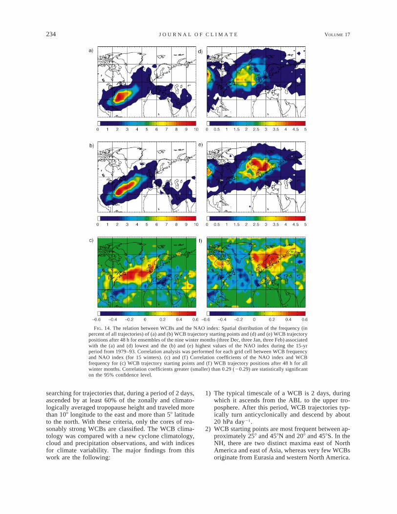
On average, WCBs in the North Atlantic are about12% more frequent for the high NAO index ensemblethan for the low index ensemble. Figure 14 shows thegeographical distribution of WCB trajectory startingpoints (WCB inflow) and trajectory positions after 2days (WCB outflow) in dependence of the NAO index.Panels (a, d) and (b, e) compare the WCB position fre-quencies for the low and high NAO index ensembles,while panels (c, f ) present correlations between theNAO index and WCB inflow (c) and outflow (f ) fre-quency, respectively. The region with maximum WCBinflow extends farther to the northeast for the high NAOindex ensembles (Fig. 14b) than for the low NAO indexensemble (Fig. 14a). Even though the inflow differencesbetween the two ensembles appear to be relatively small,the dependence of the WCB inflow patterns on the NAOindex is statistically significant (Fig. 14c). This is evenmore true for the WCB outflow patterns (Fig. 14f): Inthe low NAO case (Fig. 14d) WCB outflow occurs mostfrequently south of Greenland and Iceland, whereas inthe high NAO case (Fig. 14e) it is most frequent betweenIceland and Scandinavia, about 108 farther north and208 farther east than in the low NAO case. Thus, WCBtransport is much faster and is directed more toward thenorth during the positive phase of the NAO, in agree-ment with the strengthening and northward shift of thestorm track (Rogers 1997). The wetter than normal con-ditions in northwestern Europe during high NAO phasesare, therefore, related to the enhanced frequency ofWCBs and the drier than normal conditions in southernEurope correspond to a reduced frequency of WCBs.
7. Conclusions
In this study we have developed the first detailedclimatology of WCBs. The basis was a dataset of dailytrajectories starting on a global grid at 500 m AGL,which were calculated using 15 yr (1979–93) of re-analysis data from ECMWF. WCBs were identified by
234 VOLUME 17J O U R N A L O F C L I M A T E
FIG. 14. The relation between WCBs and the NAO index: Spatial distribution of the frequency (inpercent of all trajectories) of (a) and (b) WCB trajectory starting points and (d) and (e) WCB trajectorypositions after 48 h for ensembles of the nine winter months (three Dec, three Jan, three Feb) associatedwith the (a) and (d) lowest and the (b) and (e) highest values of the NAO index during the 15-yrperiod from 1979–93. Correlation analysis was performed for each grid cell between WCB frequencyand NAO index (for 15 winters). (c) and (f ) Correlation coefficients of the NAO index and WCBfrequency for (c) WCB trajectory starting points and (f ) WCB trajectory positions after 48 h for allwinter months. Correlation coefficients greater (smaller) than 0.29 (20.29) are statistically significanton the 95% confidence level.
searching for trajectories that, during a period of 2 days,ascended by at least 60% of the zonally and climato-logically averaged tropopause height and traveled morethan 108 longitude to the east and more than 58 latitudeto the north. With these criteria, only the cores of rea-sonably strong WCBs are classified. The WCB clima-tology was compared with a new cyclone climatology,cloud and precipitation observations, and with indicesfor climate variability. The major findings from thiswork are the following:
1) The typical timescale of a WCB is 2 days, duringwhich it ascends from the ABL to the upper tro-posphere. After this period, WCB trajectories typ-ically turn anticyclonically and descend by about20 hPa day21.
2) WCB starting points are most frequent between ap-proximately 258 and 458N and 208 and 458S. In theNH, there are two distinct maxima east of NorthAmerica and east of Asia, whereas very few WCBsoriginate from Eurasia and western North America.
1 JANUARY 2004 235E C K H A R D T E T A L .
In the SH, there is much less zonal variability, andWCB starting locations are located about 58 of lat-itude closer to the equator than in the NH.
3) WCBs occur more frequently during the winter thanduring the summer. The seasonal variation is stron-ger in the NH than in the SH. In the NH, WCBsare almost an order of magnitude more frequent inJanuary than in July.
4) WCB mass fluxes are sensitive to the WCB selec-tion criteria, but are generally 20%–60% higher inthe SH than in the NH. Our criteria identify theparticularly strong WCB cores; the total mass fluxof a WCB is about an order of magnitude higherthan that of its core. WCB mass fluxes across 850hPa are about a third of the total upward fluxes inextratropical cyclones found in other studies. WCBmass fluxes are comparable to mass fluxes in me-soscale convective systems and thunderstorms andclearly exceed those of tropical cyclones and me-soscale convective complexes.
5) The climate-mean specific humidity at WCB start-ing points in different regions varies from 7 to 12g kg21. This moisture is almost entirely convertedto precipitation, leading to an increase of potentialtemperature of 15–22 K.
6) About 6% of all WCB trajectories reach the strato-sphere within 5 days. However, the crossing of thetropopause normally occurs only after the WCB’s2 days ascent.
7) Most (90%–100% in the NH, 77%–86% in the SH)of the WCBs were found within 1000 km of a cy-clone center. The reverse comparison revealed thatmoving cyclones are normally (more than 60% ofthem) accompanied by a strong WCB only in theNH winter. In the SH, many of the WCBs are relatedto quasi-stationary cyclones at rather low latitudes(e.g., over South America). On the other hand, prac-tically no strong WCBs are found around Antarc-tica, where cyclones are globally most frequent.These cyclones are, thus, less influenced by diabaticprocesses, in agreement with their smaller growthrates. The large interhemispheric differences of therelationship between cyclones and strong WCBsalso reveal considerable differences between thegeneral circulation in the two hemispheres.
8) Outside the Tropics, there is excellent agreementbetween the distribution of WCBs and the occur-rence of high clouds obtained from a cloud cli-matology. The cyclones around Antarctica, whichare devoid of WCBs, are also less associated withhigh clouds than cyclones in other regions.
9) Using a technique to diagnose precipitation fromthe decrease of specific humidity along ascendingtrajectories, we could approximately reconstructglobal precipitation fields.
10) Over the course of 3 days, a WCB trajectory pro-duces, on average, about twice as much precipita-tion as the average trajectory starting from the same
location, and about four (six) times as much pre-cipitation as a global (extratropical) average tra-jectory starting from 500 m AGL.
11) In the winter, there is a highly significant correlationbetween the North Atlantic Oscillation and theWCB distribution in the North Atlantic: In monthswith a high NAO index, WCBs are about 12% morefrequent and their outflow occurs about 108 latitudefarther north and 208 longitude farther east than inmonths with a low NAO index. The differences inthe WCB inflow regions are relatively small be-tween the two NAO phases.
12) WCBs occur more (less) frequent around Australia(in the South Atlantic) for high phases of the South-ern Oscillation.
Acknowledgments. We thank two anonymous review-ers for their detailed comments, which helped shape thefinal version of this paper. This study was co-funded bythe German Federal Ministry for Education and Re-search within the Atmospheric Research Program 2000(AFO 2000) as part of the projects CARLOTTA andCONTRACE, and by the European Commission underContract EVK2-CT-2001-00112 (project PARTS).ECMWF and the German Weather Service are acknowl-edged for permitting access to the ECMWF archives.
REFERENCES
Alexander, M. A., I. Blade, M. Newman, J. R. Lanzante, N. C. Lau,and J. D. Scott, 2002: The atmospheric bridge: The influence ofENSO teleconnections on air–sea interaction over the globaloceans. J. Climate, 15, 2205–2231.
Arnold, F., J. Schneider, K. Gollinger, H. Schlager, P. Schulte, D. E.Hagen, P. D. Whitefield, and P. van Velthoven, 1997: Observationof upper tropospheric sulfur dioxide- and acetone-pollution: Po-tential implications for hydroxyl radical and aerosol formation.Geophys. Res. Lett., 24, 57–60.
Bethan, S., G. Vaughan, C. Gerbig, A. Volz-Thomas, H. Richer, andD. A. Tiddeman, 1998: Chemical air mass differences nearfronts. J. Geophys. Res., 103, 13 413–13 434.
Bjerknes, V., 1910: Synoptical representation of atmospheric motions.Quart. J. Roy. Meteor. Soc., 36, 167–286.
Browning, K. A., 1990: Organization of clouds and precipitation inextratropical cyclones. Extratropical Cyclones: The Erik H. Pal-men Memorial Volume, C. Newton and E. Holopainen, Eds.,Amer. Meteor. Soc., 129–153.
——, 1999: Mesoscale aspects of extratropical cyclones: An obser-vational perspective. The Life Cycles of Extratropical Cyclones,M. A. Shapiro and S. Gronas, Eds., Amer. Meteor. Soc., 265–283.
——, M. E. Hardman, T. W. Harrold, and C. W. Pardoe, 1973: Struc-ture of rainbands within a mid-latitude depression. Quart. J. Roy.Meteor. Soc., 99, 215–231.
Carlson, T. N., 1980: Airflow through midlatitude cyclones and thecomma cloud pattern. Mon. Wea. Rev., 108, 1498–1509.
——, 1998: Mid-Latitude Weather Systems. Amer. Meteor. Soc., 507pp.
Cohen, R. A., and C. W. Kreitzberg, 1997: Airstream boundaries innumerical weather simulations. Mon. Wea. Rev., 125, 168–183.
Cooper, O. R., and Coauthors, 2001: Trace gas signatures of air-streams within North Atlantic cyclones: Case studies from theNorth Atlantic Regional Experiment (NARE ’97) aircraft inten-sive. J. Geophys. Res., 106, 5437–5456.
236 VOLUME 17J O U R N A L O F C L I M A T E
——, and Coauthors, 2002: Trace gas composition of midlatitudecyclones over the western North Atlantic Ocean: A conceptualmodel. J. Geophys. Res., 4056, 107, doi:10.1029/2001JD000901.
Cotton, W. R., G. D. Alexander, R. Hertenstein, R. L. Walko, R. L.McAnelly, and M. Nicholls, 1995: Cloud venting—A reviewand some new global annual estimates. Earth Sci. Rev., 39, 169–206.
Davis, C. A., M. T. Stoelinga, and Y.-H. Kuo, 1993: The integratedeffect of condensation in numerical simulations of extratropicalcyclogenesis. Mon. Wea. Rev., 121, 2309–2330.
Gibson, J. K., P. Kallberg, S. Uppala, A. Hernandez, A. Nomura, andE. Serrano, 1999: ERA-15 Description. ECMWF re-analysisproject report series 1, version 2, ECMWF, Reading, UnitedKingdom, 77 pp.
Gulev, S. K., O. Zolina, and S. Grigoriev, 2001: Extratropical cyclonevariability in the Northern Hemisphere winter from the NCEP/NCAR reanalysis data. Climate Dyn., 17, 795–809.
Harrold, T. W., 1973: Mechanisms influencing distribution of precip-itation within baroclinic disturbances. Quart. J. Roy. Meteor.Soc., 99, 232–251.
Hoskins, B. J., and K. I. Hodges, 2002: New perspectives on theNorthern Hemisphere winter storm tracks. J. Atmos. Sci., 59,1041–1061.
——, M. E. McIntyre, and A. W. Robertson, 1985: On the use andsignificance of isentropic potential vorticity maps. Quart. J. Roy.Meteor. Soc., 111, 877–946.
Hurrell, J. W., 1995: Decadal trends in the North Atlantic Oscillation:Regional temperatures and precipitation. Science, 269, 676–679.
——, and H. Van Loon, 1997: Decadal variations in climate asso-ciated with the North Atlantic Oscillation. Climatic Change, 36,301–326.
Iskenderian, H., 1988: Three-dimensional airflow and precipitationstructure in a nondeepening cyclone. Wea. Forecasting, 3, 18–32.
Kastner, M., R. Meyer, and P. Wendling, 1999: Influence of weatherconditions on the distribution of persistent contrails. Meteor.Appl., 6, 261–271.
Kuo, Y.-H., M. A. Shapiro, and E. G. Donall, 1991: The interactionbetween baroclinic and diabatic processes in a numerical sim-ulation of a rapidly intensifying extratropical marine cyclone.Mon. Wea. Rev., 119, 368–384.
Lim, E. P., and I. Simmonds, 2002: Explosive cyclone developmentin the Southern Hemisphere and a comparison with NorthernHemisphere events. Mon. Wea. Rev., 130, 2188–2209.
Martin, J. E., 1998: The structure and evolution of a continental wintercyclone. Part II: Frontal forcing of an extreme snow event. Mon.Wea. Rev., 126, 329–348.
Massacand, A. C., H. Wernli, and H. C. Davies, 2001: Influence ofupstream diabatic heating upon an Alpine event of heavy pre-cipitation. Mon. Wea. Rev., 129, 2822–2828.
Mullen, S. L., 1987: Transient eddy forcing of blocking flows. J.Atmos. Sci., 44, 3–22.
Newell, R. E., N. E. Newell, Y. Zhu, and C. Scott, 1992: Troposphericrivers? A pilot study. Geophys. Res. Lett., 19, 2401–2404.
Peixoto, J. P., and A. H. Oort, 1992: Physics of Climate. AmericanInstitute of Physics, 520 pp.
Pomroy, H. R., and A. J. Thorpe, 2000: The evolution and dynamicalrole of reduced upper-tropospheric potential vorticity in intensiveobserving period one of FASTEX. Mon. Wea. Rev., 128, 1817–1834.
Rogers, D. C., P. J. DeMott, S. M. Kreidenweiss, and Y. Chen, 1998:Measurements of ice nucleating aerosols during SUCCESS. Geo-phys. Res. Lett., 25, 1383–1386.
Rogers, J. C., 1997: North Atlantic storm track variability and itsassociation to the North Atlantic Oscillation and climate vari-ability of northern Europe. J. Climate, 10, 1635–1647.
Rossow, W. B., and R. A. Schiffer, 1999: Advances in understandingclouds from ISCCP. Bull. Amer. Meteor. Soc., 80, 2261–2287.
——, A. W. Walker, D. E. Beuschel, and M. D. Roiter, 1996: Inter-national Satellite Cloud Climatology Project (ISCCP) documen-tation of new cloud datasets. World Climate Research Pro-gramme (ICSU and WMO) WMO/TD 737, 115 pp.
Sanders, F., and J. R. Gyakum, 1980: Synoptic-dynamic climatologyof the bomb. Mon. Wea. Rev., 108, 1589–1606.
Schultz, D. M., 2001: Reexamining the cold conveyor belt. Mon.Wea. Rev., 129, 2205–2225.
Sickmoller, M., B. Blender, and K. Fraedrich, 2000: Observed wintercyclone tracks in the Northern Hemisphere in re-analysedECMWF data. Quart. J. Roy. Meteor. Soc., 126, 591–620.
Simmonds, I., and K. Keay, 2000a: Variability of Southern Hemi-sphere extratropical cyclone behaviour, 1958–97. J. Climate, 13,550–561.
——, and ——, 2000b: Mean Southern Hemisphere extratropicalcyclone behavior in the 40-year NCEP–NCAR reanalysis. J. Cli-mate, 13, 873–885.
Sinclair, M. R., 1994: An objective cyclone climatology for the South-ern Hemisphere. Mon. Wea. Rev., 122, 2239–2256.
Stendel, M., and K. Arpe, 1999: Evaluation of the hydrological cyclein reanalyses and observations. ECMWF Re-Analysis ProjectReport Series 6, ECMWF, 53 pp.
Stewart, R. E., K. K. Szeto, R. F. Reinking, S. A. Clough, and S. P.Ballard, 1998: Midlatitude cyclonic cloud systems and their fea-tures affecting large scales and climate. Rev. Geophys., 36, 245–273.
Stoelinga, M. T., 1996: A potential vorticity-based study of the roleof diabatic heating and friction in a numerically simulated baro-clinic cyclone. Mon. Wea. Rev., 124, 849–874.
Stohl, A., 2001: A 1-year Lagrangian ‘‘climatology’’ of airstreamsin the Northern Hemisphere troposphere and lowermost strato-sphere. J. Geophys. Res., 106, 7263–7279.
——, and P. Seibert, 1998: Accuracy of trajectories as determinedfrom the conservation of meteorological tracers. Quart. J. Roy.Meteor. Soc., 124, 1465–1484.
——, and T. Trickl, 1999: A textbook example of long-range trans-port: Simultaneous observation of ozone maxima of stratosphericand North American origin in the free troposphere over Europe.J. Geophys. Res., 104, 30 445–30 462.
——, G. Wotawa, P. Seibert, and H. Kromp-Kolb, 1995: Interpolationerrors in wind fields as a function of spatial and temporal res-olution and their impact on different types of kinematic trajec-tories. J. Appl. Meteor., 34, 2149–2165.
——, L. Haimberger, M. P. Scheele, and H. Wernli, 2001: An inter-comparison of results from three trajectory models. Meteor.Appl., 8, 127–135.
——, S. Eckhardt, C. Forster, P. James, and N. Spichtinger, 2002:On the pathways and timescales of intercontinental air pollutiontransport. J. Geophys. Res., 107, 4684, doi:10.1029/2001JD001396.
——, and Coauthors, 2003: A backward modeling study of inter-continental pollution transport using aircraft measurements. J.Geophys. Res., 108, doi:10.1029/2002JD002862.
Susskind, J., P. Piraino, L. Rokke, L. Iredell, and A. Mehta, 1997:Characteristics of the TOVS pathfinder path A dataset. Bull.Amer. Meteor. Soc., 78, 1449–1472.
Trenberth, K. E., 1991: Storm tracks in the Southern Hemisphere. J.Atmos. Sci., 48, 2159–2178.
——, and J. M. Caron, 2000: The Southern Oscillation revisited: Sealevel pressures, surface temperatures and precipitation. J. Cli-mate, 13, 4358–4364.
Vera, C., P. K. Vigliarolo, and E. H. Berbery, 2002: Cold seasonsynoptic scale waves over subtropical South America. Mon. Wea.Rev., 130, 684–699.
Walker, G. T., and E. W. Bliss, 1932: World weather V. Mem. Roy.Meteor. Soc., 4, 53–84.
——, and ——, 1937: World weather VI. Mem. Roy. Meteor. Soc.,4, 119–139.

1 JANUARY 2004 237E C K H A R D T E T A L .
Wang, K.-Y., and D. E. Shallcross, 2000: A Lagrangian study of thethree-dimensional transport of boundary-layer tracers in an ide-alised baroclinic-wave life-cycle. J. Atmos. Chem., 35, 227–247.
Webster, P. J., 1994: The role of hydrological processes in ocean–atmosphere interactions. Rev. Geophys., 32, 427–476.
Wernli, H., 1997: A Lagrangian-based analysis of extratropical cy-clones, II, A detailed case study. Quart. J. Roy. Meteor. Soc.,123, 1677–1706.
——, and H. C. Davies, 1997: A Lagrangian-based analysis of ex-tratropical cyclones, I, The method and some applications.Quart. J. Roy. Meteor. Soc., 123, 467–489.
——, and M. Bourqui, 2002: A Lagrangian ‘‘1-year climatology’’ of(deep) cross-tropopause exchange in the extratropical NorthernHemisphere. J. Geophys. Res., 107, 4021, doi:10.1029/2001JD000812.
World Meteorological Organization (WMO), 1957: Meteorology—Athree dimensional science. WMO Bull., 4, 134–138.
Zhu, Y., and R. E. Newell, 1994: Atmospheric rivers and bombs.Geophys. Res. Lett., 21, 1999–2002.
Zierl, B., and V. Wirth, 1997: The influence of radiation on tropopausebehaviour and stratosphere–troposphere exchange in an uppertropospheric anticyclone. J. Geophys. Res., 102, 23 883–23 894.