N89- 22903

A 3-DIMENSIONAL FINITE-DIFFERENCE METHOD FOR CALCULATING

THE DYNAMIC COEFFICIENTS OF SEALS

F.J . Dietzen and R. Nordmann Department o f Mechanical Engineer ing

U n i v e r s i t y o f Ka ise rs lau te rn Ka ise rs lau te rn , Federal Republ ic o f Germany

This paper presents a method to calculate the dynamic coefficients of seals with arbitrary geometry. To describe the turbulent flow the Navier-Stokes equations are used in conjunction with the k-e turbulence model. These equations are solved by a full 3-dimensional finite-difference procedure instead of the normally used perturbation analysis. The time dependence of the equations is introduced by working with a coordinate system rotating with the precession frequency of the shaft. The results of this theory are compared with coefficients calculated by a perturbation analysis and with experimental results.

During the last years it has become evident that it is important to include the fluid forces caused by seals when predicting the dynamic behavior of turbopumps. To calculate these forces and the dynamic coefficients which are normally used to describe them (eq. 1)

- F;] = [-: +:] [:I + [-: 3 [:I + [-: ;] [:I several methods which are based either on the so-called "bulk-f low" theories /1 .W or directly on the Navier-Stokes equations /3.4/ have been published. A common feature of these methods, developed for straight pump seals /1/ straight gas seals 12.W or grooved seals /3/, is that they are all based on a perturbation analysis to determine the dynamic coefficients. But the perturbation analysis requires m y assumptions, e.g.

1. It so

is assumed that the shaft moves on small orbits around the centric position, that a perturbation analysis can be used for all flow variables

+ = 9, + e+, + e 2 +2.....

and all terms with power of e greater than one can be neglected in the equations without loss of accuracy (e = perturbation parameter).

21 1

https://ntrs.nasa.gov/search.jsp?R=19890013532 2020-03-10T18:49:03+00:00Z

2. The change of the perturbation flow variables in can be described by sine and cosine functions.

the circumferential direction

9, = +,, cos0 + 9 is sin0

3. The change in time can be described by

because the shaft moves on a circular orbit.

To check how these assumptions effect the results we have developed a 3-dimensional finite-difference procedure to calculate the dynamic coefficients. The only assumptions in this theory are that the turbulence can be described by the k-e turbulence model and that the shaft moves on circular orbits around the seal center.

To describe the turbulent flow in a seal we have the Navier-Stokes equations and the continuity equation. The turbulent stresses occurring in the fluid can be handled like laminar stresses by introducing a turbulent viscosity. The turbulent and the laminar viscosity are then summed up to an effective viscosity p e

To describe pt the k-e turbulence model /5.6/ is used because it is simple and

often used to calculate the turbulent flow in seals /7.8.9.10/.

All these equations can be represented in the following form

212

U

V

W

1

k

e

-

’e

’e

’e

0

’eIUk

Pee/”,

9 S

0

G - p ~ .

Table 1: Source terms of the Navier-Stokes equations, the continuity equation and the equations of the k-e model. (constants of k-e model are given in Appendix A)

To determine the dynamic coefficients we assume that the shaft moves on a circular orbit with precession frequency Q around the seal center. Since this would normally result in a time dependent problem we introduce a rotating coordinate system which is fixed at the shaft center (Fig. 1). In this system the flow is stationary. Due to the rotating coordinate system centrifugal- and Coriolis-forces occur in the equations for the radial and circumferential momentum Ill/, which are taken into consideration by a modification of the source terms.

S ’ = S V V + ~ ? r + 2 ~ w

s = sw - m 1

W

So the final form of the equations is given if Sv and Sw in Table 1 are replaced by

S’ and S i . V

213

Y

Fig. 1: Rotating coordinate system

The above given equations are solved in conjunction with the following boundary conditions (Fig. 2)

A

C

Fig. 2: Locations where the boundary-conditions must be specified

214

- uB is the average axial entrance velocity specified for every grid-plane.

For k and e the standard conditions of the k-e model /5,6/ are used at the walls.

This system of equations with the corresponding boundary conditions is solved by a 3-dimensional finite-difference procedure, based on the method published by Gosnran and Pun /E/. The seal is discretized by a grid (Fig. 3) and the variables are calculated at the nodes. To determine the pressure we use the PIS0 /13/ algorithm instead of SIMPLE /14./.

Fig. 3: Mesh arrangement in the seal

DYNAHIC OOEFFICIEMS

As result of our solution procedure we get the pressure distribution in the seal and by a pressure integration in axial and circumferential direction,the forces. To simplify the integration we consider the case when the rotating coordinate system

y, z coincides with the stationary system y. z. - -

215

L 2 R

F Y = - [ psinOridedx 0 0

When calculating the forces for 3 precession frequencies R = Ow. R = lo and R = 20 we can determine the dynamic coefficients. To save computation time we calculate k. e and p t only for R = 0 and keep it constant then for R = lo and R = 20.

1. Example

First we compare the results of the 3-dimensional theory with those of a method. based on a perturbation analysis in the Navier-Stokes equations and in addition with experimental values. For a straight seal with the following data the results are shown in Fig. 5.

L =23.5 w

r =23.5 mn i

co = 0.2 nm

W(o.e.2000 RPM)/rio = 0.13

W(o.e.4oOo RPM)/rio = 0.17

W(o.e.so00 RPM)/rio = 0.19

= 0.7*10-3 Ns/m 3 Pl p = 996.0 ks/m3 u - = 16-46 m / s

E(2000 RPM) = 0.35

t(4OOO RPM) = 0.37

f(so00 RPM) = 0.38

2. Example

For a grooved seal (Fig. 4) the dynamic coefficients are shown as a function of the groove depth €$ (Fig. 6.7).

Fig. 4: Geometry of grooved seals

216

The seal data are

L =23 .5 mn

r =23.5 mm

c = 0.2 mn i

0

= 0.7*10 -3 Ns/m 3

p = 996.0 w m 3 Vl

w(0,O.i = 14.11 m/s)/rio = 0.20

w(0.e.i = 11.76 m/s)/rio = 0.22

f(14.11 m / s ) = 0.38

f(11.76 m / s ) = 0.39

In Fig. (8.9) the grid, the axial and radial velocity,the circumferential velocity and the pressure are shown for a groove depth of 0.5 mm and an average axial velocity of i = 14.11 m/s.

3. Example

In some further calculations we have investigated the influence of grooves on the rotor and stator for the seal shown in Fig. 10.

The seal data are

3 L =35.0 mn Pl = 0.7*10-3 Ns/m

r =23.7 mn P = 996.0 kg/m3 i c = 0.2 mn n =4OOo RPM

0

f = 0.5 W(0.e) = O.*rio groove depth on rotor and stator : 0.4 mm total pressure loss : 0.8 Mpa radius of shaft orbit : r = Co/40

0

In Fig. 10 the total stiffness coefficients of the seal, and the portions developed in each part of the seal are shown.

0

217

IO00 2000 3000 4000 5000 6000 7000 - RPM [ 1 /MINI

1000 2000 3000 4000 5000 6000 7000 - RPMWMINI Fig. 5: Comparison of the dynamic coefficients for a

straight seal.

218

I

Dl d [ Ns/m 1

12 00

10 00

8 00

6 00

4 00

200

I

0 011 0,2 0,3 0,4 0,s 0,6 - H,tmml

Fig. 7: Comparison of the dynamic coefficients for grooved seals.

220

Fig. 8: Grid and axial and radial velocity for a grooved seal

221

F i g . 9: Pressure distribution and circumferential velocity for a grooved seal.

222

5,0+ 5.0 + 5J + 5.0 + 5.0 rC- 5.0 -4 35.0 1

I N h l

100 000

0

I k k

Fig. 10: Stiffness coefficients for a seal with grooves on rotor and stator

From that diagram we can draw the following interesting conclusions: 1. Although the pressure loss for a centric shaft position has the same magnitude

for every land part, these lands develop different contributions to the total coefficients.

2. Although the clearance in the chambers is 5-times greater than in the land parts, the forces in the chambers can’t be neglected.

3. The chambers have a strong destabilizing effect, because they cause positive radial forces and big positive tangential forces. (positive forces have the direction of the z-y axes in Fig. 1)

4. Example

We made further test calculations for the seal arrangement shown in Fig. 11. The seal data for this example are

-3 Ns/m 2 p1 = 0.7e

p =lo00 k%/m3 total pressure loss : 0.347 Mpa n = 2000 RPM Radius of shaft orbit : r = C 140

0 0

223

Fig. 11: Geometry of a reversing chamber

In Fig. 12 the flowfield in this seal is shown.

f

I 1.11

Fig. 12: Axial and radial velocity

I 11.11 I

19.86

X t n m

As a result the following stiffness coefficients for seal 1 and seal 2 (Fig. are obtained. 11)

seal 1 seal 2

K [N/m] - 0.128 e7 - 0.921 e5

k [N/m] - 0.133 e6 - 0.853 e5

2 24

The result is surprising. because seal 1 yields a negative direct stiffness instead of the expected positive. This can be explained if one looks at the pressure loss in the seal arrangement. I

P [ bar 4

P [burl 3

1,8 3

[ bar1 B A

P 4 e 3 1,90

f

0 U u Fig. 13: Pressure loss for Pressure loss in the Pressure loss in the

centric shaft plane with nearest plane with widest position gap in seal 1 gap in seal 1

The main pressure loss is caused by the entrance loss of the flow from the chamber into seal 2 (Fig. 1 3 ) . If now.the rotating part moves in the r-direction the increase of the clearance of seal 2 (in the plane considered) results in a sharp drop in the pressure loss B-C. And this drop in the pressure loss and the rise in the opposite plane is responsible for the negative value of k in seal 1 .

The first two examples show that the perturbation analysis yields good results in comparison with the 3-dimensional theory although it requires only a fraction of the calculation time and storage needed ior that method. On the other hand it is only possible to determine the coefficients of look-through seals with the perturbation analysis. while there are no restrictions concerning the geometry for the 3-dimensional procedure.

Example 3 and 4 clearly demonstrate that in an arrangement of several seals, the separated consideration of the single seals, even with big chambers between them, may lead to totally wrong results.

225

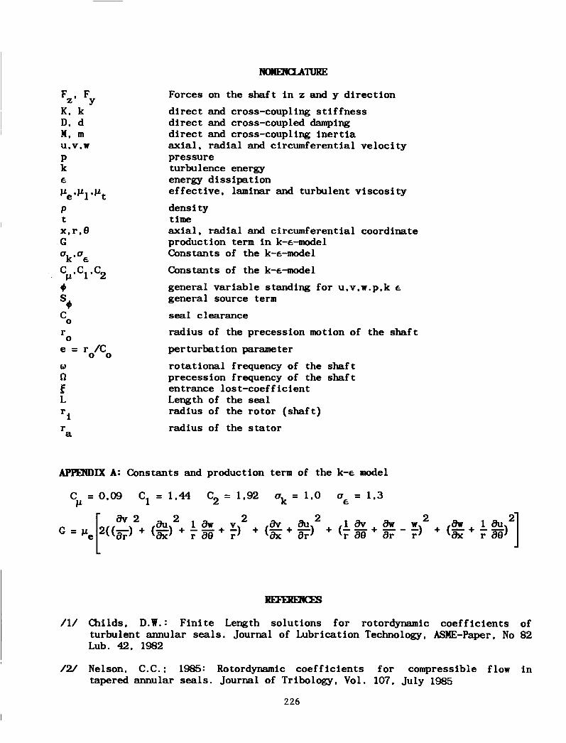
Fz* Fy K. k D. d M, m u.v.w P k e ve*vl *vt

x.r.8

P t

G k' e

c c c , p' 1' 2

9

u t 7

% cO

r 0

e = r / C 0 0

0

R f L i a

r r

Forces on the shaft in z and y direction direct and cross-coupling stiffness direct and cross-coupled damping direct and cross-coupling inertia axial, radial and circumferential velocity pressure turbulence energy energy dissipation effective, laminar and turbulent viscosity dens i ty time axial, radial and circumferential coordinate production term in k-e-model Constants of the k-e-model Constants of the k-e-mode1 general variable standing for u.v.w.p,k E. general source term seal clearance radius of the precession motion of the shaft perturbation parameter rotational frequency of the shaft precession frequency of the shaft entrance lost-coefficient Length of the seal radius of the rotor (shaft) radius of the stator

APPI.M)M A: Constants and production term of the k-e model

C = 0.09 C1 = 1.44 C2 = 1.92 uk = 1.0 u = 1,3 v e

/1/ Childs. D.W.: Finite Length solutions for rotordynamic coefficients of turbulent annular seals. Journal of Lubrication Technology, ASME-Paper, No 82 Lub. 42, 1982

/2/ Nelson, C.C.: 1985: Rotordynamic coefficients for compressible flow in tapered annular seals. Journal of Tribology. Vol. 107. July 1985

226

/3/ Dietzen. F.J.: Nordmann, R.: 1987: Calculation of rotordynamic coefficients of Seals by 'Finite-Difference' techniques. ASME Journal of Tribology, July 1987

/4/ Nordmann, R.; Dietzen. F.J.; Weiser. H.P.: Calculation of Rotordynamic Coefficients and Leakage for Annular Gas Seals by Means of Finite Difference Techniques. The 1987 ASME Design Technology Conferences - 11th Biennial Conference on Mechanical Vibration and Noise. Boston. Massachusetts, September 27-30. 1987

/5/ Launder, B.E.: Spalding. D.B.: The numerical computation of turbulent flows. Computer methods in applied mechanics and engineering. 3 (1974) 269-289

/6/ Rodi. W.: Turbulence models and their application in hydraulics. Presented by the IAHR-Section on Fundamentals of Division 11. Experimental and mathematical Fluid Dynamics

/7/ Stoff. H.: Calcule et mesure de La turbulence d'un ecoulement incompressible dans le Labyrinthe entre un arbre en rotation et un cylindre stationaire. Theses No. 342 (1949) Swiss Federal College of Technology, Lausanne. Juris Verlag Zurich, 1979

/8/ Wyssmann. H.R.: Pham. T.C.: Jenny, R.J.: Prediction of stiffness and damping coefficients for centrifugal compressor labyrinth seals. ASME Journal of Engineering for Gas Turbines and Power, Vol. 106, Oct. 1984

/9/ Rhode. D.L.; Demko. J.A.; Traegner. U.K.; Morrison, G.L.: Sobolik. S.R.: Prediction of incompressible flow in labyrinth seals. ASME Journal of Fluids Engineering, Vol. 108. March 1986

1101 Wittig. S.; Jackobsen, K.; Schelling, U.; Diirr. L.: Kim, S.: Warmeubergangszahlen in Labyrinthdichtungen. VDI-Berichte 572.1, Thermische Stromungsmaschinen '85. p. 337-356

/11/ Truckenbrodt. E., 1980: Fluidmechanik. Band 1. Grundlagen und elementare Stromungsvorgiinge dichtebesttindiger Fluide. Springer Verlag 1980. pp. 118-119

/12/ Gosnran. A.D.; Pun, W.: Lecture notes for course entitled: 'Calculation of recirculating flows'. Imperial College London. Mech. Eng. Dept.. "s /74 /2

1131 Benodekar. R.W.; Goddard. A. J.H:; Gosman. A.D.: ISSU, R.I.: Numerical prediction of turbulent flow over surfacemounted ribs. A I M Journal Vol. 23, No 3. March 1985

/14/ Patankar, S.V.: Numerical heat transfer and fluid flow. McGraw Hill Book Company ( 1 W )

1151 Mapmann. H.. 1986: Ermittlung der dynamischen Parameter turbulent durchstromter Ringspalte bei inkompressiblen Medien. Vom Fachbereich Maschinenwesen der Universitat Kaiserslautern zur Verleihung des akademischen Grades Doktor-Ingenieur genehmigte Dissertation

/16/ Diewald, W.: Nordmann. R., 1988: Influence of Different Types of Seals on the Stability Behavior of Turbopumps. The Second International Symposium on Transport Phenomena. Dynamics and Design of Rotating Machinery; Volume 2: Dynamics. Honolulu, Hawaii April 3-6, 1988.

227