Operations Research Letters 29 (2001) 41–47www.elsevier.com/locate/dsw

A 32-approximation algorithm for parallel machine scheduling

with controllable processing times

Feng Zhanga, Guochun Tanga, Zhi-Long Chenb; ∗aShanghai Second Polytechnic University, Shanghai, China

bDepartment of Systems Engineering, University of Pennsylvania, 220 South 33rd Street, Philadelphia, PA 19104-6315, USA

Received 11 September 2000; received in revised form 1 April 2001; accepted 11 May 2001

Abstract

We derive a 32 -approximation algorithm for the NP-hard parallel machine total weighted completion time problem with

controllable processing times by the technique of convex quadratic programming relaxation. c© 2001 Elsevier ScienceB.V. All rights reserved.

Keywords: Scheduling with controllable processing times; Quadratic programming; Approximation algorithm

1. Introduction

Scheduling models with job processing times being controllable through allocation of additional resourceshave received considerable attention in the last decade (see, e.g. [10,2]). These models di<er from the tra-ditional scheduling models, where job processing times are assumed to be =xed, i.e. non-controllable. Manyapplication examples of such models are described in the literature; for instances, the scheduling of toolingmachines [14] and chemical processes [11] may be characterized as scheduling models with controllable jobprocessing times.In this paper, we consider the parallel machine total weighted completion time scheduling problem with

controllable processing times. In this problem, we are given a set of n jobs J = {1; 2; : : : ; n} to be processedon a set of m unrelated parallel machines M = {1; 2; : : : ; m} such that each job only needs to be processedby one of the machines. Each job j∈ J has a weight wj ∈Z+ and a normal processing time pij ∈Z+ ∪ {0}if it is processed on machine i∈M . The processing times of jobs are controllable in the following manner.The normal processing time of job j can be reduced by up to uij units (uij ∈Z+ ∪ {0} and uij6pij) if itsprocessing on machine i is speeded up. Each unit reduction of processing time of job j on machine i requiresa cost of cij due to the fact that additional resources are necessary for the speedup. In a given schedule, let

∗ Corresponding author. Tel.: +1-215-573-4757; fax: +1-215-898-5020.E-mail address: zlchen@seas.upenn.edu (Z.-L. Chen).

0167-6377/01/$ - see front matter c© 2001 Elsevier Science B.V. All rights reserved.PII: S 0167 -6377(01)00080 -3

42 F. Zhang et al. / Operations Research Letters 29 (2001) 41–47

tij denote the reduction of processing time and Pij =pij − tij the actual processing time of job j if job j isprocessed on machine i. Let Cj denote the completion time of job j. The problem is to =nd a schedule ofthe jobs and a processing time reduction tij (tij6 uij) for each job j if it is processed on machine i suchthat the total cost including the total weighted completion time of jobs and the total cost of speedup, i.e.∑

j∈J wjCj+∑

i∈M

∑j∈J cijtij, is minimum. Following the three-=eld notation proposed by Lawler et al. [8],

we denote this problem by R|cpt|�wjCj+��cijtij, where the notation “cpt” stands for “controllable processingtimes”.The problem R|cpt|�wjCj + ��cijtij is NP-hard even when there is only one machine [6]. No results on

this problem have been reported in the literature. However, there are a handful of existing results on somespecial cases of the problem. Chen [1] gives a branch-and-bound exact solution algorithm for the problemP|cpt|�wjCj + �cjtj, where all the machines are identical, cij ≡ cj, uij = uj, and tj is the processing timereduction of job j. Cheng et al. [3] show that the problem P|cpt|�Cj +�cjtj is solvable by a polynomial-timealgorithm. Vickson [15] shows that for the problem with one machine 1|cpt|�wjCj + �cjtj, there is anoptimal schedule that satis=es the following all-or-none property: the processing time of each job j∈ J iseither fully reduced or not reduced at all, i.e. tj ∈{0; uj}, and its actual processing time Pj ∈{pj; pj − uj}.Huang and Zhang [7] give polynomial-time algorithms for the problem 1|cpt|�wjCj + �cjtj with uj ≡ u andcj ≡ c.In this paper, we propose a 3

2 -approximation algorithm for the problem R|cpt|�wjCj+��cijtij. The algorithmis based on a convex quadratic programming relaxation for an integer quadratic programming formulation ofthe problem. We are inspired by the recent successful application of convex quadratic and semide=nite pro-gramming relaxations by Skutella [12,13] to a class of parallel-machine scheduling problems where processingtimes of jobs are not controllable. Skutella gives a 3

2 -, 2-, and 2-approximation algorithm, respectively, for theproblems R‖�wjCj, R|rij|�wjCj, and R|pmtn|�wjCj. The design of these algorithms is based on the followingidea. A given problem is =rst formulated as an integer quadratic program (IQP). Then a convex quadraticprogram (CQP) is derived by relaxing the IQP. An integer solution rounded from the fractional solution ofCQP is feasible for IQP and used as an approximation solution of IQP. We extend Skutella’s analysis on theproblem R‖�wjCj to the more general problem R|cpt|�wjCj + ��cijtij.This paper is organized as follows. In Section 2 we formulate the problem R|cpt|�wjCj + ��cijtij as an

IQP, and perform some preliminary analysis. In Section 3 we form a CQP relaxation and a strengthenedrelaxation for IQP and give a 2- and 3

2 -approximation algorithm, respectively. Finally, we conclude the paperin Section 4.

2. Quadratic programming formulation

It is easy to see that there exists an optimal schedule for R|cpt|�wjCj + ��cijtij in which(i) the processing times of jobs satisfy the all-or-none property [15], i.e. the processing time reduction

tij ∈{0; uij} and the actual processing time Pij ∈{pij; pij − uij} if job j is processed on machine i∈M ; and(ii) the job sequence on each machine i∈M satis=es the WSPT rule, i.e. the jobs processed on machine i

are sequenced in the non-decreasing order of the ratio Pij=wj.Based on this observation, we can see that R|cpt|�wjCj + ��cijtij is equivalent to the following problem

with non-controllable processing times. Given a set of 2n jobs H = {1; 2; : : : ; 2n} and m unrelated parallelmachines M = {1; : : : ; m}. Each job j∈H has a weight vj and a non-controllable processing time Tij if itis processed on machine i, where vj =wj, Tij =pij − uij if j6 n, and vj =wj−n; Tij =pi;j−n if j¿n. If jobj∈H is processed on machine i, it incurs a processing cost dij with dij = cijuij if j6 n and dij =0 if j¿n.The problem is to select a subset of n jobs K ⊆ H and =nd a schedule for these jobs such that, for eachj=1; : : : ; n, exactly one of the two jobs {j; n+ j} is selected, and the sum of the total weighted completiontime and the total processing cost of these jobs is minimum.

F. Zhang et al. / Operations Research Letters 29 (2001) 41–47 43

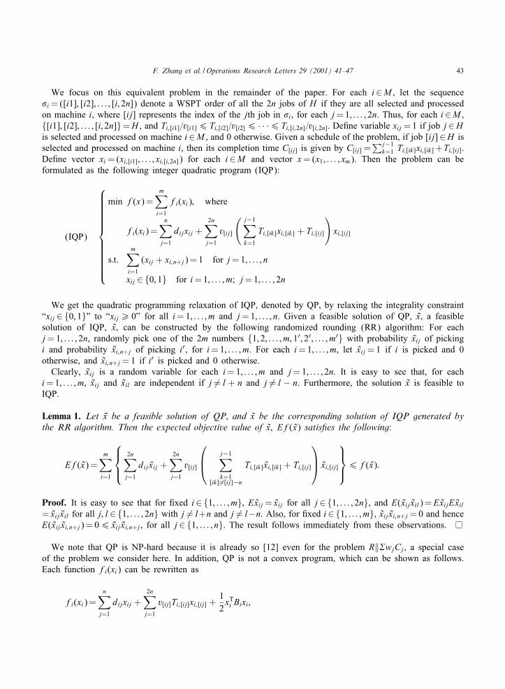
We focus on this equivalent problem in the remainder of the paper. For each i∈M , let the sequence�i =([i1]; [i2]; : : : ; [i; 2n]) denote a WSPT order of all the 2n jobs of H if they are all selected and processedon machine i, where [ij] represents the index of the jth job in �i, for each j=1; : : : ; 2n. Thus, for each i∈M ,{[i1]; [i2]; : : : ; [i; 2n]}=H , and Ti; [i1]=v[i1]6Ti; [i2]=v[i2]6 · · ·6Ti; [i;2n]=v[i;2n]: De=ne variable xij =1 if job j∈His selected and processed on machine i∈M , and 0 otherwise. Given a schedule of the problem, if job [ij]∈H isselected and processed on machine i, then its completion time C[ij] is given by C[ij] =

∑j−1k=1 Ti; [ik]xi; [ik] +Ti; [ij]:

De=ne vector xi =(xi; [i1]; : : : ; xi; [i;2n]) for each i∈M and vector x=(x1; : : : ; xm). Then the problem can beformulated as the following integer quadratic program (IQP):

(IQP)

min f(x)=m∑i=1

fi(xi); where

fi(xi)=n∑

j=1

dijxij +2n∑j=1

v[ij]

( j−1∑k=1

Ti; [ik]xi; [ik] + Ti; [ij]

)xi; [ij]

s:t:m∑i=1

(xij + xi;n+j)= 1 for j=1; : : : ; n

xij ∈{0; 1} for i=1; : : : ; m; j=1; : : : ; 2n

We get the quadratic programming relaxation of IQP, denoted by QP, by relaxing the integrality constraint“xij ∈{0; 1}” to “xij¿ 0” for all i=1; : : : ; m and j=1; : : : ; n. Given a feasible solution of QP, Nx, a feasiblesolution of IQP, x̃, can be constructed by the following randomized rounding (RR) algorithm: For eachj=1; : : : ; 2n, randomly pick one of the 2m numbers {1; 2; : : : ; m; 1′; 2′; : : : ; m′} with probability Nxij of pickingi and probability Nxi;n+j of picking i′, for i=1; : : : ; m. For each i=1; : : : ; m, let x̃ij =1 if i is picked and 0otherwise, and x̃i; n+j =1 if i′ is picked and 0 otherwise.Clearly, x̃ij is a random variable for each i=1; : : : ; m and j=1; : : : ; 2n. It is easy to see that, for each

i=1; : : : ; m, x̃ij and x̃il are independent if j �= l + n and j �= l − n. Furthermore, the solution x̃ is feasible toIQP.

Lemma 1. Let Nx be a feasible solution of QP; and x̃ be the corresponding solution of IQP generated bythe RR algorithm. Then the expected objective value of x̃; Ef(x̃) satis9es the following:

Ef(x̃)=m∑i=1

2n∑j=1

dij Nxij +2n∑j=1

v[ij]

j−1∑

k=1[ik]�=[ij]−n

Ti; [ik] Nxi; [ik] + Ti; [ij]

Nxi; [ij]

6f( Nx):

Proof. It is easy to see that for =xed i∈{1; : : : ; m}, Ex̃ij = Nxij for all j∈{1; : : : ; 2n}, and E(x̃ij x̃il)=Ex̃ijEx̃il= Nxij Nxil for all j; l∈{1; : : : ; 2n} with j �= l+n and j �= l−n. Also, for =xed i∈{1; : : : ; m}, x̃ij x̃i; n+j =0 and henceE(x̃ij x̃i; n+j)= 06 Nxij Nxi;n+j, for all j∈{1; : : : ; n}. The result follows immediately from these observations.

We note that QP is NP-hard because it is already so [12] even for the problem R‖�wjCj, a special caseof the problem we consider here. In addition, QP is not a convex program, which can be shown as follows.Each function fi(xi) can be rewritten as

fi(xi)=n∑

j=1

dijxij +2n∑j=1

v[ij]Ti; [ij]xi; [ij] +12xTi Bixi;

44 F. Zhang et al. / Operations Research Letters 29 (2001) 41–47

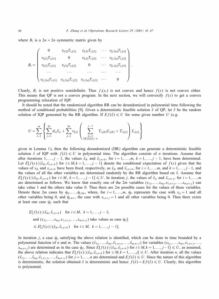
where Bi is a 2n× 2n symmetric matrix given by

Bi =

0 v[i2]Ti; [i1] v[i3]Ti; [i1] · · · v[i;2n]Ti; [i1]

v[i2]Ti; [i1] 0 v[i3]Ti; [i2] · · · v[i;2n]Ti; [i2]

v[i3]Ti; [i1] v[i3]Ti; [i2] 0 · · · v[i;2n]Ti; [i3]

· · · · · · · · · · · · · · ·v[i;2n]Ti; [i1] v[i;2n]Ti; [i2] v[i;2n]Ti; [i3] · · · 0

:

Clearly, Bi is not positive semide=nite. Thus fi(xi) is not convex and hence f(x) is not convex either.This means that QP is not a convex program. In the next section, we will convexify f(x) to get a convexprogramming relaxation of IQP.It should be noted that the randomized algorithm RR can be derandomized in polynomial time following the

method of conditional probabilities [9]. Given a deterministic feasible solution Nx of QP, let x̃ be the randomsolution of IQP generated by the RR algorithm. If Ef(x̃)6U for some given number U (e.g.

U =m∑i=1

2n∑j=1

dij Nxij +2n∑j=1

v[ij]

j−1∑

k=1[ik]�=[ij]−n

Ti; [ik] Nxi; [ik] + Ti; [ij]

Nxi; [ij]

given in Lemma 1), then the following derandomized (DR) algorithm can generate a deterministic feasiblesolution x̂ of IQP with f(x̂)6U in polynomial time. The algorithm consists of n iterations. Assume thatafter iterations 1; : : : ; j − 1, the values x̂ik and x̂i; n+k , for i=1; : : : ; m, k =1; : : : ; j − 1, have been determined.Let E[f(x) | (x̂ik ; x̂i; n+k) for i∈M; k =1; : : : ; j − 1] denote the conditional expectation of f(x) given that thevalues of xik and xi;n+k have been =xed, respectively, as x̂ik and x̂i; n+k , for i=1; : : : ; m, and k =1; : : : ; j−1, andthe values of all the other variables are determined randomly by the RR algorithm based on Nx. Assume thatE[f(x) | (x̂ik ; x̂i; n+k) for i∈M , k =1; : : : ; j− 1]6U . In iteration j, the values of x̂ij and x̂i; n+j, for i=1; : : : ; mare determined as follows. We know that exactly one of the 2m variables (x1j; : : : ; xmj; x1; n+j; : : : ; xm;n+j) cantake value 1 and the others take value 0. Thus there are 2m possible cases for the values of these variables.Denote these 2m cases by j1; : : : ; j;2m, where, for i=1; : : : ; m, ji represents the case with xij =1 and allother variables being 0, and j;m+i the case with xi;n+j =1 and all other variables being 0. Then there existsat least one case jl such that

E[f(x) | (x̂ik ; x̂i; n+k) for i∈M; k =1; : : : ; j − 1;

and (x1j; : : : ; xmj; x1; n+j; : : : ; xm;n+j) take values as case jl]

6E[f(x) | (x̂ik ; x̂i; n+k) for i∈M; k =1; : : : ; j − 1]:

In iteration j, a case jl satisfying the above relation is identi=ed, which can be done in time bounded by apolynomial function of n and m. The values (x̂1j; : : : ; x̂mj; x̂1; n+j; : : : ; x̂m;n+j) for variables (x1j; : : : ; xmj; x1; n+j; : : : ;xm;n+j) are determined as in the case jl. Since E[f(x) | (x̂ik ; x̂i; n+k) for i∈M; k =1; : : : ; j−1]6U , as assumed,the above relation indicates that E[f(x) | (x̂ik ; x̂i; n+k) for ∈M; k =1; : : : ; j]6U . After iteration n, all the values(x̂1j; : : : ; x̂mj; x̂1; n+j; : : : ; x̂m;n+j) for j=1; : : : ; n are determined and Ef(x̂)6U . Since the nature of this algorithmis deterministic, the solution obtained x̂ is deterministic and hence f(x̂)=Ef(x̂)6U . Clearly, this algorithmis polynomial.

F. Zhang et al. / Operations Research Letters 29 (2001) 41–47 45

3. Convex quadratic programming relaxation

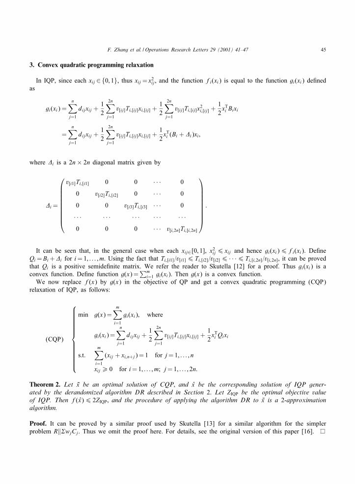
In IQP, since each xij ∈{0; 1}, thus xij = x2ij, and the function fi(xi) is equal to the function gi(xi) de=nedas

gi(xi) =n∑

j=1

dijxij +12

2n∑j=1

v[ij]Ti; [ij]xi; [ij] +12

2n∑j=1

v[ij]Ti; [ij]x2i; [ij] +12xTi Bixi

=n∑

j=1

dijxij +12

2n∑j=1

v[ij]Ti; [ij]xi; [ij] +12xTi (Bi + $i)xi;

where $i is a 2n× 2n diagonal matrix given by

$i =

v[i1]Ti; [i1] 0 0 · · · 0

0 v[i2]Ti; [i2] 0 · · · 0

0 0 v[i3]Ti; [i3] · · · 0

· · · · · · · · · · · · · · ·0 0 0 · · · v[i;2n]Ti; [i;2n]

:

It can be seen that, in the general case when each xij∈[0; 1], x2ij6 xij and hence gi(xi)6fi(xi). De=neQi =Bi +$i for i=1; : : : ; m. Using the fact that Ti; [i1]=v[i1]6Ti; [i2]=v[i2]6 · · ·6Ti; [i;2n]=v[i;2n], it can be provedthat Qi is a positive semide=nite matrix. We refer the reader to Skutella [12] for a proof. Thus gi(xi) is aconvex function. De=ne function g(x)=

∑mi=1 gi(xi). Then g(x) is a convex function.

We now replace f(x) by g(x) in the objective of QP and get a convex quadratic programming (CQP)relaxation of IQP, as follows:

(CQP)

min g(x)=m∑i=1

gi(xi); where

gi(xi)=n∑

j=1

dijxij +12

2n∑j=1

v[ij]Ti; [ij]xi; [ij] +12xTi Qixi

s:t:m∑i=1

(xij + xi;n+j)= 1 for j=1; : : : ; n

xij¿ 0 for i=1; : : : ; m; j=1; : : : ; 2n:

Theorem 2. Let Nx be an optimal solution of CQP; and x̂ be the corresponding solution of IQP gener-ated by the derandomized algorithm DR described in Section 2. Let ZIQP be the optimal objective valueof IQP. Then f(x̂)6 2ZIQP; and the procedure of applying the algorithm DR to Nx is a 2-approximationalgorithm.

Proof. It can be proved by a similar proof used by Skutella [13] for a similar algorithm for the simplerproblem R‖�wjCj. Thus we omit the proof here. For details, see the original version of this paper [16].

46 F. Zhang et al. / Operations Research Letters 29 (2001) 41–47

We can see that, in the case when each xij ∈{0; 1}, fi(xi)¿∑2n

j=1 v[ij]Ti; [ij]xi; [ij] for each i=1; : : : ; m,

and hence f(x)¿∑m

i=1

∑2nj=1 v[ij]Ti; [ij]xi; [ij]. If we add this inequality to CQP, then we get the following

strengthened relaxation of IQP.

(SP)

min z

s:t z¿m∑i=1

gi(xi)

z¿m∑i=1

2n∑j=1

v[ij]Ti; [ij]xi; [ij]

m∑i=1

(xij + xi;n+j)= 1 for j=1; : : : ; n;

xij¿ 0 for i=1; : : : ; m; j=1; : : : ; 2n:

SP is a convex program and can be solved in polynomial time within an error of ( by the ellipsoid algorithm(see, e.g. [4]). Based on SP, a better approximation algorithm can be designed as follows:Step 1: Use the ellipsoid algorithm to generate a feasible and near optimal solution of SP, ( Nx; Nz), such that

Nz¡ z∗ + 13 , where z∗ is the optimal objective value of SP.

Step 2: Apply the derandomized algorithm DR described in Section 2 to Nx and get the correspondingsolution x̂ of IQP.

Theorem 3. The solution x̂ of IQP generated by the above algorithm satis9es: f(x̂)6 32ZIQP; where ZIQP

denotes the optimal objective value of IQP; and the above algorithm is a 32 -approximation algorithm.

Proof. Clearly, for each i=1; : : : ; m,

fi( Nxi)= gi( Nxi) +12

2n∑

j=1

v[ij]Ti; [ij] Nxi; [ij] − NxTi $i Nxi

6 gi( Nxi) +

12

2n∑j=1

v[ij]Ti; [ij] Nxi; [ij]:

Thus,

f( Nx)=m∑i=1

fi( Nxi)6m∑i=1

gi( Nxi) +12

m∑i=1

2n∑j=1

v[ij]Ti; [ij] Nxi; [ij]6 g( Nx) +12

m∑i=1

2n∑j=1

v[ij]Ti; [ij] Nxi; [ij]:

Since ( Nx; Nz) is a feasible solution of SP, we have Nz¿∑m

i=1 gi( Nxi) and Nz¿∑m

i=1

∑2nj=1 v[ij]Ti; [ij] Nxi; [ij]. Then we

can get f( Nx)6 32 Nz. Since Nz¡ z∗ + 1

3 , we have f( Nx)¡ 32 z

∗ + 12 :

Clearly, the solution Nx is feasible to QP. Let x̃ be the corresponding solution of IQP generated by ap-plying the randomized RR algorithm described in Section 2 to Nx. By Lemma 1, Ef(x̃)6f( Nx). Therefore,Ef(x̃)¡ 3

2 z∗+ 1

2 . Thus, by the nature of the algorithm DR, f(x̂)¡ 32 z

∗+ 12 . Since all the parameters involved

in the function f and SP are integers, it must be true that f(x̂)6 32 z

∗. It is easy to see that the abovealgorithm is polynomial. This proves the theorem.

4. Conclusion

We have designed a 2- and 32 -approximation algorithm, respectively, for the problem R|cpt|�wjCj+��cijtij.

The design and analysis of these algorithms are based on convex programming relaxations of the problem.The results we derived here extend those obtained by Skutella [12,13] for similar scheduling problems butwith non-controllable processing times. We note that, by the work of Hoogeveen et al. [5], there does not exist

F. Zhang et al. / Operations Research Letters 29 (2001) 41–47 47

a PTAS for the problem studied here unless P=NP. Interesting topics for future research include developingtighter approximation algorithms for the same problem, and designing similar algorithms for other schedulingproblems with controllable processing times.

Acknowledgements

The =rst two authors are supported in part by the National Natural Science Foundation of China (Grant No.19771057), and the third author is supported in part by the University of Pennsylvania Research Foundationand the National Science Foundation under grant DMI-9988427.

References

[1] Z.-L. Chen, Simultaneous job scheduling and resource allocation on parallel machines. Working Paper, Department of SystemsEngineering, University of Pennsylvania, Philadelphia, PA, 1999.

[2] Z.-L. Chen, Q. Lu, G. Tang, Single machine scheduling with discretely controllable processing times, Oper. Res. Lett. 21 (1997)69–76.

[3] T.C.E. Cheng, Z.-L. Chen, C.-L. Li, Parallel machine scheduling with controllable processing times, IIE Trans. 28 (1996) 177–180.[4] M. GrRotschel, L. LovSasz, A. Schrijver, Geometric Algorithms and Combinatorial Optimization, 2nd Corrected Edition, Springer,

Berlin, Heidelberg, 1998.[5] J.A. Hoogeveen, P. Schuurman, G. Woeginger, Non-approximability results for scheduling problems with minsum criteria,

Proceedings of IPCO 98, pp. 353–366.[6] J.A. Hoogeveen, G.J. Woeginger, Scheduling with controllable processing times. Manuscript, Department of Mathematics, TU Graz,

Graz, Austria, 1998.[7] W. Huang, F. Zhang, An O(n2) algorithm for a controllable machine scheduling problem, IMA J. Math. Appl. Business Industry

10 (1999) 15–26.[8] E.L. Lawler, J.K. Lenstra, A.H.G. Rinnooy Kan, D.B. Shmoys, Sequencing and scheduling: Algorithms and complexity, in:

S. Graves, A.H.G. Rinnooy Kan, P. Zipkin (Eds.), Handbooks in Operations Research and Management Science, Vol. 4, Logisticsof Production and Inventory, North-Holland, Amsterdam, 1993, pp. 445–522.

[9] R. Motwani, P. Raghavan, Randomized Algorithms, Cambridge University Press, Cambridge, 1995.[10] E. Nowicki, S. Zdrzalka, A survey of results for sequencing problems with controllable processing times, Discrete Appl. Math. 26

(1990) 271–287.[11] E. Nowicki, S. Zdrzalka, A bicriterion approach to preemptive scheduling of parallel machines with controllable job processing

times, Discrete Appl. Math. 63 (1995) 237–256.[12] M. Skutella, Semide=nite relaxation for parallel machine scheduling, Proceedings of 39th Annual IEEE Symposium on Foundations

of Computer Science, 1998, pp. 472–481.[13] M. Skutella, Convex quadratic and semide=nite programming relaxations in scheduling, J. Assoc. Comput. Mach. 48 (2001) 206–242.[14] M. Trick, Scheduling multiple variable-speed machines, Oper. Res. 42 (1994) 234–248.[15] R.G. Vickson, Choosing the job sequence and processing times to minimize total processing plus Vow cost on single machine, Oper.

Res. 28 (1980) 1155–1167.[16] F. Zhang, G. Tang, Z.-L. Chen, A 3

2 -approximation algorithm for parallel machine scheduling with controllable processing times,Working paper, Department of Systems Engineering, University of Pennsylvania, Philadelphia, PA, 2000.